Universal fluctuations of global geometrical measurements in planar clusters

Abstract

We characterize universal features of the sample-to-sample fluctuations of global geometrical observables, such as the area, width, length, and center-of-mass position, in random growing planar clusters. Our examples are taken from simulations of both continuous and discrete models of kinetically rough interfaces, including several universality classes, such as Kardar-Parisi-Zhang. We mostly focus on the scaling behavior with time of the sample-to-sample deviation for those global magnitudes, but we have also characterized their histograms and correlations.

I Introduction

Characterizing the statistical properties of rough interfaces away from equilibrium is one of the main tasks in a variety of scientific contexts, such as the growth of solid phases in contact with a vapour Barabasi , liquid-crystal turbulence Takeuchi.11 , the shapes of isochrone curves on rough terrains Santalla.15 ; Cordoba.18 , the growth of bacterial colonies or cell aggregates Santalla.18 , or even the shape of a city skyline Najem.20 . One of the most relevant insights was provided by the Family-Vicsek (FV) dynamic scaling Ansatz Family.85 , which proposed that the width, or roughness, of a rough interface grows with time $t$ as a power-law, $W\sim t^{\beta}$, where $\beta$ is called the growth exponent, up to a saturation $t_{\text{sat}}\sim L^{z}$, where $z$ is called the dynamical exponent and $L$ is the lateral size of the system. The FV Ansatz suggests the existence of a well-defined correlation length, $\xi\sim t^{1/z}$, such that the roughness at length-scales $\ell\ll\xi$ will always be saturated, $w(\ell)\sim\ell^{\alpha}$, where $\alpha$ is the roughness exponent, the three exponents being related as $\alpha=\beta z$ within the FV formalism Barabasi ; Halpin.15 .

The values of the scaling exponents $\beta$ and $z$ are typical hallmarks of the kinetic roughening universality class. For example, for one-dimensional (1D) interfaces, $\beta=1/3$ and $z=3/2$ in the Kardar-Parisi-Zhang (KPZ) universality class Kardar.86 ; Barabasi ; Halpin.15 , which is associated with growth along the local normal direction combined with surface tension effects and time-dependent noise. Interestingly, the KPZ universality class is able to fix also the one-point and the two-point (correlation) statistics of the local interface or front fluctuations, which are associated with Airy processes of different types, depending on whether the overall symmetry of the growth system is e.g. flat or circular Praehofer.02 ; Takeuchi.11 ; Corwin.13 ; Halpin.15 . Additionally, the statistical properties of global system quantities like the (squared) roughness $W^{2}$ has been characterized in detail for globally flat KPZ interfaces (the case for e.g. periodic boundary conditions) Foltin.94 ; Antal.02 ; Halpin.15 . Notably, an equivalent result seems to be lacking for the case of growing two-dimensional clusters, which in general remains somewhat less understood, in spite of its large interest for diverse contexts from epitaxial growth Misbah.10 to cellular aggregates Muzzio.16 . For instance, as clarified in Ref. Ferreira.06 , the additional degrees of freedom implied by the dynamics of 2D clusters (like the evolution of their center of mass) has sometimes even led to incorrect identification of exponent values and universality classes for their corresponding 1D fronts. More recently Saito.12 , suitable characterizations of the cluster dynamics has been shown to extract correct exponent values and even the detailed time evolution for certain measures of 2D clusters under growth or dissolution conditions.

The aim of the present article is to characterize global properties defined in each case as a whole for 2D growing clusters. Through a scaling analysis, non-trivial predictions, like scaling exponent values, will be derived from general considerations on the sample-to-sample fluctuations of such properties. Specifically, we will consider the average radius $R$, the total area $A$, the total width $W$, the (suitably regularized) length $L$, and the center-of-mass displacement, $R_{\text{cm}}$. As we will show, the expected values of these magnitudes and their deviations grow as power laws of time, with exponents which depend on the values of $\beta$ and $z$. Previous attempts to predict the sample-to-sample fluctuations of global variables have been made in the past. For example, the center-of-mass displacement was predicted to grow as $t^{1/6}$ in KPZ clusters Saito.12 , as we here confirm for some additional examples. Moreover, we will also describe the correlation between these global magnitudes and their full histograms, which in some cases is Gaussian, and for $R_{\text{cm}}^{2}$ we will show that it corresponds to a $\chi^{2}$-distribution. The case of the squared global roughness $W^{2}$, which has been extensively studied for globally flat interfaces Foltin.94 ; Antal.02 ; Halpin.15 , is more involved, but seems to share some similarities with its flat counterpart.

We will apply our scaling estimates to simulations of growing planar clusters generated by different physical systems, whose interfaces (boundaries) are known to follow FV scaling. We will start by discussing neighborhoods (balls) in the first-passage percolation (FPP) model, whose boundaries present 1D KPZ universality in the asymptotic regime Hammersley.65 ; Cordoba.18 if discrete lattice effects are suitably taken into account Alvarez.23 . Typical FPP balls are shown in Fig. 1 (a) and (b), depending on the level of disorder. The continuous analogue of FPP is called the random metric problem, where we consider isochrone curves on a two-dimensional manifold with a random (disordered) metric field which is flat on average, with only short-range correlations Santalla.15 . Typical isochrones are shown in Fig. 1 (c). Interestingly, different types of one-point and two-point correlation functions are obtained depending on whether the underlying manifold is a plane, a cone or a cylinder Santalla.17 , although all these cases belong to the 1D KPZ universality class.

Additional interesting examples of rough interfaces with overall circular geometry are provided by the fronts of growing bacterial colonies BenJacob.00 , for which the most relevant physical parameters are the motility and the nutrient concentration. For many values of these parameters 1D KPZ scaling can be observed, but other behaviors are also possible. Specifically, for low motility and low nutrient concentration, shadowing effects —whereby the growth rate at each interface point depends on the angle under which the exterior of the cluster can be seen Santalla.18 — dominate the interfacial dynamics. In Fig. 1 (d) we show a typical time evolution for an interface described by this shadowing model.

This article is organized as follows. In Sec. II we discuss our theoretical framework in order to determine the scaling exponents for global magnitudes of clusters following FV scaling. Our predictions are then tested on FPP clusters, random metrics isochrones, and bacterial colonies in Sec. III. Additional results for the histograms and the correlations between magnitudes, are reported in Sec. IV. The article ends with a summary of our conclusions and some proposals for further work.

           

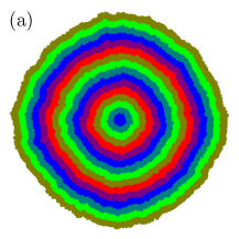
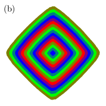
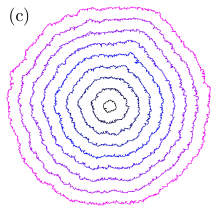
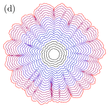
Figure 1: Typical profiles for the different physical examples considered in this article (see definitions in Sec. III). In all cases, different colors represent different growth times. (a) FPP ball with $d_{c}=1$; (b) FPP ball with $d_{c}=20$; (c) isochrone curves in the random metrics problem; (d) consecutive snapshots of the time evolution of the interface in the shadowing model of bacterial colony growth.

II Fluctuations of global geometrical observables

Let us consider a growing planar cluster whose boundary is described by a polar curve advancing in time, $r(\theta,t)$, subject to a stochastic evolution law which we may assume (along with the initial condition) to be isotropic. Let us also consider a local observable $u$ which is a function of $r$, of $r^{\prime}\equiv dr/d\theta$, and of $\theta$ itself, which we will denote by $u(r(\theta),r^{\prime}(\theta),\theta)$ or just $u(\theta)$ for short when it is convenient. Its two-point correlation function can be defined as

$$C_{u}(\hat{\theta})\equiv\left\langle u(\theta)u(\theta+\hat{\theta})\right\rangle-\left\langle u(\theta)\right\rangle\left\langle u(\theta+\hat{\theta})\right\rangle,$$ (1)

where we will denote the angular distance between the two points by $\hat{\theta}$. In the asymptotic regime, we assume the following scaling form for the correlation function,

$$C_{u}(\hat{\theta})\approx A_{u}t^{2\phi_{u}}g_{2}(B_{u}t^{1-\zeta}\hat{\theta}),$$ (2)

where $\phi_{u}$ is the corresponding scaling exponent, $A_{u}$ and $B_{u}$ are constants, $\zeta=1/z$ is the inverse of the dynamical exponent, and $g_{2}(x)$ is a continuous function such that $g(x)\sim 1$ for $x\ll 1$, and $g(x)\to 0$ sufficiently fast for $x\to\infty$.

The reason behind the form of Eq. (2) is as follows. Assuming that the expected value of the radius grows as $\left\langle r\right\rangle\sim t$ and that the correlation length grows as $\xi\sim t^{\zeta}$, as it is the case in the Family-Vicsek Ansatz Family.85 , then the angular aperture of each correlated patch along the front will be $\delta\theta_{0}\sim t^{\zeta-1}$. Then, the argument of the $g_{2}(x)$ function should be $\delta\theta/\delta\theta_{0}$, as shown in Eq. (2).

As a first example, let us consider a cluster family corresponding to the KPZ universality class Kardar.86 and the local observable $u=r$. In that case, we have $\phi_{u}=\beta=1/3$, and $C_{r}(\hat{\theta})\sim t^{2\beta}g_{2}(B_{r}t^{1-\zeta}\hat{\theta})$, where $\zeta=1/z=2/3$. Assuming that our cluster ensemble possesses a well-defined correlation length, it seems appropriate to assume that all scaling observables will present a similar structure in their correlation functions.

Let us now consider the statistical distribution of the values of a global measure of geometric origin, such as the area or the length, which can be written as

$$U=\int_{0}^{2\pi}d\theta\;u(r,r^{\prime},\theta),$$ (3)

This work is devoted to evaluating the sample-to-sample fluctuations of any global measure $U$, which will be quantified through their deviation, $\Delta U$, or their variance,

$$\textrm{Var}(U)\equiv(\Delta U)^{2}\equiv\left\langle U^{2}\right\rangle-\left\langle U\right\rangle^{2}.$$ (4)

The first two moments can be written as

$$\left\langle U\right\rangle =\int_{0}^{2\pi}d\theta\;\left\langle u(\theta)\right\rangle,$$

$$\left\langle U^{2}\right\rangle =\int_{0}^{2\pi}d\theta\int_{0}^{2\pi}d\theta^{\prime}\;\left\langle u(\theta)u(\theta^{\prime})\right\rangle,$$ (5)

thus allowing us to use a more compact notation for the variance of $U$,

$$\textrm{Var}(U) =\int d\theta d\theta^{\prime}\;\left\langle u(\theta)u(\theta^{\prime})\right\rangle-\left\langle u(\theta)\right\rangle\left\langle u(\theta^{\prime})\right\rangle$$

$$=\int d\theta d\theta^{\prime}\;C_{u}(\theta-\theta^{\prime}),$$ (6)

where $C_{u}(\theta-\theta^{\prime})$ is again the correlation function for the observable $u$, defined in Eq. (1). Thus, we can compute the variance of $U$:

$$\textrm{Var}(U) =\int d\theta d\theta^{\prime}\;C_{u}(\hat{\theta})=2\pi\int_{0}^{2\pi}d\hat{\theta}\;C_{u}(\hat{\theta})$$

$$=2\pi A_{u}t^{2\phi_{u}}\int_{0}^{2\pi}d\hat{\theta}\;g_{2}(B_{u}t^{1-\zeta}\hat{\theta})$$

$$\approx{2\pi A_{u}\over B_{u}}t^{2\phi_{u}+\zeta-1}\int_{0}^{\infty}dx\;g_{2}(x).$$ (7)

Assuming that $g_{2}(x)$ decays fast enough for large values of its argument, the last integral is finite and does not affect the scaling behavior, thus leading to an estimate for the sample-to-sample deviation of $U$,

$$\Delta U\sim t^{\phi_{u}+(\zeta-1)/2}.$$ (8)

This expression can be motivated in a heuristic way as follows. The variance of the average of $N$ independent identically distributed (i.i.d.) random variables $\left\{u_{i}\right\}$ is $\textrm{Var}(\bar{u})=\textrm{Var}(u)/N$. Yet, if these random variables are strongly correlated among themselves, with $N_{P}$ independent groups, then it is straightforward to prove that $\textrm{Var}(\bar{u})=\textrm{Var}(u)/N_{P}$. If the system radius grows approximately as $t$ and the correlation length grows as $t^{\zeta}$, then each profile possesses $n_{P}\sim t^{1-\zeta}$ independent patches. Therefore, the variance of a global variable $U$ must be given by

$$\Delta U\sim{\Delta u\over\sqrt{n_{P}}}\sim t^{\phi_{u}+(\zeta-1)/2},$$ (9)

which coincides with the result shown in Eq. (8).

The rest of this section is devoted to the theoretical analysis of the sample-to-sample fluctuations of several global geometrical observables, such as the (average) radius, area, width, center of mass position, and interfacial length.

II.1 Radius

As it has been discussed above, the sample-to-sample fluctuations of the average radius of the cluster,

$$R=\int_{0}^{2\pi}d\theta\;{r\over 2\pi},$$ (10)

can be obtained by applying our formalism to the observable $u(r,r^{\prime},\theta)=r$, which has the associated scaling exponent $\phi_{r}=\beta$, thus yielding the prediction $\Delta R\sim t^{\beta+(\zeta-1)/2}$. For example, in the 1D KPZ case, $\Delta R\sim t^{1/6}$, which has been numerically verified for balls in random metrics Santalla.15 .

II.2 Area

Let us now consider the cluster area, which is given by

$$A=\int_{0}^{2\pi}d\theta\;{r^{2}\over 2}.$$ (11)

Within our formalism, its sample-to-sample fluctuations can be obtained choosing $u(r,r^{\prime},\theta)=r^{2}$. The associated scaling exponent can be found through classical uncertainty propagation, $\Delta(r^{2})\sim r\Delta r\sim t^{1+\beta}$. Thus, $\Delta A\sim t^{\beta+(\zeta+1)/2}$. For 1D KPZ, our prediction is $\Delta A\sim t^{7/6}$.

II.3 Width

In our next example we will consider the sample-to-sample fluctuations of the interface width, defined as

$$W^{2}=\int_{0}^{2\pi}d\theta\;\frac{(r-R)^{2}}{2\pi},$$ (12)

so that the fluctuations in $W^{2}$ can be obtained using our rule. The integrand $(r-R)^{2}$ has fluctuations of order $t^{2\beta}$. Thus, its variance scales as $t^{4\beta}$, and we have

$$\textrm{Var}(W^{2})\sim t^{4\beta-1+\zeta},$$ (13)

which yields $\Delta(W^{2})\sim t^{2\beta-1/2+\zeta/2}$. Yet, we have $\Delta(W^{2})\sim W\Delta W$ and $W\sim t^{\beta}$, leading us to predict

$$\Delta W\sim t^{\beta-1/2+\zeta/2}.$$ (14)

For example, in 1D KPZ, we have $\Delta W\sim t^{1/6}$.

II.4 Center-of-mass position

In absence of fluctuations, the center-of-mass (CM) of a growing cluster starting out as a tiny circle must remain at the origin. But, even though the statistical properties of the cluster are isotropic, each sample presents unbalances which will give rise to fluctuations in the CM position Ferreira.06 ; Saito.12 ,

$$X_{\text{cm}} ={1\over A}\int_{0}^{2\pi}d\theta\;{r^{3}\over 2}\cos(\theta),$$

$$Y_{\text{cm}} ={1\over A}\int_{0}^{2\pi}d\theta\;{r^{3}\over 2}\sin(\theta).$$ (15)

Each of them presents an expectation value of zero, and a non-zero variance, which shows up in the expected value of the squared displacement,

$$R_{\text{cm}}^{2}=X_{\text{cm}}^{2}+Y_{\text{cm}}^{2}\geq 0.$$ (16)

Let us evaluate the sample-to-sample fluctuations of the following associated magnitude, which neglects the explicit angular dependence,

$$U=\int_{0}^{2\pi}d\theta\;{r^{3}\over 2},$$ (17)

and analyzing the local fluctuations of $u(r,r^{\prime},\theta)=r^{3}/2$, i.e. $\Delta u\sim t^{2+\beta}$. Thus, we have $\textrm{Var}(U)\sim t^{4+2\beta+\zeta-1}$. Now, we may guess that the scaling behavior of $U$ is the same as that for $X_{\text{cm}}A$ or $Y_{\text{cm}}A$. Thus, employing the usual uncertainty propagation techniques,

$$\Delta X_{\text{cm}}\approx{\Delta U\over A}+U{\Delta A\over A^{2}}.$$ (18)

Both terms scale in the same way, as $t^{\beta+(1-\zeta)/2}$. Thus,

$$R_{\text{cm}}^{2}\sim t^{2\beta+\zeta-1}.$$ (19)

Thus, the center of mass fluctuates with the same exponent as the average radius. For 1D KPZ, this leads to $R_{\text{cm}}\sim t^{1/6}$ Saito.12 .

II.5 Length

The length of a cluster, $L$, is a different type of observable. First of all, its measure may depend on the UV-cutoff if the interface presents a non-trivial fractal nature. Yet, we will assume that the interface is always smooth at the microscopic level and that the total length increases linearly in time, $L\sim t$. If the (radial) slopes are small, i.e. $r^{\prime}/r\ll 1$, we may write,

$$L =\int_{0}^{2\pi}d\theta\;\sqrt{r^{2}+r^{\prime 2}}=\int_{0}^{2\pi}d\theta\;r\sqrt{1+\left({r^{\prime}\over r}\right)^{2}}$$

$$\approx\int_{0}^{2\pi}d\theta\;\left(r+{1\over 2}{r^{\prime 2}\over r}\right),$$ (20)

which forces us to consider the fluctuations of the local derivative of the radius with respect to the angle, $r^{\prime}(\theta)$. In order to do that, let us consider a small angle difference, $\delta\theta$, and evaluate

$$r^{\prime}\approx{r(\theta+\delta\theta)-r(\theta)\over\delta\theta},$$ (21)

so we have

$$\textrm{Var}(r^{\prime})= \left\langle r^{\prime 2}\right\rangle-\left\langle r^{\prime}\right\rangle^{2}={2\over\delta\theta^{2}}\left[\textrm{Var}(r)-C_{r}(\delta\theta)\right]$$

$$= {2t^{2\beta}\over\delta\theta^{2}}\left[g_{2}(0)-g_{2}(t^{1-\zeta}\delta\theta)\right]$$

$$\approx -2g_{2}^{\prime}(0){t^{2\beta+1-\zeta}\over\delta\theta}-g_{2}^{\prime\prime}(0)t^{2(\beta+1-\zeta)}.$$ (22)

The first term in Eq. (22) diverges as $\delta\theta\to 0^{+}$ unless we can ensure $g_{2}^{\prime}(0)=0$, which seems a reasonable assumption within our framework. In that case, the second term provides the complete scaling,

$$\Delta(r^{\prime})\sim t^{\beta-\zeta+1},$$ (23)

which becomes $\Delta(r^{\prime})\sim t^{2/3}$ in the 1D KPZ case. Indeed, we have $r^{\prime}/r\sim t^{-1/3}$, so this ratio becomes negliglibly small for large times, as expected.

Let us provide an intuitive explanation for this scaling form. Once we have ensured that the interface is smooth, we may estimate the derivative $r^{\prime}$ by assuming that the radii will span the full range of $W$ within each correlated patch of size $\xi$. Thus, we expect $\Delta(r^{\prime})\sim\Delta r/\delta\theta_{0}\sim W/(\xi/R)\sim t^{\beta-\zeta+1}$.

The scaling form for the slopes allows us to evaluate the sample-to-sample fluctuations of the cluster length, employing Eq. (8). Indeed,

$$\textrm{Var}(L)\sim t^{2(\beta-\zeta+1)}t^{\zeta-1}=t^{2\beta-\zeta+1},$$ (24)

which for 1D KPZ is just $\Delta L\sim t^{1/2}$.

As a curiosity, we may define the length-to-radius ratio of any cluster family, or the generalized value of $2\hat{\pi}$. Of course, this $2\hat{\pi}$ value may in general depend on the measurement scale if the interface is fractal, but assuming a smooth behavior below the UV-cutoff, we may describe the sample-to-sample fluctuations of the $\hat{\pi}$ value for the 1D KPZ case,

$$\Delta(2\hat{\pi})\sim{\Delta L\over R}+L{\Delta R\over R^{2}},$$ (25)

The first term scales as $t^{\beta-\zeta/2-1/2}$, while the second one scales as $t^{\beta+\zeta/2-3/2}$. The first term will be dominant whenever $\zeta\leq 1$, which is the case in all the considered universality classes. Therefore, we may conjecture that

$$\Delta(2\hat{\pi})\sim t^{\beta-\zeta/2-1/2},$$ (26)

which for 1D KPZ leads to $\Delta(2\hat{\pi})\sim t^{-1/2}$. Therefore, we see that the length-to-radius ratio of different samples will converge to a common value in the long run.

II.6 Summary of scaling predictions

The theoretical predictions from the scaling analysis discussed in this section are summarized in Table 1, which shows the scaling exponent with time for the sample-to-sample fluctuations of each observable; for the sake of reference, the exponent values for the 1D KPZ are collected in the last column.

Observable	Average	Fluctuations	1D KPZ
$R$	$1$	$\beta+(\zeta-1)/2$	1/6
$A$	$2$	$\beta+(\zeta+1)/2$	7/6
$W$	$\beta$	$\beta+(\zeta-1)/2$	1/6
$R_{\text{cm}}$	$\beta+(\zeta-1)/2$	$-$	1/6
$L$	$1$	$\beta-(\zeta-1)/2$	1/2

Table 1: Scaling behavior for the sample-to-sample average and deviation of different global geometrical observables, and expected numerical values of the new exponents for the 1D KPZ universality class, $\beta=1/3$ and $\zeta=2/3$.

Thus, the following predictions can be made:

• The scaling exponent values for the sample-to-sample variation of the average radius, the width, and the CM displacement coincide.

• The scaling exponent for the sample-to-sample variation of the area equals the previous exponent plus one.

• We may obtain both the growth and the dynamical exponents using (e.g.) the fluctuations of the average radius and the interface length.

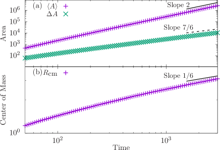
Figure 2: Deviation of some global magnitudes for FPP isochrones with $d_{c}=1$: average radius, area, and center-of-mass deviation. The straight lines in each panel represent the corresponding theoretical expectation for 1D KPZ behavior, see Table 1.

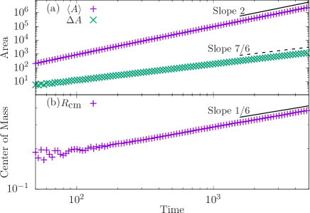
Figure 3: Deviation of some global magnitudes for FPP isochrones with $d_{c}=20$: average radius, area, and center-of-mass deviation. The straight lines in each panel represent the corresponding theoretical expectation for 1D KPZ behavior, see Table 1.

III Numerical results

In this section we will compare our theoretical predictions, collected in Table 1, with numerical simulations of different models which are known to follow FV scaling. We will discuss first-passage percolation (FPP), random metrics, and shadowing models. Besides these models, we have also performed simulations on two flavors of the random deposition model Barabasi for circular clusters, which are shown in Appendix A.

III.1 First-passage percolation

Our first example will be first-passage percolation (FPP) on a square $L\times L$ lattice, which is defined as follows. Each lattice link $k$ has an associated crossing-time, $\left\{t_{k}\right\}$, which are independently identically distributed (i.i.d.) random variables extracted from a certain probability distribution, with cumulative probability function $F(t)$ such that $F(0)=0$. Employing Dijkstra’s algorithm Cormen.90 we find the minimal arrival time at every vertex $i$ starting from the lattice center Cordoba.18 , $\left\{T_{i}\right\}$. Then we determine the ball of radius $R$ as the set of vertices for which $T_{i}\leq R$. We have chosen uniform distributions for the crossing-times with mean $\mu$ and deviation $\sigma$. The balls are then characterized by the crossover length $d_{c}\equiv\mu^{2}/(3\sigma^{2})$. In Fig. 1 (a) and (b) we can see typical profiles using $d_{c}\approx 1$ and $d_{c}=20$. Notice that the average shape is nearly circular in the first case, and similar to a diamond in the second. Yet, the fluctuations are known to correspond to KPZ for all values of $d_{c}$ Villarrubia.20 ; Alvarez.23 .

We have run $10^{4}$ simulations on $L=2401$ FPP lattices, using uniform time distributions with $\mu=5$ and different $d_{c}$. The time evolution of the average and deviation of the area and the CM displacement are shown in Fig. 2 for $d_{c}=1.04$ and in Fig. 3 for $d_{c}=20$. Notice that for this discrete model in particular, the aforementioned global magnitudes are easier to obtain, because they are measured in the bulk. The boundaries of the balls, which are called isochrone curves or isochrones, present some subtle points Alvarez.23 and have been left out from our present numerical study. The solid black lines show the theoretical predictions, extracted from the last column of Table 1 (1D KPZ behavior), and show good agreement with the simulation data.

Figure 4: Expected values and deviations for the global magnitudes for random-metric isochrones: (a) Radius, (b) area, (c) width, (d) center-of-mass displacement, and (e) length. The straight lines in each panel represent the corresponding theoretical expectation for 1D KPZ behavior, see Table 1.

III.2 Random metrics

The FPP problem is a discrete analogue of the more general random metrics problem Santalla.15 . In the latter, we consider a random two-dimensional manifold, flat in average, whose metric tensor presents only short-distance correlations, and obtain the isochrone curves by integrating Huygens’ equation,

$$\partial_{t}\vec{r}=\vec{n}_{g}(\vec{r}),$$ (27)

where $\vec{n}_{g}(\vec{r})$ denotes the local normal to the isochrone at position $\vec{r}$, according to the metric tensor $g$. Both the isochrones and the times-of-arrival present very accurate 1D KPZ scaling from the beginning Santalla.15 .

We have performed 1280 simulations of Huygens’ equation, Eq. (27). Each simulation starts out with a very small ball, with initial radius $0.05$, and propagates it through a random metric field with uniformly distributed eigenvalues $\lambda\in[1/20,1]$, using a time-step $\Delta t=5\times 10^{-3}$. We have obtained the full set of global observables: average radius, area, width, CM displacement, and length, whose time evolutions are shown in Fig. 4, along with the theoretical predictions extracted from Table 1. Notice that, in all the considered cases, the theoretical lines accurately describe the simulation data.

Furthermore, we have checked the length-to-radius ratio, i.e. the value of $2\hat{\pi}$, and the results are shown in Fig. 5. Indeed, the theoretical predictions are once more correct, with the ratio converging to a fixed value whose fluctuations decay as $t^{-1/2}$, as predicted by Eq. (26).

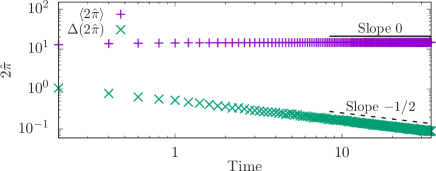
Figure 5: Expected values and variances of the length-to-radius ratio, or $2\hat{\pi}$, for random-metric isochrones, along with the comparison to the theoretical prediction, Eq. (26), for 1D KPZ behavior.

III.3 Shadowing model

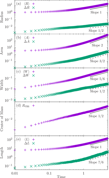
Figure 6: Expected values and deviations for the global magnitudes for the shadowing model: (a) Radius; (b) Area; (c) Width; (d) Center-of-mass displacement; (e) Length.

Motivated by the morphological instabilities of the fronts of growing planar bacterial colonies, shadowing effects may be introduced phenomenologically into the radial KPZ equation, such that each point at the interface moves along the normal direction with a velocity which is proportional to the local aperture angle, i.e. the fraction of rays emanating from the point which do not intersect the interface Santalla.18 ; Santalla.21 . The resulting continuum model is given by the following equation,

$$\partial_{t}\vec{r}=\left(A_{0}+A_{1}K(\vec{r})+A_{a}\Theta_{a}(\vec{r})+A_{n}\eta\right)\vec{n},$$ (28)

where $\vec{r}$ is any interface point, $\vec{n}$ is the local exterior normal, $K(\vec{r})$ denotes the curvature of the interface at that point, $\Theta_{a}(\vec{r})$ is the local aperture angle, and $\eta$ is a zero-average and unit variance, Gaussian, uncorrelated space-time noise. Furthermore, $A_{0}$, $A_{1}$, $A_{a}$, and $A_{n}$ are positive parameters which quantify, respectively, the relative strengths of the average growth velocity of a planar front, surface tension, the dependence on the aperture angle, and fluctuations. For a convex smooth shape, the aperture angle is uniformly equal to $\pi$. The subsequent dynamics tends to make peaks grow faster than valleys, thus giving rise to morphological instabilities. Indeed, in the long run the typical cluster is composed of a set of correlated lobes separated by deep crevices whose angular distance is nearly constant in time. An example can be seen in Fig. 1 (d).

We have performed 500 simulations of Eq. (28) using the same numerical scheme as in Ref. Santalla.18 , for initial radius 1, $A_{0}=0$, $A_{1}=0.1$, $A_{a}=1$, $A_{n}=0.1$, and time-step $\Delta t=10^{-4}$. We have measured the full set of global magnitudes: average radius, area, width, CM displacement, and length. The time evolution of their average and deviation can be found in Fig. 6. Previous work Santalla.18 ; Santalla.21 was able to unambiguously rule out KPZ scaling for this model, even finding traces of nonuniversality both in experiments and in simulations, and very precise values of the critical exponents could not be ascertained for the FV behavior that could nevertheless be confirmed. Yet, our present global measurements agree with the scaling behavior predicted in Sec. II, compatible with (non-KPZ) values for the scaling exponents $\beta\approx 5/6$ and $\zeta=1/z\approx 1/3$, implying $\alpha=\beta z\approx 5/2$.

IV Other statistical properties

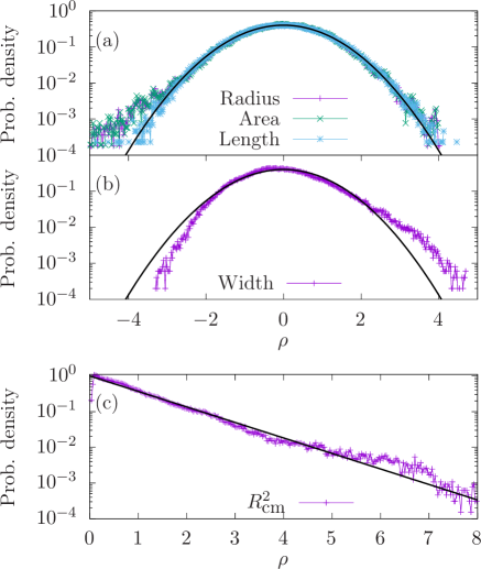
Figure 7: Probability density for the standardized global magnitudes, Eq. (29), considered for the random metrics system; (a) Radius, area and length, along with the unit Gaussian; (b) Squared width, along with an exponential decay, as predicted in other cases in the literature Foltin.94 ; Halpin.15 ; (c) Squared CM displacement, $R_{\text{cm}}^{2}$, along with the $\chi^{2}$-distribution for $k=2$ degrees of freedom (i.e. an exponential decay).

IV.1 Histograms

We may also provide some predictions for the full histograms of some of the global observables considered. Indeed, if the number of patches $n_{P}$ is large, the average radius, the area, and the length can be considered to be the sum or average of a series of i.i.d. random variables. The central limit theorem then predicts that, under very broad circumstances, the probability distribution for the global observables must be Gaussian. In the random metrics case, we have considered the full set of values of the average radius, area, and length, for a given time $t$, substracted their (time-dependent) average and divided by their (time-dependent) deviation so that their average becomes zero and their variance becomes one, i.e., we have defined

$$\rho_{i}={U_{i}-\left\langle U(t)\right\rangle\over\sigma_{U}(t)}.$$ (29)

Then we have plotted the histograms of the full set of values $\rho_{i}$ in Fig. 7 (a), along with the unit Gaussian, showing their correspondence. The prediction is specially good for the length, with some deviation for the radius and area.

In Fig. 7 (b) we show the histogram for the $\rho_{i}$ values corresponding to the square of the global width, which need not be Gaussian. In fact, results associated to the KPZ class in band geometry after saturation show a very skewed histogram with a large-devations exponential decay Halpin.15 , which can be accounted for by considering the behavior of random walks Foltin.94 ; Antal.02 . Our case, which corresponds to circular geometry and is not saturated, also shows a large-deviation exponential decay, as we can see in Fig. 7 (b).

Furthermore, Figure 7 (c) shows the histogram for the squared CM displacements, $R_{\text{cm}}^{2}$, merely normalized to have variance one. In this case, the theoretical prediction is not Gaussian. Indeed, $R_{\text{cm}}^{2}=X_{\text{cm}}^{2}+Y_{\text{cm}}^{2}$, where $X_{\text{cm}}$ and $Y_{\text{cm}}$ can be in turn considered to be Gaussian. Therefore, the sum of squares must follow a $\chi^{2}$-distribution for two degrees of freedom, which is an exponential distribution as we can indeed observe in the plot.

IV.2 Correlations between global magnitudes

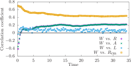
Figure 8: Correlation coefficients, Eq. (30) between some pairs global magnitudes as a function of time, for the random metrics system: width vs radius, area, length, and center-of-mass displacement.

It is interesting to consider whether the sample-to-sample fluctuations of different global magnitudes present correlations. Indeed, it is natural to expect that the fluctuations of the average radius and the area must be strongly correlated, with a smaller (yet positive) correlation between the CM displacement and the interface width.

In order to obtain a theoretical prediction, we consider any two global magnitudes $U$ and $V$, and define their correlation coefficient,

$$r_{UV}\equiv{\left\langle UV\right\rangle-\left\langle U\right\rangle\left\langle V\right\rangle\over\sigma_{U}\sigma_{V}}.$$ (30)

If we assume that the correlator between different magnitudes behaves as [recall Eq. (2)]

$$C_{uv}(\theta,\theta^{\prime})=A_{uv}t^{\phi_{a}+\phi_{b}}\;g_{2}(B_{uv}t^{1-\zeta}\hat{\theta}),$$ (31)

then

$$\left\langle UV\right\rangle-\left\langle U\right\rangle\left\langle V\right\rangle= \int d\theta d\theta^{\prime}\;C_{uv}(\theta,\theta^{\prime})$$

$$\sim {2\pi A_{uv}\over B_{uv}}t^{\phi_{u}+\phi_{v}+\zeta-1}\int_{0}^{\infty}dx\;g_{2}(x),$$ (32)

whose time dependence is the same as that for the product $\sigma_{U}\sigma_{V}$, thus concluding that the correlation coefficients approach time-independent values. This is indeed what we observe in Fig. 8, where we have considered the correlation coefficients between the width and the other four global observables in the random metrics simulations. Notice that the curves for the average radius and the area overlap almost perfectly, because the correlation coefficient between them is close to one.

V Conclusions

In this work we have presented a scaling approach to the sample-to-sample fluctuations of global geometrical observables measured on random planar clusters whose fronts display statistical properties satisfying the Family-Vicsek Ansatz. The chosen observables were the average radius, the area, the width, the center-of-mass displacement, and the length of the clusters. The sample-to-sample deviations of these observables are thus predicted to present power-law dependences with time, with exponents values that can be determined from the Family-Vicsek exponents $\beta$ (growth exponent) and $z$ (dynamical exponent).

We have tested our predictions against several different growth systems: random deposition in two different versions (see Appendix A), first-passage percolation clusters and random metrics isochrones (both belonging to the KPZ universality class), and shadowing dynamics (which does not). In all the considered cases, the predictions met the actual scaling found in the simulations.

We have also addressed the full histogram of the sample-to-sample fluctuations of these global variables. Some of them, such as the radius, area and length, are seen to be Gaussian. However, and in analogy to the case of KPZ growth in a band geometry Foltin.94 ; Antal.02 ; Halpin.15 , the histogram of the width or roughness is not Gaussian, and this remains beyond our present scaling arguments. The center-of-mass displacement follows a $\chi^{2}$-distribution with $k=2$ degrees of freedom, as predicted. Also, the sample-to-sample correlation coefficients between these magnitudes approach time-independent, limiting values, also as predicted.

In principle, our work enables alternative characterizations of the universality class in terms of exponent values, for rough interfaces with an overall, circular symmetry, by employing sample-to-sample fluctuations of global magnitudes associated to the clusters. Indeed, it is possible to obtain both the growth and the dynamical exponents using the fluctuations in two complementary global magnitudes, such as the average radius and the total length. Methodologically, this may turn out to be advantageous in the analysis of e.g. experimental and/or simulation data.

Appendix A Random deposition

The simplest growth model is, indeed, random deposition (RD), which always yields $\beta=1/2$ Barabasi . In a circular framework, we may consider two flavors of the RD class (additional formulations are possible, see e.g. Escudero.11 and related references), depending on the discretization scheme and the treatment of the UV-cutoff. In what we will call model RD-1, we set up a fixed angular discretization with an UV-cutoff $\Delta\theta=2\pi/N$, where $N$ is the number of points. Now, the interface is described by a set of $N$ radial values, $\left\{r_{i}\right\}_{i=1}^{N}$, with $r_{i}=r(\theta_{i})$. At each time-step, we allow each $r_{i}$ to grow independently of the others. In practice, we are imposing that each wedge $\Delta\theta$ remains completely correlated. Therefore, $\xi\sim t$, i.e. the correlated patches grow as fast as the interface itself and $\zeta=1$.

Model RD-2, on the other hand, includes a UV cutoff for length instead of an angular one Rodriguez.11 ; Santalla.14 ; Santalla.15 . Therefore, the length of the correlated patches remains time independent, and $\zeta=0$. The differences between both RD models can be seen in the profiles shown in Fig. 9.

The predictions for the sample-to-sample fluctuations of global magnitudes vary for the two models. We discard the cluster length, because our calculation assumed that the interface was smooth enough at the cutoff scale, which is not the case here. The remaining scaling exponents are shown in Table 2, and have been measured in the numerical simulations shown in Fig. 10. In our simulations we have run $1000$ samples with a growth velocity $v=1$, $\Delta t=0.01$, and unit adaptive UV-cutoff for the RD-2 model. The largest discrepancy between the theoretically expected exponents and those measured in the simulations are found in model RD-2 for the deviations of the average radius and for the CM deviation; in both cases we expect a zero exponent value but we measure $0.13$ approximately, possibly due to limitations in our longest simulation times. Other than this, the predictions seem accurate.

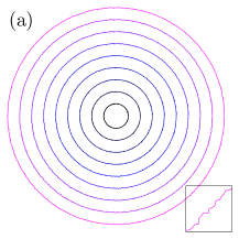
Figure 9: Profiles for the random deposition models discussed in Appendix A: (a) Model RD-1 has a fixed angular cutoff; (b) Model RD-2 has an adaptive cutoff, thus the number of points along the interface grows witht time.

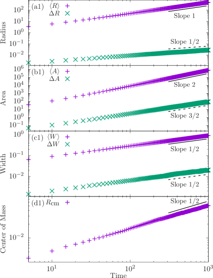
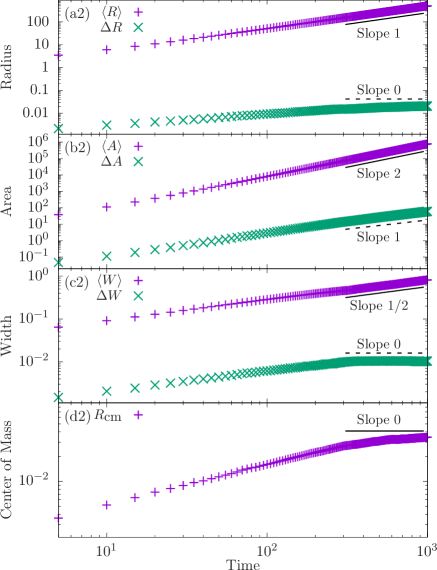
Figure 10: Time evolution of the average and sample-to-sample deviation of global magnitudes from numerical simulations of model RD-1 in panels (a1) to (d1), and of model RD-2 in panels (a2) to (d2). The straight lines in each panel represent the corresponding theoretical expectation, see Table 2. The largest deviations between the numerical data and our scaling predictions are for the radial deviations [panel (a2)] and the CM displacement [panel (d2)] of the RD-2 model. In both cases the expected exponent is zero, while the measured value is approximately $0.13$.

Observable	Scaling exponent	RD-1	RD-2
$\Delta R$	$\beta+(\zeta-1)/2$	1/2	0
$\Delta A$	$\beta+(\zeta+1)/2$	3/2	1
$\Delta W$	$\beta+(\zeta-1)/2$	1/2	0
$R_{\text{cm}}$	$\beta+(\zeta-1)/2$	1/2	0

Table 2: Scaling behavior of different geometric global observables for the RD-1 and RD-2 models. The growth exponent $\beta=1/2$ for both models, but $\zeta=1$ for RD-1 and $\zeta=0$ for RD-2.

References

- (1) A.-L. Barabási and H. E. Stanley, Fractal Concepts in Surface Growth (Cambridge University Press, Cambridge, UK, 1995).
- (2) K. A. Takeuchi, M. Sano, T. Sasamoto, and H. Spohn, Growing interfaces uncover universal fluctuations behind scale invariance, Sci. Rep. 1, 34 (2011).
- (3) S.N. Santalla, J. Rodriguez-Laguna, T. LaGatta, and R. Cuerno, Random geometry and the Kardar–Parisi–Zhang universality class, New J. Phys. 17, 033018 (2015).
- (4) P. Córdoba-Torres, S.N. Santalla, R. Cuerno, and J. Rodríguez-Laguna, Kardar-Parisi-Zhang universality in first passage percolation: the role of geodesic degeneracy, J. Stat. Mech. 063212 (2018).
- (5) S.N. Santalla, J. Rodríguez-Laguna, J.P. Abad, I. Marín, M.M. Espinosa, J. Muñoz-García, and R. Cuerno, Nonuniversality of front fluctuations for compact colonies of nonmotile bacteria, Phys. Rev. E 98, 012407 (2018).
- (6) S. Najem, A. Krayem, T. Ala-Nissila, and M. Grant, Kinetic roughening of the urban skyline, Phys. Rev. E 101, 050301(R) (2020).
- (7) F. Family and T. Vicsek, Scaling of the active zone in the Eden process on percolation and the ballistic deposition model, J. Phys. A: Math. Gen. 18, L75 (1985).
- (8) T. Halpin-Healy and K.A. Takeuchi, A KPZ cocktail-shaken, not stirred… Toasting 30 years of kinetically roughened surfaces, J. Stat. Phys. 160, 794 (2015).
- (9) M. Kardar, G. Parisi, and Y.C. Zhang, Dynamic scaling of growing interfaces, Phys. Rev. Lett. 56, 889 (1986).
- (10) M. Prähofer and H. Spohn, Scale invariance of the PNG droplet and the Airy process, J. Stat. Phys. 108, 1071 (2002).
- (11) I. Corwin, J. Quastel, and D. Remenik, Continuum statistics of the Airy2 process, Comm. Math. Phys. 317, 347 (2013).
- (12) G. Foltin, K. Oerding, Z. Rácz, and R.L. Workman, R.K.P. Zia, Width distribution for random-walk interfaces, Phys. Rev. E 50, R639 (1994).
- (13) T. Antal, M. Droz, G. Györgyi, and Z. Rácz, Roughness distribution for signals, Phys. Rev. E 65, 046140 (2002).
- (14) C. Misbah, O. Pierre-Louis, and Y. Saito, Crystal surfaces in and out of equilibrium: A modern view, Rev. Mod. Phys. 82, 981 (2010).
- (15) N. E. Muzzio, M. A. Pasquale, M. A. C. Huergo, A. E. Bolzán, P. H. González, and A. J. Arvia, Spatio-temporal morphology changes in and quenching effects on the 2D spreading dynamics of cell colonies in both plain and methylcellulose-containing culture media, J. Biol. Phys. 42, 477 (2016).
- (16) S.C. Ferreira Jr. and S.G. Alves, Pitfalls in the determination of the universality class of radial clusters, J. Stat. Mech.: Theor. Exp. P11008 (2006).
- (17) Y. Saito, M. Duffay, and O. Pierre-Louis, Nonequilibrium Cluster Diffusion During Growth and Evaporation in Two Dimensions, Phys. Rev. Lett. 108, 245504 (2012).
- (18) J.M. Hammersley and D.J.A. Welsh, First-passage percolation, subadditive processes, stochastic networks and generalized renewal theory, in Bernoulli, Bayes, Laplace Anniversary Volume, ed. J. Neyman and L.M. LeCam, Springer, p 61 (1965).
- (19) D. Villarrubia, I. Álvarez Domenech, S.N. Santalla, J. Rodríguez-Laguna, and P. Córdoba-Torres, First-Passage Percolation under extreme disorder: from bond-percolation to Kardar-Parisi-Zhang universality, Phys. Rev. E 101, 062124 (2020).
- (20) I. Álvarez Domenech, J. Rodríguez-Laguna, R. Cuerno, P. Córdoba-Torres, and S.N. Santalla, Shape effects in the fluctuations of random isochrones on a square lattice, ArXiv: 2311.01400 (2023).
- (21) S.N. Santalla, J. Rodriguez-Laguna, A. Celi, and R. Cuerno, Topology and the Kardar–Parisi–Zhang universality class, J. Stat. Mech. 023201 (2017).
- (22) E. Ben-Jacob, I. Cohen, H. Levine, Cooperative self-organization of microorganisms, Adv. Phys. 49, 395 (2000).
- (23) T.H. Cormen, C.E. Leiserson, R.L. Rivest, and C. Stein, Introduction to algorithms, The MIT Press (1990).
- (24) S.N. Santalla, and S.C. Ferreira, Eden model with nonlocal growth rules and kinetic rougnening in biological systems, Phys. Rev. E 98, 022405 (2021).
- (25) C. Escudero, Statistics of interfacial fluctuations of radially growing clusters, Phys. Rev. E 84, 031131 (2011).
- (26) J. Rodríguez-Laguna, S.N. Santalla, and R. Cuerno, Intrinsic geometry approach to kinetic surface roughening, J. Stat. Mech. 05032 (2011).
- (27) S.N. Santalla, J. Rodríguez-Laguna, and R. Cuerno, Circular Kardar-Parisi-Zhang equation as an inflating, self-avoiding ring polymer, Phys. Rev. E 89, 010401(R) (2014).