Tessel: Boosting Distributed Execution of Large DNN Models via Flexible Schedule Search

Abstract

Increasingly complex and diverse deep neural network (DNN) models necessitate distributing the execution across multiple devices for training and inference tasks, and also require carefully planned schedules for performance. However, existing practices often rely on predefined schedules that may not fully exploit the benefits of emerging diverse model-aware operator placement strategies. Handcrafting high-efficiency schedules can be challenging due to the large and varying schedule space. This paper presents Tessel, an automated system that searches for efficient schedules for distributed DNN training and inference for diverse operator placement strategies. To reduce search costs, Tessel leverages the insight that the most efficient schedules often exhibit repetitive pattern (repetend) across different data inputs. This leads to a two-phase approach: repetend construction and schedule completion. By exploring schedules for various operator placement strategies, Tessel significantly improves both training and inference performance. Experiments with representative DNN models demonstrate that Tessel achieves up to 5.5$\times$ training performance speedup and up to 38% inference latency reduction.

I Introduction

Deep Neural Network (DNN) models have demonstrated impressive performance across a wide range of domains [22, 19, 31, 43]. As their complexity and depth continue to increase, their size has outpaced the capacity of existing hardware to keep up with their training and inference demands [3, 19]. Consequently, the distributed execution of large DNN models across multiple devices has emerged as a necessary solution to mitigate memory limitations. Specifically, pipeline parallelism [10, 8, 17] becomes one of the most adopted techniques for efficient parallel execution of distributed DNN training and inference [16, 45, 27, 2].

A DNN model consists of computational operators and data tensors, with a training or inferring task iteratively computing the operators over tensors. The execution of each iteration can be defined by a distributed execution plan, which determines spatial placement and temporal schedule of operators among devices. The spatial placement decides whether operators are executed on one or multiple devices, following the temporal schedule that decides per-device execution order of operators.

Both the spatial placement and temporal schedule are critical to the performance of an execution plan. Prior research has extensively explored various spatial placement strategies and demonstrated their effectiveness in practical applications [45, 33, 16, 18]. However, existing practices primarily rely on pre-defined schedules [8, 17, 2], which lag behind the advancements in placement strategies and can lead to inefficiencies (§II).

In this paper, we focus on exploring the temporal schedule for distributed DNN execution under diverse spatial placement strategies. Once the operators’ placement is determined, the task of finding efficient temporal schedules becomes challenging and complex. First, the schedule space is large. To mitigate peak memory costs, a training iteration is usually used to divide numerous input data samples into hundreds or even thousands of independent micro-batches [10, 21], thereby creating a large schedule space during execution. For example, one can execute the micro-batches sequentially, resulting in minimal peak memory but low device utilization due to idle wait time [10]. Alternatively, one can explore more complex schemes by allowing multiple in-flight micro-batches simultaneously [8, 20], leading to better utilization but requiring careful design of sophisticated schedules that can be error-prone. Furthermore, the schedule space can vary depending on the operator placement. For example, a placement scheme may group model operators into consecutive stages, with each stage placed to a distinct device [20]. In such a case, each device is tasked with scheduling the execution of only one stage with different micro-batches. However, an alternative scheme may place multiple stages on the same device [21, 17], which can substantially increase the schedule space, since each device may execute multiple stages following different orders.

Faced with the complexity of the schedule problem, we present Tessel, a system that takes an operator placement strategy as the input and automatically searches for highly efficient schedules for distributed DNN training and inference. We observed that, given the same operator placement, the schedule space for fewer micro-batches is much smaller than for a larger number of micro-batches. After analyzing a large number of efficient schedules, we further observed that efficient schedules often exhibit a repetitive execution pattern, referred to as repetend (§III-C), where only a small portion of time is dedicated to performing non-repetend executions at the beginning and the end. The schedule search space can be significantly reduced by first searching for a repetend within a small number of micro-batches and then extending it to construct the schedule for further micro-batches.

Based on this observation, we introduced a two-phase approach for Tessel to address the schedule problem, consisting of repetend construction and schedule completion. During repetend construction, Tessel searches for an operator set that can form an efficient repetend over a small number of micro-batches (§IV-B). In the second phase, Tessel completes the schedule of warmup and cooldown parts by optimizing the execution time for the remaining micro-batch computations (§IV-C). Finally, the searched schedule is instantiated to the runtime and optimized by inserting non-blocking communication primitives (§IV-D).

The automated search in Tessel facilitates the exploration of schedules for various operator placement strategies and generates highly efficient schedules, including existing ones such as 1F1B [8] or Chimera [17], as well as novel schedules that can significantly improve training and inference performance. Our experiments demonstrate that Tessel achieves up to 5.5$\times$ performance speedup on training language models with large embedding layers, and reduces up to 38% inference latency in multi-modality models such as Flava [31] (§VI). We plan to release Tessel to the open-source community.

We make the following contributions:

• Formulation of the schedule problem for distributed DNN training and inference given various operator placement strategies.

• Introduction of Tessel, which is the first system to efficiently search for high-performance schedules based on the given operator placement strategies.

• Implementation of an end-to-end system that supports instantiating searched schedules for efficient runtime execution.

II Background and Motivation

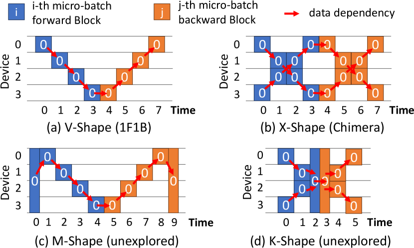
Figure 1: Diverse possible operator placement strategies of one micro-batch. The blue and orange blocks denote forward and backward execution blocks, respectively. The red arrows denote data dependency between different blocks.

For distributed DNN training and inference, previous works [8, 17, 18, 37] have effectively explored flexible placement strategies for execution plans, showcasing their effectiveness in many real-world scenarios. Figure 1 uses a single micro-batch to illustrate several typical placement strategies, such as (a) grouping operators into execution blocks and sequentially placing them among devices [8], (b) distributing them on distinct devices to form a bi-directional pipeline execution [17], (c) employing a more advanced strategy to distribute memory-intensive operators across all devices [18], or (d) leveraging model architecture, e.g., 2-branch, to place operators from independent branches on different devices [37]. However, all these solutions employ pre-defined schemes such as 1F1B [8, 20] and Chimera [17] to schedule multiple micro-batches, leaving the temporal schedule largely unexplored.

Furthermore, the emergence of large DNN models has introduced a significant increase in diversity, such as large embedding layers [22, 44] in multilingual models, and multiple independent branches in multi-modal models [31, 39, 14]. Such diversity poses challenges to existing predefined schedules but, also presents new opportunities to further improve performance. Figure 2 shows the training performance of a GPT model with a large embedding layer using the 1F1B schedule following the Piper [33] policy. With the increasing number of layers, computations on each device become increasingly imbalanced. The slowest stage is 3.4$\times$ slower than the fastest stage for the 40-layer GPT, leading to significantly lower device utilization in the first stage. This is because the large embedding layer consumes a significant amount of memory but requires only little computation cost. The large embedding layer requires at least two GPUs to fit in, leaving little room for co-locating other computation-intensive layers, i.e., transformer [36] layers. As a result, many computation-intensive layers can only be placed on the remaining two GPUs, leading to computational imbalance and performance drop.

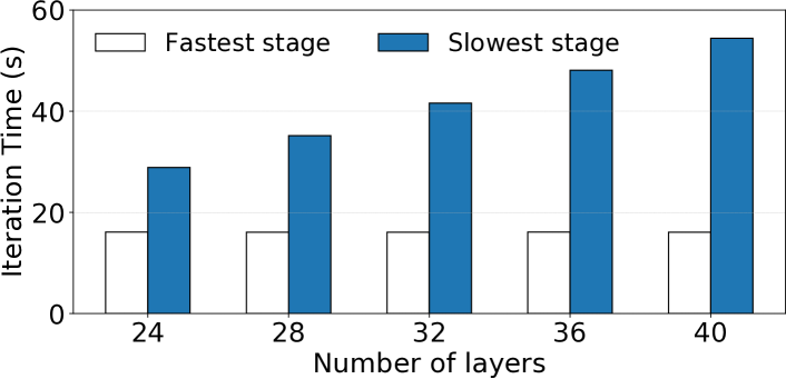
Figure 2: Training performance of GPT model with different number of layers. (Embedding vocabulary size 768k, layer from GPT 6.7B, on 4 V100-32GB GPUs).

A more advanced operator placement strategy such as the one shown in Figure 1(c) may better fit this model, where the large embedding layer is distributed across all devices, allowing computation-intensive layers to share devices with the embedding layer. This can help alleviate the memory bottleneck, achieving a more balanced stage computation cost. However, predefined schedules such as 1F1B face challenges in direct application as it conflicts with the assumption that different stages are placed on distinct devices. While it’s possible to manually adapt the 1F1B schedule to accommodate this placement strategy (§VI), these schedules would still suffer from low device utilization due to factors such as data dependency waiting.

The diversity in model-aware operator placements also highlights the importance of tailored schedules. Multi-modal models [31, 14], for instance, treat distinct input modalities as separate branches, enabling a new placement strategy (i.e., Figure 1(d)) that concurrently executes each branch on different devices to reduce latency. However, there is no out-of-the-box schedule for such placement strategy, making it necessary to find corresponding schedules.

III Problem Formulation And Insights

Notation	Meaning
$N$	Number of micro-batches
$D$	Number of devices
$M$	Memory capacity of each device
$K$	Number of blocks in each micro-batch
$B_{i}^{n}$	$i$-th execution block on $n$-th micro-batch
$\mathbb{B}$	Set of all blocks in a schedule
$t_{B}$	Time cost of executing block $B$
$s_{B}$	Start time of executing block $B$
$d_{B}$	Device(s) to execute block $B$
$m_{B}$	Memory cost of executing block $B$
$B_{i}\rightarrow B_{j}$	Data dependency where block $B_{j}$ depends on block $B_{i}$

TABLE I: Notations used in this paper.

To better understand the schedule problem, we first formulate it as the problem of determining an optimal schedule for distributed DNN training or inference. We then highlight the challenges posed by the large search space inherent in this problem, which makes naive exhaustive search infeasible. Finally, we present our key insights into reducing the search space during efficient schedules discovery.

III-A Problem Definition

Consider an iteration of DNN model training that comprises $N$ independent micro-batches. The DNN model is distributed across $D$ homogeneous devices, each with the same memory capacity of $M$. The operator placement for each micro-batch is predetermined, and the execution of each micro-batch $n(0\leq n<N)$ can be represented as the execution of $K$ blocks denoted as $B_{i}^{n}$, where $0\leq i<K$. Each block corresponds to a sub-set of operators on a device or a group of devices (utilizing tensor parallelism). Figure 1 illustrates several possible scenarios of operator placement strategies. Each block $B$ has an associated execution time $t_{B}\in\mathbb{Z}^{+}$ and memory consumption $m_{B}\in\mathbb{Z}$. Without losing generality, we use integers ($\mathbb{Z}$) to express both $t_{B}$ and $m_{B}$ to maintain compatibility with tools such as the Z3-solver [7]. Certain blocks, such as backward computation, may exhibit negative memory consumption, indicating the release of memory after execution. The execution of each block can be determined to start at time $s_{B}(s_{B}\geq 0,s_{B}\in\mathbb{Z})$. Table I presents a summary of the notations used in this paper.

Exclusive execution constraints.   As a common practice [8, 17], we adhere to the exclusive execution of blocks on each device. This means that each device executes only one block at a time, as the operators in large DNN models typically saturate the device.

Memory constraints.   An executable schedule must satisfy memory constraints. During a typical training iteration, executing a micro-batch consists of both the forward and backward computation. The forward computation involves the creation of tensors, which in turn consumes memory. Conversely, the backward computation involves the release of previously created tensors, thereby freeing up memory space. As a result, the careful arrangement of block execution can have a significant impact on memory utilization, especially when dealing with a large number of micro-batches, which can amplify the consequences of sub-optimal arrangements.

Data dependency constraints.   Given the operator placement strategy, individual blocks typically exhibit data dependencies, meaning that the completion of prior dependent blocks is a prerequisite for the start of subsequent blocks. This ensures the correct flow of data and computations throughout the DNN models. A valid schedule must strictly follow data dependency to preserve the semantics of the DNN model.

Objective.   The primary objective in exploring an efficient schedule is to minimize the total execution time by searching the start time of each block while adhering to the above constraints. The execution time can be quantified as the time required to complete the execution of the last block among all the blocks ($\mathbb{B}$) within the schedule. Thus, the optimization goal can be formulated as follows, taking into account the aforementioned constraints:

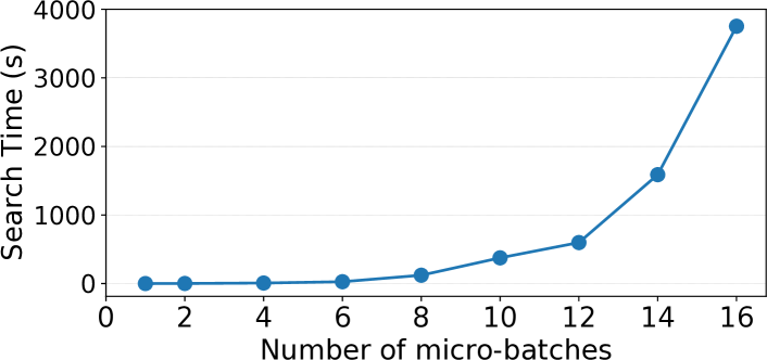
Figure 3: Schedule search time of V-Shape placement with different number of micro-batches.

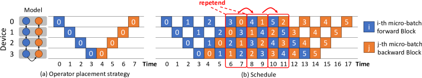
Figure 4: One micro-batch execution from (a) model operator placement, is extended into (b) 6 micro-batches with 1F1B schedule.

minimize $$\quad\underset{B\in\mathbb{B}}{\max}\quad(s_{B}+t_{B})$$ (1)

subject to:

[1] $$\quad\min(s_{B_{i}}+t_{B_{i}},s_{B_{j}}+t_{B_{j}})\leq\max({s_{B_{i}},s_{B_{j}}}),$$

$$\quad\forall B_{i},B_{j}\text{ if }i\neq j,d_{B_{i}}=d_{B_{j}}$$

[2] $$\quad M\geq\underset{\begin{subarray}{c}d\in[0,D)\\ \tau\in[0,+\infty)\end{subarray}}{\max}(\sum_{B\in\mathbb{B}_{\tau}^{d}}{m_{B}}),$$

$$\quad\text{where}\quad\mathbb{B}_{\tau}^{d}=\{B\mid d_{B}=d,s_{B}\in[0,\tau)\}$$

[3] $$\quad s_{B_{i}}+t_{B_{i}}\leq s_{B_{j}},\quad\forall B_{i},B_{j}\text{ if }B_{i}\rightarrow B_{j}$$

In the above, item [2] calculates the peak memory of a device by cumulatively summing the memory of blocks following their execution order, with the maximum value considered as the peak memory. Note that the communication between data-dependent blocks incurs a relatively small cost compared to block execution [45]. Hence, we have omitted it in the schedule.

The schedule problem naturally supports the combination of existing tensor and data parallelisms [34, 30], where operator placement strategies can determine the mapping of blocks to multiple devices for concurrent execution. Given the focus of this paper on efficient schedule searching, we have simplified the presentation of schedules in our figures.

III-B Problem Space

This type of schedule problem is known to be NP-hard [40]. The complexity of the problem grows exponentially as the number of micro-batches increases, due to the independence of blocks among different micro-batches, i.e.,

$$B_{i}^{m}\nrightarrow B_{j}^{n},\quad\forall i,j\in[0,N)\text{ if }m\neq n$$ (2)

Such independence leads to the possibility of arbitrary execution order on these blocks for each device. In practical scenarios, where the number of micro-batches can range from hundreds to thousands [21], the search space becomes prohibitively large to explore using brute-force methods.

To illustrate this challenge, we begin with a GPT model and follow the conventional approach of sequentially placing its operators onto 4 devices, as depicted in Figure 1(a). We employ the Z3-solver [7] to encode and solve the schedule problem, aiming to identify the optimal schedule as the number of micro-batches increases. For simplicity, we assign an execution time of 1 to each forward block and 2 to each backward block. Figure 3 shows the results of the search time with an increasing number of micro-batches. It is evident that as the number of micro-batches grows, the search time increases significantly. In fact, it takes 3752 seconds to complete the search for only 16 micro-batches, indicating that it becomes impractical to search for the optimal schedule when dealing with hundreds or even thousands of micro-batches.

Consequently, it is necessary to address the challenges brought about by the large search space.

III-C Key Insights

By carefully checking many efficient schedules, we observed that: 1) efficient schedules usually exhibit repetitive cycles, wherein the same computations are periodically performed but over different micro-batches; 2) repetitive cycles, referred to as repetend, only involves a small number of micro-batches; 3) the repetend occupies most of the time, especially when the number of micro-batches is large, with a small warmup phase in the beginning and a cooldown phase in the end.

Repetend.   Figure 4 demonstrates the 1F1B schedule on 4 devices. The red boxes show 3 repetends, with the same execution repetitively performed. For example, comparing steps 8-9 with steps 6-7, each device executes the same blocks, except with every micro-batch index increased by one.

Schedule generalization.   We found that if the micro-batch indices between consecutive repetends increase by exactly one, it is possible to extend the repetend schedule to accommodate any number of micro-batches. To illustrate this, consider extending the 6-micro-batch 1F1B schedule in Figure 4 to 7 micro-batches. This can be achieved by replicating the repetend of steps 10-11 while increasing the micro-batch indices of each block in the repetend by one. The blocks originally following step 12 would be shifted by the width of the repetend accordingly, with each block also increasing its micro-batch index by one.

Based on these observations, we can simplify the problem by transforming the search for a full schedule for all micro-batches into a repetend search that involves much fewer micro-batches. Subsequently, it can schedule any large number of micro-batches by extending the efficient repetend and incorporating a proper warmup and cooldown phase schedule.

IV Design

Following the above insights, we present Tessel, a system that supports automated search for efficient schedules given operator placement strategies.

IV-A Tessel Overview

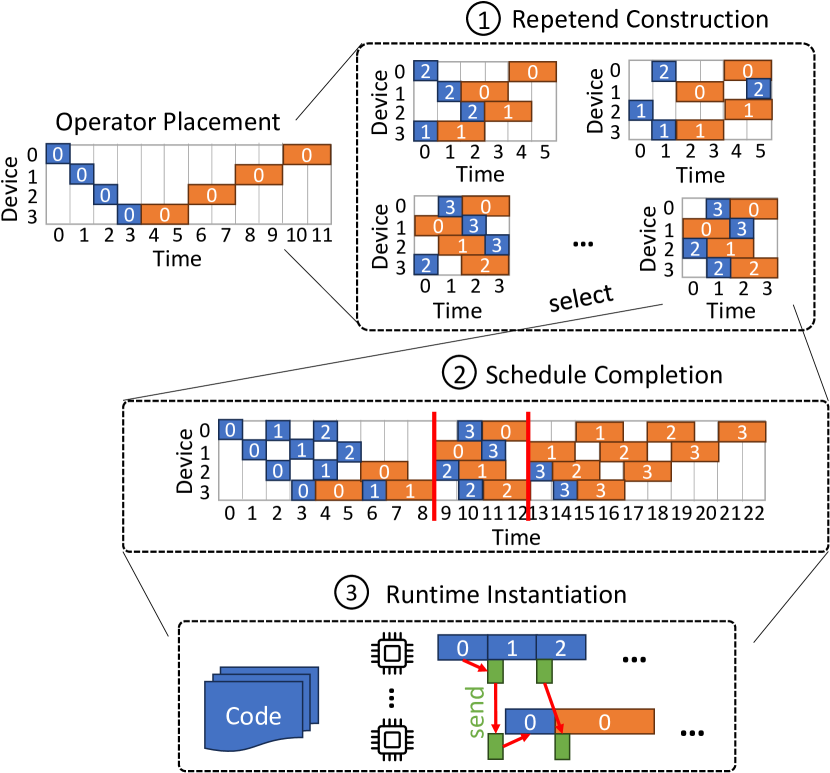
Figure 5: Tessel overview.

Figure 5 illustrates the overview of Tessel. Tessel takes the operator placement strategy and memory budget as inputs. Within the system, Tessel employs three phases for an end-to-end automated search and execution: repetend construction, schedule completion and runtime instantiation, where the first two phases search for an efficient schedule and the last phase instantiates the schedule to runtime for real execution.

Given an operator placement strategy, in repetend construction, Tessel firstly samples all possible blocks from a small number of micro-batches ($N_{R}$) that can form a repetend, and then picks the one with the lowest execution time. Then, given the selected repetend, Tessel completes its warmup and cooldown phase by searching for the time-optimal schedule on the remaining blocks, and extends the schedule to the desired number of micro-batches ($N$). Finally, according to the searched schedule, Tessel inserts communication primitives and generates executable code for each device for runtime.

IV-B Repetend Construction

Given the substantial number of micro-batches, the repetend is repeated numerous times and covers the major portion of iteration time, thus dominating performance.

Block set of repetend.   Through further investigation, we identified a necessary condition for a repetend: a repetend must consist of a full set of blocks in the model, irrespective of their micro-batch indices. For example in Figure 4, step 6-7 is a repetend that contains all blocks to complete the computation of a micro-batch, disregarding the micro-batch indices associated with the blocks. Therefore, blocks of a repetend can be expressed as:

$$\mathbb{B}_{repetend} =\{B_{0}^{n_{0}},B_{1}^{n_{1}},...,B_{K-1}^{n_{K-1}}\},$$ (3)

where $$\quad{n_{0},...,n_{K-1}}\in[0,N_{R})$$

Space pruning.   Constructing a repetend from $N_{R}$ micro-batches leads up to $(N_{R})^{K}$ potential repetends, which still presents a large space. Fortunately, we identified two key properties that can significantly reduce the search space:

Property IV.1

For any schedule, there exists a same-performance schedule of blocks $\mathbb{B}$, $\forall B_{i}^{m},B_{i}^{n}\in\mathbb{B},m<n\text{ if }s_{B_{i}^{m}}<s_{B_{i}^{n}}.$

Property IV.2

$\forall B_{i}^{m},B_{j}^{n}\in\mathbb{B}_{repetend}$, $m\geq n$ if $B_{i}^{0}\rightarrow{}B_{j}^{0}$.

Property IV.1 exploits the symmetry of all micro-batches, such that switching micro-batch indices for blocks doesn’t affect the performance of the schedule. Thus, we can deduplicate symmetric schedules by focusing only on those where micro-batch indices monotonically increase over time for each block.

Property IV.1 further leads to Property IV.2. Within a repetend, we discovered that if $B_{i}$ has data dependency on $B_{j}$ inside one micro-batch, the micro-batch index assigned to $B_{i}$ should not be smaller than the one assigned to block $B_{j}$. This enables a pruning strategy, constraining the assignment of micro-batch indices to a sequence of dependent blocks in descending order.

In addition to the pruned space, Property IV.1 indicates that larger $N_{R}$ can potentially lead to larger peak memory usage. As illustrated in the left of Figure 6, device 0 needs to execute 4 forward blocks ($B^{0}\sim B^{3}$) prior to this repetend, while no backward block is executed since the repetend includes the first backward block with micro-batch 0. Given the limitation imposed by peak memory usage, our search strategy begins with a small number of micro-batches ($N_{R})$, and gradually increases it until we reach the memory capacity constraints.

Repetend performance.   Different repetends lead to varying execution performance, as illustrated in Figure 5 \footnotesize1⃝. Their performance mainly differs in device idle time, which can be attributed to the presence of data dependency and memory constraints. A block can only start after all its data-dependent blocks are finished, and the memory constraints might require a device to wait until a backward block releases memory, even if other forward blocks are ready for execution.

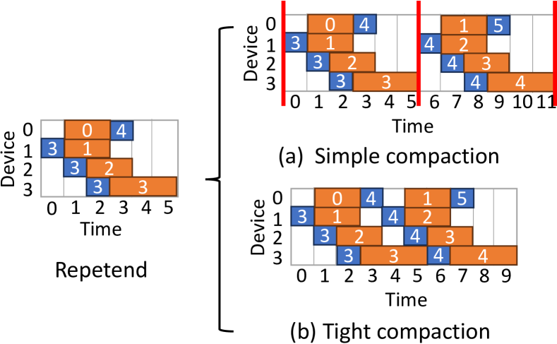
Figure 6: Two ways of compacting neighboring repetends. The repetend is based on a V-Shape operator placement.

Considering the idle time, the execution time of a repetend can be easily evaluated from its first block to the last one. However, this estimation is not precise when certain idle time slots at the end of a repetend can be utilized by a frontier block in the subsequent repetend. Figure 6 demonstrates this case. In Figure 6(a), the repetend is repeated immediately after the completion of the previous repetend. However, we can optimize this pattern by initiating the next repetend as soon as the dependent blocks are finished, rather than waiting for the entire previous repetend to finish. Figure 6(b) shows this approach, where the subsequent repetend starts at time slot 4, as it no longer needs to wait for the completion of the previous repetend due to the timely completion of its dependent blocks by slot 4. This results in a tighter compaction between repetends, effectively reducing device idle time and enhancing overall schedule efficiency.

Therefore, we incorporated the above-mentioned overlapping nature to evaluate repetend performance more accurately, decomposing its time into execution time $E_{R}$ and wait time $W_{R}$. On a device, execution time refers to the duration from the start of the execution of the first block to the completion of the last block, with potential device idle time incorporated. On the other hand, wait time corresponds to the idle time between two consecutive repetends. The efficiency of a repetend determined by the device with the longest time. Therefore, the overall repetend performance ($t_{R}$) can be summarized as:

$$t_{R} =\max_{d\in[0,D)}(E_{R}^{d}+W_{R}^{d}),$$ (4)

$$\text{where}\quad E_{R}^{d} =\max_{B_{i}\in\mathbb{B}_{d}}(s_{B_{i}}+t_{B_{i}})-\min_{B_{i}\in\mathbb{B}_{d}}s_{B_{i}},$$

$$\text{where}\quad\mathbb{B}_{d} =\{B_{i}\mid d_{B_{i}}=d\}$$

$W_{R}$ can be calculated by traversing the execution blocks of the succeeding repetend and determining their earliest starting time based on their between-block data dependencies.

Efficient repetend search.   To find the optimal schedule of the repetend, i.e., the shortest execution time of repetend $t_{R}$, we leveraged Z3-solver [7] to encode the schedule problem and minimize $t_{R}$ (§V). For the memory constraints, by analyzing the micro-batch indices assigned to the blocks in repetend, we can learn the blocks that need to be executed prior to the repetend, and infer the memory usage at the entry of the repetend. Based on this information, we can set the memory constraints for the repetend during the search.

IV-C Schedule Completion

To create a complete schedule, we need to include the warmup and cooldown phases alongside the repetend. Specifically, if the repetend involves a total of $N_{R}$ micro-batches, for any block $B_{i}^{r}$ within the repetend ($\mathbb{B}_{repetend})$, the warmup phase should comprise the blocks defined as:

$$\mathbb{B}_{warmup}=\{B_{i}^{n}\mid\forall B_{i}^{r}\in\mathbb{B}_{repetend},0\leq n<r\}$$ (5)

Similarly, the cooldown phase should include the blocks:

$$\mathbb{B}_{cooldown}=\{B_{i}^{n}\mid\forall B_{i}^{r}\in\mathbb{B}_{repetend},r<n<N_{R}\}$$ (6)

Time-optimal search.   We also employ Z3-solver to perform an optimal search for both the warmup and cooldown phases independently. The objective of this search is to minimize the execution time. The same objective and constraints of this search refer to Equation 1. Note the memory constraints in the cooldown phase will be adjusted accordingly given the execution blocks in the warmup and repetend phases.

Input: Operator placement strategy $OPS$

Input: Memory constraints $M$

Output: General Schedule $schedule$

1

// init the upper bound of repetend time

2 optimal $\leftarrow 0$

3 for $B_{i}\in$ $OPS$.blocks do

4       optimal $\leftarrow$ optimal + $t_{B_{i}}$

5      

6

7schedule $\leftarrow$ None

8 lower_bound $\leftarrow$ GetLowerBound($OPS$)

9

10inflights $\leftarrow$ CalMaxInflight($OPS$, $M$)

11

12for $N_{R}\leftarrow$ 1 to inflights do

13       for repetend $\leftarrow$ IterRepetendBlocks($OPS$, $N_{R}$) do

14             $sched_{R}\leftarrow$ RepetendSolver(repetend, $M$)

15             $t_{R}\leftarrow$ RepetendTime($sched_{R}$)

16            

17            if $t_{R}\geq optimal$ then

18                   continue

19             optimal $\leftarrow$ $t_{R}$

             // get warmup and cooldown blocks

20             warmup $\leftarrow$ GetWarmupBlocks(repetend, $N_{R}$)

21             cooldown $\leftarrow$ GetCooldownBlocks(repetend, $N_{R}$)

22            

            // solver for time-optimal plan

23             $sched_{W}\leftarrow$ TimeOptimalSolver(warmup, $M$)

24             $sched_{C}\leftarrow$ TimeOptimalSolver(cooldown, $M$)

25            

            // compose to the general plan

26             $schedule$ $\leftarrow$ Concat($sched_{W}$, $sched_{R}$, $sched_{C}$)

27            

            // early exit

28             if $t_{R}$ = lower_bound then

29                   return $schedule$

30            

31      

32return $schedule$

Algorithm 1 Tessel schedule search.

Putting it altogether.   Algorithm 1 shows the overall search algorithm, given the operator placement strategy $OPS$ and memory constraints $M$ as inputs. The algorithm begins by initializing the upper bound (optimal) and lower bound of the repetend execution time (Lines 1-5). The function GetLowerBound computes the lower bound of the repetend by summing the execution times of the blocks assigned to each device of one micro-batch and selecting the maximum value across all devices. Additionally, based on the operator placement strategy, the algorithm determines the maximum number of in-flight micro-batches that can be executed within the memory constraints (Line 6).

The search algorithm then follows the strategy outlined in §IV-B. It initiates the search by considering a smaller number of micro-batches $N_{R}$ within the repetend (Line 7). The algorithm then iterates over all possible assignments of micro-batch indices to the blocks (IterRepetendBlocks), following the pruned strategy outlined in Property IV.2 (Line 8). Within each iteration, the solver is employed to search for the optimal schedule for the repetend (Lines 10-13).

Upon discovering a more efficient repetend, the algorithm proceeds to complete the schedule. Firstly, it identifies the warmup and cooldown blocks following §IV-C (Lines 14-15), and then it utilizes the solver to find the time-optimal schedule for both phases (Lines 16-17). Finally, the three phases—warmup, repetend, and cooldown—are concatenated (Concat) to form the best schedule (Line 18). This iterative procedure continues until the lower bound is reached or the memory constraints are exceeded (Lines 19-21).

IV-D Runtime Instantiation

The obtained general schedule serves as a blueprint that needs to be instantiated into executable code during runtime. The schedule solely specifies the per-device execution order of blocks, without addressing the communication necessary for exchanging tensors across devices between blocks.

Inserting communication operations between execution blocks presents two challenges. Firstly, it is crucial to ensure the order of communication operations, as the mis-ordering of send and receive pairs can lead to deadlocks in existing hardware. Secondly, existing solutions typically rely on blocking communication, where devices must wait until the tensors are finished to move from one device to another. While this approach works well for existing schedules such as 1F1B or GPipe, it may not be suitable for all scenarios in Tessel. In some cases, it may be infeasible to find a suitable time at which the devices involved in the communication can simultaneously finish executing their respective blocks.

Topological sort.   To address the first challenge, we first perform a topological sort [13] on the schedule. The output of this sort is a global sequence of execution blocks, where blocks of sharing the same starting time are placed consecutively in the sequence and follow the per-device block execution order determined by the schedule. Then, we treat each pair of send and receive primitives as a single operator and place them right after the time slot that produces the corresponding tensor. During execution, each device executes the assigned blocks and communication primitives in accordance with this ordered sequence. In this way, we can guarantee a consistent execution order for pairs of send and receive communications, avoiding the risk of mis-ordering and potential deadlocks.

Figure 7: Non-blocking communication. The green blocks indicate the communication operators of send (S) and receive (R).

Non-blocking communication.   In order to enhance device utilization and mitigate potential performance degradation caused by blocking communication, we adopt a non-blocking communication pattern. Figure 7 demonstrates the optimization process. Suppose a tensor is generated from a forward block on device 0 and needs to be sent to device 1. As illustrated in Figure 7(a), the execution of the next block has to wait until the data movement by the peer device is completed, resulting in significant idel time for device 0. By employing non-blocking communication, as shown in Figure 7(b), the send and receive operations are executed concurrently with the execution blocks. As a result, the execution of blocks is not impeded by communication operations that are not dependent on them. This approach allows for more efficient utilization of device resources, as execution blocks can progress independently of communication operations that do not have direct dependency on them.

IV-E Discussion

Optimality.   It is important to note that the problem is known to be NP-hard, which implies that finding optimal solutions is computationally infeasible in general. Consequently, Tessel doesn’t guarantee the discovery of optimal solutions. For instance, the search algorithm employed in our approach doesn’t explicitly consider the opportunities arising from jointly optimizing the warmup, repetend, and cooldown phases. However, Tessel works under the assumption that the number of micro-batches is sufficiently large, thereby ensuring that the repetend phase dominates the overall execution. While our approach may not achieve global optimality, it aims to identify efficient schedules that are effective in practice, given the constraints and computational complexity of the problem.

V Implementation

We implemented Tessel based on PyTorch [24]. Tessel takes a DNN model (captured by TorchScript [35]) as well as its operator placement strategy, and automatically searches for efficient schedules with device memory constraints. Then, Tessel generates per-device PyTorch code following the searched schedule together with inserted communication primitives.

Solver implementation.   Z3-solver [7] is a highly efficient Satisfiability Modulo Theories (SMT) solver known for its effectiveness in solving complex constraint satisfaction problems. We rely on Z3-solver to identify the best schedules. In our implementation, each block is associated with a variable (z3.Int) that represents its starting time. To encode the memory constraints, for each device, we traverse the timeline, cumulatively summing the memory cost and updating the peak memory usage by checking the existence of a block on a time slot using z3.If. To determine the optimal schedule, we employ a binary search approach, iteratively checking whether a given objective value can be satisfied.

Lazy search optimization.   The repetend phase search involves only 1 micro-batch’s blocks whereas the warmup and cooldown phases together comprise ($N_{R}-1$) micro-batches’ blocks. Consequently, the warmup and cooldown phases inherently require more time for searching compared to the repetend phase. To mitigate this cost, we implement a lazy search optimization that consolidates the warmup and cooldown phase searches into a one-time process. This is achieved by checking the existence of valid schedules for the warmup and cooldown phases (i.e., by replacing each time-optimal search with a single satisfiability check in Lines 16-17 of Algorithm 1) once a better repetend is identified. Then after the traversal of all possible repetends, Tessel proceeds to search for time-optimal schedules for the warmup and cooldown phases according to the best repetend. This approach significantly reduces the overall search time without changing the searched results.

Non-blocking communication.   Non-blocking communication is performed on a separate GPU stream, distinct from the stream used for computation. To ensure that the tensors being communicated are completed before the execution of blocks that require them, we developed a global message manager to coordinate the communication. Specifically, every non-blocking communication primitive submits the tensor instance and the corresponding communication handler to the message manager. Subsequently, prior to executing each block, the necessary tensor communications are awaited to ensure their completion. This mechanism guarantees the arrival of the required tensors before the execution of dependent blocks.

VI Evaluation

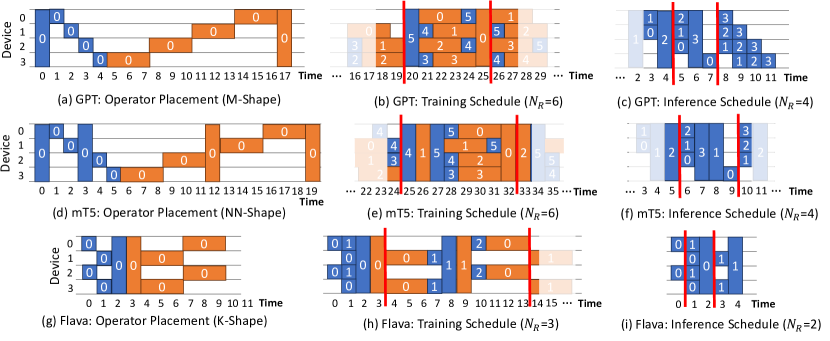
Figure 8: Searched schedules of various models. Each row represents one model of its placement strategy, training and inference schedules from left to right. The blue and orange blocks represent forward and backward blocks, respectively. The number in each block is the micro-batch index. The execution blocks between red bars are repetends.

We evaluated Tessel using a comprehensive approach, beginning with the presentation of the searched schedules in the context of diverse operator placement strategies and models [25, 43, 31]. Subsequently, we conducted ablation studies to examine the obtained results with respect to various factors. Furthermore, we compared the end-to-end training and inference performance of the schedules [8, 17] predominantly employed in practice. Finally, we performed a detailed analysis of the end-to-end performance breakdown.

VI-A Experiment Setup

The evaluation was conducted on a 4-server cluster composed of 32 NVIDIA V100-32GB GPUs. Each server has 40-core Intel(R) Xeon(R) CPU E5-2698 v4 CPUs and 8 GPUs connected through NVLinks. Servers are interconnected via a 100 Gbps Infiniband network. The servers are equipped with NCCL v2.14, PyTorch v1.13 and Z3-solver v4.12.

Models.   We evaluate Tessel using three popular DNN models from various domains, including language and vision: 1) GPT model [25], which is a popular model composed of homogeneous transformer layers [36]; 2) mT5 model [43], which is a multi-language encoder-decoder model, consisting of distinct types of attention blocks. During training, its encoder and decoder parts require access to a shared, large embedding table. For GPT and mT5, we followed the recent trend [44, 22] in multi-language scenarios by setting a larger embedding vocabulary size. 3) Flava model [31], which is a multi-modal model that co-considers language and vision. It incorporates separate text and vision encoders as two distinct branches, and the results of these encoders are jointly computed in a cross encoder. Similar with Megatron-LM [16] and Alpa [45], we scale up the model with the total number of GPUs.

Operator placement.   In Tessel, we adopted more advanced placement strategies for each model and search schedules accordingly. These advanced strategies include distributing memory-intensive operators to all devices for all models and, for Flava, placing independent branches on distinct devices [37]. Figure 8(a,d,g) illustrates the operator placement strategies for GPT, mT5, and Flava, corresponding to M-Shape, NN-Shape, and K-Shape, respectively. Specifically, we applied full-device tensor parallelism for large embedding layers of GPT and mT5, and cross-encoder layers of Flava. For the remaining operators, we further combined data and tensor parallelism within each block for all operator placement strategies, leveraging Piper [33], a state-of-the-art solution that employs dynamic programming, to search optimal configurations for these parallelisms within memory constraints.

Baselines.   We compared Tessel with three Piper-based baselines employing different schedules: 1) 1F1B [8], a popular schedule in current practice that is based on a V-Shape operator placement; 2) Chimera(-direct) [17] which leverages the X-Shape operator placement; 3) 1F1B+ which adapts the 1F1B schedule to incorporate the same advanced placement strategies used in Tessel. To achieve this, we inserted the distributed operators closely to their neighboring operators within the 1F1B schedule, denoting it as 1F1B+.

For all baselines and Tessel, we additionally employed the widely adopted recompute [4] technique to save memory for training. Following common practice [45, 21], we enabled recompute on every transformer layer during training.

VI-B Searching Results

The recompute technique typically results in triple the amount of time for backward computation compared to forward computation [21]. In our evaluation of schedule efficiency, we assumed that each device has a balanced computation workload.

Model	1F1B	Chimera-direct	1F1B+	Tessel
GPT	0%	20%	25%	0%
mT5	0%	20%	20%	0%
Flava	0%	20%	$\times$	0%

TABLE II: Bubble rate of each training schedule considering numerous micro-batches. ’$\times$’ indicates no straightforward adaptation of 1F1B to the given placement strategy.

Training and inference schedules.   Figure 8 displays the operator placement strategies for each model, as well as the discovered schedules for both training and inference. The schedules are formulated using only a small number of micro-batches (up to 6), but they can be generalized to accommodate any large number of micro-batches. Tessel finds schedules that can all achieve full device utilization during repetend computation for both training and inference. It’s worth noting that the compact mechanism (§IV-B) of repetends enables Tessel to discover more flexible repetends, such as those shown in Figure 8(c, f, h), which may appear to have device idle time but can actually be reduced during runtime. Interestingly, in most cases, by simply excluding the execution of backward blocks within the training schedules, we find that the training and inference schedules can share the same execution schedule during the final runtime, despite having different representations of repetends. This indicates that the inference schedules can be easily obtained by selectively excluding the execution of backward blocks and their corresponding communication operations from their training schedules.

Schedule efficiency.   We evaluated the schedule efficiency using bubble rate [30], a common metric calculated by the occupation of device idle time during the entire execution. Table II presents a comparison between Tessel and three other baselines. While Tessel shares the same placement strategy as 1F1B+, it can search for more efficient schedules. Although 1F1B can achieve zero bubble rate under its V-Shape placement strategy, it may suffer from inefficiency due to workload imbalances during real runtime (§VI-D).

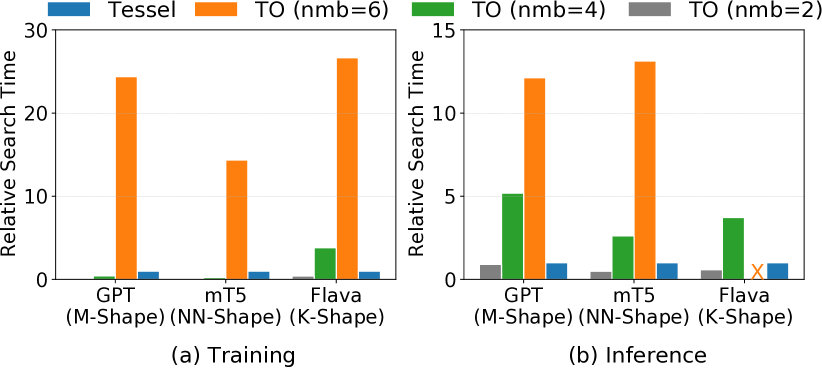
Figure 9: Search cost of TO normalized by Tessel time. ‘$\times$’ denotes value exceeding 10k.

Search cost.   To demonstrate Tessel’s efficient search process over a large schedule space, we compared the search time with the time-optimal search (§II) approach, referred to as TO. Since it is impractical to use TO to search schedules with a large number of micro-batches, we ran TO with different small numbers of micro-batches (nmb) and compared the search time with Tessel. Figure 9 illustrates the results, which show that Tessel significantly reduces search time compared to the baseline solution, indicating its efficiency. While Tessel does not guarantee optimal search results, we observed that when we extended the searched schedules of Tessel to the same number of micro-batches searched by TO, the resulting schedules exhibited the same bubble rates, e.g., both TO and Tessel reached 20% of the bubble rate of NN-Shape for 6 micro-batches, considering both warmup and cooldown phases. This observation suggests that Tessel is able to achieve close-optimal solutions in the majority of cases.

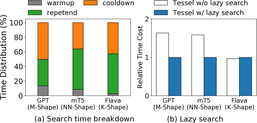
Figure 10: Search time breakdown with lazy search optimization.

Search time breakdown.   We further conducted a breakdown of the search time to study the cost distribution of different phases in Tessel. On average, Tessel spends 147.3 seconds to finish the search. Figure 10 (a) shows the time distribution. We made several observations: 1) Teh cooldown phase tends to require more search time than the warmup phase due to the larger number of blocks in the former phase; 2) Despite the warmup and cooldown phases having more blocks than the repetend phase, their search time remains comparable to that of the repetend phase. This is primarily attributed to the application of lazy search optimization, which streamlines the search into an one-time process after iterating through all repetends. Figure 10(b) supports this observation by comparing the relative search time costs with and without lazy search optimization; 3) The search time of the repetend phase varies depending on the operator placement and is influenced by the traversal order of all the repetends, potentially leading to early termination when a zero-bubble repetend is discovered.

VI-C Searching Ablation Study

We further conducted ablation studies to evaluate the factors that influenced the search results. We evaluated two factors: 1) the maximal number of micro-batches ($N_{R}$) involved in the repetend construction; 2) the memory capacity ($M$).

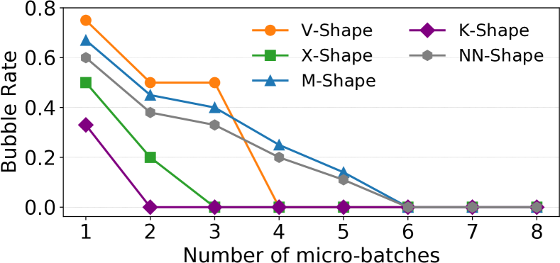
Figure 11: Bubble rate in terms of micro-batch numbers ($N_{R}$).

Bubble rate and $N_{R}$.   The bubble rate can be influenced by the number of micro-batches ($N_{R}$) involved in repetend construction. Figure 11 shows the bubble rate as $N_{R}$ increases for various operator placement strategies when the memory capacity is not constrained. Interestingly, we observed that all schedules can achieve a zero bubble rate when a sufficiently large number of micro-batches is used. However, it is worth noting that the starting number of micro-batches required to achieve a zero bubble rate differs across different operator placement strategies. For instance, the V-Shape placement requires a minimum of 4 micro-batches, which corresponds to the number of devices, while the NN-Shape and M-Shape placements requires at least 6 micro-batches. This suggests the necessity to search for a feasible number of micro-batches to achieve low device idle time.

Model	Parameters	Layer	Hidden Size	Head Number	Vocabulary Size
GPT [3]	{11B, 24B, 47B, 77B}	{32, 40, 48, 80}	{4096, 6144, 8192, 8192}	{32, 48, 64, 64}	{1M, 1M, 1M, 1.5M}
mT5 [43]	{1.8B, 9.5B, 43B, 88B}	{48, 48, 64, 80}	{1024, 3072, 6144, 8192}	{16, 24, 48, 64}	{512K, 1M, 1.5M, 1.5M}

TABLE III: Model architecture with increasing number of GPUs. K: thousand. M: million. B: billion.

Bubble rate and $M$.   To further investigate the impact of memory capacity ($M$) on the bubble rate, we conducted an ablation study by increasing memory capacity. In this study, we maintained the same starting $N_{R}$ that allowed us to achieve a zero bubble rate in Figure 11. For simplicity, we considered the memory consumption of each forward and backward block as 1 and -1, respectively. Figure 12 presents the bubble rate in relation to memory capacity. We observed that a lower memory capacity corresponds to a larger bubble rate. This is because it requires fewer forward execution blocks to be executed before the first backward execution block, thus filtering out schedules that could have executed them earlier for better device utilization. Similarly, as the memory capacity becomes sufficiently large, all schedules can ultimately achieve a zero bubble rate.

We noticed a strong correlation between $N_{R}$ and $M$ (Figures 11 and  12). We observed that the trend of the bubble rate tends to be similar when increasing $N_{R}$ and $M$. Intuitively, a larger $N_{R}$ exposes a broader space for scheduling, allowing more forward execution blocks to be executed ahead of time and thereby improving device utilization. Similar results are observed for higher memory capacity.

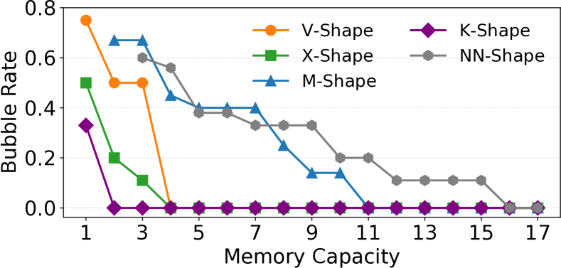
Figure 12: Bubble rate in terms of memory capacity ($M$).

VI-D End-to-end Runtime Performance

We evaluated the training performance of GPT and mT5, and the inference performance of Flava. For other scenarios, e.g., inference of GPT, Tessel demonstrates comparable performance to the baselines. We set the global size to 128 during training and tuned the micro-batch size to reach the best performance. Table III illustrates the model configurations used during the evaluation as we increased the number of GPUs. Similar to Alpa [45], we used aggregated Peta Floating-point Operations Per Second (PFLOPS) as the performance metric during training.

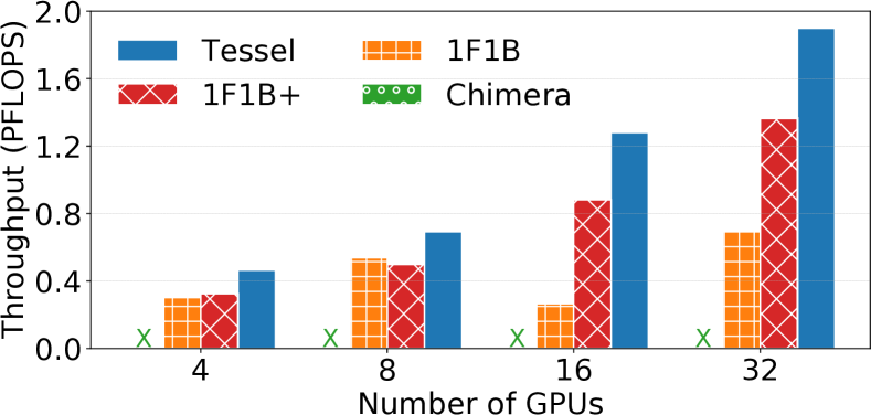
Figure 13: GPT end-to-end training throughput. ($\times$: failure due to out of memory)

GPT training results.   Figure 13 illustrates the performance comparison between Tessel and the baselines during GPT training. Tessel achieved up to 4.8$\times$ (16-GPU) and 1.4$\times$ speedup compared to 1F1B and 1F1B+, respectively. Chimera failed to run in this scenario due to out-of-memory issues caused by its placement strategy, which co-located parameters of multiple stages within a single GPU, exacerbating the memory bottleneck. In multi-server cases, 1F1B encountered out-of-memory issues, with intra-server tensor parallelism necessitating the application of cross-server tensor parallelism to distribute the large embedding layer. This lead to heavy communication overhead. 1F1B+ instead adopted the M-Shape placement strategy that only required the embedding layer to perform cross-server communication, improving performance by saving communication costs. However, 1F1B+ still suffered from inefficiency due to data dependency. Tessel adopted the same placement strategy as 1F1B+ and outperformed it by searching for a more efficient schedule.

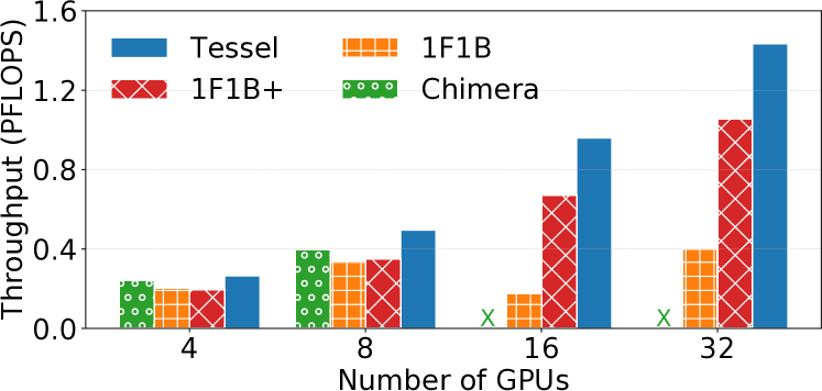
Figure 14: mT5 end-to-end training throughput. ($\times$: failure due to out of memory)

mT5 training results.   Figure 14 compares the performance of Tessel with the baselines on mT5 training. Overall, Tessel achieves up to 5.5$\times$ and 1.4$\times$ performance speedup compared to existing schedules and 1F1B+, respectively. Within one server, Chimera slightly outperformed 1F1B+, due to the lower bubble rate indicated in Table II. When scaled to multiple servers, 1F1B+ outperformed 1F1B for similar reasons as observed in the GPT results. Tessel still maintained its superior performance over all baselines by identifying the zero-bubble schedule for the advanced placement.

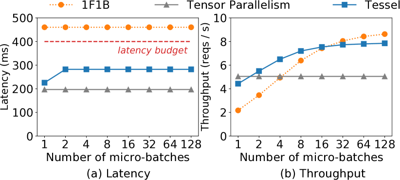
Figure 15: Inference latency and throughput of Flava (24 layers, 4096 hidden size with 32 heads) on 4 GPUs.

Flava inference results.   Inference workloads often come with latency budget requirements, with 400 ms being a recommended setting based on previous studies [41, 6]. While meeting the latency budget is crucial, service providers can further benefit from increasing throughput to save costs. Therefore, pipeline parallelism can be an effective choice to further enhance throughput while adhering to latency constraints. For the inference evaluation, we used the Flava model on 4 GPUs. Since there is no straightforward adaptation of 1F1B to the K-Shape, we solely compared the conventional 1F1B and tensor parallelism [30] with Tessel.

Figure 15 illustrates the latency-throughput trade-offs for various micro-batch sizes. Notably, 1F1B focuses on optimizing throughput, while tensor parallelism prioritizes latency. In contrast, Tessel demonstrates a more balanced trade-off by slightly increasing latency within the budget while significantly improving throughput, resulting in 1.5$\times$ throughput speedup compared to tensor parallelism. 1F1B demostrates high throughput only for large micro-batch sizes, but it falls short in optimizing latency, consistently failing to meet the latency budget. In Tessel with 1F1B, the latency speedup is attributed to the concurrent execution of independent branches on multiple devices, whereas 1F1B can only schedule the branches in sequential execution order. For a large number of micro-batches (e.g., 128), the throughput of Tessel is slightly lower than 1F1B due to kernel inefficiency when applying tensor parallelism on cross-encoder model parts. However, when the number of micro-batches is small, Tessel can achieve up to 2.0$\times$ throughput speedup over 1F1B. This boost is attributed to the lower latency of a single micro-batch execution, resulting in an overall shorter time to execute a small number of micro-batches. For tensor parallelism, 1F1B partitions operators into smaller ones that may not fully saturate the GPU during computation. In contrast, Tessel places independent branches on different devices without partitioning operators, preserving computation efficiency and improving throughput.

VI-E Runtime Performance Analysis

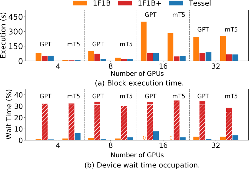
Figure 16: Runtime performance breakdown of (a) block execution time and (b) device wait occupation. The slashed region in (b) shows the theoretical estimation of wait time occupation.

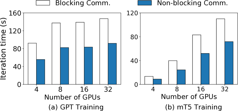
Figure 17: End-to-end training time of blocking and non-blocking communication of GPT (M-Shape) and mT5 (NN-Shape).

Performance breakdown.   Runtime execution can be divided into two components: block execution time and device waiting time. Device waiting time refers to the time span between the execution of neighboring blocks, including data communication between blocks and device idle time caused by data dependency. To accurately determine device waiting time in the schedules, we profiled the runtime at the slowest stage. Figure 16 displays (a) block execution time and (b) wait time occupation in relation to end-to-end training performance. Overall, wait time occupation remains below 6% overhead of the theoretical estimation (slashed region in Figure 16(b)), showcasing Tessel’s efficient runtime implementation. Both 1F1B and Tessel have theoretically zero bubble rate and achieve low device wait time occupation. However, Tessel outperforms 1F1B significantly due to its more balanced block execution workloads across devices. For instance, in GPT training with 16 GPUs, 1F1B requires almost 400 seconds for block computation on the slowest device, while Tessel only requires around 100 seconds. Comparing Tessel with 1F1B+, both employ the same placement strategy, resulting in similar block execution costs. However, Tessel outperforms 1F1B+ by searching for more efficient schedules that significantly reduce device wait time during runtime.

Non-blocking communication.   Tessel adopts non-blocking communication to overlap the communication with the computation, resulting in improved device utilization. In Figure 17(a) and (b), we show the end-to-end training performance comparison of Tessel with both blocking and non-blocking communication on GPT and mT5, respectively. By utilizing non-blocking communication, Tessel achieves up to 1.9$\times$ speedup. We do not show the performance of schedules that are based on V-Shape, X-Shape, and K-Shape, as their communication can occasionally happen at the same time between execution blocks, resulting in similar performance.

VII Related Work

Schedules.   Existing research has primarily focused on generally applicable efficient schedules. Notably, 1F1B [8, 21, 20] and GPipe [10] are popular schedules widely applied in practical settings. Many works have built upon 1F1B to further enhance efficiency by incorporating additional techniques [2, 46, 23]. For example, Varuna [2] considers schedules with recompute by eliminating recompute at the last pipeline stage. Some schedules also take memory constraints into account [11, 17]. For instance, Gems [11] proposes a memory-efficient schedule by considering two model replicas. These handcrafted schedules can also be searched automatically by using Tessel. Furthermore, Tessel can also accommodate the operator placements that are beyond the support of such predefined schedules.

Software pipeline optimizations.   In the domain of parallel computing, similar pipeline problems [1] revolve around efficiently parallelizing instructions within loop code. These optimizations also involve identifying efficient kernels (i.e., similar to repetend in Tessel) by conducting a thorough analysis of data dependencies among instructions and capitalizing on hardware capabilities [5, 28, 15, 32]. For example, URPR [32] unrolls the loop by several iterations and re-orders instructions to identify kernels. In the context of DNN execution, Tessel tackles a unique pipeline problem characterized by explicit data dependencies among blocks, variable computation cost of blocks and additional constraints such as memory capacity.

Parallelization techniques.   In addition to the schedules related to operator placement strategies, there are other parallelization [34, 12, 38, 30, 4, 27, 26, 9] techniques that can help improve performance. For example, tensor parallelism [12, 38, 30] enables the partitioning of a single operator across multiple devices for concurrent execution, and DeepSpeed [27] leverages ZeRO [26, 29] to offload tensors to CPU or other devices. These techniques are complementary to the schedule and can be viewed as operator placement for Tessel to generate corresponding schedules.

Automated parallelization.   The automation of distributed DNN training and inference is important for large and diverse models. Existing works [45, 33, 42] mainly consider combining tensor parallelism with pipeline parallelism and search for feasible configurations of each parallelism. For example, Alpa [45] uses an ILP solver for tensor parallelism and dynamic programming for pipeline parallelism. Works like theses are designed to adpot a predefined schedule like 1F1B. Complementing Tessel, these search algorithms can further extend their various operator placement strategies using Tessel’s schedule search for better performance.

VIII Conclusion

Tessel is an efficient and automated DNN schedule-searching system that can accommodate diverse operator placement strategies. Based on the observation of repetends in DNN schedules, Tessel greatly reduces the schedule search space while delivering high performance results. We believe that Tessel can help parallel DNN training and inference systems to better exploit their performance. More importantly, we hope that the DNN schedule properties that Tessel has revealed can inspire more relevant research in the future.

IX Acknowledgments

We thank all the anonymous reviewers for their insightful comments during the paper reviewing period. This work is supported in part by the National Natural Science Foundation of China under Grant No. 62141216, 62172382, and 61832011. Cheng Li and Youshan Miao are the corresponding authors.

References

- [1] V. H. Allan, R. B. Jones, R. M. Lee, and S. J. Allan, “Software pipelining,” ACM Computing Surveys (CSUR), 1995.
- [2] S. Athlur, N. Saran, M. Sivathanu, R. Ramjee, and N. Kwatra, “Varuna: scalable, low-cost training of massive deep learning models,” in Proceedings of the Seventeenth European Conference on Computer Systems, 2022, pp. 472–487.
- [3] T. Brown, B. Mann, N. Ryder, M. Subbiah, J. D. Kaplan, P. Dhariwal, A. Neelakantan, P. Shyam, G. Sastry, A. Askell et al., “Language models are few-shot learners,” Advances in neural information processing systems, 2020.
- [4] T. Chen, B. Xu, C. Zhang, and C. Guestrin, “Training deep nets with sublinear memory cost,” arXiv preprint arXiv:1604.06174, 2016.
- [5] W. Y. Chen, S. A. Mahlke, N. J. Warter, S. Anik, and W.-M. W. Hwu, “Profile-assisted instruction scheduling,” International Journal of Parallel Programming, 1994.
- [6] Y. Chen, T. Farley, and N. Ye, “Qos requirements of network applications on the internet,” Information Knowledge Systems Management, 2004.
- [7] L. De Moura and N. Bjørner, “Z3: An efficient smt solver,” in Tools and Algorithms for the Construction and Analysis of Systems: 14th International Conference (TACAS 2008). Springer, 2008, pp. 337–340.
- [8] S. Fan, Y. Rong, C. Meng, Z. Cao, S. Wang, Z. Zheng, C. Wu, G. Long, J. Yang, L. Xia et al., “Dapple: A pipelined data parallel approach for training large models,” in Proceedings of the 26th ACM SIGPLAN Symposium on Principles and Practice of Parallel Programming, 2021, pp. 431–445.
- [9] C.-C. Huang, G. Jin, and J. Li, “Swapadvisor: Pushing deep learning beyond the gpu memory limit via smart swapping,” in Proceedings of the Twenty-Fifth International Conference on Architectural Support for Programming Languages and Operating Systems, 2020, pp. 1341–1355.
- [10] Y. Huang, Y. Cheng, A. Bapna, O. Firat, D. Chen, M. Chen, H. Lee, J. Ngiam, Q. V. Le, Y. Wu et al., “Gpipe: Efficient training of giant neural networks using pipeline parallelism,” in Advances in Neural Information Processing Systems, 2019, pp. 103–112.
- [11] A. Jain, A. A. Awan, A. M. Aljuhani, J. M. Hashmi, Q. G. Anthony, H. Subramoni, D. K. Panda, R. Machiraju, and A. Parwani, “Gems: Gpu-enabled memory-aware model-parallelism system for distributed dnn training,” in SC20: International Conference for High Performance Computing, Networking, Storage and Analysis. IEEE, 2020, pp. 1–15.
- [12] Z. Jia, M. Zaharia, and A. Aiken, “Beyond data and model parallelism for deep neural networks,” SysML 2019, 2019.
- [13] A. B. Kahn, “Topological sorting of large networks,” Communications of the ACM, 1962.
- [14] W. Kim, B. Son, and I. Kim, “Vilt: Vision-and-language transformer without convolution or region supervision,” in International Conference on Machine Learning, 2021, pp. 5583–5594.
- [15] Y. Kim, J. Lee, T. X. Mai, and Y. Paek, “Improving performance of nested loops on reconfigurable array processors,” ACM Transactions on Architecture and Code Optimization (TACO), 2012.
- [16] V. A. Korthikanti, J. Casper, S. Lym, L. McAfee, M. Andersch, M. Shoeybi, and B. Catanzaro, “Reducing activation recomputation in large transformer models,” Proceedings of Machine Learning and Systems, 2023.
- [17] S. Li and T. Hoefler, “Chimera: efficiently training large-scale neural networks with bidirectional pipelines,” in Proceedings of the International Conference for High Performance Computing, Networking, Storage and Analysis, 2021, pp. 1–14.
- [18] Z. Lin, Y. Miao, G. Liu, X. Shi, Q. Zhang, F. Yang, S. Maleki, Y. Zhu, X. Cao, C. Li et al., “Superscaler: Supporting flexible dnn parallelization via a unified abstraction,” arXiv preprint arXiv:2301.08984, 2023.
- [19] Z. Liu, H. Hu, Y. Lin, Z. Yao, Z. Xie, Y. Wei, J. Ning, Y. Cao, Z. Zhang, L. Dong et al., “Swin transformer v2: Scaling up capacity and resolution,” in Proceedings of the IEEE/CVF conference on computer vision and pattern recognition, 2022, pp. 12 009–12 019.
- [20] D. Narayanan, A. Harlap, A. Phanishayee, V. Seshadri, N. R. Devanur, G. R. Ganger, P. B. Gibbons, and M. Zaharia, “Pipedream: generalized pipeline parallelism for dnn training,” in Proceedings of the 27th ACM Symposium on Operating Systems Principles, 2019, pp. 1–15.
- [21] D. Narayanan, M. Shoeybi, J. Casper, P. LeGresley, M. Patwary, V. Korthikanti, D. Vainbrand, P. Kashinkunti, J. Bernauer, B. Catanzaro et al., “Efficient large-scale language model training on gpu clusters using megatron-lm,” in Proceedings of the International Conference for High Performance Computing, Networking, Storage and Analysis, 2021, pp. 1–15.
- [22] OpenAI, “GPT-4 Introduction,” https://openai.com/product/gpt-4, [Online; accessed May-2023.
- [23] J. H. Park, G. Yun, M. Y. Chang, N. T. Nguyen, S. Lee, J. Choi, S. H. Noh, and Y.-r. Choi, “Hetpipe: Enabling large dnn training on (whimpy) heterogeneous gpu clusters through integration of pipelined model parallelism and data parallelism,” in 2020 USENIX Annual Technical Conference (USENIX ATC 20), 2020, pp. 307–321.
- [24] PyTorch Team, “PyTorch,” https://pytorch.org//, [Online; accessed Mar.-2022.
- [25] A. Radford, K. Narasimhan, T. Salimans, and I. Sutskever, “Improving language understanding by generative pre-training,” arXiv preprint arXiv:1704.01444, 2018.
- [26] S. Rajbhandari, J. Rasley, O. Ruwase, and Y. He, “Zero: Memory optimizations toward training trillion parameter models,” in SC20: International Conference for High Performance Computing, Networking, Storage and Analysis. IEEE, 2020, pp. 1–16.
- [27] J. Rasley, S. Rajbhandari, O. Ruwase, and Y. He, “Deepspeed: System optimizations enable training deep learning models with over 100 billion parameters,” in Proceedings of the 26th ACM SIGKDD International Conference on Knowledge Discovery & Data Mining, 2020, pp. 3505–3506.
- [28] B. R. Rau, M. Lee, P. P. Tirumalai, and M. S. Schlansker, “Register allocation for software pipelined loops,” in Proceedings of the ACM SIGPLAN 1992 conference on Programming language design and implementation, 1992, pp. 283–299.
- [29] J. Ren, S. Rajbhandari, R. Y. Aminabadi, O. Ruwase, S. Yang, M. Zhang, D. Li, and Y. He, “Zero-offload: Democratizing billion-scale model training,” in 2021 USENIX Annual Technical Conference (USENIX ATC 21), 2021, pp. 551–564.
- [30] M. Shoeybi, M. Patwary, R. Puri, P. LeGresley, J. Casper, and B. Catanzaro, “Megatron-lm: Training multi-billion parameter language models using gpu model parallelism,” arXiv preprint arXiv:1909.08053, 2019.
- [31] A. Singh, R. Hu, V. Goswami, G. Couairon, W. Galuba, M. Rohrbach, and D. Kiela, “Flava: A foundational language and vision alignment model,” in Proceedings of the IEEE/CVF Conference on Computer Vision and Pattern Recognition, 2022, pp. 15 638–15 650.
- [32] B. Su, S. Ding, and J. Xia, “Urpr—an extension of urcr for software pipelining,” in Proceedings of the 19th annual workshop on Microprogramming, 1986, pp. 94–103.
- [33] J. M. Tarnawski, D. Narayanan, and A. Phanishayee, “Piper: Multidimensional planner for dnn parallelization,” Advances in Neural Information Processing Systems, 2021.
- [34] P. Team, “Distributed Data Parallelism,” https://pytorch.org/docs/stable/notes/ddp.html, [Online; accessed Sep.-2022.
- [35] P. Team, “TorchScript,” https://pytorch.org/docs/stable/jit.html.
- [36] A. Vaswani, N. Shazeer, N. Parmar, J. Uszkoreit, L. Jones, A. N. Gomez, Ł. Kaiser, and I. Polosukhin, “Attention is all you need,” Advances in neural information processing systems, 2017.
- [37] G. Wang, X. Fang, Z. Wu, Y. Liu, Y. Xue, Y. Xiang, D. Yu, F. Wang, and Y. Ma, “Helixfold: An efficient implementation of alphafold2 using paddlepaddle,” arXiv preprint arXiv:2207.05477, 2022.
- [38] M. Wang, C.-c. Huang, and J. Li, “Supporting very large models using automatic dataflow graph partitioning,” in Proceedings of the Fourteenth EuroSys Conference 2019, 2019, pp. 1–17.
- [39] Z. Wang, J. Yu, A. W. Yu, Z. Dai, Y. Tsvetkov, and Y. Cao, “Simvlm: Simple visual language model pretraining with weak supervision,” arXiv preprint arXiv:2108.10904, 2021.
- [40] G. J. Woeginger, “Exact algorithms for np-hard problems: A survey,” in Combinatorial Optimization—Eureka, You Shrink!, 2003, pp. 185–207.
- [41] X. Xiao, Technical, commercial and regulatory challenges of QoS: An internet service model perspective. Morgan Kaufmann, 2008.
- [42] Y. Xu, H. Lee, D. Chen, B. Hechtman, Y. Huang, R. Joshi, M. Krikun, D. Lepikhin, A. Ly, M. Maggioni et al., “Gspmd: General and scalable parallelization for ml computation graphs,” arXiv preprint arXiv:2105.04663, 2021.
- [43] L. Xue, N. Constant, A. Roberts, M. Kale, R. Al-Rfou, A. Siddhant, A. Barua, and C. Raffel, “mt5: A massively multilingual pre-trained text-to-text transformer,” arXiv preprint arXiv:2010.11934, 2020.
- [44] B. Zheng, L. Dong, S. Huang, S. Singhal, W. Che, T. Liu, X. Song, and F. Wei, “Allocating large vocabulary capacity for cross-lingual language model pre-training,” in Empirical Methods in Natural Language Processing, 2021, pp. 3203––3215.
- [45] L. Zheng, Z. Li, H. Zhang, Y. Zhuang, Z. Chen, Y. Huang, Y. Wang, Y. Xu, D. Zhuo, E. P. Xing et al., “Alpa: Automating inter-and Intra-Operator parallelism for distributed deep learning,” in 16th USENIX Symposium on Operating Systems Design and Implementation (OSDI 22), 2022, pp. 559–578.
- [46] Y. Zhuang, L. Zheng, Z. Li, E. Xing, Q. Ho, J. Gonzalez, I. Stoica, H. Zhang, and H. Zhao, “On optimizing the communication of model parallelism,” Proceedings of Machine Learning and Systems, 2023.