Tomographic cross-correlations between galaxy surveys and CMB gravitational lensing potential – impact of redshift bin mismatch

Abstract

Context. Upcoming surveys of the large scale structure will employ large coverage area around half of the sky, and a significant increase in the depth of observations. With these surveys we will be able to perform cross-correlations between CMB gravitational lensing and galaxy surveys divided into narrow redshift bins to map the evolution of the cosmological parameters with redshift.

Aims. To study the impact of redshift bin mismatch of objects due to photometric redshift errors on tomographic cross-correlation measurements.

Methods. We use the FLASK code to create Monte Carlo simulations of the LSST galaxy survey and Planck CMB lensing convergence. We simulate log-normal fields and divide galaxies into $9$ redshift bins, with Gaussian photometric redshift errors. To estimate parameters, we use angular power spectra of CMB lensing and galaxy density contrast fields and the Maximum Likelihood Estimation method.

Results. We show that even with the simple Gaussian errors with standard deviation of $\sigma(z)=0.02(1+z)$, the galaxy auto-power spectra in tomographic bins suffer offsets varying between $2-15\%$. The estimated cross-power spectra between galaxy clustering and CMB lensing are also biased with smaller deviations $<5\%$. The $\sigma_{8}$ parameter, as a result, shows deviations between $0.2-1.2\,\sigma$ due to redshift bin mismatch of objects. We propose a computationally fast and robust method based on the scattering matrix approach (Zhang et al., 2010) to correct for the redshift bin mismatch of objects.

Conclusions. The estimation of parameters in tomographic studies like galaxy linear bias, amplitude of cross-correlation, and $\sigma_{8}$ are biased due to redshift bin mismatch of objects. The biases in these parameters get alleviated with our scattering matrix approach.

1 Introduction

The large-scale structure in the Universe has been a key contributor to testing the theories of gravity, the nature of dark energy and dark matter. It gives us vital information about the growth of structure in the Universe and cosmic expansion history. Observations from the galaxy survey experiments like Sloan Digital Sky Survey (SDSS, Gunn et al. 2006; Strauss et al. 2002), Wide-field Infrared Survey Explorer (WISE, Schlafly et al. 2019; Wright et al. 2010), Kilo-Degree Survey (KiDS, Heymans et al. 2021; de Jong et al. 2015), Hyper Suprime-Cam (HSC, Hikage et al. 2019), Two Micron All Sky Survey (2MASS, Bilicki et al. 2014), and Dark Energy Survey (DES, Abbott et al. 2018) have been the torch-bearer in unveiling the shortcomings of the standard model of cosmology, the $\Lambda$CDM model. The baton is now with the upcoming galaxy surveys including the Vera C. Rubin Observatory Legacy Survey of Space and Time (LSST, Ivezić et al. 2019; LSST Science Collaboration et al. 2009), Euclid (Laureijs et al., 2011), Nancy Grace Roman Space Telescope (Spergel et al., 2013), Dark Energy Spectroscopic Instrument (DESI, Dey et al. 2019), and Spectro-Photometer for the History of the Universe, Epoch of Reionization, and Ices Explorer (SPHEREx, Doré et al. 2014) to provide an in-depth understanding of the workings of our Universe.

The Cosmic Microwave Background (CMB) gives a view of the infant Universe and carries information about the energy components of the Universe. The gravitational lensing of the CMB carries information about the growth of structure at redshift $1-3$. The CMB lensing signal has been valuable in studying the properties of dark energy and is a complementary probe to galaxy clustering and galaxy weak lensing. Cross-correlations between the lensing map of CMB and tracers of large-scale structure can be used to extract information about the evolution of the large-scale gravitational potential. The importance of cross-correlations between CMB lensing convergence and galaxy positions in testing the validity of the $\Lambda$CDM model has been firmly established with many studies performed over the past years (Saraf et al. 2022; Miyatake et al. 2022; Robertson et al. 2021; Krolewski et al. 2021; Darwish et al. 2021 Abbott et al. 2019; Bianchini & Reichardt 2018; Singh et al. 2017; Bianchini et al. 2016; Bianchini et al. 2015).

Cross-correlation tomography performed with galaxy samples divided into narrow redshift bins also allows us to map the evolution of the cosmological parameters with redshift. Several tomographic cross-correlation studies (such as Wang et al. 2023; Yu et al. 2022; White et al. 2022; Pandey et al. 2022; Chang et al. 2022; Sun et al. 2022; Krolewski et al. 2021; Hang et al. 2021; Marques & Bernui 2020; Peacock & Bilicki 2018; Giannantonio et al. 2016) have identified differences in the value of cosmological parameters like the $\sigma_{8}$, $\Omega_{m}$, or the combined $S_{8}$ parameter (defined as $S_{8}\equiv\sigma_{8}\sqrt{\Omega_{m}/0.3}$) within the $\Lambda$CDM model. These low-redshift cross-correlation probes consistently measure a lower value for these parameters as compared to the high-redshift only-CMB measurements from Planck satellite (Planck Collaboration et al., 2020a), resulting in the so-called $S_{8}$ and $\sigma_{8}-\Omega_{m}$ tensions. Other studies like Bianchini & Reichardt (2018), Amon et al. (2018), Blake et al. (2016), Giannantonio et al. (2016) and Pullen et al. (2016) find consistent deviations in the values of $D_{g}$ and $E_{g}$ statistics when testing the $\Lambda$CDM model with different galaxy surveys. The galaxy survey experiments in the future will play a pivotal role in increasing the significance of either tension or agreement in cosmological parameters and quantifying possible deviations from the standard $\Lambda$CDM model.

In this paper, we present a tomographic cross-correlation study through $300$ Monte Carlo (MC) simulations of the Vera C. Rubin Observatory Legacy Survey of Space and Time (LSST) galaxy survey and Planck CMB lensing convergence. We include root mean square scatter in redshifts $\frac{\sigma(z)}{1+z}=0.02\text{ and }0.05$ but exclude catastrophic redshift errors and photometric calibrations errors from our simulations, thus superficially creating the best possible observations. We show that even for such idealistic observations the photometric redshift uncertainties in the redshift distributions produce biased estimates of cross-correlation if redshift bin mismatch of objects due to photometric redshift errors are not properly taken into account. Although few attempts have been made to account for this effect (Balaguera-Antolínez et al. 2018; Hang et al. 2021), we propose new fast and efficient method of unbiased estimation of tomographic cross-correlation using the scattering matrix formalism introduced by Zhang et al. (2010).

The paper is organised as follows: section 2 presents the simulation setup and the theoretical background, section 3 describes the methodology to compute the power spectra, reconstruct true redshift distributions and estimate parameters. In section 4, we present the validation results of our simulations and estimation of galaxy auto-power spectra and cross-power spectra between galaxy over-density and CMB lensing convergence. We discuss the correction to the power spectra through the scattering matrix in section 5 and quantify the impact on galaxy linear bias and amplitude of cross-correlation parameters in section 6. We study the apparent tension on the $\sigma_{8}$ parameter due to redshift bin mismatch in section 7. Finally, we summarise our results in section 8.

2 Simulations and Theory

We use the publicly available code FLASK (Xavier et al., 2016) to generate 300 tomographic MC realisations of correlated lognormal galaxy over-density and CMB lensing convergence fields. The galaxy density follows LSST photometric redshift distribution profile (Ivezić et al. 2019; LSST Science Collaboration et al. 2009) with mean redshift $0.9$ and mean surface number density of $40\text{ arcmin}^{-2}$. The simulated CMB lensing convergence field is consistent with Planck observations (Planck Collaboration et al., 2020b). The galaxy density field is induced with Poisson noise, and for CMB convergence we use the noise power spectrum provided in the Planck 2018 data package. Due to limitations of computational capabilities, the sky area covered in our simulations is $2000\text{ deg}^{2}$. However, the results obtained in this study should remain valid for the planned area of the LSST survey, provided the errors are appropriately scaled by the fraction of sky coverage. The mock galaxy samples are divided into $9$ disjoint tomographic bins with redshift intervals $(0.0,0,2,0.4,0.6,0.8,1.0,1.4,1.8,2.2,3.0]$, as marked by the dashed vertical lines in Fig. 1.

The fiducial angular power spectra for each redshift bin used to generate correlated maps are computed under the Limber approximation (Limber, 1953) using

$$C_{\ell}^{xy}=\int\limits_{0}^{\infty}\frac{\mathrm{d}z}{c}\frac{H(z)}{\chi^{2}(z)}W^{x}(z)W^{y}(z)P\bigg{(}k=\frac{\ell+1/2}{\chi(z)},z\bigg{)}$$ (1)

where $\{x,y\}\in\{\kappa,g\}$, $\kappa\equiv$ convergence and $g\equiv$ galaxy over-density, $c$ is the speed of light, and $P(k,z)$ is the matter power spectrum generated using the public software CAMB (Lewis et al., 2000) using the HALOFIT prescription. The kernels $W^{x}(z)$ connects the observables to the underlying total matter distribution. Assuming a flat Universe (Planck Collaboration et al., 2020a), the lensing kernel $W^{\kappa}(z)$ and the galaxy kernel $W^{g}(z)$ are expressed as

$$W^{\kappa}(z) =\frac{3\Omega_{m}}{2c}\frac{H_{0}^{2}}{H(z)}(1+z)\chi(z)\frac{\chi_{*}-\chi(z)}{\chi_{*}}$$ (2)

$$W^{g}(z) =b(z)\frac{\mathrm{d}N}{\mathrm{d}z}$$ (3)

Here, $H(z)$ is the Hubble parameter at redshift $z$, $\chi(z)$ and $\chi_{*}$ are the comoving distances to redshift $z$ and the surface of last scattering. $\Omega_{m}$ and $H_{0}$ are the present-day values of the matter density parameter and Hubble constant, respectively. $\frac{\mathrm{d}N}{\mathrm{d}z}$ stands for the normalised redshift distribution of galaxies, and $b(z)$ is the linear galaxy bias that relates the galaxy over-density to the total underlying matter density (Fry & Gaztanaga, 1993). We assume in this study that there is no contribution to the galaxy kernel from magnification bias, leaving study of its impact for future work. The expressions for kernels $W^{\kappa}(z)$ and $W^{g}(z)$ given by Eqs. (2-3) is valid in flat Universe model (i.e., for zero curavture).

We use a redshift dependent model of galaxy bias (Solarz et al. 2015; Moscardini et al. 1998; Fry 1996):

$$b(z)=1+\frac{b_{0}-1}{D(z)}$$ (4)

where we take $b_{0}\equiv b(z=0)=1.3$ and $D(z)$ is the linear growth function normalised to unity at $z=0$

$$D(z)=\exp\bigg{\{}-\int\limits_{0}^{z}\frac{[\Omega_{m}(z^{\prime})]^{\gamma}}{1+z^{\prime}}\mathrm{d}z^{\prime}\bigg{\}}$$ (5)

where $\gamma=0.55$ is the growth index for the General Relativity (Linder, 2005).

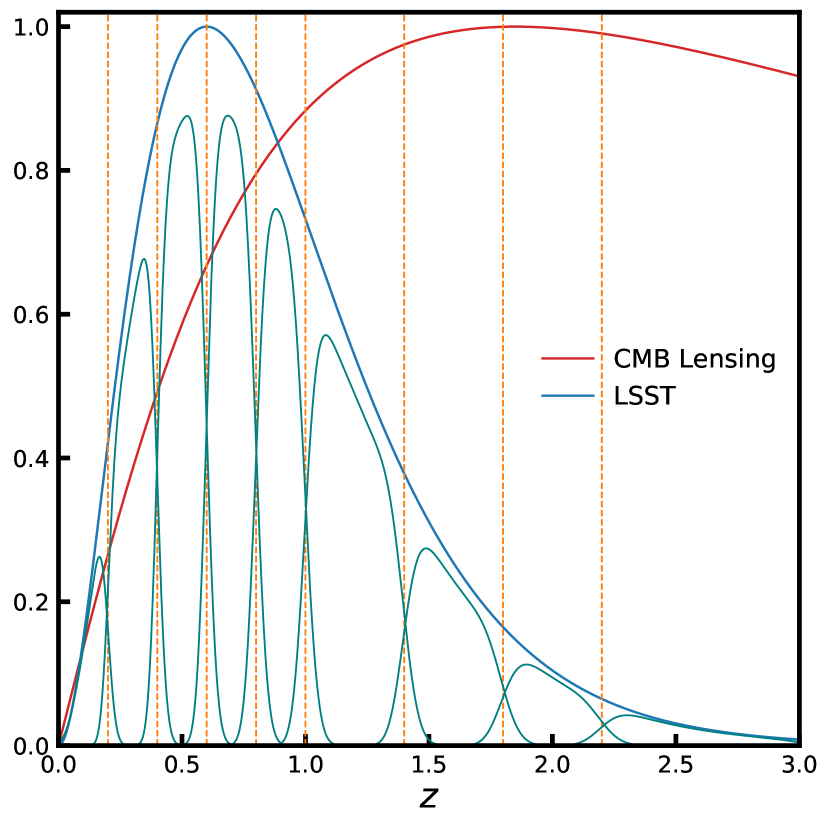
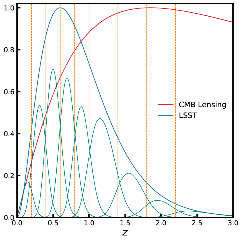
Figure 1: True LSST redshift distribution (blue solid curve) divided into 9 photometric redshift bins (shown by solid green curves) for $\sigma_{0}=0.02$ (left) and $\sigma_{0}=0.05$ (right). The red line denotes the CMB lensing kernel and the orange dashed vertical lines mark the true redshift bins. The full LSST redshift distribution and CMB lensing kernel are normalized to unit maximum.

For every simulation, the FLASK code produces CMB convergence map and galaxy number count maps for each tomographic bin along with the catalogue of galaxy redshifts. We term these maps as true datasets. We generate photometric redshifts, $z_{p}$, for galaxies in every simulation by drawing positive random values from Gaussian distributions with their true redshift $z_{t}$ as the mean and standard deviation $\sigma_{0}(1+z_{t})$. We adopt two different values of $\sigma_{0}$: $0.02\text{ and }0.05$, to study the dependence of our results on the strength of redshift scatters. The galaxies are again divided into $9$ tomographic bins based on their photometric redshifts. In Fig. 1, we show the true LSST redshift distribution (blue solid curve) divided into $9$ photometric redshift bins (solid green lines) and the CMB lensing kernel (red solid curve) in the redshift range $0\leq z\leq 3$. The green lines represent how the disjoint true redshift bins transform after introducing the photometric redshift errors. The orange dashed vertical lines mark the boundaries of true redshift bins.

We build galaxy over-density maps from photometric number count maps (hereafter, photometric datasets) with HEALPix (Górski et al., 2005) resolution parameter $N_{\text{side}}=1024$ using

$$g(\hat{\textbf{n}})=\frac{n(\hat{\textbf{n}})-\overline{n}}{\overline{n}}$$ (6)

where $n(\hat{\textbf{n}})$ is the number of galaxies at angular position $\hat{\textbf{n}}$ and $\overline{n}$ is the mean number of galaxies per pixel. In Table 1, we present from one realisation the comparison of the mean number of objects per pixel (for $N_{\text{side}}=1024$) and median redshift between true and photometric datasets.

For the simulations and analyses presented in this paper, we adopt the flat $\Lambda$CDM cosmology with best-fit Planck + WP + highL + lensing cosmological parameters, as described in Planck Collaboration et al. (2020a). Here, WP refers to WMAP polarisation data at low multipoles, highL is the high-resolution CMB data from Atacama Cosmology Telescope (ACT), and South Pole Telescope (SPT) and lensing refer to the inclusion of Planck CMB lensing data in the parameter likelihood.

Table 1: Comparison of physical properties between true and photometric datasets for all tomographic bins from a single realization. $\overline{n}$ is the mean number of objects per pixel and $\overline{z}$ represents the median redshift of the tomographic bin.

$z$	$\overline{n}$ (true)	$\overline{n}$ (photo)		$\overline{z}$ (true)	$\overline{z}$ (photo)
		$\sigma_{0}=0.02$	$\sigma_{0}=0.05$		$\sigma_{0}=0.02$	$\sigma_{0}=0.05$
$[0.0,0.2)$	14.35	14.77	17.02	0.144	0.144	0.145
$[0.2,0.4)$	57.02	57.04	57.11	0.311	0.312	0.315
$[0.4,0.6)$	81.78	81.60	80.68	0.502	0.503	0.506
$[0.6,0.8)$	82.79	82.58	81.54	0.698	0.699	0.702
$[0.8,1.0)$	70.58	70.42	69.63	0.896	0.898	0.900
$[1.0,1.4)$	93.31	93.19	92.60	1.178	1.180	1.183
$[1.4,1.8)$	44.37	44.40	44.57	1.572	1.575	1.577
$[1.8,2.2)$	18.44	18.50	18.83	1.968	1.972	1.974
$[2.2,3.0)$	9.58	9.68	10.22	2.472	2.471	2.471

3 Methodology

In this section, we outline the method for computing power spectra from maps and estimating the true redshift distribution from photometric redshift distribution.

3.1 Estimation of power spectra

We extract the full sky power spectra from partial sky power spectra for every tomographic bin using a pseudo-$C_{\ell}$ method based on MASTER algorithm (Hivon et al., 2002), taking into account mode coupling induced by incomplete sky coverage and pixelization effects. We estimate the full sky power spectra in linearly spaced multipole bins with $\Delta\ell=30$ between $50\leq\ell\leq 1500$. The noise subtracted mean full sky power spectrum over $\text{N}_{\text{sim}}$ realisations is computed as (Saraf et al., 2022)

$$\overline{C}_{L}^{xy}\equiv\langle\hat{C}_{L}^{xy}\rangle=\frac{1}{\text{N}_{\text{sim}}}\sum_{i=1}^{\text{N}_{\text{sim}}}\hat{C}_{L}^{xy,i}-\langle{N}_{L}^{xy}\rangle_{\text{MC}}$$ (7)

where $\hat{C}_{L}^{xy,i}$ represents the full sky power spectrum estimate for $i^{\text{th}}$ simulation and $\langle{N}_{L}^{xy}\rangle_{\text{MC}}$ is the average noise power spectrum from Monte Carlo simulations. The errors associated with the mean power spectrum are computed from the diagonal of the power spectrum covariance matrix $\text{Cov}_{LL^{\prime}}^{xy}$ as

$$\Delta\overline{C}_{L}^{xy}=\bigg{(}\frac{\text{Cov}_{LL}^{xy}}{\text{N}_{\text{sim}}}\bigg{)}^{1/2}$$ (8)

where

$$\text{Cov}_{LL^{\prime}}^{xy}=\frac{1}{\text{N}_{\text{sim}}-1}\sum_{i=1}^{M}(\hat{C}_{L}^{xy,i}-\overline{C}_{L}^{xy})(\hat{C}_{L^{\prime}}^{xy,i}-\overline{C}_{L^{\prime}}^{xy})$$ (9)

3.2 Estimation of true redshift distribution

The true redshift distribution $\frac{\mathrm{d}N(z_{t})}{\mathrm{d}z_{t}}$ is estimated from the observed photometric redshift distribution $\frac{\mathrm{d}N(z_{p})}{\mathrm{d}z_{p}}$ and some quantification of errors on the photometric redshifts (from cross-validation with some spectroscopic survey or posteriors from machine learning methods). Often these errors are expressed by conditional probabilities $p(z_{p}-z_{t}|z_{t})$ and $p(z_{t}-z_{p}|z_{p})$ which we call photometric redshift error distributions. The true and photometric redshift distributions are then related through (Sheth & Rossi, 2010)

$$\frac{\mathrm{d}N(z_{t},z_{p})}{\mathrm{d}z_{t}\mathrm{d}z_{p}}=\frac{\mathrm{d}N(z_{t})}{\mathrm{d}z_{t}}p(z_{p}-z_{t}|z_{t})=\frac{\mathrm{d}N(z_{p})}{\mathrm{d}z_{p}}p(z_{t}-z_{p}|z_{p})$$ (10)

Thus depending on whether we have estimates of $p(z_{p}-z_{t}|z_{t})$ or $p(z_{t}-z_{p}|z_{p})$, the method for estimation of the true redshift distribution is called deconvolution or convolution, respectively.

3.2.1 Convolution method

When $p(z_{t}-z_{p}|z_{p})$ is known, we can estimate $\frac{\mathrm{d}N(z_{t})}{\mathrm{d}z_{t}}$ for each tomographic bin $i$ using convolution

$$\frac{\mathrm{d}N^{i}(z_{t})}{\mathrm{d}z_{t}}=\int\mathrm{d}z_{p}\frac{\mathrm{d}N^{i}(z_{p})}{\mathrm{d}z_{p}}p^{i}(z_{t}-z_{p}|z_{p})$$ (11)

where $\frac{\mathrm{d}N^{i}(z_{p})}{\mathrm{d}z_{p}}$ is the photometric redshift distribution of objects for the $i^{\text{th}}$ redshift bin. Generally, $p^{i}(z_{t}-z_{p}|z_{p})$ is fitted with parametric functions like Gaussian with assumed zero mean (Sun et al. 2022; Marques & Bernui 2020) or modified Lorentzian (Hang et al. 2021; Peacock & Bilicki 2018). Sheth & Rossi (2010) have shown that the quantity $p(z_{t}-z_{p}|z_{p})$ will be biased and not centered on zero. In our study, we fit the error distribution with a sum of three Gaussians

$$\mathcal{N}(x)=\sum\limits_{i=1}^{3}A_{i}\exp\bigg{[}\frac{(x-\mu_{i})^{2}}{2\sigma_{i}^{2}}\bigg{]}$$ (12)

where $A,\mu,\sigma$ control the amplitude, mean and width of the individual Gaussians. The sum of Gaussians can account for the bias in $p(z_{t}-z_{p}|z_{p})$, as well as other characteristic features of the error distributions like non-Gaussian wings and higher peak in the center. We also checked the fit with a higher number of Gaussians but did not find any improvement in the quality of fit beyond three Gaussians. For each of the tomographic bins, we fit for $A_{i},\mu_{i},\sigma_{i}$, and estimate the true redshift distribution using Eq. (11).

3.2.2 Deconvolution method

The true redshift distribution $\frac{\mathrm{d}N(z_{t})}{\mathrm{d}z_{t}}$ can be estimated by a deconvolution method when $p(z_{p}-z_{t}|z_{t})$ is known:

$$\frac{\mathrm{d}N(z_{p})}{\mathrm{d}z_{p}}=\int\mathrm{d}z_{t}\frac{\mathrm{d}N(z_{t})}{\mathrm{d}z_{t}}p(z_{p}-z_{t}|z_{t})$$ (13)

We fit $p(z_{p}-z_{t}|z_{t})$ with a single Gaussian and find the mean to be consistent with zero, in agreement with the unbiased nature of $p(z_{p}-z_{t}|z_{t})$ (Sheth & Rossi, 2010). We also fit the error distribution with a sum of Gaussians to find no significant improvement in the fit quality. Padmanabhan et al. (2005) proposed a deconvolution method based on Tikhonov regularisation, which lacks a general method to quantify the impact of penalty function on the reconstruction of $\frac{\mathrm{d}N(z_{t})}{\mathrm{d}z_{t}}$. We use a different approach to deconvolution. It is based on the convolution theorem and kernel-based regularisation (Meister, 2009). The true redshift distribution in our approach is estimated as

$$\frac{\mathrm{d}N(z_{t})}{\mathrm{d}z_{t}}=\mathcal{F}^{-1}\bigg{[}\frac{\mathcal{F}[\frac{\mathrm{d}N(z_{p})}{\mathrm{d}z_{p}}]}{\mathcal{F}[p(z_{p}-z_{t}|z_{t})]}\bigg{]}$$ (14)

where $\mathcal{F}$ and $\mathcal{F}^{-1}$ represent the Fourier and inverse Fourier transforms, respectively. We show the performance of our deconvolution method through a toy example in Appendix A.

We estimate the true redshift distribution for the entire redshift range, $0<z\leq 3$. Then, the true redshift distribution for each tomographic bin, $i$, can be expressed as

$$\frac{\mathrm{d}N^{i}}{\mathrm{d}z_{t}}=\frac{\mathrm{d}N}{\mathrm{d}z_{t}}W^{i}(z_{t})$$ (15)

where $W^{i}(z_{t})$ is a window function defining $i^{\text{th}}$ bin for true redshifts given by a step function:

$$W^{i}(z_{t})=\begin{cases}1,&\text{if}\quad z^{i}_{\text{min}}\leq z_{t}<z^{i+1}_{\text{min}}\\ 0,&\text{otherwise}\end{cases}$$ (16)

The corresponding photometric redshift distribution for every tomographic bin $i$ is given by

$$\frac{\mathrm{d}N^{i}(z_{p})}{\mathrm{d}z_{p}}=\int\mathrm{d}z_{t}\frac{\mathrm{d}N^{i}(z_{t})}{\mathrm{d}z_{t}}p^{i}(z_{p}-z_{t}|z_{t})$$ (17)

where $p^{i}(z_{p}-z_{t}|z_{t})$ is the error distribution for bin $i$. Eq. (13) will not follow convolution strictly near $z=0$, since negative redshifts are unphysical. Due to this fact, the reconstructed true redshift distribution will be inaccurate close to redshift $z=0$, and we expect these inaccuracies to affect to some extent the first two tomographic bins.

3.3 Galaxy bias and cross-correlation amplitude

For every tomographic bin, we estimate two parameters: galaxy linear bias $b$ and amplitude of the cross-power spectrum $A$. We assume the galaxy linear bias to be constant in each tomographic bin. It is a fairly good assumption for redshift bins which are narrow relative to the redshift dependence of the bias. The amplitude of the cross-power spectrum acts as a re-scaling of the observed cross-power spectrum to the fiducial theoretical power spectrum. From an unbiased estimation of the cross-power spectrum, we expect $A=1$ in the $\Lambda$CDM cosmology.

The galaxy auto-power spectrum scales as $b^{2}$, while the cross-power spectrum depends on the product $b\times A$. To break this degeneracy, we perform Maximum Likelihood Estimation on the joint data vector $\hat{C}_{L}=(\hat{C}_{L}^{\kappa g},\hat{C}_{L}^{gg})$, using the likelihood function

$$\begin{split}\mathcal{L}&(\hat{C}_{L}|b,A)=\frac{1}{\sqrt{(2\pi)^{N_{L}}det(\text{Cov}_{LL^{\prime}})}}\times\\ &\times\text{exp}\bigg{\{}-\frac{1}{2}[\hat{C}_{L}-C_{L}(b,A)](\text{Cov}_{LL^{\prime}})^{-1}[\hat{C}_{L^{\prime}}-C_{L^{\prime}}(b,A)]\bigg{\}}\end{split}$$ (18)

where $C_{L}(b,A)$ is the joint theoretical power spectrum template defined as $C_{L}(b,A)=(AC_{L}^{\kappa g}(b),C_{L}^{gg}(b))$, and the covariance matrix is given as

$$\text{Cov}_{LL^{\prime}}=\begin{bmatrix}\text{Cov}_{LL^{\prime}}^{\kappa g,\kappa g}&\text{Cov}_{LL^{\prime}}^{\kappa g,gg}\\ \vspace{0.1mm}\\ \text{Cov}_{LL^{\prime}}^{\kappa g,gg}&\text{Cov}_{LL^{\prime}}^{gg,gg}\end{bmatrix}$$ (19)

The individual elements of $\text{Cov}_{LL^{\prime}}$ are approximated by the expression (Saraf et al., 2022)

$$\begin{split}\text{Cov}_{LL^{\prime}}^{AB,CD}=\frac{1}{(2\ell_{L^{\prime}}+1)\Delta\ell f_{\text{sky}}}&\bigg{[}\sqrt{C_{L}^{AC}C_{L^{\prime}}^{AC}C_{L}^{BD}C_{L^{\prime}}^{BD}}\\ +&\sqrt{C_{L}^{AD}C_{L^{\prime}}^{AD}C_{L}^{BC}C_{L^{\prime}}^{BC}}\bigg{]}\delta_{LL^{\prime}}\end{split}$$ (20)

where $\{A,B,C,D\}\in\{\kappa,g\}$, $\Delta\ell$ is the multipole binwidth, and we assume common sky coverage fraction between CMB convergence and galaxy density fields. Eq. (19) is used when estimating parameters from a single realisation. In section 6, we use the average power spectra from $300$ simulations for the estimation of parameters, then, we divide the covariance matrix $\text{Cov}_{LL^{\prime}}$ by the total number of simulations $\text{N}_{\text{sim}}$, to get the covariance matrix for the average.

We use flat priors ${b\in[0,10]}$ and ${A\in[-5,5]}$ for the estimation of parameters while the remaining cosmological parameters are kept constant with values from our fiducial background cosmology described in section 2. To effectively sample the parameter space, we use a publicly available software package EMCEE (Foreman-Mackey et al., 2013). The best-fit value of the parameters are medians of their posterior distributions, with $\pm 1\,\sigma$ errors being the $16^{\text{th}}$ and $84^{\text{th}}$ percentile, respectively.

4 Results

In this section, we present results of estimating true redshift distribution and power spectra for datasets simulated by the FLASK code. We check for any systematics in our estimations from the datasets with photometric redshift errors. Results of the tests for datasets without the errors are presented in Appendix B.

4.1 Estimation of true redshift distribution

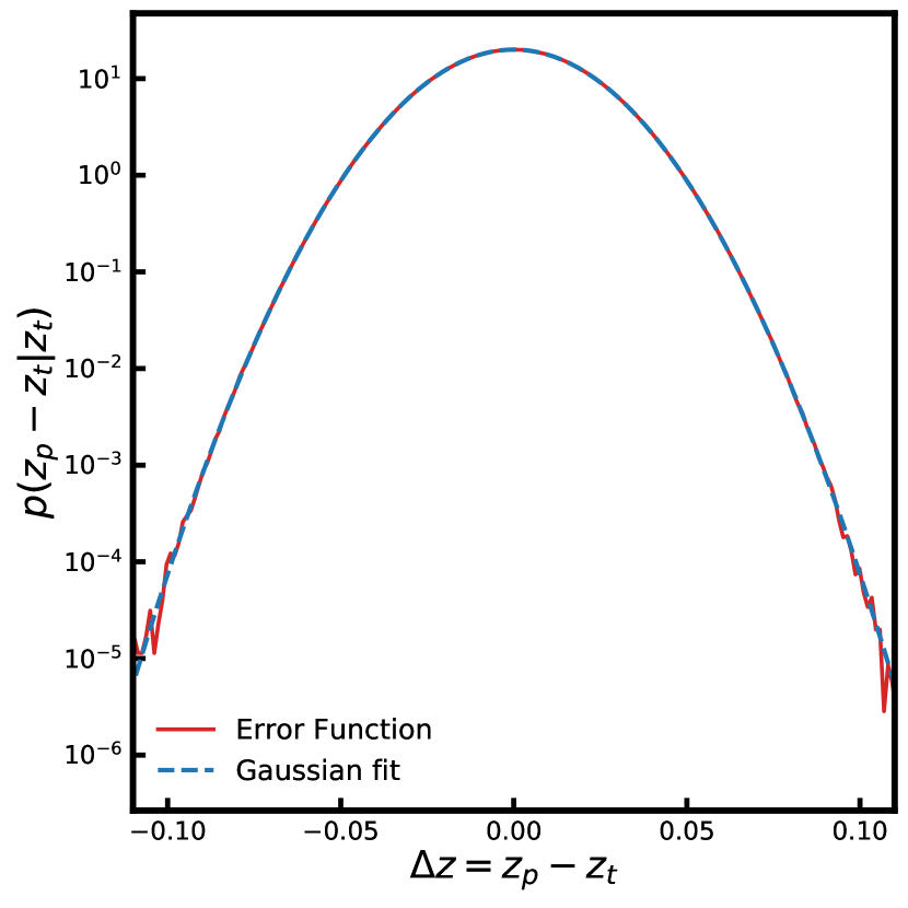
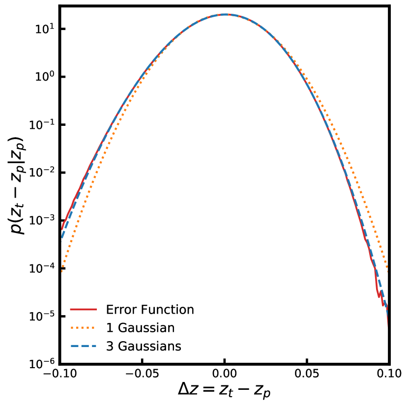
Figure 2: Left: Fit made to the error distribution $p(z_{p}-z_{t}|z_{t})$ with $\sigma_{0}=0.02$ (red solid line) using single Gaussian (blue dashed line). Right: Fit made to the error distribution $p(z_{t}-z_{p}|z_{p})$ with $\sigma_{0}=0.02$ (red solid line) using single Gaussian (orange dotted line) and sum of three Gaussians (blue dashed line).

The estimation of the true redshift distribution requires fitting the error function (i.e. either $p(z_{t}-z_{p}|z_{p})$ or $p(z_{p}-z_{t}|z_{t})$) with parametric functions. We have used a single Gaussian for $p(z_{p}-z_{t}|z_{t})$ and a sum of three Gaussian to fit $p(z_{t}-z_{p}|z_{p})$. Fig. 2 shows the quality of fit to the error functions with $\sigma_{0}=0.02$ and compares single Gaussian versus three Gaussians fit of $p(z_{t}-z_{p}|z_{p})$. The sum of three Gaussians provides a significantly better fit by accurately capturing the non-Gaussian wings of the error function. The uncertainties in these fits remain within $0.25\%$, and we do not expect these sub-per cent uncertainties to bias the power spectra or estimation of parameters.

In Fig. 3, we show the relative error, averaged over 300 simulations, of the redshift distribution reconstructed using the deconvolution method for the two cases of $\sigma_{0}=0.02\text{ and }0.05$. The reconstructed redshift distribution is within $\sim 2\%$ for the entire redshift range with maximum deviations occurring near boundaries possibly due to sharp cuts in the redshift distribution at $z=0$ and $z=3$ (section 3.2.2).

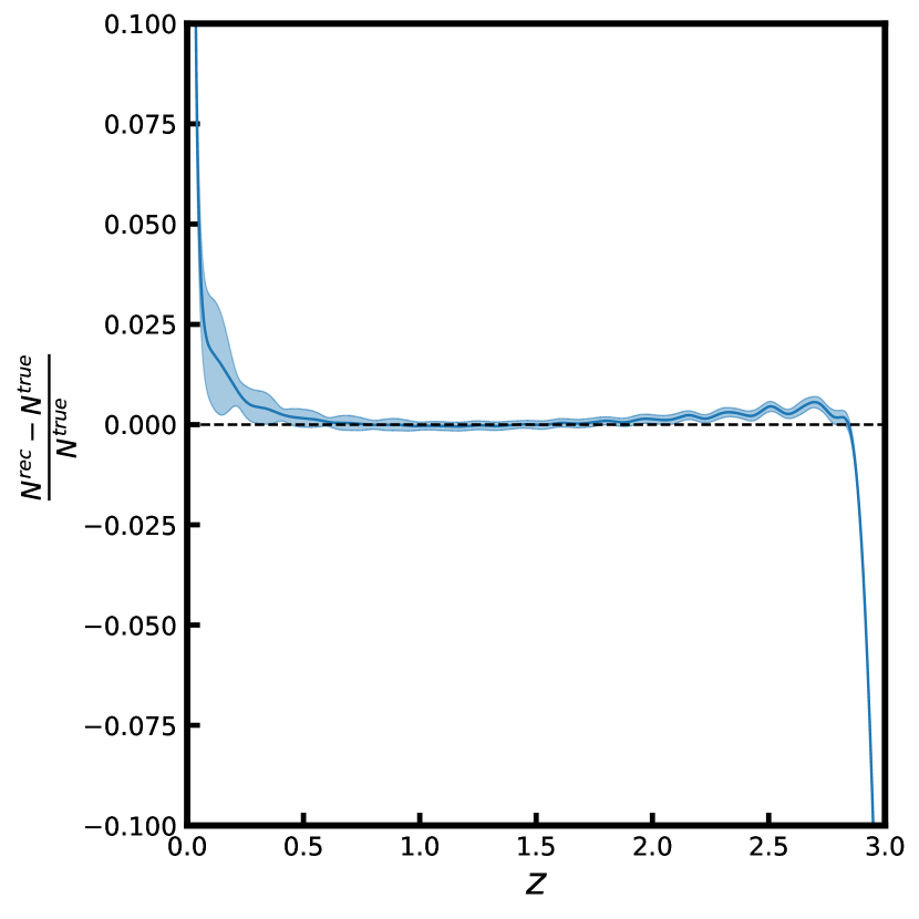
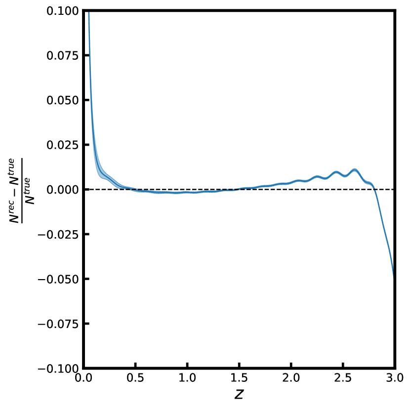
Figure 3: Average relative difference between the redshift distributions reconstructed using the deconvolution method and the true distribution for 300 simulations with left: $\sigma_{0}=0.02$ and right: $\sigma_{0}=0.05$. The shaded region represents the $1\sigma$ deviations in reconstruction between 300 simulations.

4.2 Power spectra from photometric datasets

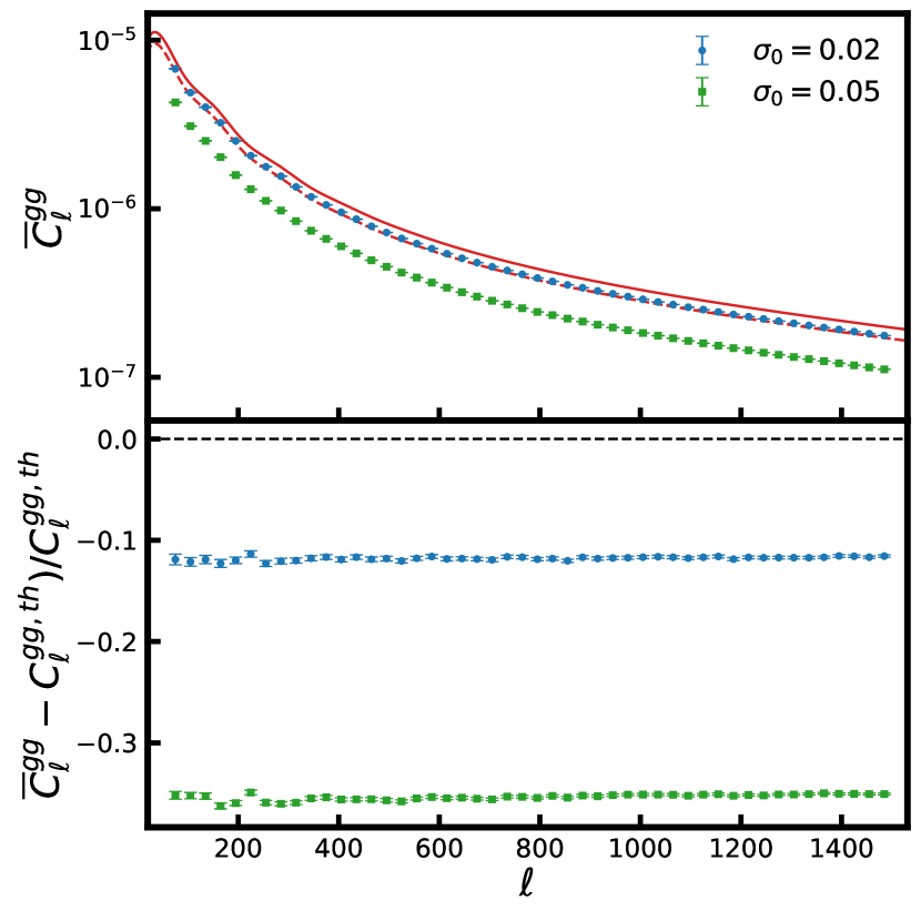
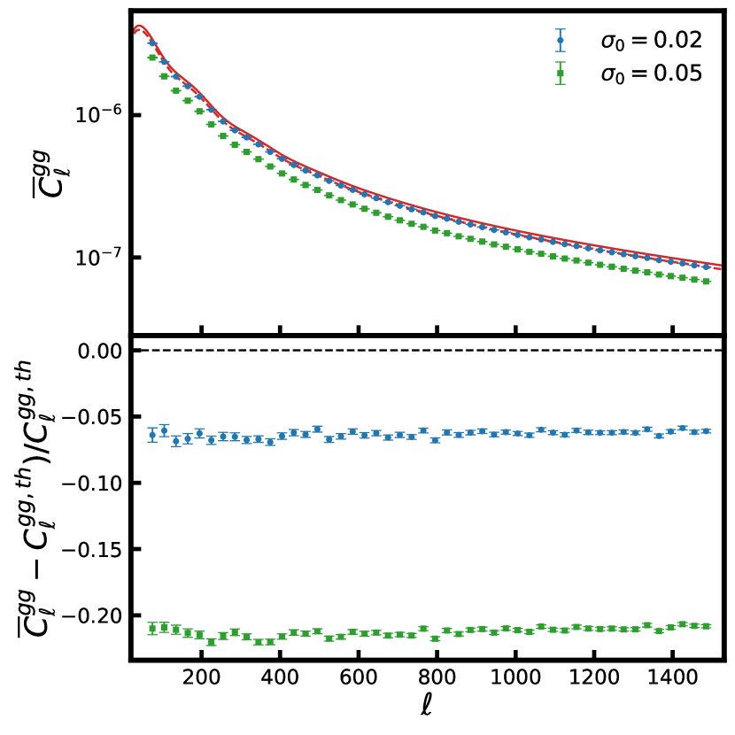
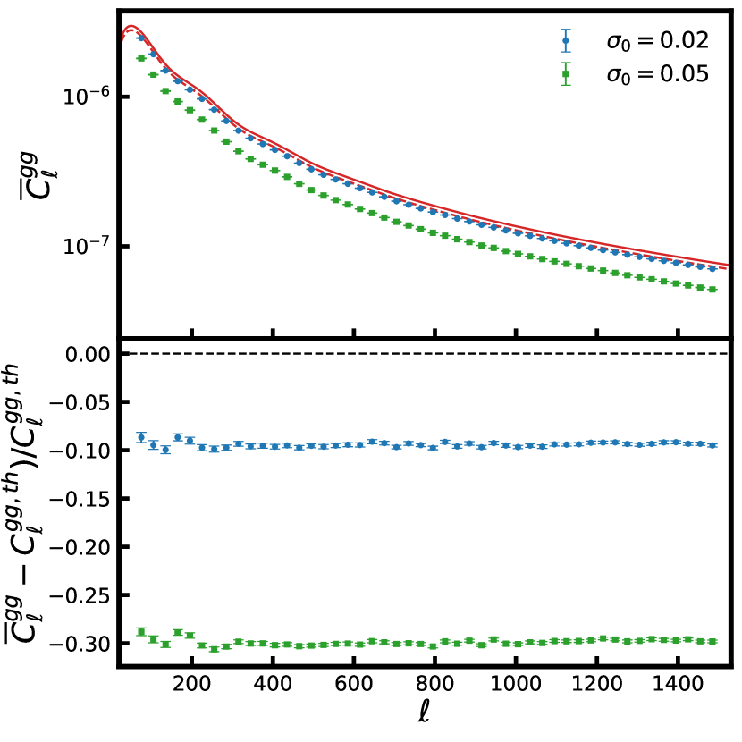
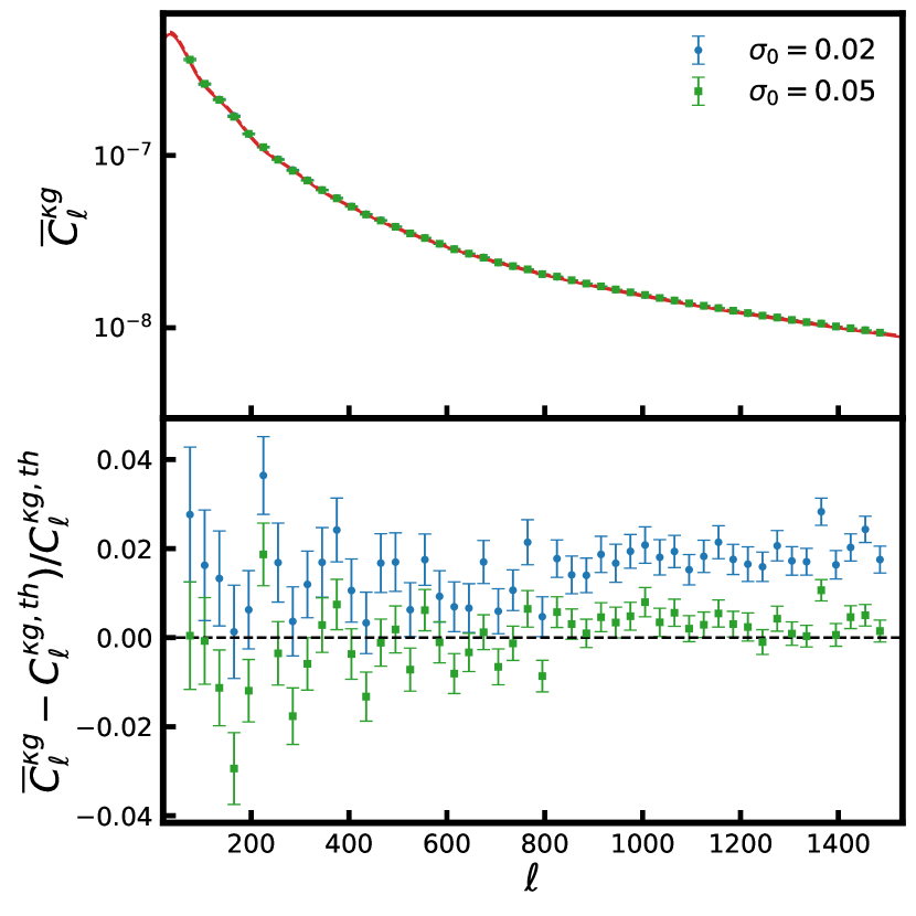
(a) Bin 5 ($0.8\leq z<1.0$)

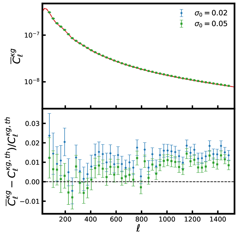
(b) Bin 6 ($1.0\leq z<1.4$)

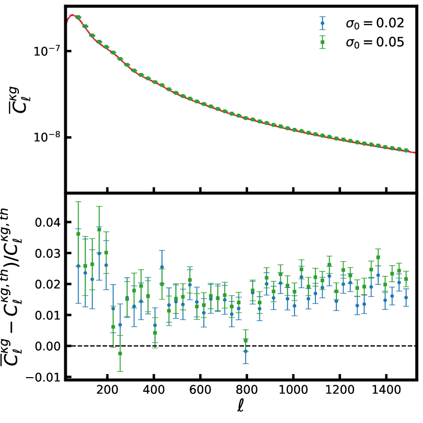
(c) Bin 7 ($1.4\leq z<1.8$)

Figure 4: Top: Average galaxy auto-power spectrum and bottom: cross-power spectrum reconstructed from 300 realisations of photometric datasets for three tomographic bins. The blue circles and green squares show the reconstructed power spectra for $\sigma_{0}=0.02\text{ and }0.05$, respectively. The solid and dashed red lines are the corresponding theoretical power spectra computed with redshift distributions estimated by the convolution method using Eq. (11). The error bars are computed from the covariance matrix of simulations using Eq. (8).

Here we present the power spectra for simulations with photometric redshift errors estimated using the method described in section 3.1. The noise-subtracted average galaxy auto-power spectra $(\overline{C}_{\ell}^{gg})$ and cross-power spectra between CMB lensing and galaxy over-density $(\overline{C}_{\ell}^{\kappa g})$ extracted from photometric datasets for three tomographic bins are shown with blue circles (for $\sigma_{0}=0.02$) and green squares (for $\sigma_{0}=0.05$) in Fig. 4. The red solid and dashed lines are the theoretical power spectra computed using the redshift distributions estimated by the more common convolution method (section 3.2.1) for $\sigma_{0}=0.02\text{ and }0.05$, respectively. We also present the relative difference between the extracted average power spectra and their theoretical expectations. The relative difference between estimated and theoretical power spectra for the other tomographic bins are shown in Appendix C.

The estimated galaxy auto-power spectra are smaller than expectations in every tomographic bin, with offsets varying between $2-15\%$ for $\sigma_{0}=0.02$ and between $15-40\%$ for $\sigma_{0}=0.05$. The cross-power spectra show comparatively smaller biases, i.e. $<5\%$ in every tomographic bin for both $\sigma_{0}=0.02$ and $\sigma_{0}=0.05$. We find similar offsets when the true redshift distributions (and hence the theoretical power spectra) are computed using the deconvolution method (following Eq. (17)). This shows that the offset in the power spectra is not related to the method of choice. Furthermore, since larger photometric redshift scatters lead to larger deviations in the power spectra, this confirms that the origin of these offsets is rooted in the leakage of objects from one redshift bin to the other due to photometric redshift errors. These deviations will also impact the estimation of parameters from the power spectra.

5 Leakage correction through scattering matrix

Due to errors in photometric redshifts, a fraction of galaxies observed in a given photometric redshift bin come from other redshift bins. The leakage of objects across redshift bins changes the strength of correlation in a tomographic analysis as well as results in non-zero correlation between different redshift bins. In this section, we attempt to counter the redshift bin mismatch of objects through the scattering matrix. If we divide galaxies into $n$ tomographic bins, then Zhang et al. (2010) have shown that noise subtracted galaxy auto-power spectrum between $i^{\text{th}}$ and $j^{\text{th}}$ photometric bins, $C_{ij}^{gg,\text{ph}}$, are related to the noise subtracted galaxy auto-power spectra from the $k^{\text{th}}$ true redshift bin $C^{gg,\text{tr}}_{kk}$ by

$$C_{ij}^{gg,\text{ph}}(\ell)=\sum\limits_{k}P_{ki}P_{kj}C_{kk}^{gg,\text{tr}}(\ell)$$ (21)

when there are no cross-correlations between true redshift bins. Eq. (21) has a generalized form for the case with true redshift bins having non-zero correlations, however, using disjoint true redshift bins significantly reduces the complexity. The elements of the scattering matrix $P_{ij}$ are defined as the ratio $N_{i\to j}/N_{j}^{\text{ph}}$, where $N_{i\to j}$ is the number of galaxies coming from $i^{\text{th}}$ true redshift bin to $j^{\text{th}}$ photometric bin and $N_{j}^{\text{ph}}$ is the total number of galaxies in the $j^{\text{th}}$ photometric bin. This definition also produces a natural normalisation $\sum\limits_{i}P_{ij}=1$. A similar relation for the cross-power spectra between galaxy over-density in redshift bin $i$ and CMB lensing convergence can be obtained as

$$C_{i}^{\kappa g,\text{ph}}(\ell)=\sum\limits_{k}P_{ki}C_{kk}^{\kappa g,\text{tr}}(\ell)$$ (22)

If we collect $P_{ij}$ as elements of the scattering matrix $P$, then we can compactly write

$$C^{gg,\text{ph}} =P^{\text{T}}C^{gg,\text{tr}}P$$ (23)

$$C^{\kappa g,\text{ph}} =P^{\text{T}}C^{\kappa g,\text{tr}}$$ (24)

where $P^{\text{T}}$ denotes the transpose of matrix $P$. Eqs. (23-24) show that the redistribution of galaxies across redshift bins due to photometric redshift errors results in a non-trivial relation between the photometric and true power spectra, weighted by the elements of the scattering matrix. Thus to properly mitigate the effects of leakage on power spectra, a precise estimation of the scattering matrix is necessary.

Zhang et al. (2017) proposed an algorithm to solve problems similar to Eq. (23) based on the Non-negative Matrix Factorization (NMF) method, that simultaneously approximates the matrices $P$ and $C^{gg,\text{tr}}$. However, the NMF method proves to be computationally challenging for cases with a large number of tomographic and multipole bins. Here, we propose an alternative method for fast and efficient computation of the scattering matrix based on the true and photometric redshift distributions. We first estimate the true redshift distribution, $\frac{\mathrm{d}N(z_{t})}{\mathrm{d}z_{t}}$, for the entire redshift range following Eq. (14) and then we use Eq. (17) to compute the redshift distribution $\frac{\mathrm{d}N^{i}(z_{p})}{\mathrm{d}z_{p}}$ for every tomographic bin $i$. The elements of the scattering matrix $P_{ij}$ can then be computed directly by using the relation

$$P_{ij}=\frac{\int\limits_{z_{min}^{j}}^{z_{min}^{j+1}}\mathrm{d}z_{p}\frac{\mathrm{d}N^{i}}{\mathrm{d}z_{p}}}{\int\limits_{z_{min}^{j}}^{z_{min}^{j+1}}\mathrm{d}z_{p}\frac{\mathrm{d}N}{\mathrm{d}z_{p}}}$$ (25)

where $\frac{\mathrm{d}N}{\mathrm{d}z_{p}}$ is the observed photometric redshift distribution of galaxies and $z_{min}^{j}$ is the lower limit of the $j^{\text{th}}$ redshift bin. Our method of computing the elements of the scattering matrix is significantly faster than the NMF method and is only subject to accurate estimation of the error distribution as well as true redshift distribution.

Fig. 5 shows the performance of estimation of the scattering matrix from our proposed method using redshift distributions, for the two cases of $\sigma_{0}=0.02\text{ and }0.05$. The average value of the scattering matrix $\langle P\rangle$ and its standard deviation $\sigma(P)$ averaged over $300$ simulations are shown in the top and middle panels of Fig. 5, respectively. We note that the scattering matrix elements corresponding to the first true redshift bin have the maximum standard deviation. This behaviour is expected as the objects near $z=0$ do not strictly follow convolution as discussed in section 3.2.2. The accuracy of the estimation of the scattering matrix can be verified using true scattering matrix $P^{\text{True}}$ computed based on exactly counting the number of objects moving from one redshift bin to the other in the catalogue generated by the FLASK code. In the bottom panel of Fig. 5, we show the difference between the scattering matrix computed from our method and $P^{\text{True}}$, averaged over $300$ realisations. We find that $|P-P^{\text{True}}|<0.006$ for all elements of the scattering matrix, with maximum differences occurring in the first and last tomographic bins, i.e. near the boundaries of the redshift range simulated in our analysis. Hence, the overall precision and accuracy in the estimation of the scattering matrix is found to be good and can be used for correcting redshift bin mismatch for the power spectra.

Given an estimate of the true redshift distribution deconvoluted from the observed photometric redshift distribution and scattering matrix, the impact of redshift bin mismatch of objects can be corrected in two ways: either by transforming true theoretical power spectra $C^{\text{th,tr}}$ to $C^{\text{th,ph}}$ using Eqs. (23) and (24) and comparing it to the estimated photometric power spectra $\hat{C}^{\text{ph}}$, or by inverting Eqs. (23) and (24) to transform the estimated photometric power spectra $\hat{C}^{\text{ph}}$ to true power spectra $\hat{C}^{\text{tr}}$ and comparing it to the theoretical true power spectra $C^{\text{th,tr}}$. We use the former approach for figures showing the comparison of power spectra while the latter for the estimation of parameters.

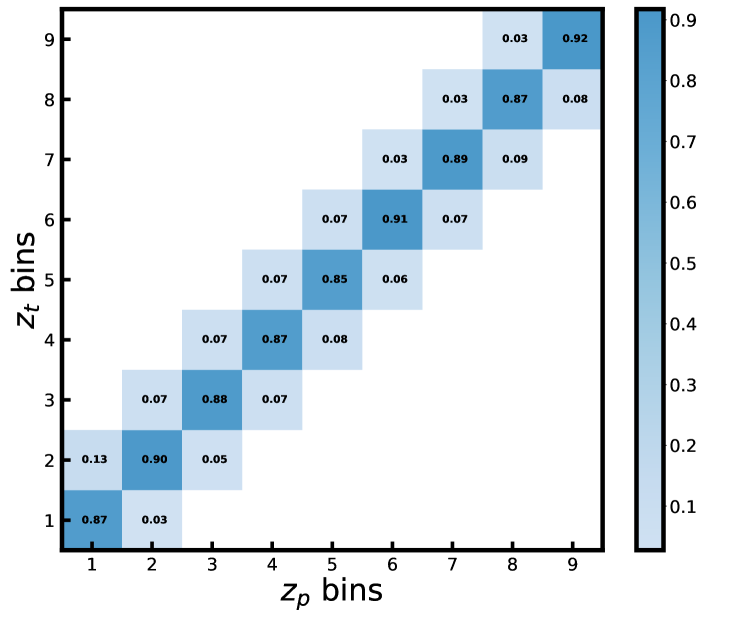
(a) $\langle P\rangle$

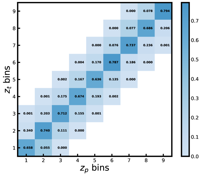
(b) $\langle P\rangle$

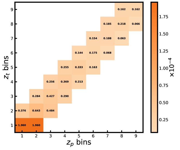
(c) $\sigma(P)$

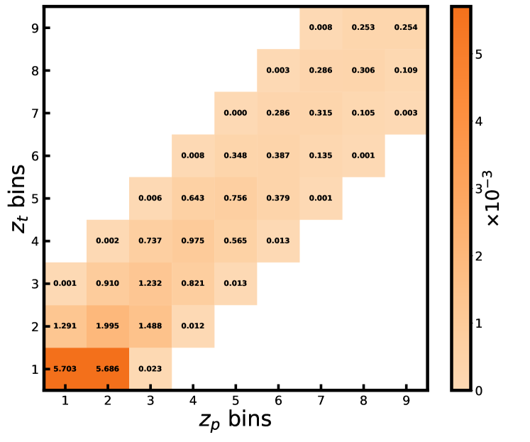
(d) $\sigma(P)$

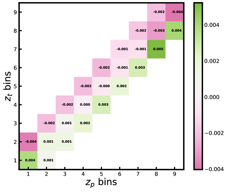
(e) $\langle P-P^{\text{True}}\rangle$

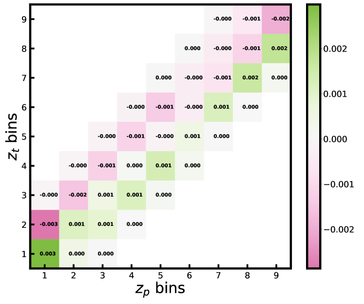
(f) $\langle P-P^{\text{True}}\rangle$

Figure 5: Performance of scattering matrix computed with the method described in section 5. Top: The average scattering matrix computed from 300 realisations, middle: its standard deviation, and bottom: the difference between scattering matrix computed from our method and true scattering matrix computed from simulated catalogues. Left column: scattering matrix computed for $\sigma_{0}=0.02$; Right column: scattering matrix computed for $\sigma_{0}=0.05$.

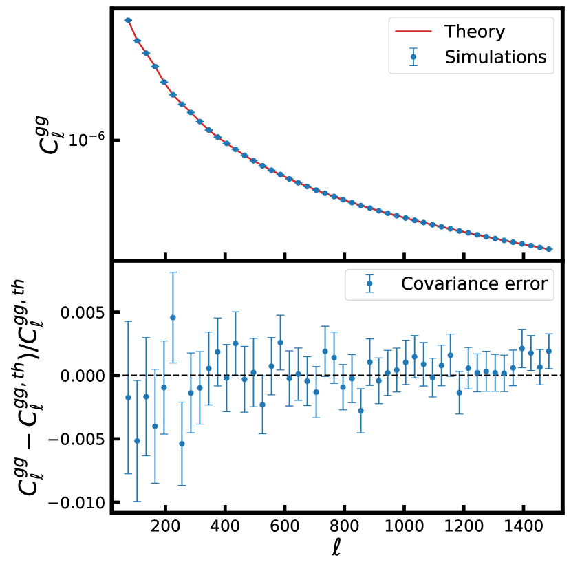
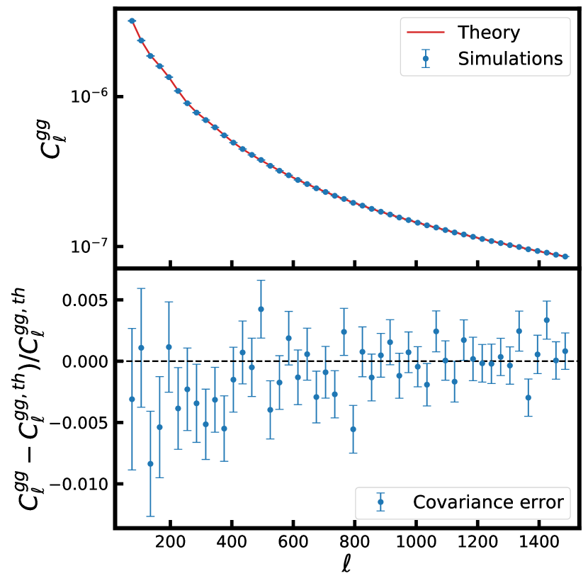
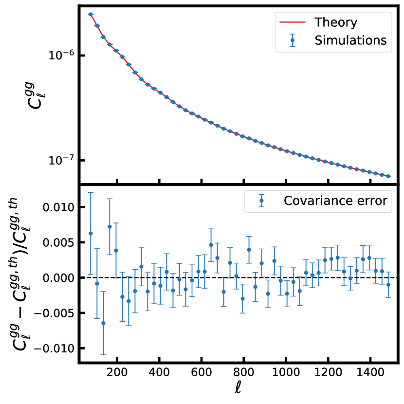
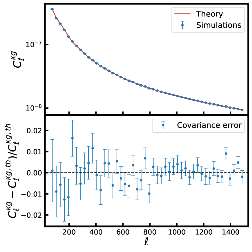
(a) Bin 5 ($0.8\leq z<1.0$)

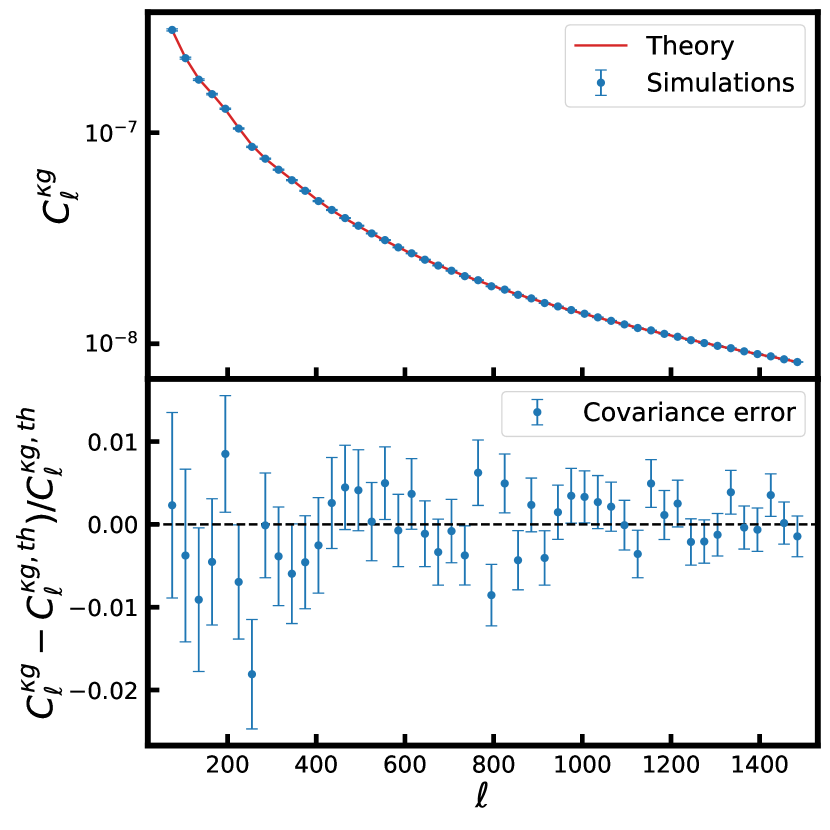
(b) Bin 6 ($1.0\leq z<1.4$)

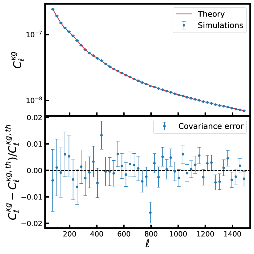
(c) Bin 7 ($1.4\leq z<1.8$)

Figure 6: Top: Average galaxy auto-power spectrum and bottom: cross-power spectrum reconstructed from $300$ realisations of photometric datasets with $\sigma_{0}=0.02$, shown for three tomographic bins. The red line represents the theoretical power spectrum corrected for redshift bin mismatch using Eqs. (23) and (24). The error bars are computed from the covariance matrix of simulations using Eq. (8).

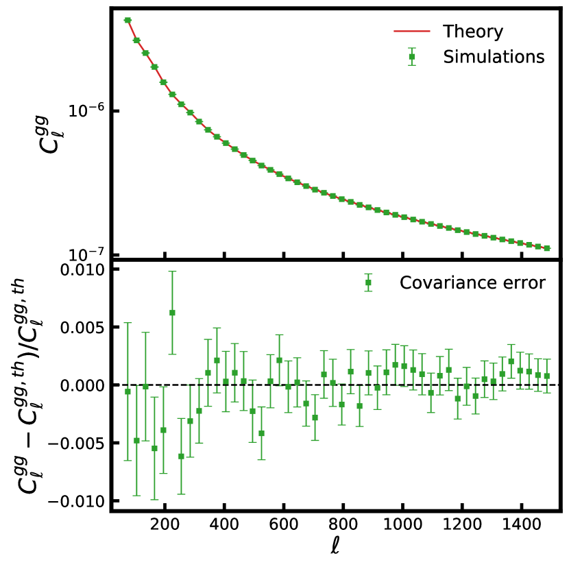
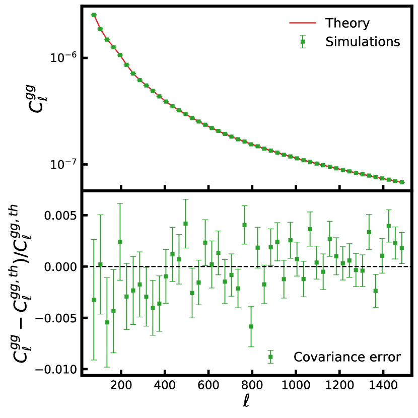
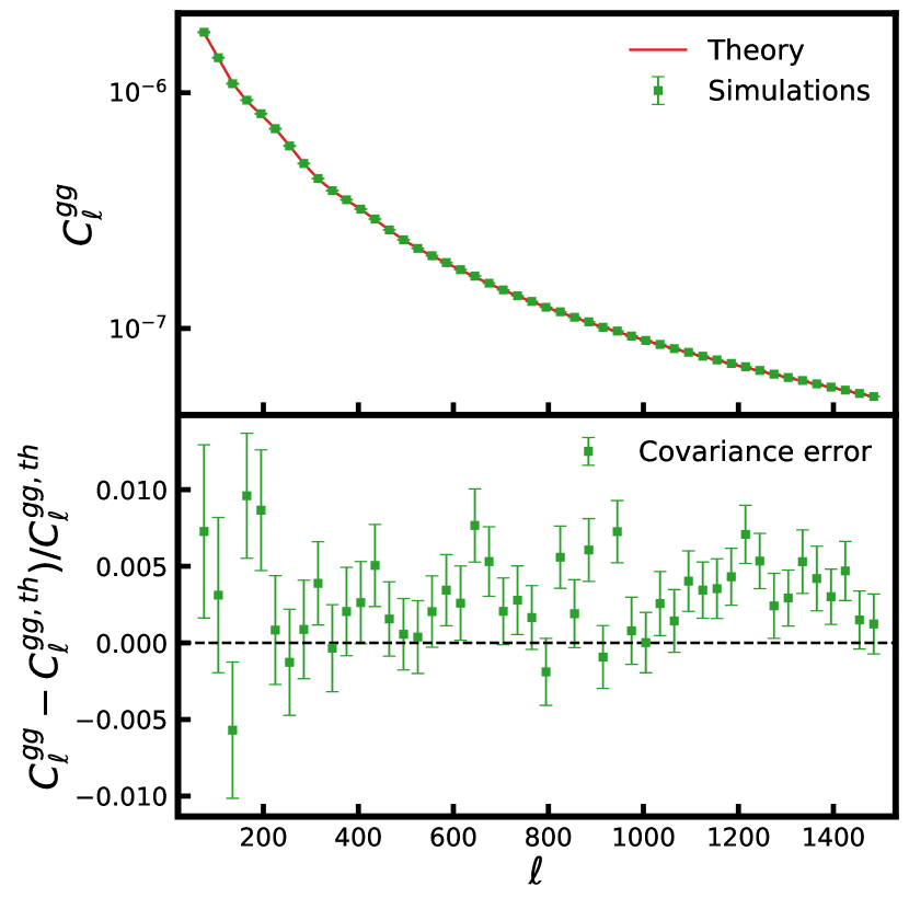
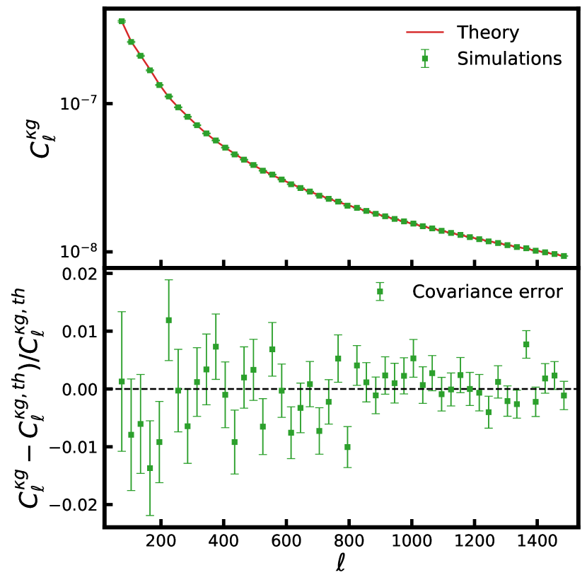
(a) Bin 5 ($0.8\leq z<1.0$)

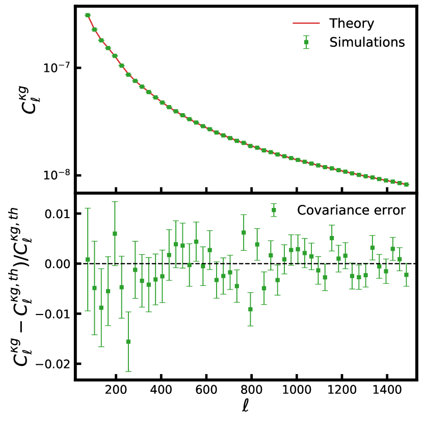
(b) Bin 6 ($1.0\leq z<1.4$)

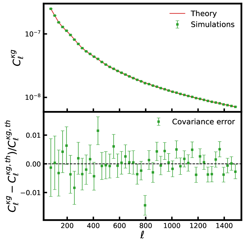
(c) Bin 7 ($1.4\leq z<1.8$)

Figure 7: Top: Average galaxy auto-power spectrum and bottom: cross-power spectrum reconstructed from 300 realisations of photometric datasets with $\sigma_{0}=0.05$, shown for three tomographic bins. The red line represents the theoretical power spectrum corrected for redshift bin mismatch using Eqs. (23) and (24). The error bars are computed from the covariance matrix of simulations using Eq. (8).

In Fig. 6 and 7, we show for the three tomographic bins shown in Fig. 4, comparison of noise-subtracted average estimated photometric power spectra with theoretical power spectra corrected for the bin mismatch leakage using Eqs. (23) and (24). The power spectra for other tomographic bins are presented in Appendix D. The theoretical power spectra after leakage correction agree completely with the estimated power spectra in all bins, except for the first and last tomographic bin. The disparity in the first and last bins results directly from the inaccuracy of the convolution method near the lower and upper bounds of the redshift distribution considered in the analysis. Nevertheless, we notice that even for those tomographic bins the agreement with corresponding theoretical power spectra improves.

6 Parameter estimation

In previous sections, we observed that the power spectra in every tomographic bin get biased due to the leakage of objects across redshift bins, which can be corrected by accurate estimation of the scattering matrix. In this section, we study the impact of leakage on the estimation of redshift dependent galaxy linear bias $b$ and amplitude of cross-correlation $A$ from tomographic bins, estimated using the Maximum Likelihood Estimation method discussed in section 3.3.

Before accounting for leakage, we estimate the galaxy linear bias and cross-correlation amplitude for every tomographic bin using the average galaxy power spectra and the average cross-power spectra estimated from photometric datasets. The theoretical power spectrum templates for tomographic bin $i$ are computed using Eq. (1) with the redshift distributions given by Eq. (11). To estimate parameters $b$ and $A$ after correcting for the redshift bin mismatch, we transform the extracted photometric power spectra ($\overline{C}^{gg,\text{ph}}$ and $\overline{C}^{\kappa g,\text{ph}}$) to true power spectra by inverting Eqs. (23) and (24). The theoretical power spectrum templates for likelihood estimation after leakage correction are computed by substituting Eq. (15) for the redshift distribution in Eq. (1). It is important to note that the photometric power spectra in tomographic analysis are a combination of true power spectra as represented in Eqs. (23) and (24). Thus, the galaxy linear bias in a photometric redshift bin will also be a combination of the galaxy linear bias from the true redshift bins. The estimation of parameters can also be performed directly over the estimated photometric power spectra by properly defining the covariance matrix in the likelihood function. However, transforming the estimated photometric power spectra to true power spectra for parameter estimation saves us from the complexities of defining the covariance matrix as well as reduces the computation time.

In Fig. 8 and 9, we compare the posterior distribution of parameters estimated from the average power spectra with $\sigma_{0}=0.02\text{ and }0.05$, respectively, for three tomographic bins before and after leakage correction. The lighter and darker shaded contour represents the $68\%$ and $95\%$ confidence intervals. The red lines mark the true values of galaxy bias and cross-correlation amplitude. The best-fit values of galaxy linear bias and cross-correlation amplitude from all tomographic bins with $\pm 1\,\sigma$ errors, estimated before and after leakage corrections, are quoted in Tables 2 and 3 for $\sigma_{0}=0.02\text{ and }0.05$, respectively. The column $b_{\text{true}}$ contains the true values of bias for every tomographic bin. The galaxy linear bias for every tomographic bin estimated from photometric datasets is smaller than their expected value for both $\sigma_{0}=0.02\text{ and }0.05$, whereas the amplitude of cross-correlation is consistently higher than the expected value of unity. However, both parameters become consistent with their expected values after correcting for redshift bin mismatch of objects. In Fig. 10 we show the variations in the redshift evolution of galaxy linear bias parameter due to the effects from redshift bin mismatch of objects for $\sigma_{0}=0.02\text{ and }0.05$. The black dashed line marks the fiducial evolution of the galaxy bias used in our simulations. The galaxy linear bias shows marginal deviations from its true values after correction with scattering matrix, and the amplitude of cross-correlation is perfectly consistent with its expected value of unity within $1\,\sigma$.

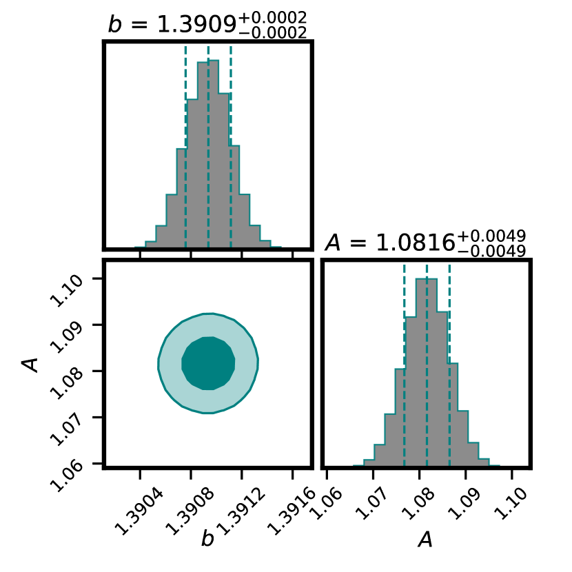
(a) Bin 5 ($0.8\leq z<1.0$)

(b) Bin 6 ($1.0\leq z<1.4$)

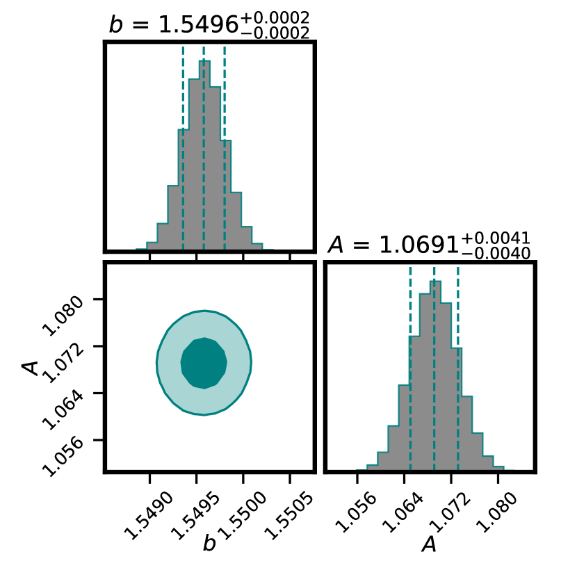
(c) Bin 7 ($1.4\leq z<1.8$)

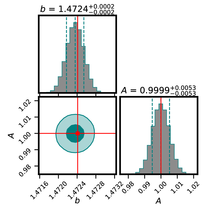
(d) Bin 5 ($0.8\leq z<1.0$)

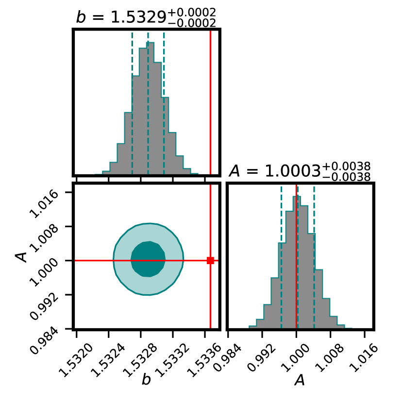
(e) Bin 6 ($1.0\leq z<1.4$)

(f) Bin 7 ($1.4\leq z<1.8$)

Figure 8: Parameter posteriors obtained from Maximum Likelihood Estimation performed over the average power spectra from $300$ simulations with $\sigma_{0}=0.02$, The top and bottom panels show the posteriors before and after leakage correction, respectively. The three vertical dashed lines are the median value of posterior and $\pm 1\sigma$ errors. The $68\%$ and $95\%$ confidence contours shown in darker and lighter shades, respectively. The red lines are the true values of parameters used for simulations.

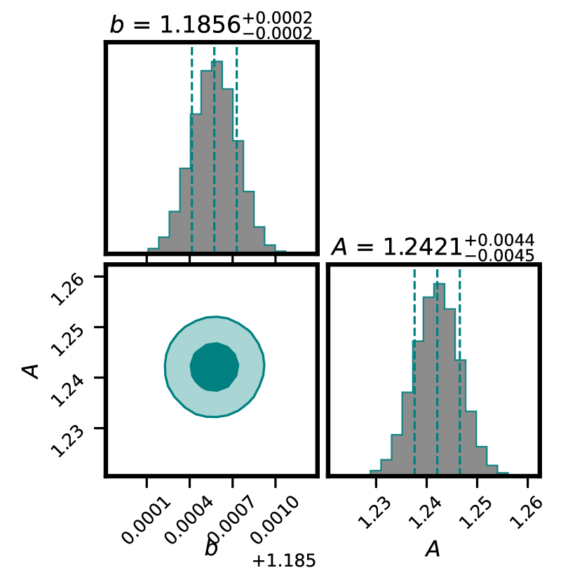
(a) Bin 5 ($0.8\leq z<1.0$)

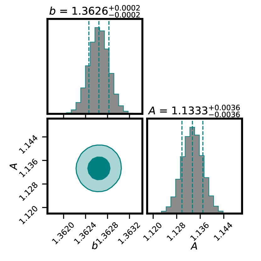
(b) Bin 6 ($1.0\leq z<1.4$)

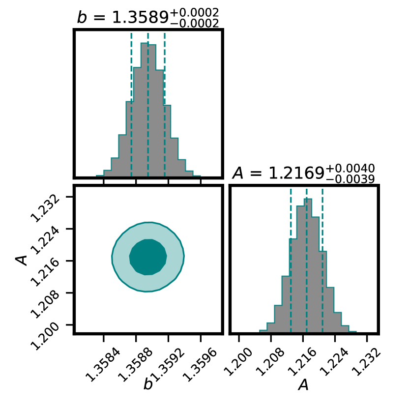
(c) Bin 7 ($1.4\leq z<1.8$)

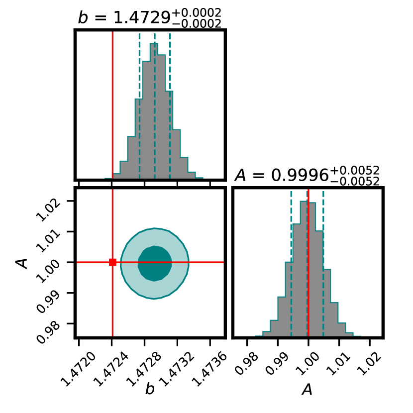
(d) Bin 5 ($0.8\leq z<1.0$)

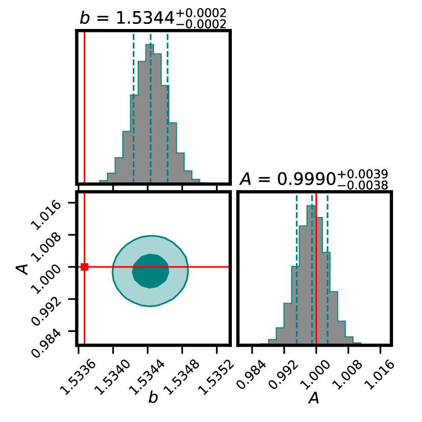
(e) Bin 6 ($1.0\leq z<1.4$)

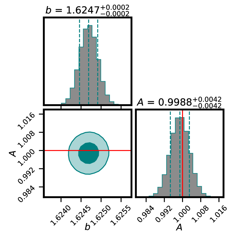
(f) Bin 7 ($1.4\leq z<1.8$)

Figure 9: Parameter posteriors obtained from Maximum Likelihood Estimation performed over the average power spectra from $300$ simulations with $\sigma_{0}=0.05$, The top and bottom panels show the posteriors before and after leakage correction, respectively. The three vertical dashed lines are the median value of posterior and $\pm 1\sigma$ errors. The $68\%$ and $95\%$ confidence contours shown in darker and lighter shades, respectively. The red lines are the true values of parameters used for simulations.

Table 2: Best fit values of galaxy linear bias $b$ and amplitude of cross-correlation $A$ from the average power spectra over $300$ simulations with $\sigma_{0}=0.02$, estimated before leakage correction and after correction through the scattering matrix approach. $b^{\text{true}}$ is the true value of bias for the tomographic bins. The error bars on the parameters correspond to the average of $300$ realizations.

$z$	$b^{\text{true}}$	No correction		With correction
		$b$	$A$	$b$	$A$
$[0.0,0.2)$	$1.3241$	$1.3552^{+0.0002}_{-0.0002}$	$1.0243^{+0.0110}_{-0.0110}$	$1.3357^{+0.0002}_{-0.0002}$	$0.9952^{+0.0124}_{-0.0125}$
$[0.2,0.4)$	$1.3541$	$1.3497^{+0.0002}_{-0.0002}$	$1.0269^{+0.0064}_{-0.0064}$	$1.3557^{+0.0002}_{-0.0002}$	$1.0014^{+0.0069}_{-0.0069}$
$[0.4,0.6)$	$1.3909$	$1.3623^{+0.0002}_{-0.0002}$	$1.0440^{+0.0053}_{-0.0054}$	$1.3911^{+0.0002}_{-0.0002}$	$0.9990^{+0.0058}_{-0.0057}$
$[0.6,0.8)$	$1.4307$	$1.3772^{+0.0002}_{-0.0002}$	$1.0645^{+0.0050}_{-0.0050}$	$1.4308^{+0.0002}_{-0.0002}$	$0.9998^{+0.0054}_{-0.0053}$
$[0.8,1.0)$	$1.4724$	$1.3909^{+0.0002}_{-0.0002}$	$1.0816^{+0.0049}_{-0.0049}$	$1.4724^{+0.0002}_{-0.0002}$	$0.9999^{+0.0053}_{-0.0053}$
$[1.0,1.4)$	$1.5337$	$1.4907^{+0.0002}_{-0.0002}$	$1.0465^{+0.0037}_{-0.0037}$	$1.5329^{+0.0002}_{-0.0002}$	$1.0003^{+0.0038}_{-0.0038}$
$[1.4,1.8)$	$1.6217$	$1.5496^{+0.0002}_{-0.0002}$	$1.0691^{+0.0041}_{-0.0040}$	$1.6223^{+0.0002}_{-0.0002}$	$1.0005^{+0.0042}_{-0.0042}$
$[1.8,2.2)$	$1.7118$	$1.5832^{+0.0003}_{-0.0003}$	$1.0963^{+0.0047}_{-0.0047}$	$1.7149^{+0.0003}_{-0.0003}$	$0.9986^{+0.0048}_{-0.0048}$
$[2.2,3.0)$	$1.8277$	$1.7318^{+0.0005}_{-0.0005}$	$1.0668^{+0.0047}_{-0.0047}$	$1.8137^{+0.0004}_{-0.0004}$	$1.0050^{+0.0048}_{-0.0047}$

Table 3: Best fit values of galaxy linear bias $b$ and amplitude of cross-correlation $A$ from the average power spectra over $300$ simulations with $\sigma_{0}=0.05$, estimated before leakage correction and after correction through the scattering matrix approach. $b^{\text{true}}$ is the true value of bias for the tomographic bins. The error bars on the parameters correspond to the average of $300$ realizations.

$z$	$b^{\text{true}}$	No correction		With correction
		$b$	$A$	$b$	$A$
$[0.0,0.2)$	$1.3241$	$1.2172^{+0.0002}_{-0.0002}$	$1.2081^{+0.0100}_{-0.0100}$	$1.3686^{+0.0002}_{-0.0002}$	$0.9872^{+0.0123}_{-0.0123}$
$[0.2,0.4)$	$1.3541$	$1.2288^{+0.0002}_{-0.0002}$	$1.0941^{+0.0059}_{-0.0058}$	$1.3555^{+0.0002}_{-0.0002}$	$1.0019^{+0.0069}_{-0.0069}$
$[0.4,0.6)$	$1.3909$	$1.2194^{+0.0002}_{-0.0002}$	$1.1354^{+0.0049}_{-0.0049}$	$1.3911^{+0.0002}_{-0.0002}$	$0.9986^{+0.0057}_{-0.0057}$
$[0.6,0.8)$	$1.4307$	$1.2088^{+0.0002}_{-0.0002}$	$1.1849^{+0.0045}_{-0.0046}$	$1.4311^{+0.0002}_{-0.0002}$	$0.9998^{+0.0054}_{-0.0054}$
$[0.8,1.0)$	$1.4724$	$1.1856^{+0.0002}_{-0.0002}$	$1.2421^{+0.0044}_{-0.0045}$	$1.4729^{+0.0002}_{-0.0002}$	$0.9996^{+0.0052}_{-0.0052}$
$[1.0,1.4)$	$1.5337$	$1.3626^{+0.0002}_{-0.0002}$	$1.1333^{+0.0036}_{-0.0036}$	$1.5344^{+0.0002}_{-0.0002}$	$0.9990^{+0.0039}_{-0.0038}$
$[1.4,1.8)$	$1.6217$	$1.3589^{+0.0002}_{-0.0002}$	$1.2169^{+0.0040}_{-0.0039}$	$1.6247^{+0.0002}_{-0.0002}$	$0.9988^{+0.0042}_{-0.0042}$
$[1.8,2.2)$	$1.7118$	$1.3692^{+0.0003}_{-0.0003}$	$1.2791^{+0.0046}_{-0.0046}$	$1.7138^{+0.0003}_{-0.0003}$	$0.9994^{+0.0048}_{-0.0048}$
$[2.2,3.0)$	$1.8277$	$1.6220^{+0.0005}_{-0.0005}$	$1.1614^{+0.0047}_{-0.0047}$	$1.8078^{+0.0004}_{-0.0004}$	$1.0082^{+0.0047}_{-0.0048}$

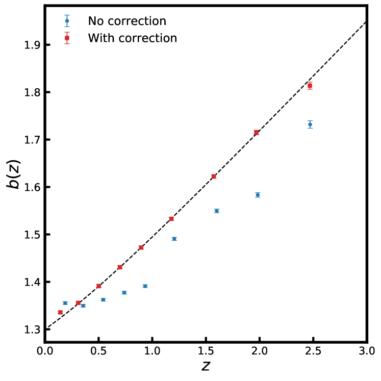
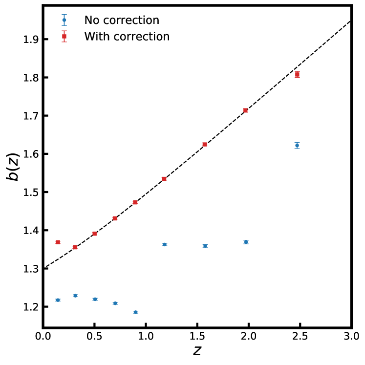
Figure 10: Comparison of galaxy linear bias parameter estimated from average of $300$ simulations before (blue circles) and after (red squares) correction for redshift bin mismatch of objects. The left figure is comparison for $\sigma_{0}=0.02$ and the right figure for $\sigma_{0}=0.05$. The error bars on parameters correspond to a single realization.

In Fig. 11, we show the relative difference between mean and fiducial value (in terms of standard deviation for a single realization) of galaxy linear bias and amplitude of cross-correlation for $\sigma_{0}=0.02$ (left column) and $\sigma_{0}=0.05$ (right column). The blue circles and red squares represent the parameter estimates before and after leakage correction, respectively. The error bars on the data points correspond to the average estimated power spectra. The top panel of Fig. 11 shows the relative difference for the galaxy linear bias parameter. Without properly accounting for the scatter of objects across redshift bins, the galaxy bias can deviate between $5-30\,\sigma$ when $\sigma_{0}=0.02$, and by $25-110\,\sigma$ when $\sigma_{0}=0.05$. Such large deviations on galaxy linear bias are visible because the errors from likelihood estimation (quoted in Tables 2 and 3) are between $0.15-0.5\%$ for a single realization. This shows that the estimates for the galaxy bias are very tightly constrained. The bottom panel of Fig. 11 shows the difference values for the amplitude of cross-correlation, which can deviate up to $\sim 1.2\,\sigma$ with $\sigma_{0}=0.02$, and up to $\sim 3.5\,\sigma$ when $\sigma_{0}=0.05$. As clearly conveyed by Fig. 11, the parameters galaxy linear bias and cross-correlation amplitude become consistent with their expected values after correcting for the effect of redshift bin mismatch of objects through our scattering matrix formalism.

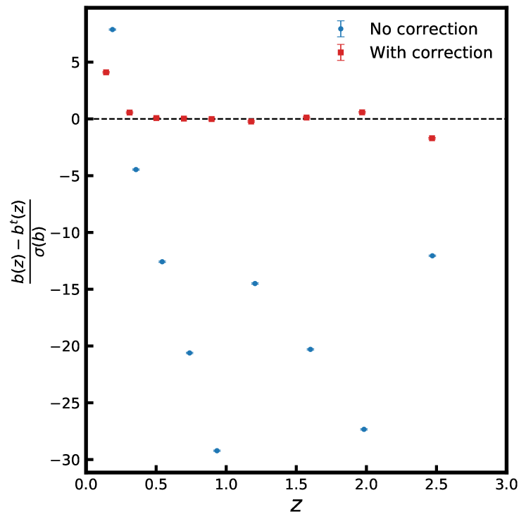
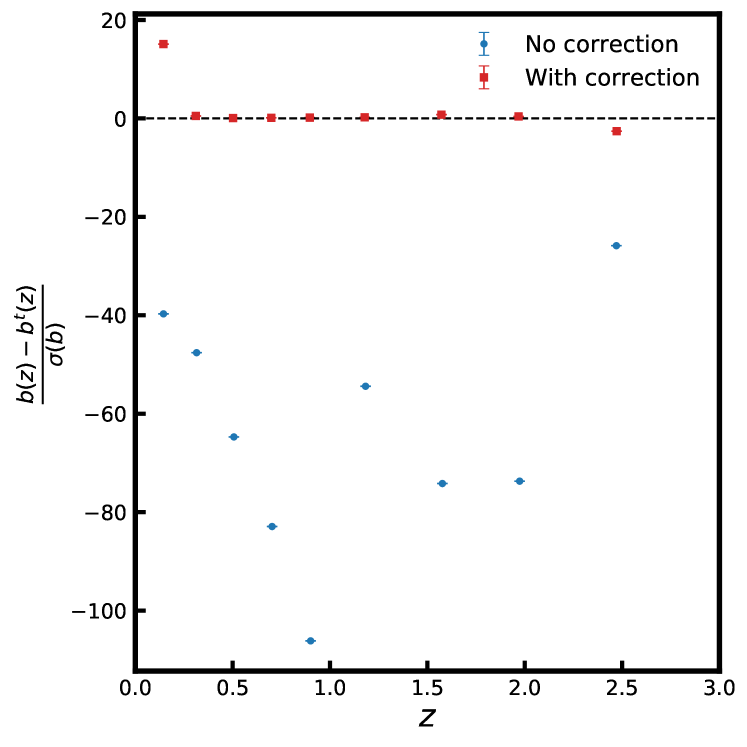
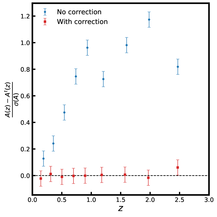
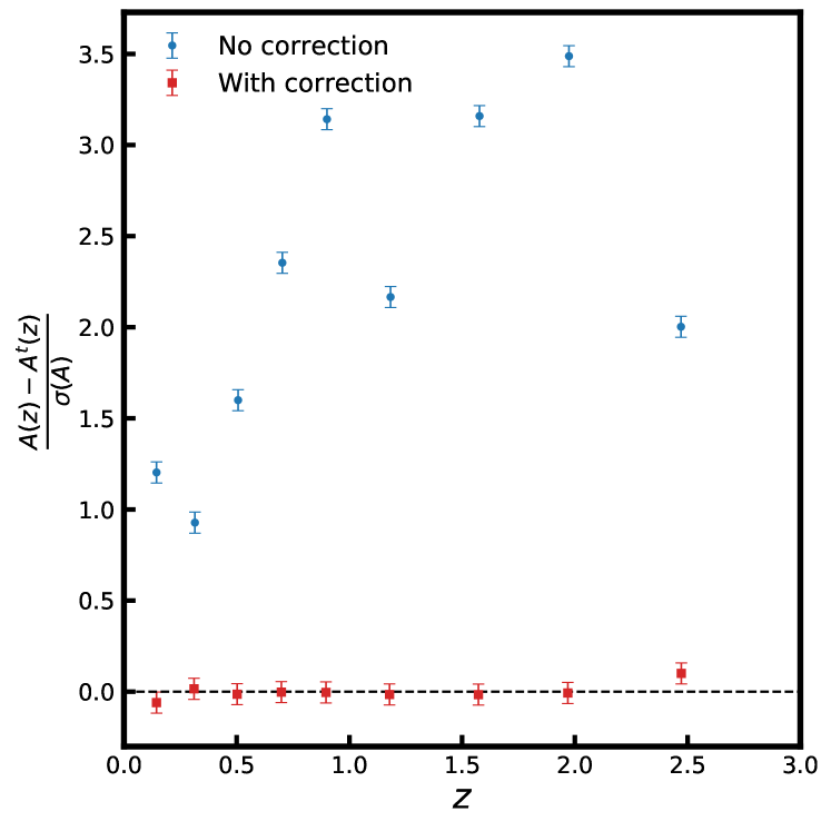
Figure 11: Comparison of top: relative difference for galaxy linear bias, and bottom: for cross-correlation amplitude estimated from the average power spectra, before (blue circles) and after (red squares) redshift bin mismatch correction. The left column is comparison for $\sigma_{0}=0.02$ and the right column for $\sigma_{0}=0.05$. The error bars on the data points corresponds to average spectra and the standard deviations $\sigma(b)$ and $\sigma(A)$ correspond to a single realization.

7 A note on $\sigma_{8}$ estimation

We have shown in section 6 that the scatter of objects across redshift bins can lead to a biased estimation of parameters, thus altering our inferences about the cosmological model. In this section, we will estimate the impact of leakage on the $\sigma_{8}$ parameter. Peacock & Bilicki (2018) proposed a method to compute the $\sigma_{8}$ parameter from the cross-correlation amplitude using the relation:

$$\sigma_{8}(z)=A(z)\,\sigma_{8,0}\,D(z)$$ (26)

where $\sigma_{8,0}$ is the value of $\sigma_{8}$ parameter at redshift $z=0$ and $D(z)$ is the linear growth function given by Eq. (5). We compute the value of $\sigma_{8,0}$ for our assumed background cosmology using CAMB software. In Fig 12, we show the impact of scattering of objects on $\sigma_{8}$ parameter computed using Eq. (26), for $\sigma_{0}=0.02\text{ (in left panel) and }0.05$ (on the right). The black dashed lines are the fiducial evolution of the $\sigma_{8}$ parameter with redshift. We measure a higher than expected value of $\sigma_{8}$ up to $\sim 1\,\sigma$ for $\sigma_{0}=0.02$ before correcting for redshift bin mismatch of objects. With $\sigma_{0}=0.05$, the $\sigma_{8}$ parameter is biased between $1-3\,\sigma$. As expected, the biases suffered by the amplitude of cross-correlation are reflected directly in the $\sigma_{8}$ parameter. We obtain an unbiased estimate of the $\sigma_{8}$ parameter after leakage correction, and thus it becomes crucial to correct the mismatch between different redshift bins in a tomographic analysis to get unbiased estimates of parameters.

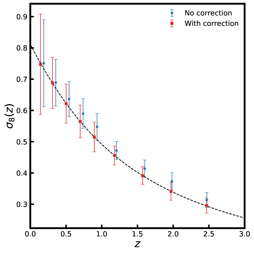
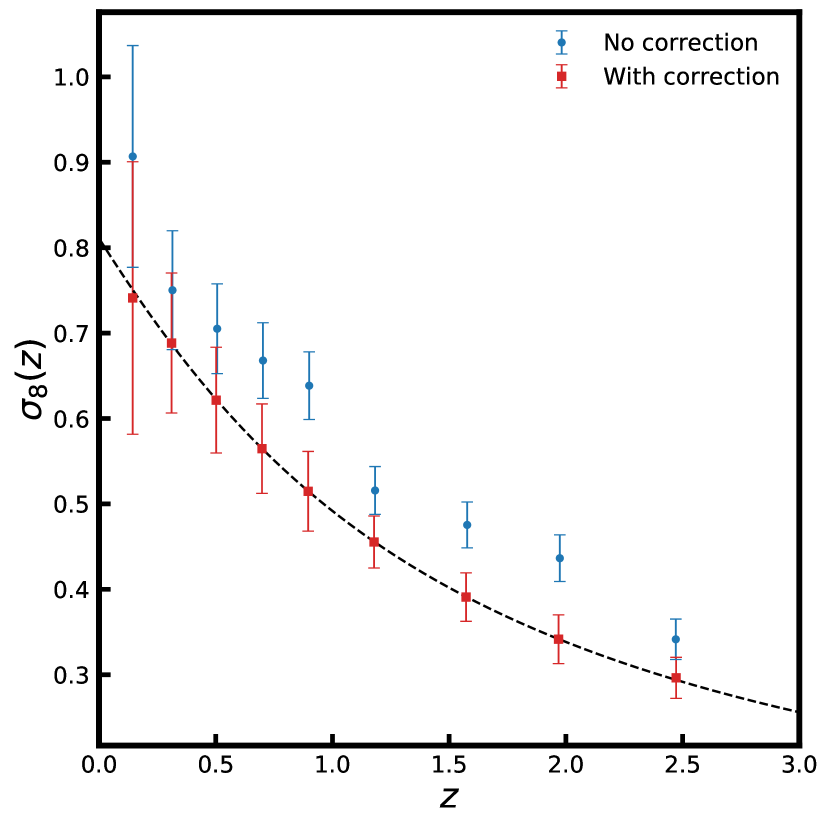
Figure 12: Comparison of $\sigma_{8}$ parameter estimated from the average power spectra of $300$ simulations, before and after leakage correction for $\sigma_{0}=0.02$ (left) and $\sigma_{0}=0.05$ (right). The black dashed line is the fiducial evolution of $\sigma_{8}$ parameter used during simulations. The error bars on parameters correspond to a single realization.

8 Summary and conclusions

We present the tomographic study of cross-correlations by performing simulations of Planck CMB lensing convergence and galaxy density field mimicking properties of LSST photometric survey. We use FLASK code to simulate log-normal fields and divide the galaxies into $9$ redshift bins. We consider photometric redshift errors with a standard deviation of $\sigma(z)=0.02(1+z)$ and $\sigma(z)=0.05(1+z)$ but do not include catastrophic redshift errors or photometric calibration errors, keeping them for future studies. In this sense, we generate an ‘ideal’ observational scenario in our simulations free from other systematics which is crucial to demonstrate the importance of redshift bin mismatch of objects. We compute galaxy auto-power spectrum and cross-power spectrum between galaxy over-density and CMB convergence fields and use these power spectra to estimate two parameters, the redshift dependent galaxy linear bias, $b$, and amplitude of cross-correlation, $A$, employing the maximum likelihood method.

We estimate the true redshift distribution from simulated photometric redshift distribution by the convolution method (section 3.2.1). In addition, we also estimate the true redshift distribution with the deconvolution method (section 3.2.2). The most important quantity to accurately recover the true redshift distribution is the precise estimation of the error distributions $p(z_{t}-z_{p}|z_{p})$ for convolution and $p(z_{p}-z_{t}|z_{t})$ for the deconvolution methods. We estimate the error functions with sub-percent accuracy ($<0.25\%$) by fitting a single Gaussian to $p(z_{p}-z_{t}|z_{t})$ and sum of three Gaussians to $p(z_{t}-z_{p}|z_{p})$ (shown in Fig. 2). We find the sum of Gaussians to accurately capture the peculiarities of the error function $p(z_{t}-z_{p}|z_{p})$ like non-Gaussian tails and higher peaks in the center.

The galaxy auto-power spectra measured from photometric datasets are found to be consistently smaller in every bin concerning their fiducial predictions. The offsets vary between $2-15\%$ for simulations with $\sigma(z)=0.02(1+z)$ and between $15-40\%$ for $\sigma(z)=0.05(1+z)$. The measured cross-power spectra are also biased with smaller deviations ($<5\%$) for both cases. The measured power spectra are inconsistent with their expectations due to the scattering of objects from one redshift bin to another due to photometric redshift errors. This conclusion is consistent with the fact that deviations are larger in the case of photometric redshift scatter $\sigma(z)=0.05(1+z)$.

To alleviate the differences in the power spectra, we implement the scattering matrix approach introduced by Zhang et al. (2010) to counter the effect of the redshift bin mismatch of objects. The scattering matrix describes the fraction of objects in a photometric redshift bin that comes from different true redshift bins. The power spectra in photometric redshift bins then transform as a linear combination of power spectra from different true redshift bins (Eqs. 23 and 24). Zhang et al. (2017) proposed an algorithm based on the Non-negative Matrix Factorisation method to solve similar numerical problems, however, this method is computationally challenging for a large number of data points in the power spectra and number of tomographic bins. To circumvent these challenges, we propose an alternative method for fast and accurate computation of the scattering matrix based on the reconstruction of the true redshift distribution by the deconvolution method (see section 5). We show in Fig. 5 that our new method to compute the scattering matrix is robust and only proves inefficient in the first tomographic bin due to a cut in the redshift distribution at boundary $z=0$. With a precise estimation of the scattering matrix, we correct the theoretical power spectra from the tomographic bins to compare with the estimated galaxy power spectra from simulated photometric datasets. Fig. 6 and 7 show that scattering matrix methodology makes the estimated power spectra consistent with the leakage corrected theoretical power spectra.

We quantify the impact of redshift bin mismatch of objects on the estimation of galaxy linear bias and amplitude of cross-correlation. To estimate parameters after leakage correction, we transform the estimated photometric power spectra to estimated true power spectra by inverting the Eqs. (23) and (24) (as described in section 6). The best-fit values of these parameters before and after leakage correction are quoted in Tables 2 and 3 for $\sigma(z)=0.02(1+z)$ and $\sigma(z)=0.05(1+z)$, respectively. Without accounting for the leakage, we estimate smaller values for the galaxy linear bias by $5-30\,\sigma$ when $\sigma_{0}=0.02$, and by $25-110\,\sigma$ when $\sigma_{0}=0.05$. Whereas the amplitude of cross-correlation is estimated higher than its fiducial value of unity up to $\sim 1.2\,\sigma$ with $\sigma_{0}=0.02$, and $\sim 3.5\,\sigma$ when $\sigma_{0}=0.05$. It is important to note here that the estimations of lower galaxy bias and higher amplitude are not to be generalized for every tomographic analysis. The offsets suffered by the power spectra and parameters estimated from photometric datasets in a tomographic study will depend strongly on the photometric redshift error distributions as well as the redshift distribution of objects. After correcting for leakage by using the scattering matrix, both parameters are very well constrained with their expected values.

The amplitude of cross-correlation is an indicator of the validity of the background cosmological model. Thus, without correcting for the bias resulting from photometric redshift errors, it will become inevitable to make wrong inferences when testing cosmological models with tomographic analyses. Other estimators frequently used to test the cosmological models, like the $D_{G}$ (Giannantonio et al., 2016) or $E_{G}$ (Pullen et al. 2016; Zhang et al. 2007) statistics, also employ the ratio of cross-power spectra to galaxy auto-power spectra and are, hence, prone to similar systematics. We study the relationship between the amplitude of cross-correlation and the more familiar $\sigma_{8}$ parameter in section 7. The $\sigma_{8}$ parameter deviates by up to $\sim 1\,\sigma$ when $\sigma(z)=0.02(1+z)$, and up to $\sim 3\,\sigma$ when $\sigma(z)=0.05(1+z)$. We show that the offsets suffered by the amplitude due to the scatter of objects are synonymous with the deviations in the $\sigma_{8}$ parameter. With next-generation galaxy surveys like Vera C. Rubin Observatory Legacy Survey of Space and Time (LSST, Ivezić et al. 2019; LSST Science Collaboration et al. 2009), Euclid (Laureijs et al., 2011), and Dark Energy Spectroscopic Instrument (DESI, Dey et al. 2019), the tomographic approach will emerge as a powerful tool to put stringent constraints on the validity of cosmological models. Hence, we propose that the scattering matrix approach developed and presented in this paper be strictly used for future tomographic studies.

Appendix A Validation of deconvolution method

In this section, we present the performance of the deconvolution method as described in section 3.2.2 using a toy example. We generate a fiducial redshift distribution by random sampling from the LSST photometric redshift distribution profile (Ivezić et al. 2019; LSST Science Collaboration et al. 2009) with mean redshift $0.9$, which we term as true distribution. We convolve the true distribution with a Gaussian distribution with $\mu=0.1,\sigma=0.02$ and call the resultant as the observed distribution. In the left column of Fig. 13, we show the true and observed distributions by blue and red solid lines, respectively. We attempt to show the robustness of our deconvolution method by applying it on un-smoothed distributions. In the right column of Fig. 13, we compare the true distribution (blue solid line) with the distribution recovered using our deconvolution method (red dashed line). The recovered distribution is in good agreement with the true redshift distribution, which validates our deconvolution method to reconstruct the true redshift distribution.

Figure 13: Left: True (blue solid line) and observed (red solid line) distributions for our toy example. Right: Comparison of the true redshift distribution (blue solid line) with the distribution recovered from deconvolution method (red dashed line). The recovered distribution is in excellent agreement with the true redshift distribution.

Appendix B Power spectra from true datasets

It is important to check for any systematics that may arise when preparing true datasets with the FLASK code. These systematics, if significant, will also affect any inferences made from photometric datasets. In Fig. 14 we show, for every tomographic bin, the relative difference between noise-subtracted average galaxy auto-power spectra estimated before adding photometric redshift errors and their theoretical expectation with error bars computed from Eq. (8). Fig. 15 and 16 present the relative difference for the cross-power spectrum and CMB convergence auto-power spectrum, respectively. The power spectra are consistent with their theoretical expectations in all tomographic bins and thus, the FLASK simulations are free from any internal systematics.

Figure 14: Relative errors in the average galaxy auto-power spectrum reconstructed from $300$ simulations generated by the FLASK code without adding photometric redshift errors. The error bars are computed from the covariance matrix of simulations using Eq. (8).

Figure 15: Relative errors in the average cross-power spectrum between galaxy over-density and CMB lensing reconstructed from $300$ simulations without adding photometric redshift errors. The error bars are computed from the covariance matrix of simulations using Eq. (8).

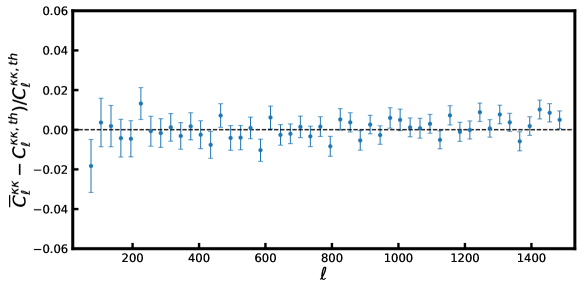
Figure 16: Relative errors in the average CMB convergence auto-power spectrum reconstructed from $300$ simulations. The error bars are computed from the covariance matrix of simulations using Eq. (8).

Appendix C Power spectra from photometric datasets

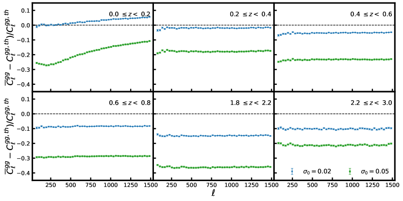
Figure 17: Average galaxy auto-power spectrum reconstructed from $300$ simulations after adding photometric redshift errors (complementary to Fig. 4). The error bars are computed from the covariance matrix of simulations using Eq. (8).

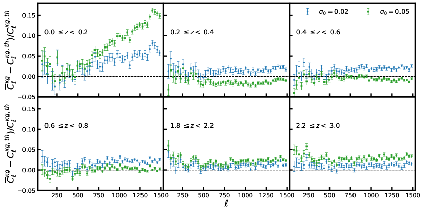
Figure 18: Average cross-power spectrum between galaxy over-density and CMB convergence reconstructed from $300$ simulations after adding photometric redshift errors (complementary to Fig. 4). The error bars are computed from the covariance matrix of simulations using Eq. (8).

Appendix D Power spectra after leakage correction

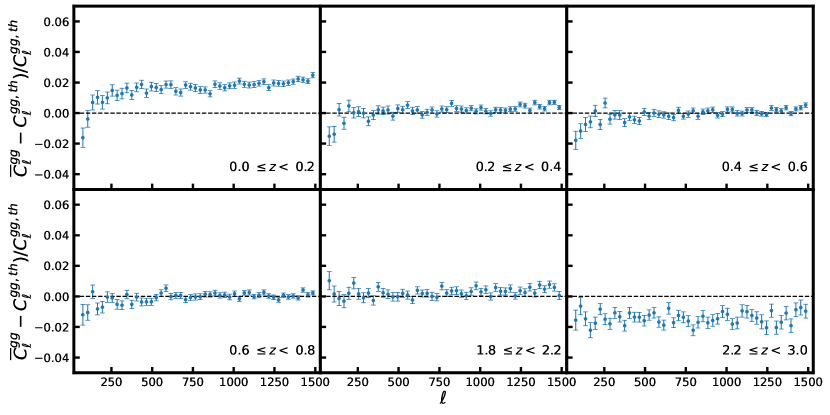
Figure 19: Average galaxy auto-power spectrum reconstructed from $300$ simulations of photometric datasets with $\sigma_{0}=0.02$, computed through scattering matrix (complementary to Fig. 6). The error bars are computed from the covariance matrix of simulations using Eq. (8).

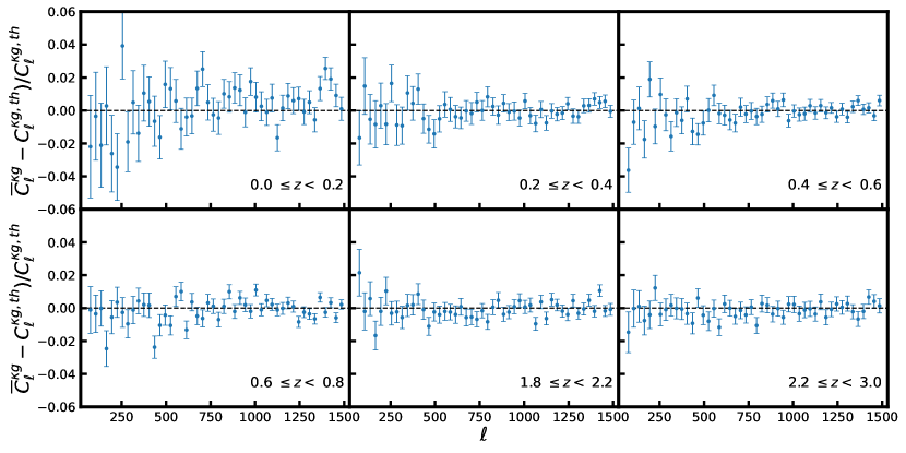
Figure 20: Average cross-power spectrum between galaxy over-density and CMB convergence reconstructed from $300$ simulations of photometric datasets with $\sigma_{0}=0.02$, shown for three tomographic bins computed through scattering matrix (complementary to Fig. 6). The error bars are computed from the covariance matrix of simulations using Eq. (8).

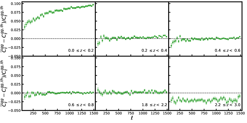
Figure 21: Average galaxy auto-power spectrum reconstructed from $300$ simulations of photometric datasets with $\sigma_{0}=0.05$, computed through scattering matrix (complementary to Fig. 7). The error bars are computed from the covariance matrix of simulations using Eq. (8).

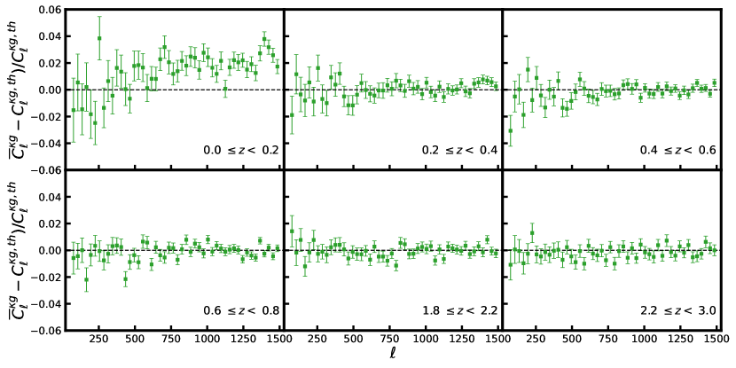
Figure 22: Average cross-power spectrum between galaxy over-density and CMB convergence reconstructed from $300$ simulations of photometric datasets with $\sigma_{0}=0.05$, shown for three tomographic bins computed through scattering matrix (complementary to Fig. 7). The error bars are computed from the covariance matrix of simulations using Eq. (8).