Bayesian imputation of revolving doors

Abstract

Political scientists and sociologists study how individuals switch back and forth between public and private organizations, for example between regulator and lobbyist positions, a phenomenon called “revolving doors”. However, they face an important issue of data missingness, as not all data relevant to this question is freely available. For example, the nomination of an individual in a given public-sector position of power might be publically disclosed, but not their subsequent positions in the private sector. In this article, we adopt a Bayesian data augmentation strategy for discrete time series and propose measures of public-private mobility across the French state at large, mobilizing administrative and digital data. We relax homogeneity hypotheses of traditional hidden Markov models and implement a version of a Markov switching model, which allows for varying parameters across individuals and time and auto-correlated behaviors. We describe how the revolving doors phenomenon varies across the French state and how it has evolved between 1990 and 2022.

Keywords: Bayesian Binary Markov Switching Model, GLM/GAM Markov Model, Data Augmentation, Revolving Doors, France

1 Motivation

Studying revolving doors is an especially hard problem for sociologists and political scientists, as it requires collecting numerous and hard-to-access data points. Compared to studying tenure length in political office or administration, it requires information about the positions someone might occupy before and after their time in office. This is sometimes done for personal histories before arriving in a position of power and is often called prosopography, but is even less often done for positions occupied after. Even when significant resources are devised to systematically collect career trajectories, data availability remains an impassable limiting factor. To ensure all data for a certain elite group has been collected, researchers often focus only on the most selective and visible portion of them, which reduces the array of groups that are available to traditional elite research.

Our main intuition is that work trajectories contain a logic, a structure, and that it is not necessary to observe everything about everyone to draw meaningful conclusions about collective behavior such as the state of revolving doors. If it is expected that an individual, working at the top of a certain field such as the state, would often leave digital or administrative traces of their activity, not observing such traces after a given point in time could be interpreted as a signal that they are not present in this field anymore. Knowing the cases in which such a conclusion can be drawn has to be inferred from data, and this problem justifies our mathematical framework. In essence, we introduce a certain class of latent models to enable the distinction between the actual trajectory someone might have, and the observed traces we have at our disposal to document it.

We study the problem of revolving doors broadly defined, as the description of mobility patterns between public organizations with considerable regulatory and executive power and the private sector. This application is conducted for the French case, on the 1990-2022 period, on two populations of civil servants of multiple thousands of individuals. We show that Markov switching models applied to this case are sufficiently expressive to actually replicate and enhance trajectory data well, while remaining very interpretable, enabling the direct testing of substantive research hypotheses from the literature. We test, on the one hand, whether public-private paths have become more frequent or not in the past 30 years; and we perform on the other hand a comparison across the main public organizations across the French state.

2 Setting

2.1 Problem

We consider the trajectories of individuals through time $t=1,...,T$. Time is discretized, and in our application, an increment by one unit corresponds to a 6-month period: $t=1$ corresponds to January-June 1990, and $T=68$ corresponds to July-December, 2022. This choice of granularity is the result of a tradeoff between computing time and precision, and it would be possible to choose a finer, 1-month period precision. For each individual $i$ (for $i=1,...,I$), we consider three quantities:

• the trajectory of individual $i$ between the public and the private sectors is represented by a discrete time series $\boldsymbol{X}=(X^{i}_{t})_{t}\in\{0,1\}$. We denote $X^{i}_{t}=0$ if individual $i$ holds a public sector position at time $t$, and $X^{i}_{t}=1$ if they hold a private sector position. This time series is partially observed. Our inference procedure will rely on data augmentation of the non-observed values.

• French public servants leave “traces”: for example, nomination to a new public position is recorded in the Journal Officiel, and this is one of the traces we consider. We model traces by a discrete time series $\boldsymbol{Y}=(Y_{t}^{i})_{t}\in\{0,1\}$, with $Y^{i}_{t}=1$ if individual $i$ has left at least one trace in an administrative archive at time $t$, and $Y^{i}_{t}=0$ otherwise.

• Each individual is further described by a vector $W^{i}_{t}$ of exogenous covariates, for example coding the type of civil servant we are interested in.

The principal goal of the problem is to describe the marginals of $X^{i}_{t}$ even when not observed, and to infer parameters regarding the behavior of this time series. A side problem consists of realistically modeling the relationship between the trajectories ($X_{t}^{i}$) and traces $(Y_{t}^{i})$ time series, as misspecification there could be propagated to the main problem and lead to erroneous estimates. As it stands, the problem is very similar to the classical unsupervised Bayesian hidden Markov model, but solving well the side problem will require to relax certain hypotheses.

2.2 Data sources

Our main data source is the “Journal officiel”, an administrative record with a significant legal value that includes new pieces of regulation, executive decisions and nominations. The nomination power in France is shared between the president and the prime minister, under the scrutiny of the Parliament, and this source documents nominations for many top-level positions in public organizations. It also includes, in certain cases, information about promotions, other career changes (like retirement) and decisions taken by authorities that might involve named civil servants. Importantly, certain key positions are systematically described, and this source can thus be used to define exhaustive and representative populations. However, not all public positions are described, and of course, positions in the private sector are by default not present in this record. This can make the identification of revolving door patterns difficult. The source was digitized starting in 1990, and this defines our temporal frame (1990-2022). It is this source we refer to when we mention that a trace was found at a certain time point $t$ for an individual $i$ and so $Y_{t}^{i}=1$.

A second data source is based on the website LinkedIn. LinkedIn is social media platform oriented towards professional networking, where users describe their past working experience on their profile. As we will see, many managers, both in the public and private sectors have a profile, but not the entirety of the population. In addition, as this data is auto-biographical, individuals may choose to not include all relevant information: there are notable gaps in profiles, which means that even if someone has a profile, there still might be missing data we ought to simulate. It is this source we refer to when we mention that the trajectory of an individual $i$ was observed at a certain time point $t$ and so $X_{t}^{i}$ is known.

2.3 Populations definition

In this article, we describe two populations of high civil servants: former students of the National School of Administration (Ecole Nationale d’Administration, hereafter ENA), and members of a select list of powerful services. To assemble the data, we queried all traces of the Journal officiel linked to the corresponding organizations and manually crafted a rule-based approach to only keep those that define membership. The full decision tree aims to fit as best as possible accounts from applied researchers and can be found in the appendix.

Each individual $i$ is modeled with $(X_{t}^{i})_{t},(Y_{t}^{i})_{t}$, on an interval $[T_{min}^{i},T_{\max}^{i}]$. We let $T_{\min}^{i}$ be their first membership-defining trace. If the individual has a trace that states they retired, we use that date for $T_{\max}^{i}$; else we let $T_{\max}^{i}=T$, where $T$ corresponds to our last observation time (July-December 2022).

2.3.1 Population 1: former students of ENA

The National School of Administration ENA was founded in 1945 to select and train high civil servants for the French state. Graduates of this school (around 80 to 100 a year) play a central role in the political and administrative life of the country, and they constitute a natural population when studying elite civil servants [Bouzidi et al., 2010, Rouban, 2014]. We describe promotions for students admitted between 1990 and 2019, before the school was replaced by the National Institute for Public Service (INSP) in 2021. We only keep track of individuals who ended up graduating and originally working for the state, which we operationalize by only keeping individuals for which any trace can be found in the three years following their graduation. The number of students identified using this method by year of admission can be found in Table 1.

Table 1: Number of students by year of admission.

Year	Count	Year	Count	Year	Count
1990	89	2000	107	2010	76
1991	97	2001	112	2011	74
1992	81	2002	135	2012	80
1993	97	2003	112	2013	77
1994	104	2004	99	2014	75
1995	95	2005	90	2015	79
1996	96	2006	83	2016	87
1997	96	2007	87	2017	85
1998	95	2008	78	2018	77
1999	98	2009	79	2019	75

2.3.2 Population 2: members of powerful services

Top administrators are divided between groups and services that are sometimes tied to certain special statutes. While recent regulatory changes have attempted to increase mobility between them and foster a common organizational culture, they remain useful categories to base our approach upon.

Our study focuses on the following groups:

• 3 inspection groups, whose mission is to audit public organizations organized thematically around:

  • financial affairs (IGF, Inspection Générale des Finances);

  • social affairs (IGAS, Inspection Générale des Affaires Sociales);

  • administration (IGA, Inspection Générale de l’Administration).

• the Cour des Comptes (CComptes), the supreme financial jurisdiction with a similar financial auditing function;

• the Conseil d’État (CE), whose members serve both as judges in the Supreme Administrative Court and as legal advisors to the government;

• the préfets (Cprefet), state administration representatives in regions and departments;

• ambassadors (Cdiplo, Corps Diplomatique);

• administrators of the national statistical and economics office (Insee) who can serve key roles in the definition of economic policies;

• finally, directors and assistant directors of two powerful services of the Ministry of the Economy:

  • treasury (DGtresor);

  • public finances (DGfip).

This selection is voluntarily diverse and encompassing, as one modeling goal is to describe how public-private mobility is a heterogeneous phenomenon. We describe in Appendix A the method we use to link individuals to each group. The total number of individuals in each group is given in Table 2. Note that some individuals are affiliated with multiple services.

Table 2: Number of individuals affiliated by service (1990-2022).

group	count	group	count
insee	1164	igf	455
cdiplo	914	igas	402
cprefet	838	dgfip	373
ccomptes	629	iga	203
ce	626	dgtresor	171

3 Methods

Many duration analysis models sought to understand the durability of political elites like ministers in the 1990s [King et al., 1990, Bienen and Van de Walle, 1991]. However, as we are interested in modeling revolving doors, we describe not only the duration before leaving the public sector for a private office, but also the time civil servants might take before coming back. In a sense, we provide a generalization by fully describing the behavior of a trajectory $(X_{t}^{i})$ and avoid solely focusing on the time someone would remain in site 0 (public sector). Our work thus complements scholarship on the tenure of administrative elites using duration analysis models [Fleischer, 2016], but directly tackles its main weakness that is has difficulties covering organizations or moments for which data is lacking (as stressed by [Jäckle and Kerby, 2018]). With only a part of the sample fully observed and well-informed prior specifications, we can leverage the absence of traces in an archive as information on civil servants’ behavior. In the classical duration analysis framework, it would be required to perform separate duration analyses for the time taken in each site, which would be rather impractical, but is also impossible in our setting as uncertainty on the unobserved trajectory points $(X_{t}^{i})$ implies a dependence between the two duration analysis problems. On the other hand, we would like to keep the covariate flexibility (including time-varying covariates) that made proportional hazard models successful in this literature [Box-Steffensmeier et al., 2007].

Since we assume an underlying Markov behaviour for $(X_{t}^{i})_{t}$, our approach falls within the general realm of Hidden Markov Models and Markov switching models, represented in Figure 1. At its simplest, such an approach would describe $(X_{t}^{i})_{t}$ as a Markov chain with fixed transition probabilities $\gamma_{0},\gamma_{1}$, and $Y_{t}^{i}$ conditional on observation of $X_{t}^{i}$ would follow a homogeneous law with a parameter to infer (for example, $Y_{t}^{i}|X_{t}^{i}\sim\mathcal{P}_{\theta}$). Such homogeneity hypotheses do not facilitate comparison across groups and time points which constitute an important focus. In addition, a fixed emission probability for $Y_{t}^{i}$ would not be very realistic and errors there could communicate to other estimations.

A middle-ground solution consists of enabling (generalized) linear dependence structures to model transition and observation rates. For example, [Wang and Puterman, 1999] describes a Poisson Markov switching model, for discrete time series. [Langrock et al., 2017] have proposed a more general description using generalized additive models, and in particular B-splines. Models of this family have been applied to a variety of problems such as financial and economic forecasting [Meligkotsidou and Dellaportas, 2011], biometrics and environmental data [Wong, 2001] or sports [Sandri et al., 2020]. A recent work from [Michelot, 2023] proposes a full implementation of this family of models using an optimizer of the Laplace approximation of the posterior. We implemented our own version as our data had different particularities that needed to be accounted for, notably our sampling scheme and the fact that a part of the dataset is observed. We also adopted a different inference strategy, using a custom MCMC sampler leveraging the specificities of our problem, in a fully Bayesian framework. In our case, both $X^{i}_{t}$ and $Y^{i}_{t}$ are binary random variables, and we thus present the generalized Markov switching model version.

3.1 Binary Markov Switching Model

We assume that $(X_{t}^{i})_{t}$ is a Markov chain with the following transition kernel

$$P_{t}^{i}=\begin{pmatrix}1-\gamma_{0,t}^{i}&\gamma_{0,t}^{i}\\ \gamma_{1,t}^{i}&1-\gamma_{1,t}^{i}\end{pmatrix},$$

with $\gamma_{0,t}^{i}=\text{logit}^{-1}(W_{t}^{i}\beta^{0})$, $\gamma_{1,t}^{i}=\text{logit}^{-1}(W_{t}^{i}\beta^{1})$, for some $\beta^{0},\beta^{1}$ parameter vectors to infer and $W_{t}^{i}$ a vector of exogenous covariates.

We assume that the distribution of $Y_{t}^{i}$ conditioned on $X_{t}^{i}$ is given by

$$\mathbb{P}(Y_{t}^{i}=0|X_{t}^{i}=0)=\lambda_{t}^{i}\qquad\mathbb{P}(Y_{t}^{i}=0|X_{t}^{i}=1)=0,$$

with similarly $\lambda_{t}^{i}=\text{logit}^{-1}(W_{t}^{i}\beta^{2})$, for $\beta^{2}$ a parameter vector to infer and $W_{t}^{i}$ a vector of exogeneous covariates. While we write $W_{t}^{i}$ for notational simplicity, the covariate matrix can differ across estimations of transition and emission probabilities.

More specifically, we model the $\beta^{k}$’s by placing ourselves in a GLM binary setting with a canonical (logit) link function, for both transition parameters ($k=0,1$) and emission parameters ($k=2$). As we adopt a Metropolis-within-Gibbs sampling scheme, we need the conditional distribution of the $\beta^{k}$’s given $\boldsymbol{X},\boldsymbol{Y}$, and so an explicit form for their likelihood.

Their likelihood is similar to a classical GLM setting, except that we restrict the computation to the right time points. For example, $\beta^{0}$ is linked to the probability of transitioning to the private sector, and has to only be estimated on time increments for which the starting point of the chain is $X_{i,t}=0$. The likelihood can thus be written as

$$\mathcal{L}(\beta^{0}|\boldsymbol{X}))=\prod_{i=1}^{I}\ \prod_{\begin{subarray}{c}t={T_{\min}^{i}}\\ X_{t}^{i}=0\end{subarray}}^{T_{\max}^{i}-1}\left(\frac{\exp(W_{t}^{i}\beta^{0})}{1+\exp(W_{t}^{i}\beta^{0})}\right)^{X_{t+1}^{i}}\left(\frac{1}{1+\exp(W_{t}^{i}\beta^{0})}\right)^{1-X_{i,t+1}}.$$

The likelihood of $\beta^{1}$ has a similar form, changing the conditioning in the sum over $t$, and taking the symmetric over 1/2

$$\mathcal{L}(\beta^{1}|\boldsymbol{X})=\prod_{i=1}^{I}\ \prod_{\begin{subarray}{c}t=T_{\min}^{i}\\ X_{t}^{i}=1\end{subarray}}^{T_{\max}^{i}-1}\left(\frac{\exp(W_{t}^{i}\beta^{2})}{1+\exp(W_{t}^{i}\beta^{2})}\right)^{1-X_{t+1}^{i}}\left(\frac{1}{1+\exp(W_{t}^{i}\beta^{2})}\right)^{X_{t+1}^{i}}.$$

Finally, the likelihood of $\beta^{2}$ requires information both on $\boldsymbol{X}$ and $\boldsymbol{Y}$, with a similar conditioning and slightly different form

$$\mathcal{L}(\beta^{2}|\boldsymbol{X},\boldsymbol{Y})=\prod_{i=1}^{I}\ \prod_{\begin{subarray}{c}t=T_{\min}^{i}+1\\ X_{i,t}=0\end{subarray}}^{T_{\max}^{i}}\left(\frac{\exp(W_{t}^{i}\beta^{2})}{1+\exp(W_{t}^{i}\beta^{2})}\right)^{Y_{t}^{i}}\left(\frac{1}{1+\exp(W_{t}^{i}\beta^{2})}\right)^{1-Y_{t}^{i}}.$$

Depending on the covariates included in $W_{t}^{i}$, different models can be achieved. When setting $W_{t}^{i}=1$, this exactly corresponds to the standard two-state HMM, and can easily be generalized for larger state spaces into the Dirichlet HMM using multinomial distributions instead of binary. When allowing variation across the $i$ index, the model allows for variation across individuals. When allowing variation across the $t$ index, the model corresponds to a varying parameters HMM. It can be shown that when modeling the emission parameters ($\beta^{2}$), including lagged values of $Y_{t}^{i}$ within $W_{t}^{i}$ does not violate the exogeneity property. When doing so, we obtain the full Markov switching model.

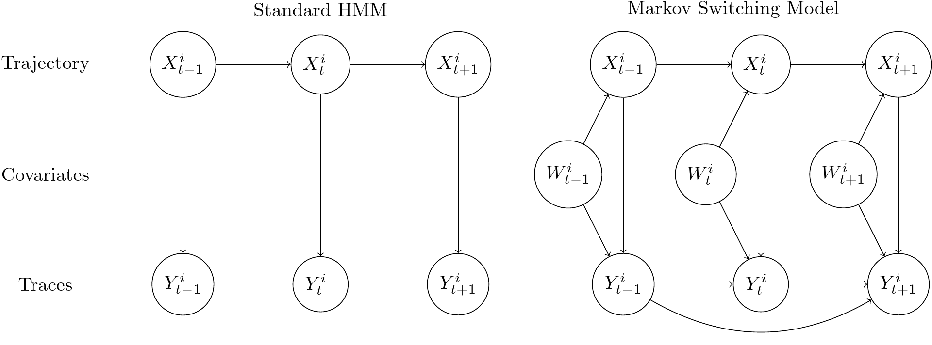
Figure 1: Comparison between standard HMM and Markov switching model.

3.2 Configuration for auto-regressive behaviors

The reader might wonder why it is necessary to allow for autoregressive behavior in the estimation of $\beta^{2}$ by including lagged values of $Y_{t}^{i}$ within $W_{t}^{i}$. First, some individuals might structurally leave more traces than others because they are in certain positions, for example, as service directors instead of regular high civil servants. This can be described as a hidden heterogeneity of the public sector that is not well captured by our very low-dimensional state space. Second, after observing a trace $Y_{i,t}=1$, it will often occur that $Y_{i,t+1}=1$ too, because an individual might have joined a temporary mission or committee. This could be seen as some sort of self-excitation behavior of the trace counting process. These problems of hidden heterogeneity and self-excitation can lead to a misspecification of the emission parameters that will then be propagated to the transition parameters $(\gamma_{0,t}^{i}),(\gamma_{1,t}^{i})$, and then the imputed trajectories $(X_{i,t})$.

We point out that, unlike most prior work using Markov switching models, the conditional distribution of $Y_{t}^{i}$, given $X_{t}^{i}$ is a Bernoulli distribution rather than a Gaussian distribution. This makes the usage of lagged values of $(Y_{t}^{i})$ in $W_{t}^{i}$ more difficult as implementing a causal gaussian autoregressive model AR(p) isn’t possible. Also, including all past values could lead to overfitting issues (as trajectories can be of length 60), and isn’t practical as it leads to having a covariate vector $W_{t}^{i}$ of varying size. In our model, we thus use a low-dimensional summary statistic of the past trajectory, which carries both long and short-term information, for hidden heterogeneity and self-excitation problems.

We provide short term information by including in $W_{i,t}$ a transformation of the time since the last trace was emitted for $i$

$$L_{t}^{i}=\sqrt{\max\{p\ |\ \forall s<p,Y_{t-s}=0\ \text{and}\ Y_{t-p}=1\}-1}.$$

For long-term information, we provide the average number of traces left by unit of time in the past trajectory

$$A_{t}^{i}(1)=\frac{\sum_{0<s\leq t}Y_{i,t-s}}{t}.$$

For medium-term information, and also to enable the model to pick up on changes of intensity, we provide a weighted average of the number of traces left in the past, which puts more emphasis on recent ones

$$A_{t}^{i}(\varphi)=\frac{\sum_{0<s\leq t}\varphi^{s}Y_{t-s}^{i}}{\sum_{0<s\leq t}\varphi^{s}}$$

with $0<\varphi\leq 1$ a weighting parameter. We empirically found that setting $\varphi=0.8$ produces satisfactory results.

Finally, this model needs to be robust to our sampling scheme, so as not to “sample on the dependent variable”. By definition, all individuals have a trace at the start of their span $T_{\text{min}}^{i}$, and so this should not be included in the estimation. In this process, we will not count this trace in the computation of $A_{t}^{i}(\varphi)$, by setting $Y_{i,0}=0$, and will treat early observations where this average equals 0 as a separate case. This is also why our derivation of the likelihood for $\beta^{2}$ only starts at $T_{\min}^{i}+1$. This yields the following 6-covariates vector

$$W_{2,t}^{i}=\begin{bmatrix}1\\ {L_{t}^{i}}\\ A_{t}^{i}(1)\\ A_{t}^{i}(0.8)\\ \mathbb{I}_{\left\{A_{t}^{i}(1)=0\right\}}\\ \mathbb{I}_{\left\{A_{t}^{i}(1)=0\right\}}L_{t}^{i}\end{bmatrix}$$

These 6 covariates give a succinct representation of the past trajectory. In the case, there exists a rigorous estimation of the age of the individual, there are better operationalizations interacting $1_{\left\{A_{t}^{i}(1)=0\right\}}$ and $L_{t}^{i}$.

3.3 Sampling strategy

We sample the posterior of the $(\beta^{k}),k=0,1,2$ via a Metropolis-within-Gibbs MCMC algorithm, following a Bayesian data augmentation scheme [Tanner and Wong, 1987]. Each iteration of our MCMC sampler includes two steps, described in detail below: (1) Gibbs sampling to draw unobserved $X_{t}^{i}$ points using all available information and parameters, and (2) update the $(\beta^{k})$’s using Metropolis-within-Gibbs steps.

3.3.1 Gibbs step for unobserved values of $X$

The Gibbs step consists of simulating missing values of $X_{t}^{i}$ given observed values of $X_{t}^{i}$, $Y_{t}^{i}$ and parameters $\beta^{k},k=0,1,2$. The transformed parameters $\gamma_{0,t}^{i}=\text{logit}^{-1}(W_{t}^{i}\beta^{0}),\gamma_{1,t}^{i}=\text{logit}^{-1}(W_{t}^{i}\beta^{1})$ and $\lambda_{t}^{i}=\text{logit}^{-1}(W_{t}^{i}\beta^{2})$ are computed using the Baum-Welch algorithm, which does not require the transition or emission parameters to be constant across time and units. Our implementation is strongly inspired by that of the R package HMM [Himmelmann, 2022].

We simulate all missing data points at each iteration. This might seem suboptimal, but since the Gibbs phase is not the driving cost of the algorithm, we do not attempt to further optimize this step.

3.3.2 Metropolis-within-Gibbs step for parameters

Our MCMC algorithm is inspired by the presentation of [Marin and Robert, 2014], which we apply successively to the three GLM settings for $\beta^{0},\beta^{1}$, and $\beta^{2}$. Each parameter vector $\beta^{k}$ is updated separately. For each $k$, we initialize by computing the MLE $\hat{\beta}^{k}$ and the covariance matrix $\hat{\Sigma}^{k}$ corresponding to the asymptotic covariance of $\beta^{k}$, and we set $\beta^{k}_{0}=\hat{\beta}^{k}$. We then run a subloop with $m=1,...,N_{\text{Metropolis}}$, and

1. Generate a proposal $\tilde{\beta}^{k}\sim\mathcal{N}(\beta^{k}_{(m-1)},\tau^{2}\hat{\Sigma}^{k})$, with $\tau$ a hyperparameter.

2. Compute

   $$\alpha(\beta^{k}_{(m-1)},\tilde{\beta})=\text{min}\left(1,\frac{\mathcal{L}(\tilde{\beta}^{k}|X_{i,t},Y_{i,t})}{\mathcal{L}(\beta^{k}_{(m-1)}|X_{i,t},Y_{i,t})}\right)$$

   where the likelihoods are the ones defined in Section 3.1.

3. Set

   $$\beta^{k}_{(m)}=\begin{cases}\tilde{\beta}^{k}&\text{ with probability }\alpha(\beta^{k}_{(m-1)},\tilde{\beta})\\ \beta^{k}_{m-1}&\text{ otherwise.}\end{cases}$$

The value $\beta^{k}_{N_{\text{Metropolis}}}$ is used as the output of the Metropolis-within-Gibbs step of one iteration. We set $\tau=1$ and $N_{\text{Metropolis}}=30$, which produces well-mixing sequences in our tests.

4 Study 1. ENA graduates and temporary exit

4.1 Motivation

As said earlier, former ENA students constitute a natural population when studying revolving doors, as they hold a central position in the organization of the French state. [Rouban, 2014] conducted a survey over 6 student promotions (n = 620) who graduated in 1969-1970, 1989-90, and 1999-2000. He reports that, 10 years after graduating, 8.3% of students from the first two cohorts were working in a private company, compared to 14.5% for the two next cohorts, and 9.5% for the last two, which indicates year-to-year variation but not a clear trend toward increasing exit rate to the private sector.

The results of [Rouban, 2014] seem to show that the average time taken for an ENA graduate before leaving the public sector has drastically decreased over time, which would imply a stark increase in the exit rate from the state, at least for young graduates. We must however note that the methodology of [Rouban, 2014] does not allow for comparing different cohorts for metrics that exhibit a dependency on the observation frame. Indeed, many statistics considered in that study are subject to right-censoring; this was not accounted for or acknowledged. It will lead to bias in all the estimates which are not robust to right censoring since the observation frames across cohorts significantly diverge: it was, at the time of publication, 44 years for the 1970 cohort, but only 14 years for the 2000 cohort. As individuals in the 2000 cohorts who would have left the public sector after more than 14 years simply could not be observed (as it had not yet happened), it is completely normal to observe a decrease in the average time taken before leaving. The results we present below on the 1990-2022 time period do not display a stark decrease in this indicator when the observation frame is taken into account. We assume the difference is due to our methodology properly taking into account the different lengths of observation frames. This leads us to conclude that the vast majority of this variation reported by [Rouban, 2014] is artefactual. Other quantitative conclusions of this work are not subject to this bias and are overall coherent with our results.

[Bouzidi et al., 2010] focus on a subgroup of ENA graduates, of the “civil administrator” status working in the Finance Ministry, between 1960 and 2002 ($n=438$), using hand-collected data. They show that, on their sample, about 40% of individuals went at least once into the private sector 20 years after graduating. The advantage of this approach is that they used a formal duration analysis model and are not susceptible to right-censoring biases. They however do not attempt to estimate whether there was an acceleration or not on their period of study, and stress that doing such inference is difficult for later cohorts because of right-censoring. They also estimate time spent in the private sector using simulations using two Weilbull distributions, one for the public sector and one for the private sector. Our work can be seen as a discretization of such a procedure, that enables missing data imputation and so to work with a majority of missing values, thanks to the formal framework of Hidden Markov models. Not discretizing while having missing values has a huge computational cost, as it isn’t possible to rely on closed-form forward-backward equations in the Gibbs step.

We build our first study from these surveys and provide two improvements (besides accounting for right-censoring effects for the first one). First, thanks to our methodology, we can broaden the scope and analyze all students who graduated between 1991 and 2021. In addition, since our modeling accounts for the fact that people can come back after leaving for the private sector, we can measure more precisely the public exit rate, and distinguish between individuals leaving permanently or not in the public sector.

4.2 Models

We implement four initial configurations which are, from simplest to most complex:

• Model 1 is a standard hidden Markov model, that is, for which we only include an intercept as a covariate within $W_{t}^{i,k},k=0,1,2$.

• Model 2 is a simple Markov switching model for which only the autocorrelation covariates described in the corresponding section are included for the estimation of $\lambda$.

• Model 3 adds a time-varying component depending on the age of individuals. Age is encoded as time elapsed since the person was admitted to ENA, on a range from 0 to 1 (with 1 corresponding to the entire time frame, 32 years). Age is modeled in a semi-parametric fashion, using B-splines of degree 2, with 5 degrees of freedom, and boundary knots in 0 and 1. We do this in order to saturate the model on the age dimension, so we can safely identify an effect related to cohort or period in later configurations. Using splines works better than multiple powers of age: under this parameterization, parameters are less correlated, so the sampler mixes faster. We include age coefficients for $\gamma_{0}$ and $\gamma_{1}$, but not for $\lambda$, as testing showed age was redundant and less effective than autocorrelation covariates, and would add instability in all estimates.

• Model 4 adds a cohort effect for the estimation of $\gamma_{0}$, $\gamma_{1}$ and $\lambda$. Cohort is encoded as the time at which the individual was admitted at ENA, ranging between 0 and 1 (the time at which it happened divided by the number of periods). As we also include saturated age-related coefficients, we can interpret the historical change essentially as an age-cohort decomposition (and specifically focus on the cohort aspect). To ensure this coefficient is not influenced by the duration of observation, we interact it with a dummy encoding the fact the individual isn’t in ENA anymore (that is, $F_{t}^{i}=1\ \text{for}\ t>T_{\text{min}}+4$). We choose to include time spent in ENA as some students immediately leave the public sector once they have finished school.

Models 1, 2, and 3 mainly serve as a baseline, as we are interested in the cohort coefficients to understand how revolving doors have evolved. We run our MCMC sampler on 5000 iterations and discard the first 200 as a burn-in period. Visual checks show that this is sufficient to guarantee convergence and the MCMC sampler mixes well. The Effective Sample Sizes of all parameters are above 200.

4.3 Results

4.3.1 Parameter posteriors

The simplicity of Models 1 and 2 enables full reporting on the posterior of their coefficients, which we do in Table 4 with their 0.05, 0.50 and 0.95 quantiles. Full information about coefficients for more complex models can be found in the digital appendix of this article, and we adopt a more summarized and graphical presentation. Figure 2 summarizes coefficient variation across time for $\gamma_{0}$ and $\gamma_{1}$ in Model 3.

Table 3: Coefficients for Models 1 and 2.

	$M_{1}$	$M_{1}$	$M_{1}$	$M_{2}$	$M_{2}$	$M_{2}$
quantile	q05	q50	q95	q05	q50	q95
$\gamma_{0}$, (Intercept)	-4.233	-4.171	-4.111	-4.621	-4.542	-4.465
$\gamma_{1}$, (Intercept)	-4.054	-3.938	-3.83	-3.667	-3.525	-3.391
$\lambda$, (Intercept)	-1.51	-1.492	-1.474	-1.853	-1.786	-1.718
$\lambda$, $L$				-0.16	-0.134	-0.108
$\lambda$, $A(1)$				-0.133	0.088	0.315
$\lambda$, $A(0.8)$				2.027	2.249	2.467
$\lambda$, $I(A(1)=0)$				0.102	0.191	0.279
$\lambda$, $I(A(1)=0):L$				-0.173	-0.137	-0.101

The main effect of adding autocorrelation coefficients from model 1 to model 2 can be observed in the difference between their median intercept for $\lambda$. For model 1, the median intercept is at $-1.492$ ($I_{90}=[-1.51,-1.474]$), which essentially corresponds to an average probability of 0.22 for an individual to generate a trace at any point in time. This is problematic as there are both high inter-personal and temporal variances. The median intercept for model 2 is lower, at $-1.786$ ($I_{90}=[-1.853,-1.718]$), more in line with what could be expected. All credible regions for autocorrelation coefficients except $A(1)$ do not contain zero and it can at least be assumed that they are not detrimental in estimating the local emission probabilities $\lambda_{t}^{i}$. In detail, we see that the coefficient for $L$ is negative, meaning that an individual who remained in the public sector for a few time points without emitting at least a trace has a lower probability of doing so, which covers the short-term property we mentioned. The coefficients for $A(1),A(0.8)$ are both positive ($\text{med}=0.088,I_{90}=[-0.133,0.315],\text{med}=2.249,I_{90}=[2.027,2.467]$), meaning that there is indeed a medium-to-long-term effect of trace generation on subsequent trace generations. As the two quantities are correlated, their credible intervals are larger, but this is not linked to a meaningful change to actual estimated probabilities $\lambda_{t}^{i}$ and data marginals $X_{t}^{i}$, and so the uncertainty is not communicated to other coefficients. Finally, the $\mathbb{I}_{A(1)=0}$ coefficient has an effect, with a negative coefficient. Let us add that this coefficient is, as wanted, the most dependent on the precise definition of the population: in conditions where we imposed less stringent criteria on the minimal number of emitted traces for someone to be included, this coefficient was the only one to significantly change.

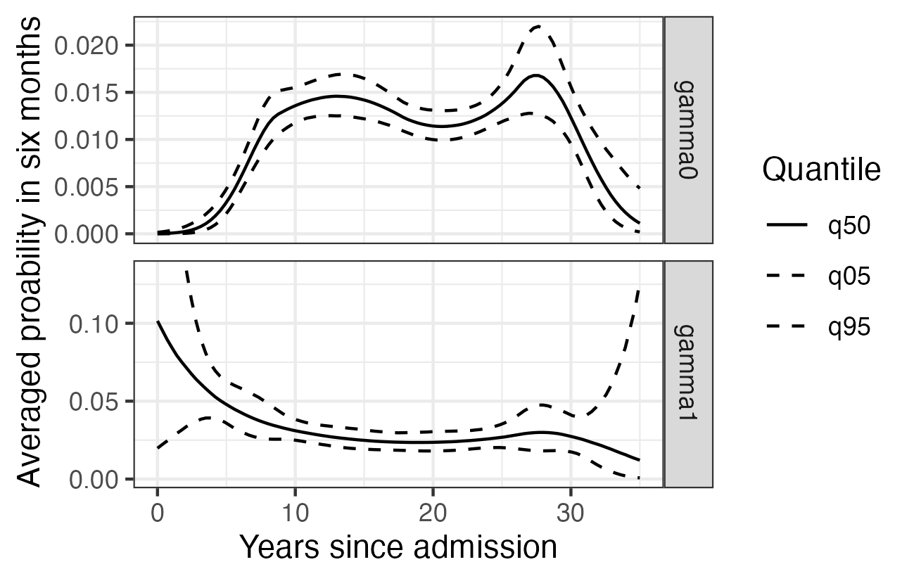
Figure 2: Median marginal probabilities across time given in Model 3

Figure 2 summarises information related to the probability of transitioning between states depending on age. It was computed by taking the inverse logistic transform of the sum of the intercept with the age spline coefficients. We first observe, that, around 0 years after admission, the probability of leaving for the private sector $\gamma_{0}$ is very low, as is expected by design since we didn’t keep individuals who immediately resigned from ENA or for whom no trace could ever be found beyond their admission after multiple years. The probability to come back $\gamma_{1}$ is very high, but note that this concerns a very slim (non-existent) proportion of the population. Median probability $\gamma_{0}$ then increases to $0.013$ where it remains more or less constant up to 25 years after admission. A stabilization occurs for $\gamma_{1}$ at around double the rate, at $0.025$. This is interesting as we observe there isn’t an important variation in the probability of leaving across the career, and the hypothesis of an overall geometric rate for leaving and coming back is quite realistic. There is a change of behavior 30 years after admission, but this is artefactual, as almost no one in the population has had the time to arrive at this stage (since our observation frame is 32 years long).

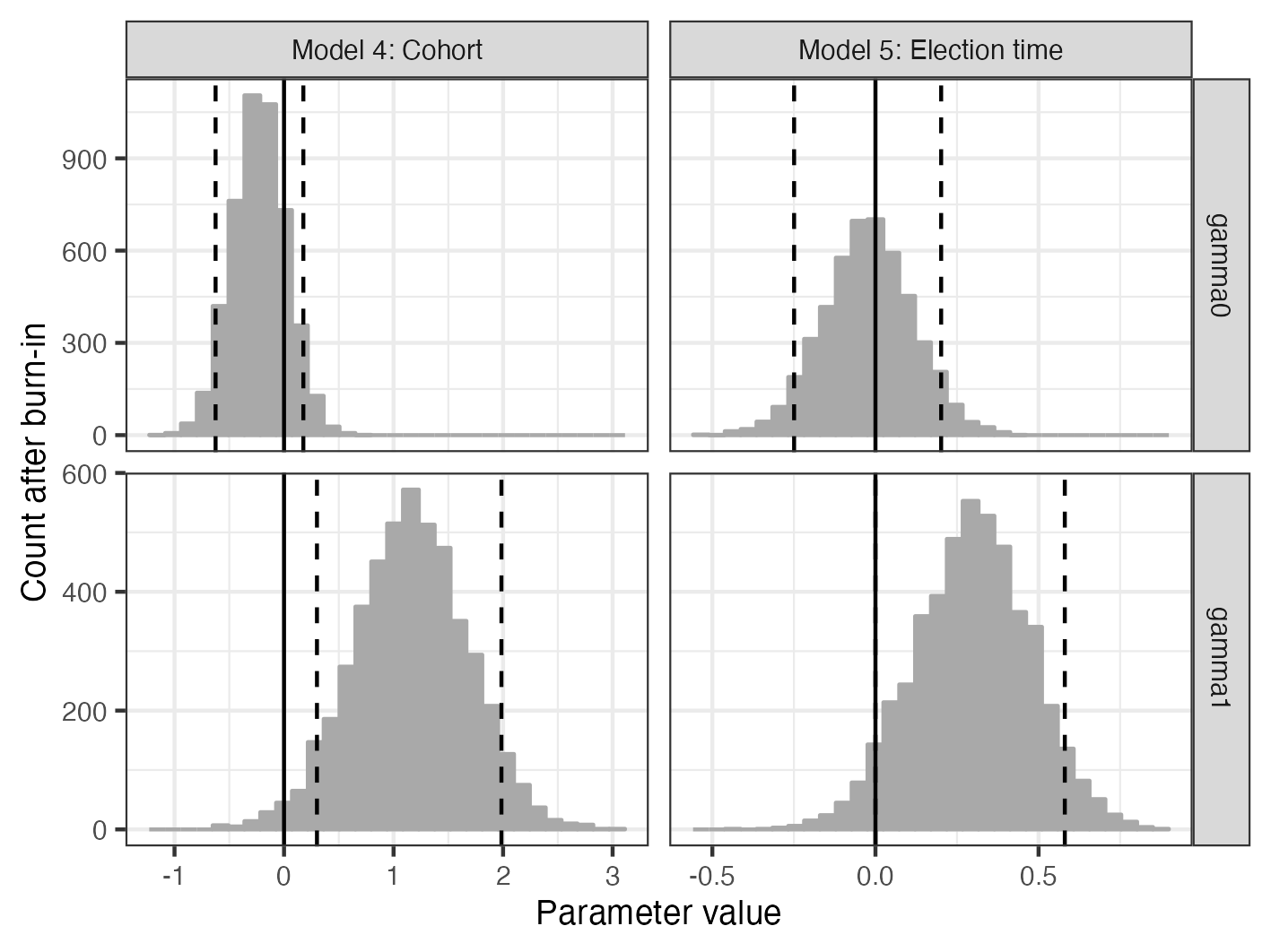
Figure 3: Posterior distribution of selected parameters for models 4 and 5. Left: effect of the cohort. Right: effect of the indicator that it is an election year. Top: Posterior of the parameter $\beta^{0}$ measuring the impact on the probability of leaving the public sector $\gamma_{0}$. Bottom: Posterior of the parameter $\beta^{1}$ measuring the impact on the probability of returning $\gamma_{1}$.

We can now turn to our main interest, cohort-related coefficients, which are presented in the left pane of Figure 3. The view is quite contrasted between $\gamma_{0}$ and $\gamma_{1}$. On the one hand, it isn’t possible to conclude that the chance of leaving for the private sector $\gamma_{0}$ has significantly changed across the period, as the credible interval well includes zero ($\text{med}=-0.226,I_{90}=[-0.625,0.176]$). However, it is at least possible to state strongly that this coefficient has not increased across time, and has quite possibly decreased. On the other hand, we can state with fair confidence that $\gamma_{1}$ has increased over time, with $\text{med}=1.16$, ($I_{90}=[0.301,1.98]$). These results are robust to misspecification, as shown by checks with modular inference described in Appendix B. We thus conclude that on the one hand, the probability of leaving the public sector has not increased in the period, and may even have decreased; and that the probability of coming back has increased in the period, contrary to what we expected before conducting this study.

4.3.2 Data posteriors and the suspicion for political dependence

Another, more descriptive way of analyzing results is to focus on observed and simulated data marginals $(X_{t}^{i})$ instead of parameter posteriors. In Figure 4, we report summaries for the probability of individuals to be in the private sector 12 years after being admitted into ENA (so 10 years after graduation), for admission years ranging from 1990 to 2010. We communicate the uncertainty of point values $X_{T_{\min}+23}^{i,n}$, which is larger than the uncertainty of expected values $\mathbb{E}[X_{T_{\min}+23}^{i,n}]$, and would decrease as a function of cohort size. As it is costly to store posteriors for all observation points at all iterations, this figure is only computed for the last 300 (without a big effect on precision).

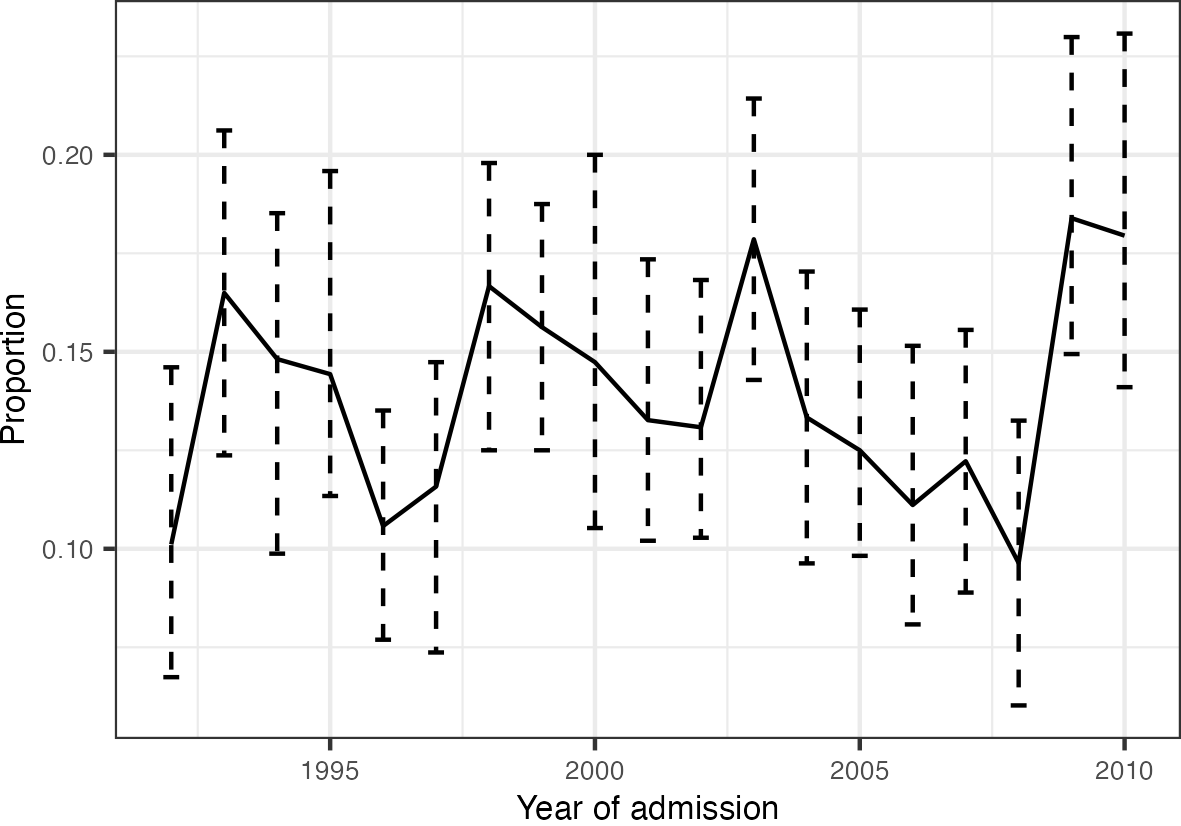
Figure 4: Inferred proportion of individuals not in administration 12 years after admission into ENA.

A first observation is that data posteriors confirm our analysis that, at least, the chance for leaving into the private sector has manifestly not increased in the period: we would otherwise observe an increase in the proportion of individuals not in administration. This absence of change is present even when including individuals who immediately leave the school before graduating. It is harder to make claims about $\gamma_{1}$ as we only describe individuals 10 years after graduating.

One could also observe a type of cyclical pattern that could, at first glance, be linked to changes in political majorities. For example, there are noticeable increases in cohort-year gaps 1991-1992, 1997-1998, 2007-2008, which could correspond to political shifts 10 years after, because of elections. However, the correspondence is not perfect and it could also be the product of other phenomena (or simply statistical variation due to small cohort sizes). To get a better sense of this, we implemented an additional model. Model 5 is similar to dichotomous Model 4, except for the fact that instead of a cohort effect, we estimate a period effect using a dummy variable:

$$P^{i}_{t}=\begin{cases}1&\text{if $t$ or $t+1$ is an election time point and $i$ has graduated}\\ 0&\text{else}\end{cases}$$

Election time points correspond to Jan-Jun 1995, 2002, 2007, 2012, 2017, 2022. This dummy is shifted by one unit (so $t+1$ or $t+2$) for $\lambda$. The posterior for the election time effects are reported in the right pane of Figure 3. We observe that the overall size of potential effects is far smaller than for period effects, and so should be interpreted cautiously. On the one hand, the conclusion for the absence of effect can be drawn for $\gamma_{0}$, as the credible interval is very well centered on zero ($\text{med}=-0.0212,I_{90}=[-0.249,0.201]$). On the other hand, however, despite important uncertainty, there seems to be a small positive effect of election time on $\gamma_{1}$ ($\text{med}=0.302,I_{90}=[0.000,0.302]$). In summary, electoral shifts probably do not influence the chance of high civil servants to leave for the private sector, but it seems to lead to higher chances of coming back for those who left.

4.4 Conclusion

We conclude that exit rates from the state have not increased on the period for former ENA students, contrary to what we expected before conducting this study. If a change was to be inferred from the data, it would rather be that elite civil servants have now a lower probability of leaving for the private sector than before, but it is possible to remain undecisive. Furthermore, the rate of former civil servants coming back to work in the public sector after leaving has significantly increased over the period. In other words, when civil servants leave for the private sector, they now have a higher chance of coming back. If there seems to be an interaction between political majority changes with election years and revolving doors for this population, it seems to affect the chance of coming back from the private sector than the probability of leaving.

These results also suggest why some more qualitative accounts would claim increased mobility between the public and private sectors for former ENA students. There is now a higher proportion of ENA graduates who have had experience in the private sector after graduating before coming back to work for the public sector. However, the claim that ENA students do not remain in the public sector anymore has to be significantly nuanced, and even rejected.

5 Study 2. Revolving doors across the state

5.1 Motivation

Different researchers have studied the trajectories of high civil servants and cabinet members in France by defining populations based on organizational belonging at a certain time point, especially by focusing on their past trajectory.

[Rouban, 2010] studied the finance general inspection (IGF) on the 1958-2008 period. IGF appears to have an important place in the revolving doors phenomenon, as they identified that over the 578 inspectors present in the organization between 1958-2009, a majority had wandered at least once in the private sector (62%). They identify a discontinuity around 1990, with a massification of individuals having done a business school before attending ENA and then IGF. They also observed after 2000 a growing proportion of IGF members who have had an experience in the private sector before coming back, which seems quite aligned with results obtained in our first study with a positive cohort effect for $\gamma_{1}$. However, we stress that the lack of use of any duration analysis model also probably leads here to biased estimates of quantities that are dependent on the observation time frame, either directly with the time spent in the private sector, or indirectly such as the position obtained when leaving for the private sector. The stark contrast of observation span between cohorts of this study (from 2 to 52 years) without proper acknowledgment of right-censoring effects casts doubt on affirmations such as the fact that these civil servants would not have access anymore to top direction positions from the private sector.

[Kolopp, 2021] conducted a study on the general direction of the treasury (DGtresor) in the 1965-2010 period. They exhibited a gendered behavior: men are more likely than women to leave for the most prestigious private industries (especially banking); on the other hand, they do not seem to show gender differences in the overall probability of leaving the public sector. They describe that differentiated practices generate unequal outcomes at different points in careers, for example with the stress on international mobility for career advancement and differences in professional networks. If we have reasons to assume these factors also play a significant role for other organizations, their strength may vary, and other factors might come into play. Even if we don’t differentiate within private sector activities, we will compare behavior between men and women across the different organizations of our sample.

In a slight shift of focus, [Dudouet and Grémont, 2007] studied business leaders of the 40 French companies with the highest financial market valuation. In their population, 28% of business leaders were former high civil servants. Among these 178 leaders with a background in the public sector, 38% were members of technical groups (Mines, Ponts, Télécoms (not covered here as identifying which ones have the right status cannot be done solely using our source), and 31% were members of General Inspection of Finances, Conseil d’État or Cour des comptes. Of course, the affirmation that many business leaders are from these organizations is different from the one we are studying, that is, the rate of exit from these organizations to the private sector.

We attempt to build upon their results and propose a complete and systematic comparison across the different organizations we mentioned. This has value in the sense that it can qualify statements regarding the most prestigious organizations that are represented in these studies: are they really that special compared to other powerful services? For example, are the Finance Inspection and Treasury that much more affected by revolving doors compared to other services in the economy ministry or other inspections? We can also test statements linked to individual properties: do men have higher chances to leave for the private sector, and then come back? We also test the specificity of former ENA students compared to other high civil servants: how much more do they participate in the revolving doors phenomenon?

Table 4: Proportion of men and ENA graduates by organization.

group	prop_men	prop_ena	group	prop_men	prop_ena
cprefet	87.6	11.7	dgfip	72.4	11.8
cdiplo	82.7	8.4	iga	71.4	31.0
dgtresor	80.7	26.3	ce	66.3	34.5
ccomptes	78.2	31.3	insee	64.8	0.3
igf	75.8	37.8	igas	61.5	29.8

5.2 Models

We encode organizational membership using a set of $D$ dichotomous variables $M_{t,1}^{i},...,M_{t,D}^{i}$ corresponding to our $D=11$ selected organizations, that we will include in the covariate matrices $W_{t}^{i}$. Contrary to the first study, we need to account for the fact that individuals can be affiliated to multiple organizations during their professional career. To remain consistent with our choice to focus on the main organizational identity of individuals, we impose that someone, at any given time, may only be linked to one organization in our set of $D$ organizations. This means we impose $\sum_{d=1}^{D}M_{t,d}^{i}=1$. If an individual is observed to become part of organization $d_{1}$ at time $t_{1}$ and then of organization $d_{2}$ at time $t_{2}$, we will have $M_{t,{d_{1}}}=1$ for $t_{1}\leq t<t_{2}$, and $M_{t,d_{2}}=1$ for $t\geq t_{2}$. This is a simplification, which has the advantage of enabling an analysis that is closest to what we could obtain by performing completely separate analyses for the different public organizations, even if it could be altered to study how having been the member of a given organization can affect behavior once being a member of another one included in the study.

We implement three configurations, from the simplest to the most complex:

• Model 1 is a Markov switching model for which we only include an interecept for each group, in addition to the autoregressive covariates for traces. The autoregressive covariates are interacted with the dummy of every organization. This is our reference model.

• Model 2 adds to the reference model a dichotomous variable encoding gender ($G_{t}^{i}=1\ \forall t$ if $i$ is a woman), for both $\gamma_{0},\gamma_{1}$ and $\lambda$.

• Model 3 aims at comparing, for every organization, former ENA students and non-former ENA students. It adds to the reference model a dichotomous variable encoding whether the individual was observed as being admitted to ENA at an earlier time point ($E_{t}^{i}=1\ \forall t$ if that is the case). This dichotomous variable is interacted with each organization for each organization dummy for $\gamma_{0}$ and $\lambda$, but not for $\gamma_{1}$ as it suffered from convergence issues as we did not observe enough cases for small organizations.

Observe that Model 3 has an implicit dependency on age, as information on having been an ENA student is censored if the individual was admitted before 1990 as we infer this information from the same archive, which could lead to biased estimates. To avoid that, we choose to remove individuals for which their first trace was found between 1990 and 1993. This has the cost of removing ENA students who had a career in the public sector before integrating the school between 1990 and 1992, and overall to exclude older individuals from the sample. The intercept of these models will thus naturally deviate from models 1 and 2, but we are here interested in the temporal and individual comparison, and will thus focus on these contrasts.

5.3 Results

5.3.1 Comparison across organizations

We report the $5,50,$ and $95$ quantiles of the posterior for each of these models. Median estimates of coefficients for Model 1 are reported in Figure 5, alongside their 90% credible interval, expressed in raw probability. Bear in mind that these are average coefficients that do not correspond to local probabilities individuals may have to leave at any given point in time, which are modulated by the observed traces and the local $\lambda$’s. As coefficients for DGfip stand out from the rest in both estimate and uncertainty ($\gamma_{0}\approx 0$), we do not report them in the Figure but do so in the text below.

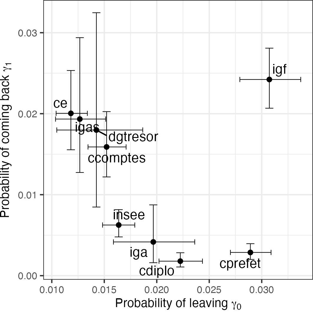
Figure 5: Coefficients for Model 1 expressed in probabilities.

We can firstly observe and rank organizations depending on the chance individuals have to leave for the private sector when they are part of them. On the side of organizations with the highest departure rate, we find the General Inspection of Finances ($p_{\text{IGF}}=0.031$) and Prefects group($p_{\text{Cprefet}}=0.029$). In an intermediary situation, we find the Diplomats group ($p_{\text{Cdiplo}}=0.022$), the General Inspection of Administration ($p_{\text{IGA}}=0.020$), the statistical office ($p_{\text{Insee}}=0.016$). At the lower hand of the spectrum, we find Cour des Comptes ($p_{\text{Ccomptes}}=0.015$), Treasury ($p_{\text{DGTresor}}=0.014$)), the General Inspection for Social Affairs ($p_{\text{Igas}}=0.013$), and the Conseil d’État ($p_{\text{CE}}=0.011$). Not shown in the table, the General Direction for Public Finances has the lowest probability ($p_{\text{DGfip}}=0.006,I_{90}=[0.004,0.009]$). This last very low coefficient means that there are almost no departures from this direction, and when that is the case, civil servants move first to another service included in this study. The overall ranking should be intuitive to the reader accustomed to the question – the model rightly identifies that individuals in the Treasury have a higher chance of leaving for the private sector than individuals in the Inspection for Social Affairs. A seemingly counterintuitive result is the position of IGF and CComptes: these two groups have a similar function (financial auditing of the state), but have very different positions in Figure 5; this observation is in fact aligned with an effect identified in the survey from [Charle, 1987].

We observe interesting contrasts in the chance of individuals to come back working in public administration after being in the private sector. Inspection of Finances again clearly stand out, with ($p_{\text{IGF}}=0.024$). With varying levels of uncertainty, Conseil d’État ($p_{\text{CE}}=0.020$), Inspection of social affairs ($p_{\text{IGAS}}=0.019$), Treasury ($p_{\text{DGtresor}}=0.018$), and Cour des comptes ($p_{\text{DGtresor}}=0.016$), they appear in an intermediate situation. At the lower end of the spectrum, we observe the statistical office ($p_{\text{Insee}}=0.006$), inspection of administration ($p_{\text{IGA}}=0.004$), prefects ($p_{\text{Cprefets}}=0.003$), and diplomats ($p_{\text{Insee}}=0.002$).

We thus conclude that the two rankings are not convergent and would even be negatively correlated if we excluded IGF. However, we find it more accurate to describe this as forming three groups. First, IGF constitutes a group on its own, standing out from the rest as having both high probabilities for leaving and coming back. Classical results claiming that moving into the private sector is part of the career advancement process hold well, and we further prove that this is quite distinctive to this organization. We identify a second group of organizations where the chance of leaving is relatively high, but the chance of coming back is rather low: this concerns the statistical office, the inspection of administration, diplomats and préfets. The situation is unsurprising for the first two, which are known to be closer to the private sector than other organizations. For préfets and diplomats, this might be because we study individuals who are simultaneously at the top of certain services but without as high position security as in other organizations (such as Conseil d’État, where people can keep their status): people (involuntarily) leaving could find themselves unable to come back. Finally, we find a group of organizations where the chance to leave is comparatively low and the chance to come back high: Conseil d’État, Inspection of Social Affairs, Cour des Comptes. One could also place Treasury in this group, but parameter uncertainty (especially on $\gamma_{1}$) requires caution. This concerns organizations for which members acquire life-long status that can help them come back after leaving; and also for which clear career advancement schemes exist in the public sector.

5.3.2 Interaction with gender and status

The posterior of the odds ratio for women versus men and ENA graduates versus other high civil servants can be found in Figure 6 as a way to summarise interest parameters for models 2 and 3. A distribution on the right means we have grounds to think the alternative group (women/ena-students) has a higher chance of leaving for the private sector than the reference group, and vice-versa. A distribution centered on 1 indicates we should remain indecisive on the matter.

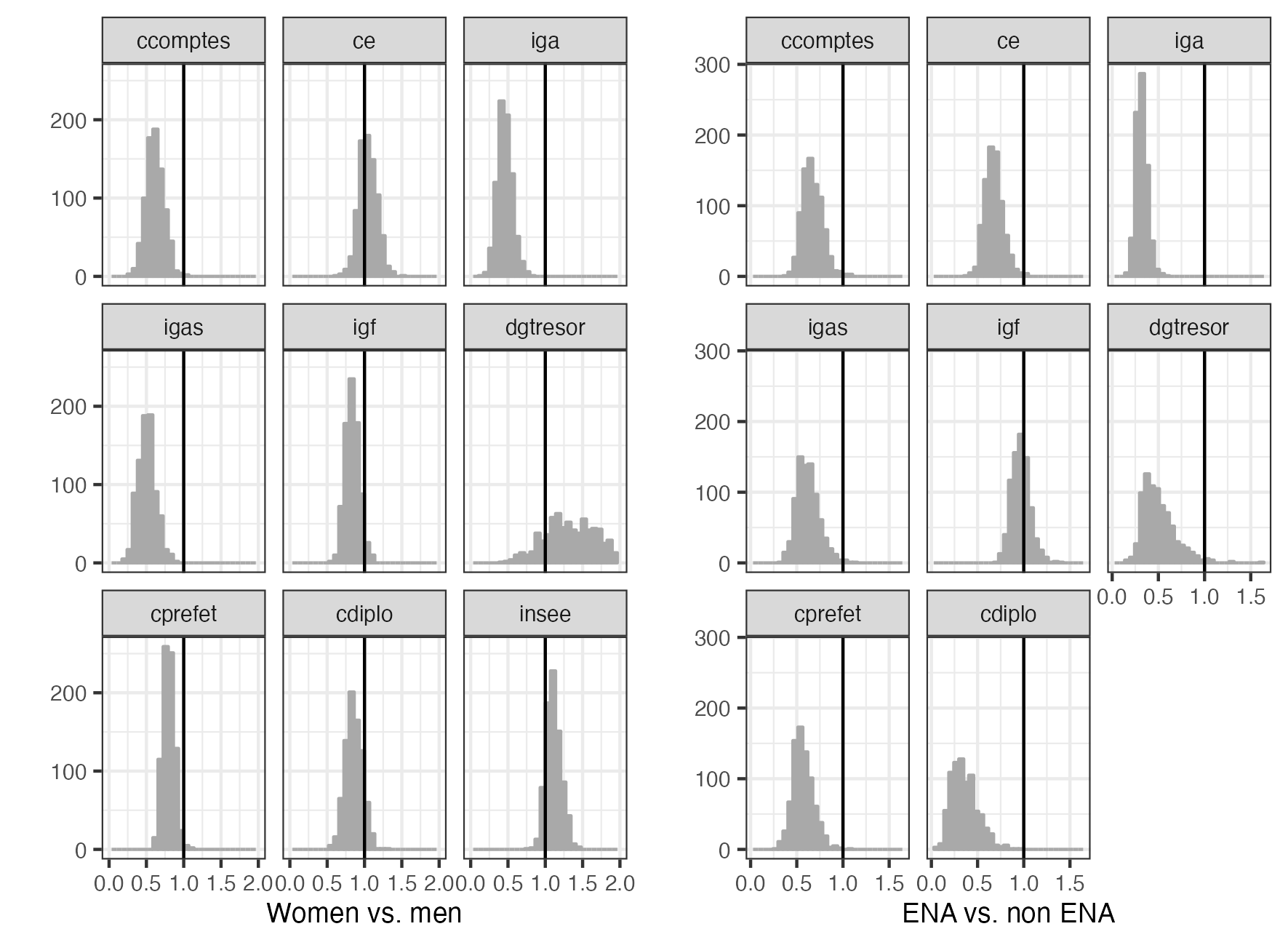
Figure 6: Odds-ratios for models 2 and 3.

Not all organizations have the same profile of differentiated practices between men and women, but a broad conclusion can nonetheless be inferred: women have less chance than men to leave for the private sector. For certain organizations, the difference is strong and identifiable: Cour des Comptes, Inspection of Administration, Inspection of Social Affairs (odds ratios below 0.7). The difference is smaller but still observable for Inspection of Finances, Préfets, and Diplomats. The situation is undecided for Conseil État and the Statistical Office, the latter suggesting a small positive effect on the side of women. Treasury here stands out in terms of uncertainty (as there are less than 200 individuals to work on and a small proportion of women), but the side of the effect would be rather positive for women.

Somewhat unexpectedly, individuals who have graduated from ENA tend to wander less into the private sector than others. We find this counter-intuitive in the sense that our population-definition scheme is rather strict, only keeping high-status positions. So even if individuals in the highest position of power tend to wander more into the private sector, being an ENA student doesn’t increase further the probability of leaving the private sector. On the other hand, as ENA graduates still access these high-status positions more, on a purely descriptive level, they could still be found to more often go to the private sector than other civil servants. We can interpret this fact for rather unstable positions such as Prefects and ambassadors: ENA students are enable to better secure their position than their counterparts, and as a result, probably do not suffer from unwanted departures into the private sector. The difference is stronger for Inspection of Administration than for Cour des Comptes and Conseil d’État, and then Inspection of social affairs. On the other hand, the difference between the two subgroups is rather small for IGF, where it also stands out from other public organizations.

5.4 Discussion

This section reveals that Markov switching models enable the proper testing of substantive research hypotheses, at the intersection between organizational and individual effects. We find three profiles of organizations depending on the chance of leaving and the chance of coming back: one with high chances of leaving but low chances of coming back; one with low chances of leaving but high chances of coming back; and Inspection of Finances standing out from the rest with high chances of both to leave and to come back. Women have overall less chance to leave for the private sector than men, but the situation is not constant across public organizations. Finally, ENA graduates have less chance to leave for the private sector than their colleagues in this very elite portion of the public sector, except again for Inspection of Finances where the chance is constant across the board.

6 Overall discussion

Binary Markov switching models constitute a powerful and flexible tool that can be fruitfully used to analyze individual trajectory data with a large number of missing values. They explicitly model both the underlying trajectory behavior and the trace-emission process, which enables robust inference and has the interest of emulating a credible data-generating process. They can be well estimated using a custom MCMC sampler combining a Gibbs step and a Metropolis-within-Gibbs step. Only using traces from an administrative source with some supervision given by data from a digital platform, we can test substantive research hypotheses regarding how revolving doors are heterogeneous across time and organizations. It is not required to observe everything about everyone to draw substantive conclusions about collective behavior such as revolving doors.

We have shown that the rate at which ENA graduates exit the State has not increased for more recent cohorts since 1990, and that the rate of coming back working for the State after working in the private sector has significantly increased. A natural extension would be to consider individuals who were admitted before 1990, circumventing the fact that Journal Officiel was not easily accessible before that time frame and that it is harder to find digital profiles to facilitate learning. The cutoff of 1990 is more strict than what one could think, as it concerns the admission year and so excludes more senior ENA graduates who were admitted before but had a career after 1990 in study 1. In addition, we have identified three organizational mobility profiles, separating organizations for which rates of exiting are comparatively high but chances of coming back low (like INSEE); organizations with the reverse observation (like Conseil d’État); and a clear outlier found in the General Inspection of Finances. We observed that the exit rate for women is generally lower than for men, but that the situation is heterogeneous across organizations. Finally, we observed that, for our very selective civil servants population, being an ENA graduate is associated with a lower chance of exiting into the private sector.

A natural concern with using these models on such data is time heterogeneity: younger generations are more likely to have a digital profile account and this could bias inference. Two pieces of evidence seem to show we are robust to such misspecification: first, tests with modular inference which essentially gives null weight to individuals without a digital profile provide similar results; second, comparisons between models with and without time covariates give similar estimates for coefficients that are shared across the two models. However, these models still require more theoretical exploration to know precisely in which context they could lead to biased estimates.

An innovation in this paper is found in the way data was collected and cleaned. Our philosophy was to automate as much work as possible, for example in the name-matching phase, which enabled us to study a population an order of magnitude larger than what is usually done in traditional elite research (prosopography studies rarely exceed a few hundred individuals). However, we were not able to automate everything away, like public-private organization name classification, and the main limitation would again become human time if a researcher attempted to scale up this work by another order of magnitude. Our MCMC sampling procedure is, compared to approximate calculations, more costly, which could also be a problem when trying to scale up this approach. We found that the main cost of the procedure was in the computation of the MLE in the initialization of each Metropolis step, in addition to the random walk which required multiple computations of the likelihood. The cost of the Gibbs step was less important as it was very easy to parallelize it across individuals. Enabling a better scaling of the procedure could enable to study of a larger population, at a finer scale than based on six-month increments.

Finally, many other statistical developments could contribute to the study of elite literature. Our approach was simplified by the fact we only studied two states: public and private. However, many examples exhibit more complex (and continuous) state spaces, which could benefit for example from recent developments in (bayesian) machine learning sequence modeling. It remains to be seen, however, if more complex models could still enable the simple testing of substantive research hypotheses from the literature.

Appendix A Data assemblage

All traces and LinkedIn profiles are attached to a full name. There is therefore a high risk of the data being tarnished by homonyms. In this section, we describe the careful procedure used to eliminate this risk as much as possible, while preserving information.

A.1 Selection of administrative traces

For every person in our population, we query the Journal officiel to obtain every administrative order carrying the same name, which yields a first set of traces we name $S_{1}$. As many people have perfect homonyms, we have to filter this set. Most traces are tagged with one or multiple organizations, which range from small bureaus to the entire police force. To reduce this risk of perfect homonyms, we only keep traces linked to organizations significantly over-represented in $S_{1}$ compared to the entire Journal officiel. For each organization with the set $O$ of traces linked to it, we compute:

$$\frac{\mathbb{P}[O|S_{1}]}{\mathbb{P}[O]}=\frac{\#\{\text{traces linked to org}\ O\}\cap S_{1}}{\sum_{x}\#\{\text{traces linked to org}\ x\}\cap S_{1}}/\frac{\#\{\text{traces linked to org}\ O\}}{\sum_{x}\#\{\text{traces linked to org}\ x\}}$$

which can be interpreted as a relative risk score. We only keep traces linked to organizations with a score above 2, or above 1 if they have fewer than 1000 traces, or above 0.5 if they have fewer than 100 traces. This effectively removes organizations such as the army or the police where many promotions are described for the entire force, and constitute the main sources of perfect homonyms in $S_{1}$. For traces that are not linked to any organization, we also include them if they are a “délégation de signature” (meaning an authority delegates administrative power to the civil servant, a practice that remains limited in scope) or if it states an admission into a “grand corps”. This enables a good tradeoff between minimizing the homonymy risk and keeping as much data as possible, and yields a second set of traces $S_{2}$. For the first population, we then manually search for every individual for which we cannot find any trace upon graduation, and document the cases of name-changing for individuals who got married during their time as students (around 200 individuals) and add the relevant traces to the total after filtering them using the same procedure. For the second population, if a trace in $S_{2}$ documents the person has had another name, we also add the relevant traces after passing them through the same filters as before (this also represented around 200 individuals). This yields our final set of traces $S_{3}$.

A.2 Linkage with digital profiles

For each person in our population, we search on LinkedIn for up to three profiles that share the same name, download them, and then only keep the ones that list an experience in our starting set of organizations. For example, if an individual is included because they are part of the Statistical office, we only keep profiles with such an affiliation, using a rule-based approach. When more than one profile qualifies, we score the candidate profiles based on their affiliations and only keep the one with the highest score. Overall, we designed our scheme to minimize false matchings between sources rather than maximizing the number of profiles that would be matched; manual inspection shows that it is very robust to homonymy problems in the matching between the two sources. The proportion of individuals that could be matched with a digital profile for subgroups can be found in Table 3.

Table 5: Proportion of individuals by group with a matched profile.

group	prop	group	prop
ena	55.2	ce	37.9
dgtresor	54.4	insee	33.2
igf	52.3	dgfip	32.4
igas	44.5	cdiplo	26.8
ccomptes	41.5	cprefet	24.7
iga	37.9

For each profile linked to an individual, we obtain a list of dated professional positions that are shared between the public and private sectors (or “spheres”, see [Daho and Gally, 2018, France and Vauchez, 2017]). We classify organization names between public and private positions, using a rule-based method, progressively adding filters to capture all public organizations. This strategy enabled us to cover manually the entire sample. Companies entirely owned by the state (e.g. La Poste, France Television) are also coded as public, alongside companies with the “EPIC” status (e.g. SNCF, OSEO). Contrary to [Daho and Gally, 2018], companies that only have the state as a minority shareholder (e.g. Renault, TotalEnergies) are coded as private. In addition, positions at Universities and research bodies are not coded as either public or private: it appears they correspond to associate teaching positions that do not constitute the main occupation for people in our population, and so we leave them out. This reasoning leads us to also not code implication in a political campaign, as this is often superposed to other engagements. The same goes for positions in associations, naturally including charities, but also positions in unions, which include corporate representation bodies such as Medef. Finally, to ensure homogeneity with Journal Officiel, we do not include positions in world organizations (e.g. World Health Organization). This strategy of not coding uncertain cases is enabled by our modeling approach, as it doesn’t require full trajectories, and reduces the impact of such decisions on results. Without claiming this coding scheme is perfect, these decisions only have a minor impact on the substantial research findings, and all 1488 coding filters will be made fully accessible in the appendix for re-use.

A.3 Exact perimeter for organizational belonging

Readers interested in the functioning of the French "Grands Corps" will probably be interested in our precise definition of traces that define membership in any of them. Our definition is built in an empirical manner even if there are two defining principles. On the one hand, the definition is heavily constrained by the nature of the archive and what it documents, and on the other hand, it is based on a continuous discussion with sociologists and political scientists so the criterion adopted here would match usual accounts, and avoid being overly broad or narrow.

Concretely, we begin by surveying the Steinertriples API for the different groups we are interested in. We first filter out traces depending on the organization and their nature, using a rule-based approach summarized in the table (0 meaning we filter out). This was defined by discussing with field experts with concrete examples of the different cases.

Table 6: Type of traces used to define membership by organization

short_name	affectation	nomination	intégration	titularisation
cab	0	1	0	0
ccomptes	1	1	1	0
cdiplo	0	1	0	0
ce	1	1	0	1
cprefet	0	1	0	1
csprefet	0	1	0	1
dgbudget	1	1	1	1
dgfip	1	1	1	1
dgtresor	1	1	1	1
ena	0	1	0	0
iga	1	1	1	1
igas	1	1	1	1
igf	1	1	1	1
insee	0	1	0	0

After this first filter, we apply specialized regex filters to precisely filter the population so it resembles as much as possible expert interpretations.

• For CComptes, traces that are not affectation, we only keep matches of (auditeur)|(auditrice)|(conseiller)|(conseillère)|(président)|(magistrat). We include the array of elite civil servants working at the Court.

• For INSEE, we only keep traces that match (administrat)|(inspect)|(direct) and do not match (regiss)|(élève). We thus focus on members of the legal INSEE grand corps.

• For CE, traces that are not affectation, we only keep traces matching (auditeur)|(auditrice)|(conseiller)|(conseillère)|(maître). We focus on Conseillers d’États and auditors.

• IGAS, IGA, IGF, for nomination traces, we only keep matches of (inspecteur) |(inspectrice). We thus focus on inspectors.

• For DGtresor and DGfip, nomination traces, we only keep matches of (directeur) |(directrice)|(chef)|(administrat)|(délégué)|(attaché)|(conseiller). We also remove nomination traces matching (commission)|(expert)|(régisseur)| (suppléant). For DGfip, we also remove traces that document being a member of a cabinet. We thus mostly focus on directors and sub-directors of services and economics experts.

• For ENA, we only keep traces of admitted students.

After applying this filter, we then remove nomination traces matching (membre) |(représentant) which correspond to internal elections.

Appendix B Data heterogeneity concerns and modular inference

In our inference procedure, we use both values of $(X_{t}^{i})$ which have been observed (on LinkedIn), and values which have been simulated from the appropriate conditional; both types of values will be used to infer the parameters of interest. As our two data sources are of very different nature, the heterogeneity it may create can be disquieting. Even in the slightest misspecification case, simulated data could be a lot less trustworthy than observed data, and errors on the former could be propagated to the entire estimation procedure. In addition, even if we attempted to classify the digital data so it would match as best as possible administrative accounts, some residual artefactual differences could still be observed.

This problem of having multiple, heterogeneous data modules is common and has been discussed in the Bayesian literature [Jacob et al., 2017]. For each configuration, we consider two settings: (a) all values are treated equally; (b) simulated values are given a weight of 0.01, whereas observed values are given a weight of 1. This second strategy effectively grants all importance to individuals who have a digital profile.

Simulations in modular inference control condition leads to a similar conclusion on $\gamma_{1}$, with a posterior on $\gamma_{0}$ a little more shifted to the negative side.

References

- [Bienen and Van de Walle, 1991] Bienen, H. and Van de Walle, N. (1991). Of time and power: Leadership duration in the modern world. Stanford University Press.
- [Bouzidi et al., 2010] Bouzidi, B., Gary-Bobo, R., Kamionka, T., and Prieto, A. (2010). Le pantouflage des énarques : une première analyse statistique. Revue française d’économie, XXV(3):115.
- [Box-Steffensmeier et al., 2007] Box-Steffensmeier, J. M., De Boef, S., and Joyce, K. A. (2007). Event Dependence and Heterogeneity in Duration Models: The Conditional Frailty Model. Political Analysis, 15(3):237–256.
- [Charle, 1987] Charle, C. (1987). Le pantouflage en France (vers 1880-vers 1980). Annales. Histoire, Sciences Sociales, 42(5):1115–1137. MAG ID: 2076063633.
- [Daho and Gally, 2018] Daho, G. and Gally, N. (2018). Le cabinet ministériel comme espace frontière. Les collaborateurs ministériels passés par la sphère privée sous la présidence de François Hollande. Revue francaise d’administration publique, 168(4):849–874. Bibliographie_available: 1 Cairndomain: www.cairn.info Cite Par_available: 1 Publisher: Institut national du service public.
- [Dudouet and Grémont, 2007] Dudouet, F.-X. and Grémont, E. (2007). Les grands patrons et l’Etat en France: 1981-2007. Sociétés contemporaines, n° 68(4):105–131.
- [Fleischer, 2016] Fleischer, J. (2016). Partisan and professional control: Predictors of bureaucratic tenure in Germany. Acta Politica, 51(4):433–450.
- [France and Vauchez, 2017] France, P. and Vauchez, A. (2017). Sphère publique, intérêts privés. Enquête sur un grand brouillage. Sciences Po (Les Presses de).
- [Himmelmann, 2022] Himmelmann, L. (2022). HMM: Hidden Markov Models. R package version 1.0.1.
- [Jacob et al., 2017] Jacob, P. E., Murray, L. M., Holmes, C. C., and Robert, C. P. (2017). Better together? Statistical learning in models made of modules. arXiv:1708.08719 [stat].
- [Jäckle and Kerby, 2018] Jäckle, S. and Kerby, M. (2018). Temporal Methods in Political Elite Studies. In Best, H. and Higley, J., editors, The Palgrave Handbook of Political Elites, pages 115–133. Palgrave Macmillan UK, London.
- [King et al., 1990] King, G., Alt, J. E., Burns, N. E., and Laver, M. (1990). A unified model of cabinet dissolution in parliamentary democracies. American Journal of Political Science, pages 846–871. Publisher: JSTOR.
- [Kolopp, 2021] Kolopp, S. (2021). Pantoufler, une affaire d’hommes ?: Les énarques, l’administration financière et la banque (1965-2000). Sociétés contemporaines, N° 120(4):71–98.
- [Langrock et al., 2017] Langrock, R., Kneib, T., Glennie, R., and Michelot, T. (2017). Markov-switching generalized additive models. Statistics and Computing, 27(1):259–270.
- [Marin and Robert, 2014] Marin, J.-M. and Robert, C. P. (2014). Bayesian essentials with R, volume 48. Springer.
- [Meligkotsidou and Dellaportas, 2011] Meligkotsidou, L. and Dellaportas, P. (2011). Forecasting with non-homogeneous hidden Markov models. Statistics and Computing, 21(3):439–449.
- [Michelot, 2023] Michelot, T. (2023). hmmTMB: Hidden Markov models with flexible covariate effects in R. arXiv:2211.14139 [stat].
- [Rouban, 2010] Rouban, L. (2010). L’inspection générale des Finances, 1958-2008 : pantouflage et renouveau des stratégies élitaires. Sociologies pratiques, 21(2):19.
- [Rouban, 2014] Rouban, L. (2014). La norme et l’institution : les mutations professionnelles des énarques de 1970 a 2010. Revue française d’administration publique, 151-152(3):719.
- [Sandri et al., 2020] Sandri, M., Zuccolotto, P., and Manisera, M. (2020). Markov switching modelling of shooting performance variability and teammate interactions in basketball. Journal of the Royal Statistical Society Series C: Applied Statistics, 69(5):1337–1356. Publisher: Oxford University Press.
- [Tanner and Wong, 1987] Tanner, M. A. and Wong, W. H. (1987). The Calculation of Posterior Distributions by Data Augmentation. Journal of the American Statistical Association, 82(398):528–540. Publisher: Taylor & Francis _eprint: https://www.tandfonline.com/doi/pdf/10.1080/01621459.1987.10478458.
- [Wang and Puterman, 1999] Wang, P. and Puterman, M. L. (1999). Markov Poisson regression models for discrete time series. Part 1: Methodology. Journal of Applied Statistics, 26(7):855–869.
- [Wong, 2001] Wong, C. S. (2001). On a logistic mixture autoregressive model. Biometrika, 88(3):833–846.