SpliceMix: A Cross-scale and Semantic Blending Augmentation Strategy for Multi-label Image Classification

Abstract

Recently, Mix-style data augmentation methods (e.g., Mixup and CutMix) have shown promising performance in various visual tasks. However, these methods are primarily designed for single-label images, ignoring the considerable discrepancies between single- and multi-label images, i.e., a multi-label image involves multiple co-occurred categories and fickle object scales. On the other hand, previous multi-label image classification (MLIC) methods tend to design elaborate models, bringing expensive computation. In this paper, we introduce a simple but effective augmentation strategy for multi-label image classification, namely SpliceMix. The “splice” in our method is two-fold: 1) Each mixed image is a splice of several downsampled images in the form of a grid, where the semantics of images attending to mixing are blended without object deficiencies for alleviating co-occurred bias; 2) We splice mixed images and the original mini-batch to form a new SpliceMixed mini-batch, which allows an image with different scales to contribute to training together. Furthermore, such splice in our SpliceMixed mini-batch enables interactions between mixed images and original regular images. We also offer a simple and non-parametric extension based on consistency learning (SpliceMix-CL) to show the flexible extensibility of our SpliceMix. Extensive experiments on various tasks demonstrate that only using SpliceMix with a baseline model (e.g., ResNet) achieves better performance than state-of-the-art methods. Moreover, the generalizability of our SpliceMix is further validated by the improvements in current MLIC methods when married with our SpliceMix. The code is available at https://github.com/zuiran/SpliceMix.

I Introduction

As a fundamental task of computer vision, image classification (especially with single-label) has been well-studied from various aspects, such as network architectures [1, 2], data augmentation strategies [3, 4], and pre-trained models [5, 6]. However, some methods designed for single-label images are not always adaptive to the multi-label image classification (MLIC) task since a multi-label image usually contains multiple categories, which means more complicated scene and brings new challenges [7, 8, 9], i.e., label dependency learning and small object recognition. In view of the fact that almost no data augmentation methods are especially designed for multi-label images according to their characters, it drives us to seek a simple but effective MLIC-adaptive augmentation strategy.

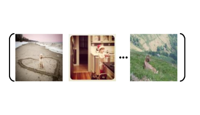
(a) Regular Mini-batch

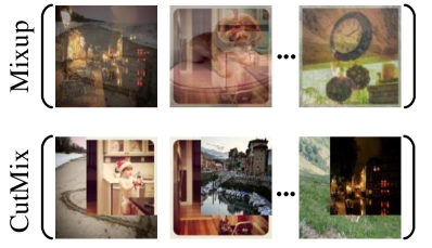
(b) Mix-style Mini-batch [3, 10]

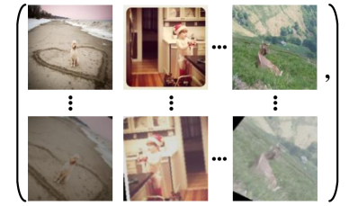
(c) BA Mini-batch [11]

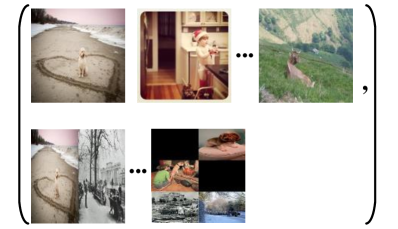
(d) SpliceMixed Mini-batch

Figure 1: Mini-batch comparisons between our SpliceMix and other methods. Our SpliceMix augments the image and label space similar to (b), and batch scale similar to (c), leading to good generalizability and fast convergence.

In MLIC, label dependency has been widely studied in [12, 13, 14, 15, 16], which builds the co-occurred relationship of different categories for boosting recognition performance. Nonetheless, as claimed in [17, 8], the label co-occurrence pattern learned from the training set could be contextually biased to identify a category when its typical context is absent. On the one hand, the semantic context (i.e., co-occurred relationship of categories) is crucial for improving MLIC. On the other hand, it may mislead the model in the scene of a category occurring in its unseen context. It is tricky to make a trade-off between learning label dependency and reducing co-occurred bias.

To some extent, Mix-style data augmentation methods naturally reduce the co-occurred bias. They usually generate a new image via mixing two images and their labels, which randomly produces a context-agnostic scene while losing the co-occurred relationship of categories. Two representative Mix-style methods, Mixup [3] and CutMix [10], have drawn lots of attention and their variants [18, 19, 20] have shown huge potential for many visual tasks recently. However, these methods are mainly designed for single-label images, neglecting the considerable gap between single- and multi-label images. As aforementioned, they fail to capture label dependency. Moreover, the small objects are easy to be messed in Mixup or lost in CutMix. Although some variants extract salient object regions of an image to paste to another image that may not suffer from the above pains, we want to claim that these extracted regions could be unreliable and they require additional knowledge [21] or complicated design [18, 22].

In this paper, we introduce a simple but effective, MLIC-adaptive Mix-style augmentation strategy, namely SpliceMix. The proposed method is not only targeted on MLIC, but also tackles another well-known issue of Mix-style methods that requires longer training epochs [3, 10]. Inspired by the fast convergence of Batch Augmentation (BA) [11], we keep both original regular mini-batch and generated samples to form a new SpliceMixed mini-batch. Fig. 1 compares the mini-batch used in regular training, Mix-style methods, BA, and SpliceMix. Comparing Figs. 1 (c) and (d), we show that SpliceMix increases the mini-batch size with only several mixed images, which is far less than batch scale of BA. Because each generated image is a splice of multiple images, a little increase of batch size is enough to guarantee fast convergence. Comparing mixed samples in Figs. 1 (b) and (d), we show that unlike existing Mix-style methods, our SpliceMix blends image semantics while preserving the entire objects, which produces an unusual scene for potential co-occurrences of both different objects and backgrounds-objects. In brief, our SpliceMix augments the sample space and batch scale simultaneously, where the former is to blend image semantics for alleviating co-occurred bias, and the latter allows us to learn label dependency from regular images and leads to fast convergence. A balance between learning label dependency and reducing co-occurred bias can be obtained in our SpliceMix. As shown in Fig. 1 (d) and Fig. 2, the mixed image in the form of a grid of multiple downsampled images contributes to cross-scale training with regular images, beneficial to small object recognition. Furthermore, the splice of regular images and mixed images enables the interactions between the two, which permits flexible extensions of SpliceMix. Hence, we offer a non-parametric design based on consistency learning, i.e., SpliceMix-CL, to show the extensibility of our SpliceMix.

Our contributions can be summarized as:

• To our best knowledge, our SpliceMix is the first data augmentation strategy designed for MLIC. The proposed SpliceMix is not only simple yet effective, but also orthogonal to existing MLIC methods, which can boost these methods remarkably.

• We offer a non-parametric, consistency learning-based extension to show the flexible extensibility of SpliceMix, where the fine knowledge of regular images is leveraged to learn better representation for mixed images.

• The two proposed methods achieve superior performance on several popular MLIC tasks and data sets. We also conduct on comprehensive analysis experiment to clarify the effectiveness of the proposed SpliceMix.

II Related Works

II-A Multi-label Image Classification.

Multi-label image classification (MLIC) is a challenging computer vision task and has attracted lots of attention. Existing MLIC methods prefer designing elaborate models to capture attention regions or label dependencies.

Discovering attention regions in a multi-label image is helpful to predict present categories or generate proposal candidates. Spatial Regularization Network (SRN) [23] learns weighted spatial attention maps with only image-level supervision and used multi-layer convolution to estimate class confidences from such attention maps. Different from SRN, [7] reuses classifier weights to obtain class-specific attention for discovering spatial discriminative regions. To generate informative proposal candidates, [24, 25, 26] utilize spatial attention to locate object regions. The difference among them is that [24, 26] extract local region features from feature maps directly instead of feeding local image regions into CNN again used in [25].

For label dependency-based methods, some techniques, e.g., Recurrent Neural Network (RNN) [27], Graph Neural Network (GNN) [28] and Transformer [29], usually are utilized to model label co-occurred correlation. CNN-RNN [30] learns joint image-label embedding and builds high-order label dependency via long short term memory recurrent neurons [31]. Beneficial from the excellent ability of modeling correlation GNN possesses, a series of methods [13, 16, 15] are proposed. [13, 32] consider label co-occurrence statistics as the adjacency matrix and then exploit GNN to map the label graph to class-dependent classifier or label embeddings. In view of poor model generalizability of label statistics-based graph, [12, 33] introduce dynamic graph to eliminate co-occurrence bias from the training set. In [14], Transformer Decoder is utilized to learn complex dependencies between feature maps and label embeddings. [34, 35] leverages both Encoder and Decoder in Transformer to learn intra-feature and feature-label correlations.

Two recent works [8, 36] indicate that exploiting label dependency may cause contextually biased recognition. Coincidentally, some previous MLIC researches [7, 12] suggest that the label co-occurrence information from limited training data is not enough for MLIC, which could lead to over-fitting. Therefore, we propose the SpliceMix to mitigate co-occurred bias via generating unusual scenes where the semantics of several images are blended and the learned label co-occurrence pattern is ameliorated.

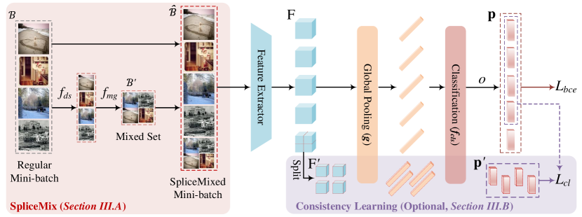
Figure 2: Overview of SpliceMix and SpliceMix-CL with a $2\times 2$ grid strategy. “$\stackrel{{\scriptstyle\bullet}}{{\longrightarrow}}$” denotes a function operation and “$\dashrightarrow$ ” denotes calculation without backpropagation. We simply introduce SpliceMix with the mini-batch samples whose size is 4. For generating unusual scene and preserving intact objects, SpliceMix makes a grid of downsampled images randomly sampled from the regular mini-batch to form the mixed set. The final SpliceMixed mini-batch is obtained by combining the regular mini-batch and mixed set. Furthermore, we offer a consistency learning-based design to show the flexible expansibility of our SpliceMix.

II-B Mix-style Augmentation.

Recently, Mix-style augmentation methods have shown promising performance in various single-label visual tasks, such as image classification [10, 19], super-resolution [37] and semantic segmentation [20]. As a founding one, Mixup [3] generates a new image by linearly combining two images and their labels. Since then, a bunch of Mix-style methods have been proposed, where CutMix [10] is a representative work that joints Mixup and Cutout [38] via replacing local regions with a patch from another image. Similar to the way of cut-and-paste in CutMix, some methods insert new patches to target images via leveraging smooth transition[39], attention maps [40], saliency information [22, 18]. Considering limited benefits of CutMix for visual Transformers, [19] mixes two images at token-level and generates the mixed label from content-based activations of a teacher network. [37] extends CutMix to the image super-resolution task where images with high resolution and low resolution consist of sample-pairs. [20] exploits predicted object boundaries to mix two unlabeled images for semi-supervised semantic segmentation.

Although Mix-style methods behave well in diverse single-label visual tasks, they are not suitable to MLIC because of more complicated image semantic and more categories in an multi-label image. For instance, cut-and-paste methods fail to assign the weight of labels from two images since a local patch cannot represent a multi-label images. In view of this, we aim to design a MLIC-adaptive augmentation strategy and exploit entire images to attend to mixing, which preserves all objects and results in reliable mixed labels.

II-C Batch Augmentation.

Different from previous augmentation methods, Batch Augmentation (BA) [11] increases the mini-batch size by replicating samples within the same mini-batch with different data augmentations, which accelerates model convergence and shows good generalization. The original BA is proposed to improve performance of training with large mini-batch size. [41] empirically shows that BA also works well for small mini-batch size. Whereas, BA still requires augmenting each image repeatedly for building a mini-batch, which is demanding. In our SpliceMix, we slightly increase the mini-batch size with mixed samples, each of which consists of multiple downsampled regular images. Even with only a few mixed samples, SpliceMix can significantly boost performance. Same to [41], we also allow fixed mini-batch size, i.e., keeping the same size to regular mini-batch via reducing regular samples to save space for mixed images.

III Methodology

This section will detail the proposed SpliceMix. Benefiting from our generated SpliceMixed mini-batch that enables interactions between original samples and their mixed samples, we also give a non-parametric extension based on consistency learning, namely SpliceMix-CL, for further improvement.

III-A SpliceMix

Given a mini-batch $\mathcal{B}=\{(\textbf{x}_{i},\textbf{y}_{i})|i\in[B]\}$, randomly sampling $B$ points from the training set, where x and y are an image and its label, respectively. As illustrated in Fig. 2, SpliceMix will generate a new mixed sample set $\mathcal{B}^{\prime}$ from $\mathcal{B}$, and then concatenate the original mini-batch and generated set to form the final mini-batch $\hat{\mathcal{B}}$ for training, i.e., $\hat{\mathcal{B}}=\mathcal{B}\cup\mathcal{B}^{\prime}$. Before turning sights to $\mathcal{B}^{\prime}$, we would like to clarify some terms used in the rest to avoid confusion. We call the original mini-batch $\mathcal{B}$ as the regular batch whose samples $(\textbf{x}$, $\textbf{y})$s are regular ones, the new mixed sample set $\mathcal{B}^{\prime}$ as the mixed set whose samples $(\textbf{x}^{\prime}$, $\textbf{y}^{\prime})$s are mixed ones and the generated final mini-batch $\hat{\mathcal{B}}$ as the SpliceMixed batch.

Mixture of images: The proposed SpliceMix aims to generate new images, preserving complete objects and producing an unusual scene for present categories. To achieve this, we make a grid of chosen regular images from $\mathcal{B}$ to form the mixed image. Keeping the resolution consistent with regular images, the chosen images are downsampled before griding, which brings a benefit of enabling the model to learn multi-scale information from regular images and their mixed ones. Let $f_{mg}$ denote the operation of making a grid and $f_{ds}$ denote the operation of downsampling. We can express the mixed image as

$$\textbf{x}^{\prime}=f_{mg}(\{f_{ds}(\textbf{x}_{i})|i\in\Omega\})~{},$$ (1)

where $\Omega$ is an index set of the regular batch that accounts for randomly selecting regular images to form the mixed image, e.g., the cardinality of $\Omega$ will be 4 if we want to obtain a mixed image with a $2\times 2$ grid of regular images.

In terms of the mixed images, they are a little similar to Mosaic used since YOLOv3 [42]. Here, we claim that the two methods are different in three points: 1) Mosaic needs bounding boxes of objects for annotation that cannot be applied to MLIC; 2) Objects in vanilla Mosaic are in original scale, not involved to cross-scale learning; 3) The mixed set is just a part of our SpliceMix where the regular images are kept, and both usual scenes (from regular images) and unusual scenes (from mixed images) can be learned.

Mixture of labels: Different from existing Mix-style methods that mix labels of two images via linear combination, the proposed SpliceMix sets the class label to be true if this class is present in the mixed image, formulated by

$$\textbf{y}^{\prime}=\cup_{i\in\Omega}\textbf{y}_{i}~{}.$$ (2)

The mixed label keeps multi-hot same to regular samples while containing more categories, which enriches the label diversity and is more suitable for MLIC training than the soft label used in existing Mix-style methods. Our SpliceMix method can be implemented readily in several lines of code. A PyTorch [43] implementation of $2\times 2$ mixed strategy is presented in Fig. 3.

Since we use the global images rather than local regions for mixing, there is almost no information depletion of present objects (except their resolutions are reduced) that means the label of each mixed image is reliable. More importantly, the proposed SpliceMix puts objects into a rare or complex scene, i.e., mixed scenes in our generated image. The model will build correlations among objects who may be co-occurred unusually and between objects and backgrounds where objects may be seldomly present. The mixed samples blend the image semantics and give the model more chances to see these potential scenes, alleviating the semantic and contextual bias and enhancing the model’s generalizability. On the other hand, we agree with the importance of inherent correlations from the training set and preserve the regular batch in our SpliceMixed batch in a BA-like way. The correlations on highly co-occurred objects still can be learned. In brief, our SpliceMixed batch consists of the regular batch and mixed set for the training time, from the former of which common label correlations are built and from the latter uncommon label correlations are reinforced. Both of them boost the final recognition and generalization performance.

import random, torch

from torch.nn.functional import interpolate as f_ds

from torchvision.utils import make_grid as f_mg

 

def SpliceMix(X, Y):

# X: (Batch size, Channels, Height, Width)

# Y: (Batch size, classes)

  B, C, H, W = X.shape

  Omega = random.sample(range(B), B//4*4)

  X_ds = f_ds(X[Omega], size=(H//2, W//2),

    mode=’bilinear’, align_corners=True)

  X_ = f_mg(X_ds, nrow=2, padding=0)

  X_ = X_.split(H, dim=1)

  X_ = torch.stack(X_, dim=0)

  Y_ = Y[Omega].view(B//4, 4, -1).sum(1)

  Y_[Y_>0] = 1

 

  X_hat = torch.cat((X, X_), dim=0)

  Y_hat = torch.cat((Y, Y_), dim=0)

  return X_hat, Y_hat

Figure 3: PyTorch implementation of SpliceMix with a $2\times 2$ grid strategy.

Setting of grids: As stated in Eq. (1), a mixed image is made from chosen regular images via two operations, i.e., $f_{mg}$ and $f_{ds}$, where the downsampling operation $f_{ds}$ is to resize the chosen regular images that lets the resolution of a mixed image match with that of regular images. For instance, given 4 regulars image whose resolutions are $448\times 448$ for generating a mixed image with a $2\times 2$ grid, we firstly resize them to $224\times 224$ and then make a $2\times 2$ grid of them to form the mixed image. The reduced scale $f_{ds}$ depends on which kind of the grid used for generating a mixed image. The grid number of different mixed images can be various. In other words, our SpliceMix allows to mix images with different combinations of grids to make up a mixed set, such as mixed images with grids of $1\times 2$, $2\times 2$, $2\times 3$, etc.

Here, we focus on the grid strategy introduced for SpliceMix. Several feasible grids are illustrated in Fig. 4. Accordingly, we can define a function family $\mathcal{F}_{mg}$ for sampling $f_{mg}$, that is

$$\mathcal{F}_{mg}=\{f^{r\times c}|r\in[G_{r}],c\in[G_{c}]\}~{},$$ (3)

where we rewrite $f_{mg}$ to $f^{r\times c}$, an operation of making a $r\times c$ grid, and $G_{r}$, $G_{c}$ denote the maximal rows and columns, respectively. Next, three types of the grid shown in Fig. 4 are discussed:

1. Symmetric grids: Sub-images in a symmetric grid are proportionally scaled from their regular images. Due to the same columns and rows in a symmetric grid, $f^{r\times c}$ is equal to $f^{c\times r}$. The number of grid dominates the complexity of the generated image. A more complicated mixed image needs more regular images whose resolution will be downsampled much more.

2. Asymmetric grids: The shape of sub-images in an asymmetric grid is squashed compared with their regular ones, which can be viewed as an additional transform besides rescaling. For a $f^{r\times c}$, if we keep the columns $c$ larger than the rows $r$ (e.g., the left figure in Fig. 4 (b)), the model may learn to recognize stretched objects well while losing its generalizability to flatten objects. To avoid this, we throw a coin with a flipped probability of 0.5 to decide which of $\{f^{r\times c},~{}f^{c\times r}\}$ will be adopted under this setting.

3. Grids with dropout: The goal of mixed images in the form of grids is to blend the image semantics and generate a new, unusual scene. Whereas, the generated scene may be over-complicated due to a large grid number, i.e. too many regular images attend to a mixed image. Therefore, we exploit a simple dropout mechanism to randomly mask a part of sub-images and corresponding labels in a mixed sample. After this, the complexity of a mixed image can be reduced, meanwhile the diversity of training samples is further enhanced.

$2\times 2$

(a) Sym. grids

$2\times 3$

$3\times 2$

(b) Asym. grids

$3\times 2-2$

(c) Grids w/ dp

Figure 4: Illustration of several feasible grid strategies for SpliceMix. Firstly, we assume that the regular images are square. Then, we can summary these grids as three types: (a) Symmetric grids with the same rows and columns; (b) Asymmetric grids with distinct rows and columns; (c) Grids with dropout where some sub-images are discarded randomly.

III-B SpliceMix-CL

The proposed SpliceMix allows interactions between sub-images from a mixed image and their regular versions, which means that the fine knowledge learned from regular images can be utilized to guide the model to learn better representation about coarse sub-images. In fact, there exist many techniques to help us learn consistent knowledge between regular images and sub-images, such as logits-based [44, 45] or feature-based [46, 47] knowledge distillation methods and class decoupling-based [32, 12] or attention-based [48] MLIC methods, where the knowledge distillation-aware methods are used for consistency learning and the MLIC-aware methods are used for task-specific knowledge extraction. Although these techniques may show promising performance with our SpliceMix, an elaborate model design is beyond our current study and we leave it to future work. Here, we offer a simple, non-parametric idea based on consistency learning [49], namely SpliceMix-CL, to show the extensibility of SpliceMix.

Assume that F is the last feature map extracted from a feature extractor, e.g., CNNs [1, 50], $g$ is a global pooling operation, $f_{cls}$ is a linear classifier, $o$ is sigmoid activation. Then, we can obtain the label prediction p of an input image, that is $\textbf{p}=o(f_{cls}(g(\text{F})))$. In a SpliceMixed batch, the classification loss, i.e., binary cross entropy (BCE) loss, is

$$\mathcal{L}_{bce}=\sum_{i}^{|\hat{\mathcal{B}}|}{-\textbf{y}_{i}log(\textbf{p}_{i})-(1-\textbf{y}_{i})log((1-\textbf{p}_{i}))}~{},$$ (4)

where $log$ denotes the element-wise logarithmic function. For convenience, we slightly abuse $(\textbf{x},\textbf{y})$ to denote any sample from $\hat{\mathcal{B}}$ and keep vector form of loss, each element of which is a class-specific loss. A scalar form of loss can be obtained by summing all class-specific loss values.

For each sub-image in a mixed image, we obtain its feature map $\text{F}^{\prime}$ via splitting F according to the grid form of the mixed image (see Fig. 2). By the way, we can simply exploit $f_{mg}$ to recover F from $\text{F}^{\prime}$s: $\text{F}=f_{mg}(\{\text{F}^{\prime}_{i}|i\in\Omega\})$, where the subscript $i$ indicates the $i$-th image in $\mathcal{B}$ attending to the mixed image and we reuse such subscript to indicate the feature map of a sub-image since a regular image attends to mixed images at most once. Consequently, the prediction $\textbf{p}^{\prime}$ of a sub-image can be calculated by $o(f_{cls}(g(\text{F}^{\prime})))$. For consistency learning between sub-images and their regular images, we utilize the prediction distribution p from a regular image to supervise the output of its corresponding sub-image, whose objective can be formulated by

$$\mathcal{L}_{cl}=\sum_{i}^{|\mathcal{B}^{\prime}|}\sum_{j\in\Omega_{i}}{-\bar{\textbf{p}}_{j}log(\textbf{p}^{\prime}_{j})-(1-\bar{\textbf{p}}_{j})log(1-\textbf{p}^{\prime}_{j})}~{},$$ (5)

where $\bar{\textbf{p}}$ is a copy of p without backpropagation and we reuse the subscript $j$ to $\textbf{p}^{\prime}$ that is obtained from the sub-image of the $i$-th mixed image corresponding to $j$-th regular image (the subscript $i$ is omitted for convenience).

Finally, the total training objective of SpliceMix-CL is

$$\mathcal{L}=\mathcal{L}_{bce}+\mathcal{L}_{cl}~{}.$$ (6)

Although it seems that the consistency learning loss is only imposed on the pair of regular images and their sub-images, we claim that it is not simply equal to learning cross-scale knowledge. The better representation of sub-images helps the model discover possibly overlooked objects present in a mixed image, which is beneficial for blending image semantics and improving our SpliceMix.

IV Experiments

In this section, we first introduce experimental settings including evaluation metrics and our training details. Next, convergence analyses are given and the proposed methods are verified via plentiful experiments. Finally, we conduct performance analyses to discuss the proposed methods detailedly.

IV-A Experimental settings

Evaluation metrics: We follow previous works [13, 12], adopting mean of Average Precision (mAP) as the primary metric. Overall precision (OP), recall (OR), F1-score (OF1) and per-class precision (CP), recall (CR), F1-score (CF1) and their top-3 versions are also utilized to evaluate our results. All metric are in %. For all metrics except mAP, we set a category to be positive if its prediction is larger than 0.5, vice versa.

Training details: For the proposed methods and compared methods, we use ResNet-101 [1] as the base model where the last global average pooling is replaced with global max pooling that is a common setting [13, 12] to achieve good results for MLIC. We choose SGD as our optimizer with momentum of 0.9 and weight decay of $10^{-4}$. The output dimension of the last fully connected (fc) layer in ResNet-101 is changed according to the class number of various data sets. We set the learning rate of all layers except the last fc layer to be one-tenth of the given learning rate. During training, we adopt the data augmentation suggested in [13, 33], i.e., the input image is randomly cropped and resized to 448 × 448 with horizontal flips. We train our model for 80 epochs and decay the learning rate by a factor of 0.1 at 40-th and 60-th epoch. For our SpliceMix, we do not seek the optimal grid strategy deliberately and randomly sample $f_{mg}$ from $\mathcal{F}_{mg}=\{f^{1\times 2},f^{2\times 2},f^{2\times 3}\}$ with a probability of 0.3 to use a random dropout from 1 to $r\times c-1$ per batch. The cardinality of the mixed set is set to a quarter of the regular batch size, i.e., $|\mathcal{B}^{\prime}|=\frac{1}{4}|\mathcal{B}|$. All experiments are implemented based on PyTorch [43].

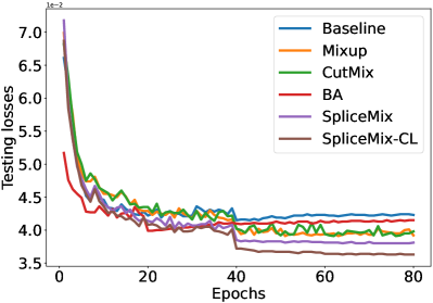
(a) Convergence

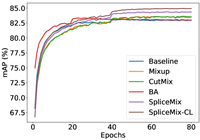
(b) Classification performance

Figure 5: Comparisons of convergence and classification performance on MS-COCO [51]. We report the results of the total 80 epochs. ResNet-101 is the baseline for all methods. Except for BA, whose learning rate is decayed at 20-th and 40-th epoch, all other methods decay the learning rate at 40-th and 60-th epoch.

TABLE I: Comparisons with state-of-the-art methods on MS-COCO. The best and second best results (except the methods marked by “^∗”) are highlighted in purple and cyan, respectively. The same highlighted way is used for the remaining tables.

Method	mAP	All						Top 3
		CP	CR	CF1	OP	OR	OF1	CP	CR	CF1	OP	OR	OF1
DSDL [52]	81.7	84.1	70.4	76.7	85.1	73.9	79.1	88.1	62.9	73.4	89.6	65.3	75.6
CSRA [7]	83.5	84.1	72.5	77.9	85.6	75.7	80.3	88.5	64.2	74.4	90.4	66.4	76.5
SST [53]	84.2	86.1	72.1	78.5	87.2	75.4	80.8	89.8	64.1	74.8	91.5	66.4	76.9
CCD [8]	84.0	87.2	70.9	77.3	88.8	74.6	81.1	89.7	63.9	72.9	92.0	66.5	77.2
IDA-R101 [36]	84.3	-	-	78.5	-	-	81.1	-	-	73.6	-	-	77.3
Baseline	83.0	85.0	72.0	77.9	86.9	75.2	80.3	89.0	64.1	74.5	90.7	66.3	76.6
Mixup [3]	83.7	84.9	72.8	78.4	86.5	75.7	80.7	89.3	64.8	75.1	91.1	66.5	76.9
CutMix [10]	83.5	84.6	72.9	78.3	86.2	75.5	80.5	89.0	64.8	75.0	90.9	66.3	76.7
ResizeMix [54]	83.1	86.1	71.0	77.8	88.0	73.4	80.1	90.1	64.0	74.8	91.7	65.3	76.3
RecursiveMix [55]	83.4	86.9	70.4	77.8	88.8	72.6	79.9	90.3	63.8	74.7	92.3	64.8	76.1
BA [11]	83.3	84.8	72.5	78.2	85.8	75.6	80.4	89.0	64.4	74.7	90.4	66.5	76.7
SpliceMix	84.4	84.8	74.2	79.1	86.2	77.0	81.3	89.2	65.6	75.6	91.0	67.2	77.3
SpliceMix-CL	84.9	87.4	73.2	79.7	88.2	76.3	81.8	90.7	65.1	75.8	92.1	67.1	77.6
SpliceMix∗	85.8	85.1	76.6	80.6	86.4	78.7	82.3	89.6	67.3	76.9	91.4	68.2	78.1
SpliceMix-CL∗	86.4	85.5	76.9	81.0	87.0	79.0	82.8	89.8	67.6	77.1	91.7	68.6	78.5

IV-B Convergence Analyses

As we claimed before, our SpliceMix can lead to faster convergence with lower testing loss. Compared with two popular Mix-style methods (Mixup [3] and CutMix [10]), BA [11] and the baseline ResNet-101, we present the results of convergence and classification performance of testing time in Fig. 5. It can be readily seen that our SpliceMix and SpliceMix-CL take the top-2 lowest testing loss and highest mAP. Further, from Fig. 5 (a), we can discover that 1) the baseline and BA fall into over-fitting after 40/20 epochs, which results in a little drop of mAP as shown in Fig. 5 (b) since its testing loss turns to increase slightly; 2) both Mixup and CutMix fail to converge steadily, which leads to fluctuant classification performance in Fig. 5 (b). As suggested in [10], Mixup and CutMix require longer training epochs (twice of the regular training) to achieve good performance. We try our best to follow such epoch setting of [10] originally leveraged for single-label image classification, while obtaining worse results for MLIC. Hence, we keep the same training setting to our proposed methods for the two Mix-style methods, which is also the optimal setting in our tries. In our proposed SpliceMix and SpliceMix-CL, drawbacks of BA and two Mix-style methods are overcome. In other words, SpliceMix reduces the risk of over-fitting in the BA and has a steadier and lower convergence bound compared to both Mix-style methods and BA. Furthermore, the proposed SpliceMix-CL has the lowest testing loss and highest mAP shown in Fig. 5, which reveals the excellent extensibility of SpliceMix.

IV-C Multi-label Image Classification (MLIC)

We evaluate the proposed SpliceMix and SpliceMix-CL on two MLIC tasks, i.e., regular MLIC and MLIC with missing labels, where common data sets MS-COCO 2014 [51] and Pascal VOC 2007 [56] are adopted.

IV-C1 Regular MLIC

MS-COCO 2014: Microsoft COCO 2014, short for MS-COCO, is a widely used benchmark for MLIC. There are 82,081 images in the training set and 40,137 images in the validation set with total 80 common objects categories. Since labels of the test set are unavailable, we compare our methods to other methods on the validation set. The learning rate for MS-COCO is set to 0.05 and the batch size is 32. The comparison results are presented in Table I. It’s worth noting that SpliceMix can achieve comparable performance in ImageNet [57] classification. Hence, we also report the results of the two proposed methods adopting ImageNet pre-training based on SpliceMix and mark them by “^∗”, same for Tables II and III.

To ensure the fairness for compared methods, we make a grid search of the $\alpha$ in Mixup [3] and CutMix [10] from 0.1 to 1 with a step of 0.2. We find that $\alpha=0.5$ is optimal for the two methods on both MS-COCO and Pascal VOC 2007. For BA, we choose the times of replicating samples (i.e., $M$ in [11]) from $\{2,4,6\}$ and find that replicating samples twice achieves the highest performance. As shown in Table I, our two methods have the best performance in most metrics. In compared MLIC methods, CCD [8] and IDA-R101 [36] are designed for removing co-occurred bias which obtain high mAP. With the similar objective, we blend multiple images to generate an unusual scene for existing categories. Although our SpliceMix is just a simple augmentation method, it achieves superior performance to two contextually debiased models. Moreover, our SpliceMix-CL also shows an excellent improvement, compared to SpliceMix and current advance methods, which suggests the large potential of expanding our SpliceMix. From the last two rows of Table I, we can see that SpliceMix-based ImageNet pre-training performs well in the MLIC task.

Pascal VOC 2007: Pascal Visual Object Classes Challenge (VOC 2007) is the most used data set in MLIC. It consists of 20 object categories from 9,963 images. We use the trainval set (5,011 images) for training and the test set (4,952 images) for evaluation. The learning rate for Pascal VOC 2007 is set to 0.01 and the batch size is 16. Considering that some current MLIC methods tend to train Pascal VOC 2007 not only with ImageNet pre-training but also with MS-COCO pre-training, where the latter can achieve better performance empirically, we give results on pre-training from ImageNet and MS-COCO, respectively.

The comparison of our methods and other methods is listed in Table II. We can see that our SpliceMix and SpliceMix-CL outperform all other methods. In compared Mix-style methods, ResizeMix [54] and RecursiveMix [55] are highly customized for single-label images that show poor performance (also see Table I), that is unsuitable for MLIC. Notably, comparing the mAP of four previous Mix-style methods on MS-COCO pre-training that is inferior to the baseline, our SpliceMix enjoys the gain from MS-COCO hugely.

TABLE II: Comparisons with state-of-the-art methods on Pascal VOC 2007.

Method	mAP
	ImageNet pre.	MS-COCO pre.
SSGRL [32]	93.4	95.0
ML-GCN [13]	94.0	-
ADDGCN [12]	-	96.0
CCD [8]	-	95.8
ASL [48]	94.6	95.8
Baseline [1]	93.3	95.8
Mixup [3]	93.8	95.6
CutMix [10]	93.8	95.5
ResizeMix [54]	93.3	95.5
RecursiveMix [55]	93.3	95.7
BA [11]	93.9	95.6
SpliceMix	94.6	96.1
SpliceMix-CL	94.8	96.3
SpliceMix∗	95.3	96.5
SpliceMix-CL∗	95.5	96.7

IV-C2 MLIC with Missing Labels

In real scenarios, it is usually difficult to collect all true labels of a multi-label image. An image may be annotated with only partial positive labels, which hinders the performance of MLIC. Multi-label learning with missing/partial-annotated labels has been a hot spot in recent researches [58, 59]. In a popular setting [58], partial positive and negative labels are accurately known and for unknown labels, they can be either positive or negative. In this paper, we follow the previous work [59] and further relax such setting, where no accurate negative labels are required. In other words, only limited positive labels are known in our missing label setting which is more flexible in practice.

We conduct experiments on MS-COCO with missing label setting. Following the setting of [59], we randomly drop positive labels with different ratios ($80\%$ and $100\%$ but keeping single positive label per image) for constructing the training set. Finally, the remaining labels are $40\%$ of original positive labels and single positive label per image. Keeping the same architecture to previous work [59], we adopt ResNet-50 with global max pooling as our baseline. Table III lists the comparison results, where methods in the first block is originally reported in [59], and we implement the remaining methods for comparisons. It is easy to discover that our methods consistently outperform all other methods. Compared to the baseline, the proposed SpliceMix shows more robust results as the decrease of left label ratio, which indicates good capacities of our SpliceMix to handle the problem of missing labels. In addition, the ImageNet pre-training via SpliceMix helps our two methods boost a lot, which exhibits its advantage in model pre-training.

TABLE III: Comparisons on MS-COCO with different missing ratio.

Method	$40\%$ label left			single label
	mAP	CF1	OF1	mAP	CF1	OF1
BCE-LS[60]	73.1	44.9	41.2	70.5	40.9	37.3
WAN[60]	72.1	62.8	64.9	70.2	58.0	58.6
Focal[61]	71.7	48.7	44.0	70.2	47.0	41.4
ASL[48]	72.7	67.7	71.7	71.8	44.8	37.9
SPLC[59]	75.7	67.9	73.3	73.2	61.6	67.4
Baseline[1]	74.4	69.3	73.5	72.2	61.7	67.9
Mixup[3]	75.6	70.3	74.4	73.6	66.9	71.6
CutMix[10]	75.5	70.3	74.5	73.6	67.3	71.6
ResizeMix [54]	75.3	69.5	73.8	73.4	67.0	71.7
RecursiveMix [55]	74.9	69.3	73.8	73.0	66.4	70.9
BA [11]	74.6	69.7	73.8	72.5	65.7	70.0
SpliceMix	76.0	71.0	75.1	74.4	67.5	72.0
SpliceMix-CL	76.9	71.4	75.5	74.7	67.5	72.2
SpliceMix∗	78.6	73.5	76.5	77.0	67.5	70.8
SpliceMix-CL∗	79.6	69.7	73.8	77.6	70.7	74.2

TABLE IV: The performance improvement to state-of-the-art MLIC methods using SpliceMix. $\uparrow$ denotes the performance gain and $\downarrow$ denotes the performance drop.

Method	mAP	All						Top 3
		CP	CR	CF1	OP	OR	OF1	CP	CR	CF1	OP	OR	OF1
MLGCN [13]	83.0	85.1	72.0	78.0	85.8	75.4	80.3	89.2	64.1	74.6	90.5	66.5	76.7
+SpliceMix	84.2 (1.2$\uparrow$)	87.1 (2.0$\uparrow$)	72.3 (0.3$\uparrow$)	79.1 (1.1$\uparrow$)	87.8 (2.0$\uparrow$)	75.3 (0.1$\downarrow$)	81.1 (0.8$\uparrow$)	90.4 (1.2$\uparrow$)	64.8 (0.7$\uparrow$)	75.5 (0.9$\uparrow$)	91.7 (1.2$\uparrow$)	66.6 (0.1$\uparrow$)	77.1 (0.4$\uparrow$)
SSGRL [32]	83.8	89.9	68.5	76.8	91.3	70.8	79.7	91.9	62.5	72.7	93.8	64.1	76.2
+SpliceMix	84.7 (0.9$\uparrow$)	87.3 (2.6$\downarrow$)	72.7 (4.2$\uparrow$)	79.3 (2.5$\uparrow$)	87.9 (3.4$\downarrow$)	75.8 (5.0$\uparrow$)	81.4 (1.7$\uparrow$)	90.5 (1.4$\downarrow$)	64.6 (2.1$\uparrow$)	75.4 (2.7$\uparrow$)	91.9 (1.9$\downarrow$)	66.8 (2.7$\uparrow$)	77.4 (1.2$\uparrow$)
ADDGCN (576) [12]	85.2	84.7	75.9	80.1	84.9	79.4	82.0	88.8	66.2	75.8	90.3	68.5	77.9
+SpliceMix	85.8 (0.6$\uparrow$)	87.6 (2.9$\uparrow$)	74.2 (1.7$\downarrow$)	80.3 (0.2$\uparrow$)	88.6 (3.7$\uparrow$)	77.1 (2.3$\downarrow$)	82.5 (0.5$\uparrow$)	91.0 (2.2$\uparrow$)	65.5 (0.7$\downarrow$)	76.2 (0.4$\uparrow$)	92.5 (2.2$\uparrow$)	67.5 (1.0$\downarrow$)	78.1 (0.2$\uparrow$)
TDRG [33]	84.6	86.0	73.1	79.0	86.6	76.4	81.2	89.9	64.4	75.0	91.2	67.0	77.2
+SpliceMix	85.1 (0.5$\uparrow$)	86.7 (0.7$\uparrow$)	74.0 (0.9$\uparrow$)	79.8 (0.8$\uparrow$)	87.4 (0.8$\uparrow$)	77.0 (0.6$\uparrow$)	81.9 (0.7$\uparrow$)	90.3 (0.4$\uparrow$)	65.4 (1.0$\uparrow$)	75.8 (0.8$\uparrow$)	91.7 (0.5$\uparrow$)	67.5 (0.5$\uparrow$)	77.7 (0.5$\uparrow$)
ShuffleNetV2 [62]	69.7	80.2	51.3	62.5	85.5	58.9	69.7	82.8	47.0	60.0	88.6	54.3	67.3
+SpliceMix	70.7 (1.0$\uparrow$)	77.9 (2.3$\downarrow$)	56.2 (4.9$\uparrow$)	65.5 (3.0$\uparrow$)	83.6 (1.9$\downarrow$)	62.6 (3.7$\uparrow$)	71.6 (1.9$\uparrow$)	81.1 (1.7$\downarrow$)	50.7 (3.7$\uparrow$)	62.4 (2.4$\uparrow$)	88.1 (0.5$\downarrow$)	56.6 (2.3$\uparrow$)	68.9 (1.6$\uparrow$)
ResNet-101  [1]	80.5	83.4	68.0	74.9	86.3	72.5	78.9	87.0	60.5	71.4	90.6	64.3	75.2
+SpliceMix	81.9 (1.4$\uparrow$)	79.2 (4.2$\downarrow$)	74.1 (6.1$\uparrow$)	76.6 (1.7$\uparrow$)	83.2 (3.1$\downarrow$)	77.1 (4.6$\uparrow$)	80.0 (1.1$\uparrow$)	84.5 (2.5$\downarrow$)	65.1 (4.6$\uparrow$)	73.5 (2.1$\uparrow$)	89.2 (1.4$\downarrow$)	66.8 (2.5$\uparrow$)	76.4 (1.2$\uparrow$)
ViT-B (384) [63]	86.6	87.5	74.9	80.7	88.7	77.6	82.8	90.9	66.6	76.9	92.7	68.4	78.7
+SpliceMix	87.5 (0.9$\uparrow$)	86.6 (0.9$\downarrow$)	78.0 (3.1$\uparrow$)	82.1 (1.4$\uparrow$)	87.7 (1.0$\downarrow$)	80.2 (2.6$\uparrow$)	83.8 (1.0$\uparrow$)	91.4 (0.5$\uparrow$)	68.4 (1.8$\uparrow$)	78.3 (1.4$\uparrow$)	92.4 (0.3$\downarrow$)	69.5 (1.1$\uparrow$)	79.4 (0.7$\uparrow$)
Swin-B (224) [64]	84.9	86.4	73.7	79.6	87.5	76.3	81.5	89.9	65.8	76.0	91.6	67.7	77.8
+SpliceMix	85.8 (0.9$\uparrow$)	85.4 (1.0$\downarrow$)	76.2 (2.5$\uparrow$)	80.5 (0.9$\uparrow$)	86.6 (0.9$\downarrow$)	78.6 (2.3$\uparrow$)	82.4 (0.9$\uparrow$)	90.2 (0.3$\uparrow$)	67.5 (1.7$\uparrow$)	77.2 (1.2$\uparrow$)	91.4 (0.2$\downarrow$)	68.9 (1.2$\uparrow$)	78.6 (0.8$\uparrow$)

IV-D Improvement to State-of-the-Art Methods

The proposed SpliceMix is a simple and effective augmentation strategy, which is orthogonal to existing MLIC methods and various backbone models. We evaluate our SpliceMix on the performance improvement to four state-of-the-art MLIC methods and four advanced backbones. The result is listed in Table IV. In compared methods, Visual Transformer (ViT) [63] is fine-tuned from SWAG [65] weight and Swin Transformer (short for Swin) [64] is pre-trained by ImageNet-22k [66]. All other methods use the ImageNet-1k pre-training.

It can be seen from Table IV, SpliceMix consistently improves all methods in primary metrics that are mAP, CF1 and OF1. For state-of-the-art MLIC methods, SpliceMix boosts them at least 0.5% and at most 1.2% mAP. For advanced backbones including a lightweight network (ShuffleNetV2 [62]), a classical CNN (ResNet-101 [1]) and two Transformer-based models (ViT-B and Swin-B), SpliceMix boosts them at least 0.9% and at most 1.4% mAP.

Multi-label image data sets usually have the issue of positive-negative imbalance [48]. A model could predict positive classes with low confidences, leading to high precision and low recall. Our SpliceMix constructs the label of a mixed image by a union of regular labels, which improves the ratio of positive-negative classes in some degree. Comparing the CP and CR, or OP and OR of four backbones in Table IV, we can discover that CP and OP have larger values than CR and OR due to too low confidences of positive classes. In our SpliceMix, such circumstance is mitigated. SpliceMix helps these backbones increase the CR and OR with an acceptable drop of CP and OP. As a result, SpliceMix improves the CF1 and OF1 significantly.

IV-E Small Object Recognition

A multi-label image usually contains multiple objects whose scales are fickle. Small objects could be ignored due to low resolution [33] or global pooling operation [34], resulting in poor recognition performance. In SpliceMix, we deal with small object recognition problem via exploiting information learned from images with different scales in the same batch efficiently. Besides, we also introduce a consistency learning-based design to bridge the gap of objects between regular images and mixed images to further improve SpliceMix.

We conduct experiments on MS-COCO to evaluate our methods in boosting small object recognition performance. In fact, different from the object detection task, it is impossible to recognize all objects in a multi-label image due to the lack of bounding boxes, although small objects always impair the performance of MLIC. We calculate the average object size of each categories by the bounding box offered in the MS-COCO data set. And then, we sort all categories from small to large according to the average object size. The AP improvement of our methods compared to the baseline (ResNet-101) is illustrated in Fig. 6. The proposed SpliceMix and SpliceMix-CL boost the small object recognition performance remarkably. The mean AP improvement of the top-20 smallest and largest categories in SpliceMix is 1.8% and 0.9%, respectively. SpliceMix boosts the AP of small objects more than twice that of large objects. Comparing Figs. 6 (a) and (b), SpliceMix-CL further improves SpliceMix in almost all selected categories, which indicates the effectiveness of our consistency learning-based design and the flexible extensibility of SpliceMix.

Note that the improvement of small object recognition is not only due to cross-scale training in our SpliceMix, but also owing to semantic blending learning. Small objects tend to have poor correlation to other objects because they could be neglected easily. Our SpliceMix enhances the label dependency and reduces the co-occurred bias that can contribute to identify small objects both in their usual and unusual scenes.

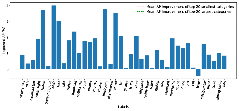
(a) SpliceMix

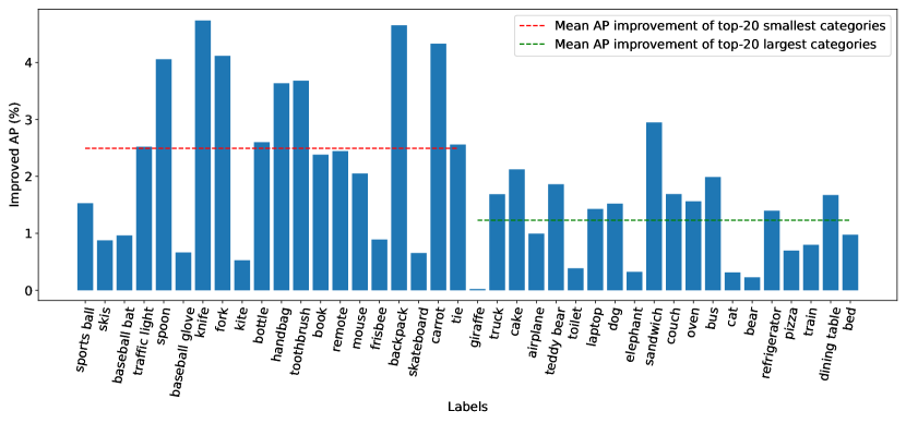
(b) SpliceMix-CL

Figure 6: AP improvement of our methods boosting the baseline. For clear presentation, the top-20 smallest and largest categories are selected from left to right.

IV-F Inference with Low Resolution Images

In practical applications, the quality of query images may be not guaranteed. A model could be trained with high resolution images, while inferring images under a low resolution circumstance. The model performance will be hindered severely, due to the large resolution discrepancy between training and inferring [67]. Our SpliceMix trains regular images and their downsampled versions simultaneously, which is beneficial to mitigate the above issue.

Fig. 7 compares the inference performance with various image resolutions on MS-COCO. We can see that low resolutions degrade the performance of all methods. The mAP of four compared methods drops rapidly as the inferring resolution declines. However, our SpliceMix and SpliceMix-CL present good robustness to low resolution images. For instance, the mAP of SpliceMix surpasses compared methods over at least 10% in the ultra-low $64\times 64$ resolution. Besides, we may discover that SpliceMix-CL outperforms SpliceMix in the resolutions of $448\times 448$ and $224\times 224$, while losing its superiority in $112\times 112$ and $64\times 64$. In the default setting of SpliceMix (see Sec. IV-A), at least one of the height and width of a downsampled image is 224. The consistency learning between regular images and their downsampled images may focus on bridging the gap between $448\times 448$ and $224\times 224$, resulting in sub-optimal performance to lower resolutions.

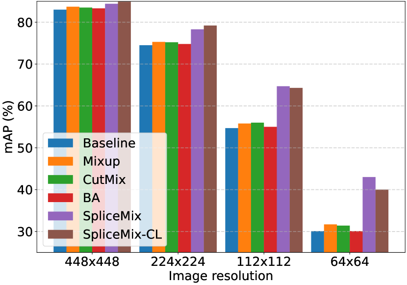
Figure 7: Comparisons on various image resolutions in inferring phase. All methods are trained with $448\times 448$ image resolution and inferred with the resolutions of $448\times 448$, $224\times 224$, $112\times 112$, and $64\times 64$, respectively.

IV-G Performance Analyses

IV-G1 Label Dependency and Co-occurred Bias

In the multi-label image classification task, it is challenging to balance the label dependency and co-occurred bias. Capturing label dependency is beneficial for a model to recognize co-occurred categories in their usual context. However, it may hamper the model generalizability of recognizing categories occurring in their unusual context. The proposed SpliceMix learns label dependency from the regular batch and reduces co-occurred bias via semantic blending learning in the mixed set. The ameliorated label dependency can be built from the trade-off between learning label dependency and reducing co-occurred bias.

To verify this, we first give the result of label dependency learning in our SpliceMix. The T-SNE visualization on the classifier weight pre-trained on MS-COCO [51] is presented in Fig. 8. Compared to the baseline (ResNet-101 [1]), SpliceMix can capture better label correlation. For example, the categories “cup” and “bowl” lose their co-occurrence relationships in the baseline shown in Fig. 8 (a). However, in our SpliceMix, the two categories are near their correlated categories, which accurately reflects category relationships in their super set “kitchen”. Moreover, SpliceMix also builds improved label dependencies for other super sets, such as “electronic”, “animal” and “outdoor”.

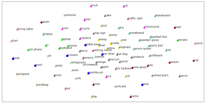
(a) Baseline

(b) SpliceMix

Figure 8: T-SNE Visualization on the classifier weight of the baseline and SpliceMix. Categories in the same shape and color belong to the same super set offered by MS-COCO.

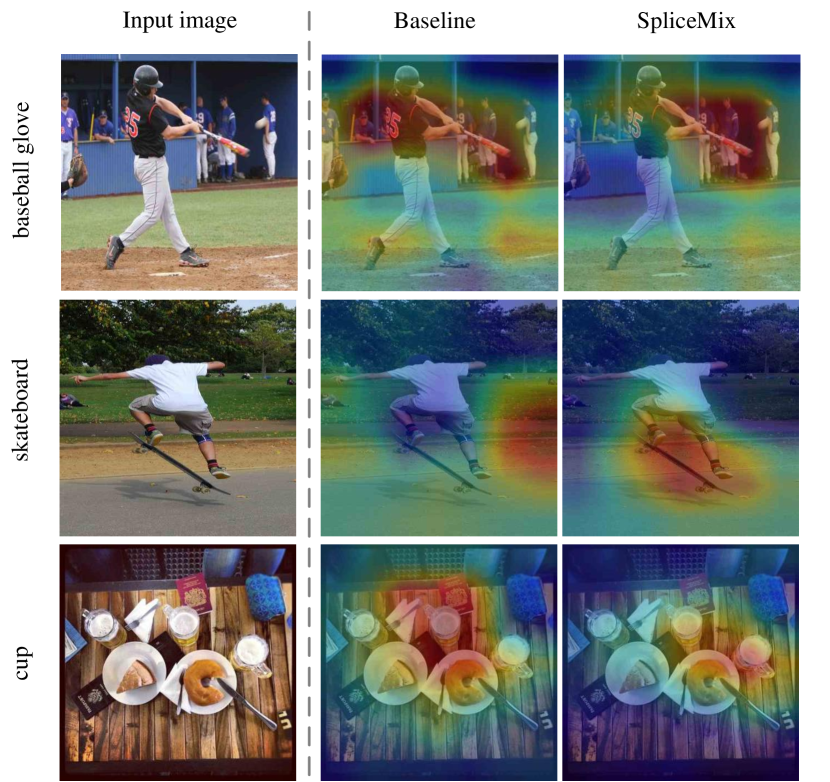
Figure 9: CAM visualization of highly biased categories. The biased category pairs (baseball glove, person), (skateboard, person) and (cup, dining table) are in the 20 most biased category pairs.

For studying co-occurred bias, we follow the previous work [17] and conduct experiments on COCO-Stuff [68] that is an augmented version of MS-COCO 2017 with pixel-wise annotations for 91 stuff classes. We run our SpliceMix based on a re-implementation of [17]. Before evaluation, the 20 most biased category pairs are determined. For each biased category pair $(b,c)$, the test set can be divided into three sets: co-occurred images that contain both $b$ and $c$, exclusive images that contain $b$ but not $c$, and other images that do not contain $b$. Then, two test distributions can be constructed: 1) the “exclusive” distribution containing exclusive and other images and 2) the “co-occur” distribution containing co-occurred and other images. More details can be found in [17, 69]. The classification result is reported in Table V.

TABLE V: Performance comparison on exclusive distribution and co-occurred distribution. The mAP metric is reported.

Method	Exclusive	Co-occur	Exclusive+Co-occur
Baseline	21.6	65.5	87.1
SpliceMix	23.7	66.4	90.1

As we can see, SpliceMix improves the baseline (ResNet-50) by 2.1% mAP in exclusive distribution, which means our SpliceMix has better performance of recognizing categories when these categories occur in their unusual context. The co-occurred bias is mitigated by SpliceMix. In addition, for co-occurred categories, SpliceMix also outperforms the baseline by 0.9% mAP, which indicates ameliorated label dependency is learned in SpliceMix. A good trade-off between learning label dependency and reducing co-occurred bias can be sought. Furthermore, we compare the class activation map (CAM) [70] of the baseline and SpliceMix to present the issue existing in highly biased category pairs. As shown in Fig. 9, for the categories “baseball glove” and “cup”, the baseline locates more areas on the objective co-occurred categories, i.e., “person” and “dining table”, respectively. Only a little information of the query category can be learned which may be less discriminative for recognizing this category in its rare context. Oppositely, our SpliceMix locates “baseball glove” and “cup” intensively, which means that less co-occurred bias is induced. Let us see the second row of Fig. 9, the baseline fails to discover the object, which could be because the baseline can not identify the easy category “person”, resulting in that its correlated object (i.e., “skateboard”) is ignored. In our SpliceMix, such strong co-occurred relationship is not required. Hence, SpliceMix can recognize and locate “skateboard” effectively.

IV-G2 Ablation Studies

We study the effectiveness of the proposed methods from four aspects, i.e., cross-scale learning, semantic blending learning, batch splice and consistency learning, where the batch splice denotes the splice of the regular batch and mixed set (see Fig. 2). Considering that the batch splice and consistency learning is not orthogonal to cross-scale learning and semantic blending learning, we will discuss them among the latter. The experiments are conducted on MS-COCO with a $2\times 2$ grid strategy of SpliceMix and the results are listed in Table VI where the denotations $f_{ds}$ and $f_{mg}$ account for cross-scale learning and semantic blending learning, respectively (see Eq. (1)). $\cup$ denotes batch splice and $L_{cl}$ denotes consistency learning (see Eq. (5))..

Cross-scale learning: For removing the component of semantic blending, we adopt the setting of grids with dropout, i.e., $2\times 2-3$. Then, the mixed image is degraded to a downsampled image merely, which is corresponding to ($f_{ds}+\cup$) in Table VI. The consistency learning can be built from regular images and their downsampled images, corresponding to ($f_{ds}+\cup+L_{cl}$). To reach only $f_{ds}$, we downsample regular images to half of their height and width, and then train downsampled images after training regular batch. From Table VI, we can see that the batch splice improves the performance of cross-scale learning, which indicates the cross-scale information from the same batch is better than that from different batch. Further, with the consistency learning, the performance of cross-scale learning is boosted a lot. In our SpliceMix-CL, the knowledge of fine regular images is leveraged to guide the model to learn better representation of coarse mixed images. In this part of only cross-scale learning, the gain from consistency learning is obvious, and it will be more with the joint of semantic blending learning. Besides, owing to cross-scale learning, SpliceMix has an advantage of recognizing small objects, even when the query image is low-resolution (see Sec. IV-F).

Semantic blending learning: Semantic blending in our SpliceMix is implemented by making a grid of several downsampled regular images. The object information is lossless except the resolution, which better contributes to producing an unusual scene for present objects than current Mix-style methods [3, 10]. Evaluating the semantic blending learning separately is spiny. Therefore, we evaluate its performance by incremental comparisons. Comparing ($f_{ds}+\cup$) to ($f_{ds}+f_{mg}+\cup$) in Table VI, we can find that with semantic blending, the mAP is improved by 0.7% that suggests the effectiveness of semantic blending learning to mitigate the co-occurred bias. We may also notice that ($f_{ds}+f_{mg}$) without batch splice harms the performance a little compared to the baseline, from which we can realize the importance of batch splice.

TABLE VI: Ablation study for different components of SpliceMix and SpliceMix-CL. The first row is the results of the baseline and the last two rows are the results of SpliceMix and SpliceMix-CL, respectively.

$f_{ds}$	$f_{mg}$	$\cup$	$L_{cl}$	mAP	CF1	OF1
				83.0	77.9	80.3
✓				83.2	77.3	80.0
✓		✓		83.5	78.4	80.6
✓		✓	✓	84.1	78.5	80.7
✓	✓			82.9	77.8	80.2
✓	✓	✓		84.2	78.7	80.9
✓	✓	✓	✓	84.7	79.7	81.7

IV-G3 Ways of Batch Splice

The batch splice in our SpliceMix is a combination of the mixed set and regular batch, where the final SpliceMixed batch size is increased a little due to the introduction of the mixed set. Another way to batch splice is combining the mixed set and regular images that do not attend to mixing. In other words, there is no repeated image in such final batch whose size is less than the regular batch. We conduct experiments on MS-COCO to compare the performance of the batch splice used in our SpliceMix and the batch splice without repeated images. In our SpliceMix, the regular batch size is 32 and the cardinality of the mixed set is 8. To reach the same final batch size to SpliceMix, for the compared method, we choose the number of regular images and mixed images from the pairs of $\{(32,8),(20,20),(0,40)\}$, where the pair of $(0,40)$ only uses the mixed images for training. A $2\times 2$ grid strategy is adopted for all methods.

Table VII reports the results of the two ways of batch splice. When only mixed images are used (i.e., $(0,40)$ in Table VII) for training, the model performance degrades a lot. In the compared method, the mAP increases gradually with the decreased number of mixed images, which indicates the splice with regular images contributes to boosting performance. However, the performance boost of the compared methods is limited. With the same number of regular images and mixed images to our SpliceMix, the compared method achieves 83.7% mAP that is less than SpliceMix. As shown in Table VII, the batch splice used in our SpliceMix is superior to the compared method.

TABLE VII: Comparisons of batch splice used in SpliceMix (Ours) and without repeated images. $(\cdot,\cdot)$ denotes the number of regular images (the former) and mixed images (the latter), respectively, same for Table VIII

Method	Ours	$(32,8)$	$(20,20)$	$(0,40)$
mAP	84.2	83.7	82.6	81.0

IV-G4 Batch Splice for Previous Mix-style Methods

As we claimed in this paper, our SpliceMix is designed for MLIC according to their characters. The mixed images in SpliceMix preserve unbroken objects and blend the image semantics for alleviating co-occurred bias, which is more suitable for MLIC than previous Mix-style methods. To demonstrate this, we replace the the part of our mixing with two popular Mix-style methods (i.e., Mixup [3] and CutMix [10]). We compare our SpliceMix with the splice of regular batch and mixed images from Mixup and CutMix, respectively. In this experiment, the regular batch size is 32 for MS-COCO [51]. We consider two settings for compared methods, which are the cardinality of the mixed set same to regular batch size and same to that used in SpliceMix. For the former setting, we set the regular batch size to 20 and the final batch size for training will be 40 to reach the same final batch size to other methods. In our SpliceMix, the cardinality of the mixed set is 8.

The results of splice with Mixup and CutMix are listed in Table VIII. As we can see, mixed images generated by Mixup cannot work well with the joint of regular images. Mixup linearly combines two images, which may be too complex for MLIC. The large difference between regular images and mixed images from Mixup leads to poor learning ability in a spliced batch. On the other hand, the splice with CutMix achieves similar mAP to vanilla CutMix, no matter how many mixed images are used. Compared to the splice with Mixup and CutMix, our SpliceMix is the optimal way for batch splice, since mixed images from SpliceMix are suitable for MLIC training and perform well with the joint of regular images.

TABLE VIII: Comparisons of batch splice with different Mix-style methods.

Method	mAP
	$(32,8)$	$(20,20)$
Mixup [3]	83.0	82.2
CutMix [10]	83.6	83.6
SpliceMix	84.4	-

IV-G5 Performance on Various Grids

Here, we discuss the influence on performance with different grid settings and number of mixed images. The results on Pascal VOC 2007 trained with the regular batch size of 16 are illustrated in Fig. 10. To obtain steady results, we run experiments three times and calculate the mean and standard deviation for each grid setting.

Taking a look at the overview of Fig. 10, we can find that the great majority of grids outperform the baseline. Our SpliceMix is insensitivity to its parameters and only needs a few mixed samples to achieve remarkable performance. Secondly, we turn slights to the grids without dropout. As the number of mixed images increases, mAP of most grids descends. Too many mixed images, especially with large grids (i.e., $2\times 3$ and $3\times 3$), harm the learning ability of the model, due to the large scale discrepancy [67] between regular images and their downsampled versions in mixed images, and the over-complicated semantic. For the latter, as stated in Sec. III-A, we introduce dropout to reduce the semantic complexity. Comparing the pair of each grid setting without and with dropout in Fig. 10, we can see that dropout consistently improves its plain setting, except the grid of $1\times 2$. Actually, the grid of $1\times 2-1$ is degraded to involve only cross-scale learning. This indicates that semantic blending plays a key role in our SpliceMix. Finally, we can summarize a referenced cardinality $|\mathcal{B}^{\prime}|_{ref}$ for the mixed set, that is $|\mathcal{B}^{\prime}|_{ref}=\lfloor|\mathcal{B}|/(r\times c-d)\rfloor$, where $|\mathcal{B}|$ denotes the regular batch size and $r$, $c$, $d$ denote the rows, columns, the number of dropped sub-images in a grid setting of $r\times c-d$, respectively.

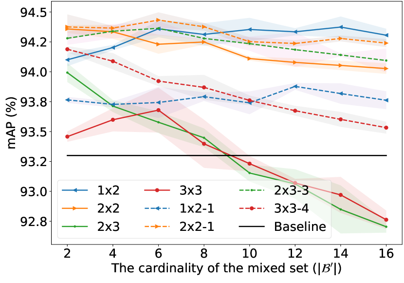
Figure 10: Comparisons of various grid settings on mAP metric. The mean in a solid or dash line and standard deviation in shaded region are given. Each solid-dash pair in the same color is a grid setting without and with dropout.

V Conclusion

In this paper, we introduce a simple but effective augmentation strategy, namely SpliceMix, for multi-label image classification. SpliceMix augments the sample space and batch scale simultaneously. In augmented sample space, mixed images with semantic blending contribute to alleviating co-occurred bias. In augmented batch, the splice of regular images and mixed images enables cross-scale training and consistency learning. Hence, we also offer a non-parametric, consistency learning-based extension (SpliceMix-CL) to present the flexible extensibility of our SpliceMix. Extensive experiments on various tasks demonstrate the effectiveness of the proposed methods.

References

- [1] K. He, X. Zhang, S. Ren, and J. Sun, “Deep residual learning for image recognition,” in Proc. IEEE Conf. Comput. Vis. Pattern Recognit., 2016, pp. 770–778.
- [2] J. Mellor, J. Turner, A. Storkey, and E. J. Crowley, “Neural architecture search without training,” in Proc. Int. Conf. Mach. Learn. PMLR, 2021, pp. 7588–7598.
- [3] H. Zhang, M. Cisse, Y. N. Dauphin, and D. Lopez-Paz, “Mixup: Beyond empirical risk minimization,” in Proc. Int. Conf. Learn. Representations, 2018.
- [4] B. Li, F. Zhang, L. Wang, Y. Wang, T. Liu, Z. Lin, W. An, and Y. Guo, “Ddaug: Differentiable data augmentation for weakly supervised semantic segmentation,” IEEE Trans. Multimedia, pp. 1–12, 2023.
- [5] K. He, X. Chen, S. Xie, Y. Li, P. Dollár, and R. Girshick, “Masked autoencoders are scalable vision learners,” in Proc. IEEE Conf. Comput. Vis. Pattern Recognit., 2022, pp. 16 000–16 009.
- [6] X. Yang, F. Liu, and G. Lin, “Effective end-to-end vision language pretraining with semantic visual loss,” IEEE Trans. Multimedia, no. 99, pp. 1–10, 2023.
- [7] K. Zhu and J. Wu, “Residual attention: A simple but effective method for multi-label recognition,” in Proc. IEEE Int. Conf. Comput. Vis., 2021, pp. 184–193.
- [8] R. Liu, H. Liu, G. Li, H. Hou, T. Yu, and T. Yang, “Contextual debiasing for visual recognition with causal mechanisms,” in Proc. IEEE Conf. Comput. Vis. Pattern Recognit., 2022, pp. 12 755–12 765.
- [9] R. You, Z. Guo, L. Cui, X. Long, Y. Bao, and S. Wen, “Cross-modality attention with semantic graph embedding for multi-label classification,” in Proc. AAAI Conf. Artif. Intell., vol. 34, no. 07, 2020, pp. 12 709–12 716.
- [10] S. Yun, D. Han, S. J. Oh, S. Chun, J. Choe, and Y. Yoo, “Cutmix: Regularization strategy to train strong classifiers with localizable features,” in Proc. IEEE Int. Conf. Comput. Vis., 2019, pp. 6023–6032.
- [11] E. Hoffer, T. Ben-Nun, I. Hubara, N. Giladi, T. Hoefler, and D. Soudry, “Augment your batch: Improving generalization through instance repetition,” in Proc. IEEE Conf. Comput. Vis. Pattern Recognit., 2020, pp. 8129–8138.
- [12] J. Ye, J. He, X. Peng, W. Wu, and Y. Qiao, “Attention-driven dynamic graph convolutional network for multi-label image recognition,” in Proc. Eur. Conf. Comput. Vis. Springer, 2020, pp. 649–665.
- [13] Z.-M. Chen, X.-S. Wei, P. Wang, and Y. Guo, “Multi-label image recognition with graph convolutional networks,” in Proc. IEEE Conf. Comput. Vis. Pattern Recognit., 2019, pp. 5177–5186.
- [14] J. Lanchantin, T. Wang, V. Ordonez, and Y. Qi, “General multi-label image classification with transformers,” in Proc. IEEE Conf. Comput. Vis. Pattern Recognit., 2021, pp. 16 478–16 488.
- [15] X. Deng, S. Feng, G. Lyu, T. Wang, and C. Lang, “Beyond word embeddings: Heterogeneous prior knowledge driven multi-label image classification,” IEEE Trans. Multimedia, 2022.
- [16] W. Zhou, W. Jiang, D. Chen, H. Hu, and T. Su, “Mining semantic information with dual relation graph network for multi-label image classification,” IEEE Trans. Multimedia, 2023.
- [17] K. K. Singh, D. Mahajan, K. Grauman, Y. J. Lee, M. Feiszli, and D. Ghadiyaram, “Don’t judge an object by its context: learning to overcome contextual bias,” in Proc. IEEE Conf. Comput. Vis. Pattern Recognit., 2020, pp. 11 070–11 078.
- [18] J.-H. Kim, W. Choo, and H. O. Song, “Puzzle mix: Exploiting saliency and local statistics for optimal mixup,” in Proc. Int. Conf. Mach. Learn. PMLR, 2020, pp. 5275–5285.
- [19] J. Liu, B. Liu, H. Zhou, H. Li, and Y. Liu, “Tokenmix: Rethinking image mixing for data augmentation in vision transformers,” in Proc. Eur. Conf. Comput. Vis. Springer, 2022, pp. 455–471.
- [20] V. Olsson, W. Tranheden, J. Pinto, and L. Svensson, “Classmix: Segmentation-based data augmentation for semi-supervised learning,” in Proc. IEEE Winter Conf. Appl. Comput. Vis., 2021, pp. 1369–1378.
- [21] Y. Su, R. Sun, G. Lin, and Q. Wu, “Context decoupling augmentation for weakly supervised semantic segmentation,” in Proc. IEEE Int. Conf. Comput. Vis., 2021, pp. 7004–7014.
- [22] A. S. Uddin, M. S. Monira, W. Shin, T. Chung, and S.-H. Bae, “Saliencymix: A saliency guided data augmentation strategy for better regularization,” in Proc. Int. Conf. Learn. Representations, 2021.
- [23] F. Zhu, H. Li, W. Ouyang, N. Yu, and X. Wang, “Learning spatial regularization with image-level supervisions for multi-label image classification,” in Proc. IEEE Conf. Comput. Vis. Pattern Recognit., 2017, pp. 5513–5522.
- [24] T. Chen, Z. Wang, G. Li, and L. Lin, “Recurrent attentional reinforcement learning for multi-label image recognition,” in Proc. AAAI Conf. Artif. Intell., vol. 32, no. 1, 2018.
- [25] B.-B. Gao and H.-Y. Zhou, “Learning to discover multi-class attentional regions for multi-label image recognition,” IEEE Trans. Image Process., vol. 30, pp. 5920–5932, 2021.
- [26] J. Zhan, J. Liu, W. Tang, G. Jiang, X. Wang, B.-B. Gao, T. Zhang, W. Wu, W. Zhang, C. Wang et al., “Global meets local: Effective multi-label image classification via category-aware weak supervision,” in Proc. ACM Int. Conf. Multimedia, 2022, pp. 6318–6326.
- [27] W. Zaremba, I. Sutskever, and O. Vinyals, “Recurrent neural network regularization,” arXiv preprint arXiv:1409.2329, 2014.
- [28] T. N. Kipf and M. Welling, “Semi-supervised classification with graph convolutional networks,” arXiv preprint arXiv:1609.02907, 2016.
- [29] A. Vaswani, N. Shazeer, N. Parmar, J. Uszkoreit, L. Jones, A. N. Gomez, Ł. Kaiser, and I. Polosukhin, “Attention is all you need,” in Proc. Adv. Neural Inf. Process. Syst., vol. 30, 2017.
- [30] J. Wang, Y. Yang, J. Mao, Z. Huang, C. Huang, and W. Xu, “Cnn-rnn: A unified framework for multi-label image classification,” in Proc. IEEE Conf. Comput. Vis. Pattern Recognit., 2016, pp. 2285–2294.
- [31] S. Narayan, A. Gupta, S. Khan, F. S. Khan, L. Shao, and M. Shah, “Discriminative region-based multi-label zero-shot learning,” in Proc. IEEE Int. Conf. Comput. Vis., 2021, pp. 8731–8740.
- [32] T. Chen, M. Xu, X. Hui, H. Wu, and L. Lin, “Learning semantic-specific graph representation for multi-label image recognition,” in Proc. IEEE Int. Conf. Comput. Vis., 2019, pp. 522–531.
- [33] J. Zhao, K. Yan, Y. Zhao, X. Guo, F. Huang, and J. Li, “Transformer-based dual relation graph for multi-label image recognition,” in Proc. IEEE Int. Conf. Comput. Vis., 2021, pp. 163–172.
- [34] S. Liu, L. Zhang, X. Yang, H. Su, and J. Zhu, “Query2label: A simple transformer way to multi-label classification,” arXiv preprint arXiv:2107.10834, 2021.
- [35] X. Zhu, J. Cao, J. Ge, W. Liu, and B. Liu, “Two-stream transformer for multi-label image classification,” in Proc. ACM Int. Conf. Multimedia, 2022, pp. 3598–3607.
- [36] R. Liu, J. Huang, G. Li, and T. H. Li, “Causality compensated attention for contextual biased visual recognition,” in Proc. Int. Conf. Learn. Representations, 2023.
- [37] J. Yoo, N. Ahn, and K.-A. Sohn, “Rethinking data augmentation for image super-resolution: A comprehensive analysis and a new strategy,” in Proc. IEEE Conf. Comput. Vis. Pattern Recognit., 2020, pp. 8375–8384.
- [38] T. DeVries and G. W. Taylor, “Improved regularization of convolutional neural networks with cutout,” arXiv preprint arXiv:1708.04552, 2017.
- [39] J.-H. Lee, M. Z. Zaheer, M. Astrid, and S.-I. Lee, “Smoothmix: A simple yet effective data augmentation to train robust classifiers,” in Proc. IEEE Conf. Comput. Vis. Pattern Recognit. Workshops, 2020, pp. 756–757.
- [40] D. Walawalkar, Z. Shen, Z. Liu, and M. Savvides, “Attentive cutmix: An enhanced data augmentation approach for deep learning based image classification,” arXiv preprint arXiv:2003.13048, 2020.
- [41] S. Fort, A. Brock, R. Pascanu, S. De, and S. L. Smith, “Drawing multiple augmentation samples per image during training efficiently decreases test error,” arXiv preprint arXiv:2105.13343, 2021.
- [42] J. Redmon and A. Farhadi, “Yolov3: An incremental improvement,” arXiv preprint arXiv:1804.02767, 2018.
- [43] A. Paszke, S. Gross, F. Massa, A. Lerer, J. Bradbury, G. Chanan, T. Killeen, Z. Lin, N. Gimelshein, L. Antiga et al., “Pytorch: An imperative style, high-performance deep learning library,” in Proc. Adv. Neural Inf. Process. Syst., vol. 32, 2019.
- [44] Y. Zhang, T. Xiang, T. M. Hospedales, and H. Lu, “Deep mutual learning,” in Proc. IEEE Conf. Comput. Vis. Pattern Recognit., 2018, pp. 4320–4328.
- [45] B. Zhao, Q. Cui, R. Song, Y. Qiu, and J. Liang, “Decoupled knowledge distillation,” in Proc. IEEE Conf. Comput. Vis. Pattern Recognit., 2022, pp. 11 953–11 962.
- [46] D. Chen, J.-P. Mei, Y. Zhang, C. Wang, Z. Wang, Y. Feng, and C. Chen, “Cross-layer distillation with semantic calibration,” in Proc. AAAI Conf. Artif. Intell., vol. 35, no. 8, 2021, pp. 7028–7036.
- [47] J. Gou, B. Yu, S. J. Maybank, and D. Tao, “Knowledge distillation: A survey,” Int. J. Comput. Vis., vol. 129, no. 6, pp. 1789–1819, 2021.
- [48] T. Ridnik, E. Ben-Baruch, N. Zamir, A. Noy, I. Friedman, M. Protter, and L. Zelnik-Manor, “Asymmetric loss for multi-label classification,” in Proc. IEEE Int. Conf. Comput. Vis., 2021, pp. 82–91.
- [49] G. Hinton, O. Vinyals, J. Dean et al., “Distilling the knowledge in a neural network,” arXiv preprint arXiv:1503.02531, vol. 2, no. 7, 2015.
- [50] Z. Liu, H. Mao, C.-Y. Wu, C. Feichtenhofer, T. Darrell, and S. Xie, “A convnet for the 2020s,” in Proc. IEEE Conf. Comput. Vis. Pattern Recognit., 2022, pp. 11 976–11 986.
- [51] T.-Y. Lin, M. Maire, S. Belongie, J. Hays, P. Perona, D. Ramanan, P. Dollár, and C. L. Zitnick, “Microsoft coco: Common objects in context,” in Proc. Eur. Conf. Comput. Vis. Springer, 2014, pp. 740–755.
- [52] F. Zhou, S. Huang, and Y. Xing, “Deep semantic dictionary learning for multi-label image classification,” in Proc. AAAI Conf. Artif. Intell., vol. 35, no. 4, 2021, pp. 3572–3580.
- [53] Z.-M. Chen, Q. Cui, B. Zhao, R. Song, X. Zhang, and O. Yoshie, “Sst: Spatial and semantic transformers for multi-label image recognition,” IEEE Trans. Image Process., vol. 31, pp. 2570–2583, 2022.
- [54] J. Qin, J. Fang, Q. Zhang, W. Liu, X. Wang, and X. Wang, “Resizemix: Mixing data with preserved object information and true labels,” arXiv preprint arXiv:2012.11101, 2020.
- [55] L. Yang, X. Li, B. Zhao, R. Song, and J. Yang, “Recursivemix: Mixed learning with history,” in Proc. Adv. Neural Inf. Process. Syst., vol. 35, 2022, pp. 8427–8440.
- [56] M. Everingham, L. Van Gool, C. K. Williams, J. Winn, and A. Zisserman, “The pascal visual object classes (voc) challenge,” Int. J. Comput. Vis., vol. 88, no. 2, pp. 303–338, 2010.
- [57] O. Russakovsky, J. Deng, H. Su, J. Krause, S. Satheesh, S. Ma, Z. Huang, A. Karpathy, A. Khosla, M. Bernstein et al., “Imagenet large scale visual recognition challenge,” Int. J. Comput. Vis., vol. 115, no. 3, pp. 211–252, 2015.
- [58] T. Chen, T. Pu, H. Wu, Y. Xie, and L. Lin, “Structured semantic transfer for multi-label recognition with partial labels,” in Proc. AAAI Conf. Artif. Intell., vol. 36, no. 1, 2022, pp. 339–346.
- [59] Y. Zhang, Y. Cheng, X. Huang, F. Wen, R. Feng, Y. Li, and Y. Guo, “Simple and robust loss design for multi-label learning with missing labels,” arXiv preprint arXiv:2112.07368, 2021.
- [60] E. Cole, O. Mac Aodha, T. Lorieul, P. Perona, D. Morris, and N. Jojic, “Multi-label learning from single positive labels,” in Proc. IEEE Conf. Comput. Vis. Pattern Recognit., 2021, pp. 933–942.
- [61] T.-Y. Lin, P. Goyal, R. Girshick, K. He, and P. Dollár, “Focal loss for dense object detection,” in Proc. IEEE Int. Conf. Comput. Vis., 2017, pp. 2980–2988.
- [62] N. Ma, X. Zhang, H.-T. Zheng, and J. Sun, “Shufflenet v2: Practical guidelines for efficient cnn architecture design,” in Proc. Eur. Conf. Comput. Vis., 2018, pp. 116–131.
- [63] A. Dosovitskiy, L. Beyer, A. Kolesnikov, D. Weissenborn, X. Zhai, T. Unterthiner, M. Dehghani, M. Minderer, G. Heigold, S. Gelly et al., “An image is worth 16x16 words: Transformers for image recognition at scale,” arXiv preprint arXiv:2010.11929, 2020.
- [64] Z. Liu, Y. Lin, Y. Cao, H. Hu, Y. Wei, Z. Zhang, S. Lin, and B. Guo, “Swin transformer: Hierarchical vision transformer using shifted windows,” in Proc. IEEE Int. Conf. Comput. Vis., 2021, pp. 10 012–10 022.
- [65] M. Singh, L. Gustafson, A. Adcock, V. de Freitas Reis, B. Gedik, R. P. Kosaraju, D. Mahajan, R. Girshick, P. Dollár, and L. Van Der Maaten, “Revisiting weakly supervised pre-training of visual perception models,” in Proc. IEEE Conf. Comput. Vis. Pattern Recognit., 2022, pp. 804–814.
- [66] T. Ridnik, E. Ben-Baruch, A. Noy, and L. Zelnik-Manor, “Imagenet-21k pretraining for the masses,” arXiv preprint arXiv:2104.10972, 2021.
- [67] H. Touvron, A. Vedaldi, M. Douze, and H. Jégou, “Fixing the train-test resolution discrepancy,” in Proc. Adv. Neural Inf. Process. Syst., vol. 32, 2019.
- [68] H. Caesar, J. Uijlings, and V. Ferrari, “Coco-stuff: Thing and stuff classes in context,” in Proc. IEEE Conf. Comput. Vis. Pattern Recognit., 2018, pp. 1209–1218.
- [69] S. S. Kim, S. Zhang, N. Meister, and O. Russakovsky, “[re] don’t judge an object by its context: learning to overcome contextual bias,” arXiv preprint arXiv:2104.13582, 2021.
- [70] B. Zhou, A. Khosla, A. Lapedriza, A. Oliva, and A. Torralba, “Learning deep features for discriminative localization,” in Proc. IEEE Conf. Comput. Vis. Pattern Recognit., 2016, pp. 2921–2929.