Mixing Classifiers to Alleviate the Accuracy-Robustness Trade-Off

Abstract

Deep learning classifiers have recently found tremendous success in data-driven control systems. However, standard learning models often suffer from an accuracy-robustness trade-off, which is a limitation that must be overcome in the control of safety-critical systems that require both high performance and rigorous robustness guarantees. In this work, we build upon the recent “locally biased smoothing” method to develop classifiers that simultaneously inherit high accuracy from standard models and high robustness from robust models. Specifically, we extend locally biased smoothing to the multi-class setting, and then overcome its performance bottleneck by generalizing the formulation to “mix” the outputs of a standard neural network and a robust neural network. Both models are pre-trained, and thus our method does not require additional training. We prove that when the robustness of the robust base model is certifiable, no alteration or attack within a closed-form $\ell_{p}$ radius on an input can result in misclassification of the mixed classifier; the proposed model inherits the certified robustness. Moreover, we use numerical experiments on the CIFAR-10 benchmark dataset to verify that the mixed model noticeably improves the accuracy-robustness trade-off.

I Introduction

In recent years, high-performing machine learning models have been successfully employed in a range of control settings, including reinforcement learning for dynamical systems with uncertainty [1, 2] and self-driving cars [3, 4]. However, models such as neural networks have been shown to be vulnerable to adversarial attacks, which are imperceptibly small input data alterations maliciously designed to cause failure [5, 6, 7]. For example, both digital and physical attacks on traffic signs have successfully fooled state-of-the-art image classifiers [8, 9]. This vulnerability makes such models unreliable for safety-critical control where guaranteeing robustness is necessary. In response, “adversarial training (AT)” [10, 11, 12, 13, 14] has been studied to alleviate the susceptibility. AT builds robust neural networks by training on adversarially attacked data.

A parallel line of work focuses on certified (that is, mathematical proof of) robustness [15, 16, 17]. Among the most popular of these methods, “randomized smoothing (RS)” seeks to achieve certified robustness by processing intentionally corrupted data at test time [18, 19, 20]. RS has recently been applied to robustify reinforcement learning-based control strategies [21, 22]. The recent work [23] has shown that a “locally biased smoothing” method, which robustifies the model locally based on the particular test datum, outperforms the traditional data-agnostic RS that uses globally fixed smoothing noise. However, [23] only focuses on binary classification problems, significantly limiting the applications. Moreover, [23] relies on the robustness of a $K$-nearest-neighbor ($K$-NN) classifier, which suffers from the lack of representation power when applied to harder problems and becomes a performance bottleneck.

While some works have shown that there exists a fundamental trade-off between accuracy and robustness [24, 25], recent research has argued that it should be possible to simultaneously achieve robustness and accuracy on benchmark datasets [26]. To this end, variants of AT that improve the accuracy-robustness trade-off have been proposed, including TRADES [25], Interpolated Adversarial Training [27], and many others [28, 29, 30, 31]. However, even with these improvements, degraded clean accuracy is often an inevitable price of achieving robustness. Moreover, standard non-robust models often achieve enormous performance gains by pre-training on larger datasets, whereas the effect of pre-training on robust classifiers is less understood and may be less prominent [32, 33].

This work makes a theoretically disciplined step towards robustifying models without sacrificing clean accuracy. Specifically, we build upon locally biased smoothing and replace its underlying $K$-NN classifier with a robust neural network that can be obtained via various existing methods. We also modify how the standard and robust models are “mixed” accordingly. The resulting formulation, to be introduced formally in Section III, is a convex combination of the output of a standard neural network and the output of a robust neural network. We prove that, when the robust neural network has a bounded Lipschitz constant or is built via RS, the mixed classifier also has a closed-form certified robust radius. More importantly, the proposed method achieves an empirical robustness level close to that of the robust base model while approaching the clean accuracy of the standard base classifier. This desirable behavior significantly improves the accuracy-robustness trade-off for tasks where standard models noticeably outperform robust models on clean data.

Note that we do not make any assumptions about how the standard and robust base models are obtained (can be AT, RS, or others), nor do we make assumptions on the adversarial attack type and budget. Thus, our mixed classification scheme can take advantage of pre-training on large datasets via the standard base classifier and benefit from ever-improving robust training methods via the robust base classifier.

II Background and related works

II-A Notations

The $\ell_{p}$ norm is denoted by $\lVert\cdot\rVert_{p}$, while $\lVert\cdot\rVert_{p*}$ denotes its dual norm. The matrix $I_{d}$ denotes the identity matrix in ${\mathbb{R}}^{d\times d}$. For a scalar $a$, $\operatorname{sgn}(a)\in\{-1,0,1\}$ denotes its sign. For a natural number $c$, the set $[c]$ is defined as $\{1,2,\dots,c\}$. For an event $A$, the indicator function ${\mathbb{I}}(A)$ evaluates to 1 if $A$ takes place and 0 otherwise. The notation ${\mathbb{P}}_{X\sim{\mathcal{S}}}[A(X)]$ denotes the probability for an event $A(X)$ to occur, where $X$ is a random variable drawn from the distribution ${\mathcal{S}}$. The normal distribution on ${\mathbb{R}}^{d}$ with mean $\overline{x}$ and covariance $\Sigma$ is written as ${\mathcal{N}}(\overline{x},\Sigma)$. We denote the cumulative distribution function of ${\mathcal{N}}(0,1)$ on ${\mathbb{R}}$ by $\Phi$ and write its inverse function as $\Phi^{-1}$.

Consider a model $g:{\mathbb{R}}^{d}\to{\mathbb{R}}^{c}$, whose components are $g_{i}:{\mathbb{R}}^{d}\to{\mathbb{R}},\ i\in[c]$, where $d$ is the dimension of the input and $c$ is the number of classes. In this paper, we assume that $g(\cdot)$ does not have the desired level of robustness, and refer to it as a “standard model”, as opposed to a “robust model” which we denote as $h(\cdot)$. We consider $\ell_{p}$ norm-bounded attacks on differentiable neural networks. A classifier $f:{\mathbb{R}}^{d}\to[c]$, defined as $f(x)=\operatorname*{arg\,max}_{i\in[c]}g_{i}(x)$, is considered robust against adversarial attacks at an input datum $x\in{\mathbb{R}}^{d}$ if it assigns the same class to all perturbed inputs $x+\delta$ such that $\lVert\delta\rVert_{p}\leq\epsilon$, where $\epsilon\geq 0$ is the attack radius.

II-B Related Adversarial Attacks and Defenses

The fast gradient sign method (FGSM) and projected gradient descent (PGD) attacks based on differentiating the cross-entropy loss have been considered the most classic and straightforward attacks [34, 11]. However, they have been shown to be too weak, as defenses that are only designed against these attacks can be easily circumvented [35, 36, 37]. To this end, various attack methods based on alternative loss functions, Expectation Over Transformation, and black-box perturbations have been proposed. Such efforts include AutoAttack [38], adaptive attack [39], and many others.

On the defense side, while AT [34] and TRADES [25] have seen enormous success, such methods are often limited by a significantly larger amount of required training data [40] and a decrease in generalization capability. Initiatives that construct more effective training data via data augmentation [41, 42] and generative models [43] have successfully produced more robust models. Improved versions of AT [44, 45] have also been proposed.

Previous initiatives that aim to enhance the accuracy-robustness trade-off include using alternative attacks during training [46], appending early-exit side branches to a single network [47], and applying AT for regularization [48]. Moreover, ensemble-based defenses, such as random ensemble [49] and diverse ensemble [50, 51], have been proposed. In comparison, this work considers two separate classifiers and uses their synergy to improve the accuracy-robustness trade-off, achieving higher performances.

II-C Locally Biased Smoothing

Randomized smoothing, popularized by [18], achieves robustness at test time by replacing $f(x)=\operatorname*{arg\,max}_{i\in[c]}g_{i}(x)$ with a smoothed classifier $\widetilde{f}(x)=\operatorname*{arg\,max}_{i\in[c]}\mathbb{E}_{\xi\sim{\mathcal{S}}}\left[g(x+\xi)\right]$, where ${\mathcal{S}}$ is a smoothing distribution. A common choice for ${\mathcal{S}}$ is a Gaussian distribution.

The authors of [23] have recently argued that data-invariant RS does not always achieve robustness. They have shown that in the binary classification setting, RS with an unbiased distribution is suboptimal, and an optimal smoothing procedure shifts the input point in the direction of its true class. Since the true class is generally unavailable, a “direction oracle” is used as a surrogate. This “locally biased smoothing” method is no longer randomized and outperforms traditional data-blind RS. The locally biased smoothed classifier, denoted $h^{\gamma}\colon{\mathbb{R}}^{d}\to{\mathbb{R}}$, is obtained via the deterministic calculation

$$h^{\gamma}(x)=g(x)+\gamma h(x)\lVert\nabla g(x)\rVert_{p*},$$

where $h(x)\in\{-1,1\}$ is the direction oracle and $\gamma\geq 0$ is a trade-off parameter. The direction oracle should come from an inherently robust classifier (which is often less accurate). In [23], this direction oracle is chosen to be a one-nearest-neighbor classifier.

III Using a Robust Neural Network as the Smoothing Oracle

Since locally biased smoothing was designed for binary classification problems, we first extend it to the multi-class setting. To achieve this, we treat the output $h^{\gamma}_{i}(x)$ of each class independently, giving rise to:

$$h_{\text{smo1},i}^{\gamma}(x)\coloneqq g_{i}(x)+\gamma h_{i}(x)\lVert\nabla g_{i}(x)\rVert_{p*},\;\;\;i\in[c].$$ (1)

Note that if $\lVert\nabla g_{i}(x)\rVert_{p*}$ is large for some $i$, then $h_{\text{smo1},i}^{\gamma}(x)$ can be large even if both $g_{i}(x)$ and $h_{i}(x)$ are small, potentially leading to incorrect predictions. To remove the effect of the magnitude difference across the classes, we propose a normalized formulation as follows:

$$h_{\text{smo2},i}^{\gamma}(x)\coloneqq\frac{g_{i}(x)+\gamma h_{i}(x)\lVert\nabla g_{i}(x)\rVert_{p*}}{1+\gamma\lVert\nabla g_{i}(x)\rVert_{p*}},\;\;\;i\in[c].$$ (2)

The parameter $\gamma$ adjusts the trade-off between clean accuracy and robustness. When $\gamma=0$, it holds that $h_{\text{smo2},i}^{\gamma}(x)\equiv g_{i}(x)$ for all $i$. When $\gamma\to\infty$, it holds that $h_{\text{smo2},i}^{\gamma}(x)\to h_{i}(x)$ for all $x$ and all $i$.

With the mixing procedure generalized to the multi-class setting, we now discuss the choice of the smoothing oracle $h_{i}(\cdot)$. While $K$-NN classifiers are relatively robust and can be used as the oracle, their representation power is too weak. On the CIFAR-10 image classification task [52], $K$-NN only achieves around $35\%$ accuracy on clean test data. In contrast, an adversarially trained ResNet can reach $50\%$ accuracy on attacked test data [34]. This lackluster performance of $K$-NN becomes a significant bottleneck in the accuracy-robustness trade-off of the mixed classifier. To this end, we replace the $K$-NN model with a robust neural network. The robustness of this network can be achieved via various methods, including AT, TRADES, and RS.

Further scrutinizing Eq. 2 leads to the question of whether $\lVert\nabla g_{i}(x)\rVert_{p*}$ is the best choice for adjusting the mixture of $g(\cdot)$ and $h(\cdot)$. In fact, this gradient magnitude term is a result of the assumption that $h(x)\in\{-1,1\}$, which is the setting considered in [23]. Here, we no longer have this assumption. Instead, we assume both $g(\cdot)$ and $h(\cdot)$ to be differentiable. Thus, we further generalize the formulation to

$$h_{\text{smo3},i}^{\gamma}(x)\coloneqq\frac{g_{i}(x)+\gamma R_{i}(x)h_{i}(x)}{1+\gamma R_{i}(x)},\;\;\;i\in[c],$$ (3)

where $R_{i}(x)$ is an extra scalar term that can potentially depend on both $\nabla g_{i}(x)$ and $\nabla h_{i}(x)$ to determine the “trustworthiness” of the base classifiers. Here, we empirically compare four options for $R_{i}(x)$, namely, $1$, $\lVert\nabla g_{i}(x)\rVert_{p*}$, $\lVert\nabla\max_{j}g_{j}(x)\rVert_{p*}$, and $\frac{\lVert\nabla g_{i}(x)\rVert_{p*}}{\lVert\nabla h_{i}(x)\rVert_{p*}}$.

Another design question is whether $g(\cdot)$ and $h(\cdot)$ should be the pre-softmax logits or the post-softmax probabilities. Note that since most attack methods are designed based on the logits, incorporating the softmax function into the model may result in gradient masking, an undesirable phenomenon that makes it hard to properly evaluate the proposed method. Thus, we have the following two options that make the mixed model compatible with existing gradient-based attacks:

1. Use the logits for both $g(\cdot)$ and $h(\cdot)$.

2. Use the probabilities for both $g(\cdot)$ and $h(\cdot)$, and then convert the mixed probabilities back to logits. The required “inverse-softmax” operator is given simply by the natural logarithm, and does not change the prediction.

In Fig. 1, we compare the different choices for $R_{i}(x)$ by visualizing the accuracy-robustness trade-off. Based on this “clean accuracy versus PGD₁₀-attacked accuracy” plot, where PGD_T denotes $T$-step PGD, we conclude that $R_{i}(x)=1$ gives the best accuracy-robustness trade-off, and $g(\cdot)$ and $h(\cdot)$ should be the probabilities.

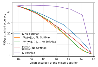
Figure 1: Comparing the “attacked accuracy versus clean accuracy” curve for various options for $R_{i}(x)$. “Softmax” represents the formulation that use the probabilities for $g(\cdot)$ and $h(\cdot)$ followed by a natural log on the assembled $h_{\text{smo3},i}^{\gamma}(\cdot)$.

In later sections, we will offer additional theoretical and empirical justifications for this choice. Specifically, in addition to the set of base classifiers (a pair of standard and adversarially-trained ResNet18s) considered in Fig. 1, we provide examples in Section IV-C using alternative model architectures, different methods to train the robust base classifiers, and various attack budgets, all of which lead to the same best choice for $R_{i}(x)$. With these design choices implemented, the formulation Eq. 3 can be re-parameterized as

$$h_{i}^{\alpha}(x)\coloneqq\log\big{(}(1-\alpha)g_{i}(x)+\alpha h_{i}(x)\big{)},\;\;i\in[c],$$ (4)

where $\alpha=\frac{\gamma}{1+\gamma}\in[0,1]$. We take $h^{\alpha}(\cdot)$ in Eq. 4, which outputs the natural logarithm of a convex combination of the probabilities $g(\cdot)$ and $h(\cdot)$, as our proposed mixed classifier.

III-A Theoretical Certified Robust Radius

In this section, we derive certified robust radii for $h^{\alpha}(\cdot)$ introduced in Eq. 4, given in terms of the robustness properties of $h(\cdot)$ and the mixing parameter $\alpha$. The results ensure that despite being more sophisticated than a single model, $h^{\alpha}(\cdot)$ cannot be easily conquered, even if an adversary attempts to adapt its attack methods to its structure. Such guarantees are of paramount importance for reliable deployment in safety-critical control applications. Since we use probabilities for $g(\cdot)$ and $h(\cdot)$, it holds that $0\leq g_{i}(\cdot)\leq 1$ and $0\leq h_{i}(\cdot)\leq 1$ for all $i$. To facilitate the proofs, we introduce the following generalized notion of certified robustness.

Definition 1.

Consider an arbitrary input $x\in{\mathbb{R}}^{d}$ and let $y=\operatorname*{arg\,max}_{i}h_{i}(x)$, $\mu\in[0,1]$, and $r\geq 0$. Then, $h(\cdot)$ is said to be certifiably robust at $x$ with margin $\mu$ and radius $r$ if $h_{y}(x+\delta)\geq h_{i}(x+\delta)+\mu$ for all $i\neq y$ and all $\delta\in{\mathbb{R}}^{d}$ such that $\lVert\delta\rVert_{p}\leq r$.

Lemma 1.

Let $x\in{\mathbb{R}}^{d}$ and $r\geq 0$. If it holds that $\alpha\in[\frac{1}{2},1]$ and $h(\cdot)$ is certifiably robust at $x$ with margin $\frac{1-\alpha}{\alpha}$ and radius $r$, then the mixed classifier $h^{\alpha}(\cdot)$ is robust in the sense that $\operatorname*{arg\,max}_{i}h_{i}^{\alpha}(x+\delta)=\operatorname*{arg\,max}_{i}h_{i}(x)$ for all $\delta\in{\mathbb{R}}^{d}$ such that $\lVert\delta\rVert_{p}\leq r$.

Proof.

Suppose that $h(\cdot)$ is certifiably robust at $x$ with margin $\frac{1-\alpha}{\alpha}$ and radius $r$. Since $\alpha\in[\frac{1}{2},1]$, it holds that $\frac{1-\alpha}{\alpha}\in[0,1]$. Let $y=\operatorname*{arg\,max}_{i}h_{i}(x)$. Consider an arbitrary $i\in[c]\setminus\{y\}$ and $\delta\in{\mathbb{R}}^{d}$ such that $\lVert\delta\rVert_{p}\leq r$. Since $g_{i}(x+\delta)\in[0,1]$, it holds that

$$\exp\left(h_{y}^{\alpha}(x+\delta)\right)-\exp\left(h_{i}^{\alpha}(x+\delta)\right)$$

$$\qquad=(1-\alpha)(g_{y}(x+\delta)-g_{i}(x+\delta))$$

$$\hskip 44.95535pt+\alpha(h_{y}(x+\delta)-h_{i}(x+\delta))$$

$$\qquad\geq(1-\alpha)(0-1)+\alpha(h_{y}(x+\delta)-h_{i}(x+\delta))$$

$$\qquad\geq(\alpha-1)+\alpha\left(\tfrac{1-\alpha}{\alpha}\right)=0.$$

Thus, it holds that $h_{y}^{\alpha}(x+\delta)\geq h_{i}^{\alpha}(x+\delta)$ for all $i\neq y$, and thus $\operatorname*{arg\,max}_{i}h_{i}^{\alpha}(x+\delta)=y=\operatorname*{arg\,max}_{i}h_{i}(x)$. ∎

Lemma 1 provides further justifications for using probabilities instead of logits in the mixing operation. Intuitively, it holds that $(1-\alpha)g_{i}(\cdot)$ is bounded between $0$ and $1-\alpha$, so as long as $\alpha$ is relatively large (specifically, at least $\frac{1}{2}$), the detrimental effect of $g(\cdot)$ when subject to attack can be overcome by $h(\cdot)$. On the other hand, if each $g_{i}(\cdot)$ is the logit, then it cannot be bounded, and thus it is much harder to overcome its vulnerability.

Since we do not make assumptions on the Lipschitzness or robustness of $g(\cdot)$, Lemma 1 is tight. To understand this, we suppose that there exists some $i\in[c]\backslash\{y\}$ and $\delta\neq 0$ such that $\lVert\delta\rVert_{p}\leq r$ that make $h_{y}(x+\delta)-h_{i}(x+\delta)\coloneqq h_{d}$ smaller than $\frac{1-\alpha}{\alpha}$, indicating that $-\alpha h_{d}>\alpha-1$. Since the only information about $g(\cdot)$ is that $g_{i}(x+\delta)\in[0,1]$ and thus the value $g_{y}(x+\delta)-g_{i}(x+\delta)$ can be any number in $[-1,1]$, it is possible that $(1-\alpha)\left(g_{y}(x+\delta)-g_{i}(x+\delta)\right)$ is smaller than $-\alpha h_{d}$. In this case, it holds that $h_{y}^{\alpha}(x+\delta)<h_{i}^{\alpha}(x+\delta)$, and thus $\operatorname*{arg\,max}_{i}h_{i}^{\alpha}(x+\delta)\neq\operatorname*{arg\,max}_{i}h_{i}(x)$.

While most certifiably robust models consider the special case where the margin is zero, we will show that models built via common methods are also robust with non-zero margins, and can thus take advantage of Lemma 1. Specifically, we consider two types of popular robust classifiers: Lipschitz continuous models (Theorem 1) and RS models (Theorem 2).

Definition 2.

A function $f\colon{\mathbb{R}}^{d}\to{\mathbb{R}}$ is called $\ell_{p}$-Lipschitz continuous if there exists $L\in(0,\infty)$ such that $|f(x^{\prime})-f(x)|\leq L\|x^{\prime}-x\|_{p}$ for all $x^{\prime},x\in{\mathbb{R}}^{d}$. The Lipschitz constant of such $f$ is defined to be $\operatorname{Lip}_{p}(f)\coloneqq\inf\{L\in(0,\infty):|f(x^{\prime})-f(x)|\leq L\|x^{\prime}-x\|_{p}\leavevmode\nobreak\ \text{for all $x^{\prime},x\in{\mathbb{R}}^{d}$}\}$.

Assumption 1.

The classifier $h(\cdot)$ is robust in the sense that, for all $i\in\{1,2,\dots,n\}$, $h_{i}(\cdot)$ is $\ell_{p}$-Lipschitz continuous with Lipschitz constant $\operatorname{Lip}_{p}(h_{i})$.

Assumption 1 is not restrictive in practice. For example, RS with Gaussian smoothing variance $\sigma^{2}I_{d}$ on the input yields robust models with $\ell_{2}$-Lipschitz constant $\sqrt{\frac{2}{\pi\sigma^{2}}}$ [53]. Moreover, empirically robust methods such as TRADES and AT often train Lipschitz continuous models, even though evaluating their closed-form Lipschitz constants can be hard.

Theorem 1.

Suppose that Assumption 1 holds, and let $x\in{\mathbb{R}}^{d}$ be arbitrary. Let $y=\operatorname*{arg\,max}_{i}h_{i}(x)$. Then, if $\alpha\in[\frac{1}{2},1]$, it holds that $\operatorname*{arg\,max}_{i}h_{i}^{\alpha}(x+\delta)=y$ for all $\delta\in{\mathbb{R}}^{d}$ such that

$$\big{\lVert}\delta\big{\rVert}_{p}\leq r_{p}^{\alpha}(x)\coloneqq\min_{i\neq y}\frac{\alpha\left(h_{y}(x)-h_{i}(x)\right)+\alpha-1}{\alpha\left(\operatorname{Lip}_{p}(h_{y})+\operatorname{Lip}_{p}(h_{i})\right)}.$$

Proof.

Suppose that $\alpha\in[\frac{1}{2},1]$, and let $\delta\in{\mathbb{R}}^{d}$ be such that $\lVert\delta\rVert_{p}\leq r_{p}^{\alpha}(x)$. Furthermore, let $i\in[c]\setminus\{y\}$. It holds that

$$h_{y}(x+\delta) -h_{i}(x+\delta)$$

$$=h_{y}(x)-h_{i}(x)$$

$$\qquad+h_{y}(x+\delta)-h_{y}(x)+h_{i}(x)-h_{i}(x+\delta)$$

$$\geq h_{y}(x)-h_{i}(x)$$

$$\qquad-\operatorname{Lip}_{p}(h_{y})\lVert\delta\rVert_{p}-\operatorname{Lip}_{p}(h_{i})\lVert\delta\rVert_{p}$$

$$\geq h_{y}(x)-h_{i}(x)$$

$$\qquad-\left(\operatorname{Lip}_{p}(h_{y})+\operatorname{Lip}_{p}(h_{i})\right)r_{p}^{\alpha}(x)\geq\tfrac{1-\alpha}{\alpha}.$$

Therefore, $h(\cdot)$ is certifiably robust at $x$ with margin $\frac{1-\alpha}{\alpha}$ and radius $r_{p}^{\alpha}(x)$. Hence, by Lemma 1, the claim holds. ∎

We remark that the $\ell_{p}$ norm that we certify using Theorem 1 may be arbitrary (e.g., $\ell_{1}$, $\ell_{2}$, or $\ell_{\infty}$), so long as the Lipschitz constant of the robust network $h(\cdot)$ is computed with respect to the same norm.

If $\alpha\to 1$, then $r_{p}^{\alpha}(x)\to\min_{i\neq y}\frac{h_{y}(x)-h_{i}(x)}{\operatorname{Lip}_{p}(h_{y})+\operatorname{Lip}_{p}(h_{i})}$, which is the standard (global) Lipschitz-based robust radius of $h(\cdot)$ around $x$ (see, e.g., [54, 55] for further discussions on Lipschitz-based robustness). On the other hand, if $\alpha$ is too small in comparison to the relative confidence of $h(\cdot)$, namely, if there exists $i\neq y$ such that $\alpha\leq\frac{1}{1+h_{y}(x)-h_{i}(x)}$, then $r_{p}^{\alpha}(x)\leq 0$, and in this case we cannot provide non-trivial certified robustness for $h^{\alpha}(\cdot)$. This is rooted in the fact that too small of an $\alpha$ value amounts to an excess weight into the non-robust classifier $g(\cdot)$. If $h(\cdot)$ is $100\%$ confident in its prediction, then $h_{y}(x)-h_{i}(x)=1$ for all $i\neq y$, and therefore this threshold value of $\alpha$ becomes $\frac{1}{2}$, leading to non-trivial certified radii for $\alpha>\frac{1}{2}$. However, once we put over $\frac{1}{2}$ of the weight into $g(\cdot)$, a nonzero radius around $x$ is no longer certifiable. Again, this is intuitively the best one can expect, since no assumptions on the robustness of $g(\cdot)$ around $x$ have been made. Theorem 1 clearly generalizes to the even less restrictive scenario of using local Lipschitz constants over a neighborhood ${\mathcal{U}}$ of $x$ as a surrogate for the global Lipschitz constants, so long as the condition $\delta\in{\mathcal{U}}$ is also added to the hypotheses.

We now move on to tightening the certified radius in the special case when $h(\cdot)$ is an RS classifier and our robust radii are defined in terms of the $\ell_{2}$ norm.

Assumption 2.

The classifier $h(\cdot)$ is a (Gaussian) randomized smoothing classifier, i.e., $h(x)=\mathbb{E}_{\xi\sim{\mathcal{N}}(0,\sigma^{2}I_{d})}\left[\overline{h}(x+\xi)\right]$ for all $x\in{\mathbb{R}}^{d}$, where $\overline{h}\colon{\mathbb{R}}^{d}\to[0,1]^{c}$ is a classifier that is non-robust in general. Furthermore, for all $i\in[c]$, $\overline{h}_{i}(\cdot)$ is not 0 almost everywhere or 1 almost everywhere.

Theorem 2.

Suppose that Assumption 2 holds, and let $x\in{\mathbb{R}}^{d}$ be arbitrary. Let $y=\operatorname*{arg\,max}_{i}h_{i}(x)$ and $y^{\prime}=\operatorname*{arg\,max}_{i\neq y}h_{i}(x)$. Then, if $\alpha\in[\frac{1}{2},1]$, it holds that $\operatorname*{arg\,max}_{i}h_{i}^{\alpha}(x+\delta)=y$ for all $\delta\in{\mathbb{R}}^{d}$ such that

$$\lVert\delta\rVert_{2} \leq r_{\sigma}^{\alpha}(x)$$

$$\coloneqq\frac{\sigma}{2}\Big{(}\Phi^{-1}\left(\alpha h_{y}(x)\right)-\Phi^{-1}\left(\alpha h_{y^{\prime}}(x)+1-\alpha\right)\Big{)}.$$

Proof.

First, note that since every $\overline{h}_{i}(\cdot)$ is not 0 almost everywhere or 1 almost everywhere, it holds that $h_{i}(x)\in(0,1)$ for all $i$ and all $x$. Now, suppose that $\alpha\in[\frac{1}{2},1]$, and let $\delta\in{\mathbb{R}}^{d}$ be such that $\lVert\delta\rVert_{2}\leq r_{\sigma}^{\alpha}(x)$. Let $\mu_{\alpha}\coloneqq\frac{1-\alpha}{\alpha}$. Define the function $\tilde{h}\colon{\mathbb{R}}^{d}\to{\mathbb{R}}^{c}$ by

$$\tilde{h}_{i}(x)=\begin{aligned} \begin{cases}\frac{\overline{h}_{y}(x)}{1+\mu_{\alpha}}&\text{if $i=y$},\\ \frac{\overline{h}_{i}(x)+\mu_{\alpha}}{1+\mu_{\alpha}}&\text{if $i\neq y$}.\end{cases}\end{aligned}$$

Furthermore, define $\hat{h}\colon{\mathbb{R}}^{d}\to{\mathbb{R}}^{c}$ by

$$\hat{h}(x)=\mathbb{E}_{\xi\sim{\mathcal{N}}(0,\sigma^{2}I_{d})}\left[\tilde{h}(x+\xi)\right].$$

Then, since $\tilde{h}_{y}(x)=\frac{\overline{h}_{y}(x)}{1+\mu_{\alpha}}\in(0,\frac{1}{1+\mu_{\alpha}})\subseteq(0,1)$ and $\tilde{h}_{i}(x)=\frac{\overline{h}_{i}(x)+\mu_{\alpha}}{1+\mu_{\alpha}}\in(\frac{\mu_{\alpha}}{1+\mu_{\alpha}},1)\subseteq(0,1)$ for all $i\neq y$, it must be the case that $0<\tilde{h}_{i}(x)<1$ for all $i$ and all $x$, and hence, for all $i$, the function $x\mapsto\Phi^{-1}\big{(}\hat{h}_{i}(x)\big{)}$ is $\ell_{2}$-Lipschitz continuous with Lipschitz constant $\frac{1}{\sigma}$ (see [56, Lemma 1], or Lemma 2 in [53] and the discussion thereafter). Therefore,

$$\left|\Phi^{-1}\big{(}\hat{h}_{i}(x+\delta)\big{)}-\Phi^{-1}\big{(}\hat{h}_{i}(x)\big{)}\right|\leq\frac{\lVert\delta\rVert_{2}}{\sigma}\leq\frac{r_{\sigma}^{\alpha}(x)}{\sigma}$$ (5)

for all $i$. Applying Eq. 5 for $i=y$ yields that

$$\Phi^{-1}\big{(}\hat{h}_{y}(x+\delta)\big{)}\geq\Phi^{-1}\big{(}\hat{h}_{y}(x)\big{)}-\frac{r_{\sigma}^{\alpha}(x)}{\sigma},$$ (6)

and, since $\Phi^{-1}$ is monotonically increasing and $\hat{h}_{i}(x)\leq\hat{h}_{y^{\prime}}(x)$ for all $i\neq y$, applying Eq. 5 to $i\neq y$ gives that

$$\Phi^{-1}\big{(}\hat{h}_{i}(x+\delta)\big{)} \leq\Phi^{-1}\big{(}\hat{h}_{i}(x)\big{)}+\frac{r_{\sigma}^{\alpha}(x)}{\sigma}$$

$$\leq\Phi^{-1}\big{(}\hat{h}_{y^{\prime}}(x)\big{)}+\frac{r_{\sigma}^{\alpha}(x)}{\sigma}.$$ (7)

Subtracting Section III-A from Eq. 6 gives that

$$\Phi^{-1}\big{(}\hat{h}_{y}(x+\delta)\big{)} -\Phi^{-1}\big{(}\hat{h}_{i}(x+\delta)\big{)}$$

$$\geq\Phi^{-1}\big{(}\hat{h}_{y}(x)\big{)}-\Phi^{-1}\big{(}\hat{h}_{y^{\prime}}(x)\big{)}-\frac{2r_{\sigma}^{\alpha}(x)}{\sigma}$$

for all $i\neq y$. By the definitions of $\mu_{\alpha}$, $r_{\sigma}^{\alpha}(x)$, and $\hat{h}(x)$, the right-hand side of this inequality equals zero, and hence, since $\Phi$ is monotonically increasing, we find that $\hat{h}_{y}(x+\delta)\geq\hat{h}_{i}(x+\delta)$ for all $i\neq y$. Therefore,

$$\frac{h_{y}(x+\delta)}{1+\mu_{\alpha}}=\mathbb{E}_{\xi\sim{\mathcal{N}}(0,\sigma^{2}I_{d})}\left[\frac{\overline{h}_{y}(x+\delta+\xi)}{1+\mu_{\alpha}}\right]=\hat{h}_{y}(x+\delta)$$

$$\qquad\geq\hat{h}_{i}(x+\delta)=\mathbb{E}_{\xi\sim{\mathcal{N}}(0,\sigma^{2}I_{d})}\left[\frac{\overline{h}_{i}(x+\delta+\xi)+\mu_{\alpha}}{1+\mu_{\alpha}}\right]$$

$$\qquad=\frac{h_{i}(x+\delta)+\mu_{\alpha}}{1+\mu_{\alpha}}.$$

Hence, $h_{y}(x+\delta)\geq h_{i}(x+\delta)+\mu_{\alpha}$ for all $i\neq y$, so $h(\cdot)$ is certifiably robust at $x$ with margin $\mu_{\alpha}=\frac{1-\alpha}{\alpha}$ and radius $r_{\sigma}^{\alpha}(x)$. Therefore, by Lemma 1, it holds that $\operatorname*{arg\,max}_{i}h_{i}^{\alpha}(x+\delta)=y$ for all $\delta\in{\mathbb{R}}^{d}$ such that $\lVert\delta\rVert_{2}\leq r_{\sigma}^{\alpha}(x)$, which concludes the proof. ∎

To summarize our certified radii, Theorem 1 applies to very general Lipschitz continuous robust base classifiers $h(\cdot)$ and arbitrary $\ell_{p}$ norms, whereas Theorem 2, applying to the $\ell_{2}$ norm and RS base classifiers, strengthens the certified radius by exploiting the stronger Lipschitzness of $x\mapsto\Phi^{-1}(\hat{h}_{i}(x))$ arising from the special structure and smoothness granted by Gaussian convolution operations. Theorems 1 and 2 guarantee that our proposed robustification cannot be easily circumvented by adaptive attacks.

IV Numerical Experiments

IV-A The Relationships Between the Accuracies and $\alpha$

We first use the CIFAR-10 dataset to evaluate the performance of the mixed classifier $h^{\alpha}(\cdot)$ with various values of $\alpha$. Specifically, we use a ResNet18 model trained on clean data as the standard model $g(\cdot)$ and use another ResNet18 trained on PGD₂₀ data as the robust model $h(\cdot)$. We consider PGD₂₀ attacks that target $g(\cdot)$ and $h(\cdot)$ individually (abbreviated as STD and ROB attacks), in addition to the adaptive PGD₂₀ attack generated using the end-to-end gradient of $h^{\alpha}(\cdot)$, denoted as the MIX attack.

The test accuracy of each mixed classifier is presented in Fig. 2. As $\alpha$ increases, the clean accuracy of $h^{\alpha}(\cdot)$ converges from the clean accuracy of $g(\cdot)$ to the clean accuracy of $h(\cdot)$. In terms of the attacked performance, when the attack targets $g(\cdot)$, the attacked accuracy increases with $\alpha$. When the attack targets $h(\cdot)$, the attacked accuracy decreases with $\alpha$, showing that the attack targeting $h(\cdot)$ becomes more benign when the mixed classifier emphasizes $g(\cdot)$. When the attack targets $h^{\alpha}(\cdot)$, the attacked accuracy increases with $\alpha$.

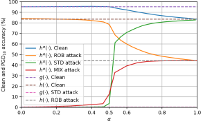
Figure 2: The performance of the mixed classifier $h^{\alpha}(\cdot)$. “STD attack”, “ROB attack”, and “MIX attack” refer to the PGD₂₀ attack generated using the gradient of $g(\cdot)$, $h(\cdot)$, and $h^{\alpha}(\cdot)$ respectively, with $\epsilon$ set to $\frac{8}{255}$.

When $\alpha$ is around $0.5$, the MIX-attacked accuracy of $h^{\alpha}(\cdot)$ quickly increases from near zero to more than $30\%$ (which is two third of $h(\cdot)$’s attacked accuracy). This observation precisely matches the theoretical intuition provided by Theorem 1. On the other hand, when $\alpha$ is greater than $0.5$, the clean accuracy gradually decreases at a much slower rate, leading to the noticeably alleviated accuracy-robustness trade-off.

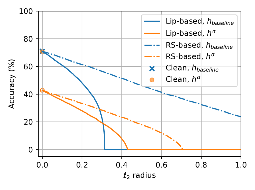
(a) $h_{\text{baseline}}(\cdot)$: RS with $\sigma=0.5$.               
         $h^{\alpha}(\cdot)$: $\alpha=0.76$ and $h(\cdot)$ is RS with $\sigma=1$.

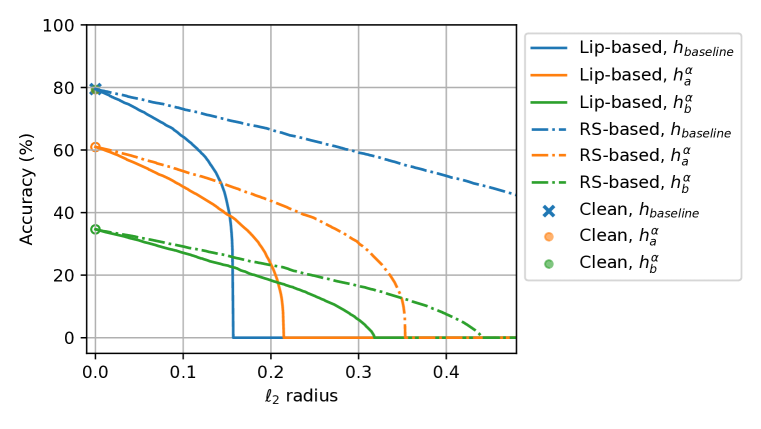
(b) $h_{\text{baseline}}(\cdot)$: RS with $\sigma=0.25$.                                    
Consider two mixed classifier examples:                  
$h^{\alpha}_{a}(\cdot)$: $\alpha=0.76$ and $h_{a}(\cdot)$ is RS with $\sigma=0.5$;         
$\hskip 0.56905pth^{\alpha}_{b}(\cdot)$: $\alpha=0.67$ and $h_{b}(\cdot)$ is RS with $\sigma=1.0$.         

Figure 3: Comparing the certified accuracy-robustness trade-off of RS models and our mixed classifier using both Lipschitz-based (Lip-based) certificates and RS-based certificates (Theorems 1 and 2, respectively). The clean accuracies are the same between $h_{\text{baseline}}(\cdot)$ and $h^{\alpha}(\cdot)$ in each subfigure, and the empty circles represent discontinuity in the certified accuracy at radius $0$.

This difference in how clean and attacked accuracies change with $\alpha$ can be explained by the prediction confidence of $h(\cdot)$. Specifically, according to Table I, $h(\cdot)$ can make correct predictions under attack relatively confidently (average robustness margin is 0.767). Thus, once $\alpha$ becomes greater than $0.5$ and gives $h(\cdot)$ more authority over $g(\cdot)$, $h(\cdot)$ can use this confidence to correct $g(\cdot)$’s mistakes. On the other hand, $h(\cdot)$ is unconfident when it produces incorrect predictions on clean data (the gap between the top two classes is only 0.434). In contrast, $g(\cdot)$ is highly accurate and confident on clean data, but also makes confident mistakes when under attack. As a result, even when $\alpha\geq 0.5$ and $g(\cdot)$ is less powerful than $h(\cdot)$, $g(\cdot)$ can still correct some of the mistakes from $h(\cdot)$ on clean data. In other words, $h(\cdot)$’s confidence difference between correctly predicted attacked examples and incorrectly predicted clean ones is the key source of the improved accuracy-robustness trade-off.

Table I: Average gap between the probabilities of the predicted class and the runner-up class.

	Clean data		PGD20 data
	Correct	Incorrect	Correct	Incorrect
$g(\cdot)$	0.982	0.698	0.559	0.998
$h(\cdot)$	0.854	0.434	0.767	0.636

IV-B Visualization of the Certified Robust Radii

Next, we visualize the certified robust radii presented in Theorem 1 and Theorem 2. Since a (Gaussian) RS model with smoothing covariance matrix $\sigma^{2}I_{d}$ has an $\ell_{2}$-Lipschitz constant $\sqrt{\frac{2}{\pi\sigma^{2}}}$, such a model can be used to simultaneously visualize both theorems, with Theorem 2 giving tighter certificates of robustness. Note that RS models with a larger smoothing variance certify larger radii but achieve lower clean accuracies, and vice versa. Here, we consider the CIFAR-10 dataset and select $g(\cdot)$ to be a ConvNeXT-T model with a clean accuracy of $97.25\%$, and use the RS models presented in [25] as $h(\cdot)$. For a fair comparison, we select an $\alpha$ value such that the clean accuracy of the constructed mixed classifier $h^{\alpha}(\cdot)$ matches that of another RS model $h_{\text{baseline}}(\cdot)$ with a smaller smoothing variance. The expectation term in the RS formulation is approximated with the empirical mean of $10000$ random perturbations drawn from ${\mathcal{N}}(0,\sigma^{2}I_{d})$, and the certified radii of $h_{\text{baseline}}(\cdot)$ are calculated using Theorems 1 and 2 by setting $\alpha$ to $1$. Fig. 3 displays the calculated certified accuracies of $h^{\alpha}(\cdot)$ and $h_{\text{baseline}}(\cdot)$ at various attack radii. The ordinate “Accuracy” at a given abscissa “$\ell_{2}$ radius” reflects the percentage of the test data for which the considered model gives a correct prediction as well as a certified radius at least as large as the $\ell_{2}$ radius under consideration.

In both subplots of Fig. 3, the certified robustness curves of $h^{\alpha}(\cdot)$ do not connect to the clean accuracy when $\alpha$ approaches zero. This is because Theorems 1 and 2 both consider robustness with respect to $h(\cdot)$ and do not issue certificates to test inputs at which $h(\cdot)$ makes incorrect predictions, even if $h^{\alpha}(\cdot)$ predicts correctly at some of these points. This is reasonable because we do not assume any robustness or Lipschitzness of $g(\cdot)$, and $g(\cdot)$ is allowed to be arbitrarily incorrect whenever the radius is non-zero.

Table II: Experiment settings for comparing the choices of $R_{i}(x)$.

	Attack Budget and PGD Steps	$g(\cdot)$ Architecture	$h(\cdot)$ Architecture
Fig. 1	$\ell_{\infty}$, $\epsilon=\frac{8}{255}$, 10 Steps	Standard ResNet18	$\ell_{\infty}$-adversarially-trained ResNet18
Fig. 4(a)	$\ell_{\infty}$, $\epsilon=\frac{8}{255}$, 20 Steps	Standard ConvNeXT-T	TRADES WideResNet-34
Fig. 4(b)	$\ell_{2}$, $\epsilon=0.5$, 20 Steps	Standard ResNet18	$\ell_{2}$-adversarially-trained ResNet18

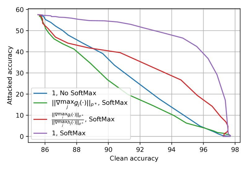
(a) ConvNeXT-T and TRADES WRN-34 under $\ell_{\infty}$ PGD attack.

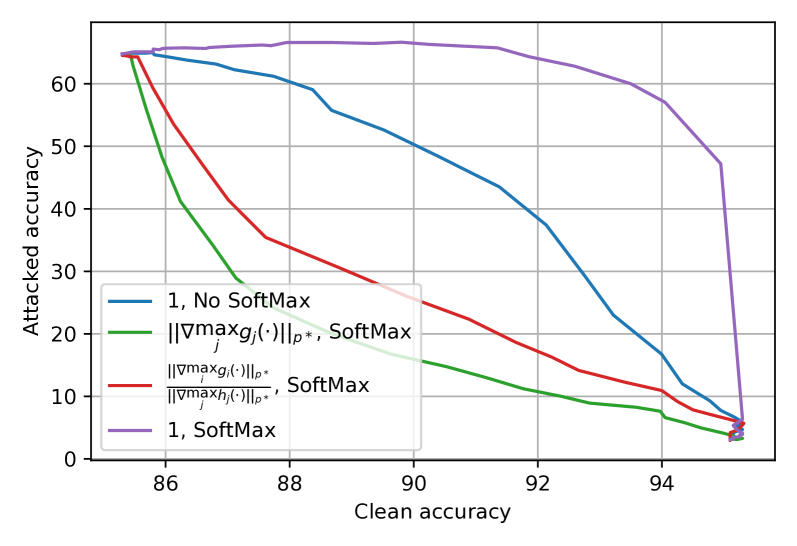
(b) Standard and AT ResNet18s under $\ell_{2}$ PGD attack.

Figure 4: Comparing the options for $R_{i}(x)$ with alternative selections of base classifiers.

The Lipschitz-based bound of Theorem 1 allows us to visualize the performance of the mixed classifier $h^{\alpha}(\cdot)$ when $h(\cdot)$ is an $\ell_{2}$-Lipschitz model. In this case, the curves associated with $h^{\alpha}(\cdot)$ and $h_{\text{baseline}}(\cdot)$ intersect, with $h^{\alpha}(\cdot)$ achieving higher certified accuracy at larger radii and $h_{\text{baseline}}(\cdot)$ certifying more points at smaller radii. By adjusting $\alpha$ and the Lipschitz constant of $h(\cdot)$, it is possible to change the location of this intersection while maintaining the same level of clean accuracy. Therefore, the mixed classifier structure allows for optimizing the certified accuracy at a particular radius, while keeping the clean accuracy unchanged.

The RS-based bound from Theorem 2 captures the behavior of $h^{\alpha}(\cdot)$ when $h(\cdot)$ is an RS model. For both $h^{\alpha}(\cdot)$ and $h_{\text{baseline}}(\cdot)$, the RS-based bounds certify larger radii than the corresponding Lipschitz-based bounds. Nonetheless, $h_{\text{baseline}}(\cdot)$ can certify more points with the RS-based guarantee. Intuitively, this phenomenon suggests that RS models can yield correct but low-confidence predictions when under attack with a large radius, and thus may not be best-suited for our mixing operation, which relies on robustness with non-zero margins. In contrast, Lipschitz models, a more general and common class of models, exploit the mixing operation more effectively. Moreover, as shown in Fig. 2, empirically robust models often yield high-confidence predictions when under attack, making them more suitable to be used as the robust base classifier for $h^{\alpha}(\cdot)$.

IV-C Additional Empirical Support for $R_{i}(x)=1$

Finally, we use additional empirical evidence (Figures 4(a) and 4(b)) to show that $R_{i}(x)=1$ is the appropriate choice for the mixed classifier and that the probabilities should be used for the mixture. While most experiments in this paper are based on the popular ResNet architecture, our method does not depend on any ResNet properties. Therefore, for the experiment in Fig. 4(a), we select a more modern ConvNeXT-T model [57] pre-trained on ImageNet-1k as an alternative architecture for $g(\cdot)$. We also use a robust model trained via TRADES in place of an adversarially-trained network for $h(\cdot)$ for the interest of diversity. Additionally, although most of our experiments are based on $\ell_{\infty}$ attacks, the proposed method applies to all $\ell_{p}$ attack budgets. In Fig. 4(b), we provide an example that considers the $\ell_{2}$ attack. The experiment settings are summarized in Table II.

Figures 4(a) and 4(b) confirm that setting $R_{i}(x)$ to the constant $1$ achieves the best trade-off curve between clean and attacked accuracy, and that mixing the probabilities outperforms mixing the logits. This result aligns with the conclusions of Fig. 1 and our theoretical analyses.

For all three cases listed in Table II, the mixed classifier reduces the error rate of $h(\cdot)$ on clean data by half while maintaining $80\%$ of $h(\cdot)$’s attacked accuracy. This observation suggests that the mixed classifier noticeably alleviates the accuracy-robustness trade-off. Additionally, our method is especially suitable for applications where the clean accuracy gap between $g(\cdot)$ and $h(\cdot)$ is large. On easier datasets such as MNIST and CIFAR-10, this gap has been greatly reduced by the latest advancements in constructing robust classifiers. However, on harder tasks such as CIFAR-100 and ImageNet-1k, this gap is still large, even for state-of-the-art methods. For these applications, standard classifiers often benefit much more from pre-training on larger datasets than robust models.

V Conclusions

This paper proposes a mixed classifier that leverages the mixture of an accurate classifier and a robust classifier to mitigate the accuracy-robustness trade-off of deep models. Since the two base classifiers can be pre-trained, the mixed classifier requires no additional training. Empirical results show that our method can approach the high accuracy of the latest standard models while retaining the robustness achieved by state-of-the-art robust classification methods. Moreover, we mathematically prove that the mixed classifier inherits the certified robustness of the robust base model under realistic assumptions. By varying the Lipschitz constant of the robust base classifier, the mixed classifier allows for optimizing the certified robustness at a particular radius without sacrificing clean accuracy. Consequently, this work provides a foundation for future research to focus on either accuracy or robustness without sacrificing the other, providing additional incentives for deploying robust models in safety-critical control.

References

- [1] S. Levine, C. Finn, T. Darrell, and P. Abbeel, “End-to-end training of deep visuomotor policies,” The Journal of Machine Learning Research, vol. 17, no. 1, pp. 1334–1373, 2016.
- [2] R. S. Sutton and A. G. Barto, Reinforcement Learning: An Introduction. MIT press, 2018.
- [3] M. Bojarski, D. Del Testa, D. Dworakowski, B. Firner, B. Flepp, P. Goyal, L. D. Jackel, M. Monfort, U. Muller, J. Zhang, et al., “End to end learning for self-driving cars,” arXiv preprint arXiv:1604.07316, 2016.
- [4] B. Wu, F. Iandola, P. H. Jin, and K. Keutzer, “SqueezeDet: Unified, small, low power fully convolutional neural networks for real-time object detection for autonomous driving,” in IEEE Conference on Computer Vision and Pattern Recognition Workshops, 2017.
- [5] C. Szegedy, W. Zaremba, I. Sutskever, J. Bruna, D. Erhan, I. Goodfellow, and R. Fergus, “Intriguing properties of neural networks,” in International Conference on Learning Representations, 2014.
- [6] A. Nguyen, J. Yosinski, and J. Clune, “Deep neural networks are easily fooled: High confidence predictions for unrecognizable images,” in IEEE Conference on Computer Vision and Pattern Recognition, 2015.
- [7] S. H. Huang, N. Papernot, I. J. Goodfellow, Y. Duan, and P. Abbeel, “Adversarial attacks on neural network policies,” in International Conference on Learning Representations, 2017.
- [8] K. Eykholt, I. Evtimov, E. Fernandes, B. Li, A. Rahmati, C. Xiao, A. Prakash, T. Kohno, and D. Song, “Robust physical-world attacks on deep learning visual classification,” in IEEE Conference on Computer Vision and Pattern Recognition, 2018.
- [9] A. Liu, X. Liu, J. Fan, Y. Ma, A. Zhang, H. Xie, and D. Tao, “Perceptual-sensitive GAN for generating adversarial patches,” in The AAAI Conference on Artificial Intelligence, 2019.
- [10] A. Kurakin, I. J. Goodfellow, and S. Bengio, “Adversarial machine learning at scale,” in International Conference on Learning Representations, 2017.
- [11] I. J. Goodfellow, J. Shlens, and C. Szegedy, “Explaining and harnessing adversarial examples,” in International Conference on Learning Representations, 2015.
- [12] Y. Bai, T. Gautam, Y. Gai, and S. Sojoudi, “Practical convex formulation of robust one-hidden-layer neural network training,” American Control Conference, 2022.
- [13] Y. Bai, T. Gautam, and S. Sojoudi, “Efficient global optimization of two-layer ReLU networks: Quadratic-time algorithms and adversarial training,” SIAM Journal on Mathematics of Data Science, 2022.
- [14] H. Zheng, Z. Zhang, J. Gu, H. Lee, and A. Prakash, “Efficient adversarial training with transferable adversarial examples,” in IEEE Conference on Computer Vision and Pattern Recognition, 2020.
- [15] B. Anderson, Z. Ma, J. Li, and S. Sojoudi, “Tightened convex relaxations for neural network robustness certification,” in IEEE Conference on Decision and Control, 2020.
- [16] Z. Ma and S. Sojoudi, “A sequential framework towards an exact SDP verification of neural networks,” in International Conference on Data Science and Advanced Analytics, 2021.
- [17] B. G. Anderson and S. Sojoudi, “Data-driven certification of neural networks with random input noise,” IEEE Transactions on Control of Network Systems, 2022.
- [18] J. Cohen, E. Rosenfeld, and Z. Kolter, “Certified adversarial robustness via randomized smoothing,” in International Conference on Machine Learning, 2019.
- [19] B. Li, C. Chen, W. Wang, and L. Carin, “Certified adversarial robustness with additive noise,” in Advances in Neural Information Processing Systems, 2019.
- [20] S. Pfrommer, B. G. Anderson, and S. Sojoudi, “Projected randomized smoothing for certified adversarial robustness,” Transactions on Machine Learning Research, 2023.
- [21] A. Kumar, A. Levine, and S. Feizi, “Policy smoothing for provably robust reinforcement learning,” in International Conference on Learning Representations, 2022.
- [22] F. Wu, L. Li, Z. Huang, Y. Vorobeychik, D. Zhao, and B. Li, “CROP: Certifying robust policies for reinforcement learning through functional smoothing,” in International Conference on Learning Representations, 2022.
- [23] B. G. Anderson and S. Sojoudi, “Certified robustness via locally biased randomized smoothing,” in Learning for Dynamics and Control Conference, 2022.
- [24] D. Tsipras, S. Santurkar, L. Engstrom, A. Turner, and A. Madry, “Robustness may be at odds with accuracy,” in International Conference on Learning Representations, 2019.
- [25] H. Zhang, Y. Yu, J. Jiao, E. P. Xing, L. E. Ghaoui, and M. I. Jordan, “Theoretically principled trade-off between robustness and accuracy,” in International Conference on Machine Learning, 2019.
- [26] Y. Yang, C. Rashtchian, H. Zhang, R. R. Salakhutdinov, and K. Chaudhuri, “A closer look at accuracy vs. robustness,” in Annual Conference on Neural Information Processing Systems, 2020.
- [27] A. Lamb, V. Verma, J. Kannala, and Y. Bengio, “Interpolated adversarial training: Achieving robust neural networks without sacrificing too much accuracy,” in ACM Workshop on Artificial Intelligence and Security, 2019.
- [28] A. Raghunathan, S. M. Xie, F. Yang, J. C. Duchi, and P. Liang, “Understanding and mitigating the tradeoff between robustness and accuracy,” in International Conference on Machine Learning, 2020.
- [29] H. Zhang and J. Wang, “Defense against adversarial attacks using feature scattering-based adversarial training,” in Annual Conference on Neural Information Processing Systems, 2019.
- [30] F. Tramèr, A. Kurakin, N. Papernot, I. J. Goodfellow, D. Boneh, and P. D. McDaniel, “Ensemble adversarial training: Attacks and defenses,” in International Conference on Learning Representations, 2018.
- [31] Y. Balaji, T. Goldstein, and J. Hoffman, “Instance adaptive adversarial training: Improved accuracy tradeoffs in neural nets,” arXiv preprint arXiv:1910.08051, 2019.
- [32] T. Chen, S. Liu, S. Chang, Y. Cheng, L. Amini, and Z. Wang, “Adversarial robustness: From self-supervised pre-training to fine-tuning,” in IEEE Conference on Computer Vision and Pattern Recognition, 2020.
- [33] L. Fan, S. Liu, P.-Y. Chen, G. Zhang, and C. Gan, “When does contrastive learning preserve adversarial robustness from pretraining to finetuning?” in Advances in Neural Information Processing Systems, 2021.
- [34] A. Madry, A. Makelov, L. Schmidt, D. Tsipras, and A. Vladu, “Towards deep learning models resistant to adversarial attacks,” in International Conference on Learning Representations, 2018.
- [35] N. Carlini and D. A. Wagner, “Towards evaluating the robustness of neural networks,” in IEEE Symposium on Security and Privacy, 2017.
- [36] A. Athalye, N. Carlini, and D. Wagner, “Obfuscated gradients give a false sense of security: Circumventing defenses to adversarial examples,” in International Conference on Machine Learning, 2018.
- [37] N. Papernot, P. McDaniel, I. Goodfellow, S. Jha, Z. B. Celik, and A. Swami, “Practical black-box attacks against machine learning,” in ACM Asia Conference on Computer and Communications Security, 2017.
- [38] F. Croce and M. Hein, “Reliable evaluation of adversarial robustness with an ensemble of diverse parameter-free attacks,” in International Conference on Machine Learning, 2020.
- [39] F. Tramèr, N. Carlini, W. Brendel, and A. Madry, “On adaptive attacks to adversarial example defenses,” in Advances in Neural Information Processing Systems, 2020.
- [40] L. Schmidt, S. Santurkar, D. Tsipras, K. Talwar, and A. Madry, “Adversarially robust generalization requires more data,” Advances in Neural Information Processing Systems, vol. 31, 2018.
- [41] S.-A. Rebuffi, S. Gowal, D. A. Calian, F. Stimberg, O. Wiles, and T. Mann, “Fixing data augmentation to improve adversarial robustness,” arXiv preprint arXiv:2103.01946, 2021.
- [42] S. Gowal, S.-A. Rebuffi, O. Wiles, F. Stimberg, D. A. Calian, and T. Mann, “Improving robustness using generated data,” arXiv preprint arXiv:2110.09468, 2021.
- [43] V. Sehwag, S. Mahloujifar, T. Handina, S. Dai, C. Xiang, M. Chiang, and P. Mittal, “Robust learning meets generative models: Can proxy distributions improve adversarial robustness?” in International Conference on Learning Representations, 2022.
- [44] X. Jia, Y. Zhang, B. Wu, K. Ma, J. Wang, and X. Cao, “LAS-AT: Adversarial training with learnable attack strategy,” in IEEE Conference on Computer Vision and Pattern Recognition, 2022.
- [45] A. Shafahi, M. Najibi, M. A. Ghiasi, Z. Xu, J. Dickerson, C. Studer, L. S. Davis, G. Taylor, and T. Goldstein, “Adversarial training for free!” Advances in Neural Information Processing Systems, 2019.
- [46] T. Pang, M. Lin, X. Yang, J. Zhu, and S. Yan, “Robustness and accuracy could be reconcilable by (proper) definition,” arXiv preprint arXiv:2202.10103, 2022.
- [47] T. Hu, T. Chen, H. Wang, and Z. Wang, “Triple wins: Boosting accuracy, robustness and efficiency together by enabling input-adaptive inference,” in International Conference on Learning Representations, 2020.
- [48] Y. Zheng, R. Zhang, and Y. Mao, “Regularizing neural networks via adversarial model perturbation,” in IEEE Conference on Computer Vision and Pattern Recognition, 2021.
- [49] X. Liu, M. Cheng, H. Zhang, and C.-J. Hsieh, “Towards robust neural networks via random self-ensemble,” in European Conference on Computer Vision, 2018.
- [50] T. Pang, K. Xu, C. Du, N. Chen, and J. Zhu, “Improving adversarial robustness via promoting ensemble diversity,” in International Conference on Machine Learning, 2019.
- [51] M. Alam, S. Datta, D. Mukhopadhyay, A. Mondal, and P. P. Chakrabarti, “Resisting adversarial attacks in deep neural networks using diverse decision boundaries,” arXiv preprint arXiv:2208.08697, 2022.
- [52] A. Krizhevsky, “Learning multiple layers of features from tiny images,” 2012. [Online]. Available: https://www.cs.toronto.edu/~kriz/learning-features-2009-TR.pdf
- [53] H. Salman, J. Li, I. Razenshteyn, P. Zhang, H. Zhang, S. Bubeck, and G. Yang, “Provably robust deep learning via adversarially trained smoothed classifiers,” Advances in Neural Information Processing Systems, 2019.
- [54] M. Fazlyab, A. Robey, H. Hassani, M. Morari, and G. Pappas, “Efficient and accurate estimation of Lipschitz constants for deep neural networks,” in Advances in Neural Information Processing Systems, 2019.
- [55] M. Hein and M. Andriushchenko, “Formal guarantees on the robustness of a classifier against adversarial manipulation,” in Advances in Neural Information Processing Systems, 2017.
- [56] A. Levine, S. Singla, and S. Feizi, “Certifiably robust interpretation in deep learning,” arXiv preprint arXiv:1905.12105, 2019.
- [57] Z. Liu, H. Mao, C.-Y. Wu, C. Feichtenhofer, T. Darrell, and S. Xie, “A ConvNet for the 2020s,” in IEEE Conference on Computer Vision and Pattern Recognition, 2022.