Hessian Aware Low-Rank Weight Perturbation for Continual Learning

Abstract

Continual learning aims to learn a series of tasks sequentially without forgetting the knowledge acquired from the previous ones. In this work, we propose the Hessian Aware Low-Rank Perturbation algorithm for continual learning. By modeling the parameter transitions along the sequential tasks with the weight matrix transformation, we propose to apply the low-rank approximation on the task-adaptive parameters in each layer of the neural networks. Specifically, we theoretically demonstrate the quantitative relationship between the Hessian and the proposed low-rank approximation. The approximation ranks are then globally determined according to the marginal increment of the empirical loss estimated by the layer-specific gradient and low-rank approximation error. Furthermore, we control the model capacity by pruning less important parameters to diminish the parameter growth. We conduct extensive experiments on various benchmarks, including a dataset with large-scale tasks, and compare our method against some recent state-of-the-art methods to demonstrate the effectiveness and scalability of our proposed method. Empirical results show that our method performs better on different benchmarks, especially in achieving task order robustness and handling the forgetting issue. The source code can be found at https://github.com/lijiaqi/HALRP.

1 Introduction

The conventional machine learning paradigm assumes all the data are simultaneously accessed and trained. However, in practical scenarios, data are often collected from different tasks and sequentially accessed in a specific order. Continual Learning (CL) aims to gradually learn from novel tasks and preserve valuable knowledge from previous ones. Despite this promising paradigm, CL is usually faced with a dilemma between memory stability and learning plasticity: when adapting among the dynamic data distributions, it has been shown that the neural networks can easily forget the learned knowledge of previous tasks when facing a new one, which is known as Catastrophic Forgetting (CF) [1].

One possible reason for this forgetting issue can be the parameter drift from the previous tasks to the new ones, which is caused by the optimization process with the use of stochastic gradient descent and its variants [2, 3]. To mitigate the obliviousness to past knowledge, some works [4, 5, 6, 7, 8] proposed to constrain the optimization objective for the knowledge of new tasks with additional penalty regularization terms. These approaches were shown as ineffective under the scenarios of a large number of tasks, lacking long-term memory stability in real-world applications.

To address this problem, some methods choose to expand the model during the dynamic learning process in a specific way, leading to inferencing with task-specific parameters for each task. For example, a recent work [9] proposed to decompose the model as task-private and task-shared parameters via an additive model parameters decomposition. However, this method only applies an attention vector for the masking of the task-shared parameters. Furthermore, the private parameters were controlled by a regularization and consolidation process, which lead to the linear model increment along with the increasing task number, damaging the scalability for deploying a CL system. Another solution to reduce the parameter increase is applying factorization for the model parameters. In this regard, [10] proposed a low-rank factorization method for the model parameters decomposition with a Bayesian process inference. However, this approach required a large rank for achieving desirable accuracy and also suffered from ineffectiveness in some complex data scenarios.

In this work, we propose a low-rank perturbation method to learn the relationship between the learned model (base parameters) and the parameters for new tasks. By formulating a flexible weight transition process, the model parameters during the CL scenario are decomposed as task-shared ones and task-adaptive ones. The former can be adopted from the base task to new tasks. The latter conforms to a low-rank matrix, and the number of relevant parameters can be effectively reduced for every single layer in a neural network across the tasks. With a simple warm-up training strategy, the low-rank task-adaptive parameters can be efficiently initialized with singular value decomposition.

Furthermore, to determine which ranks should be preserved for the low-rank approximation in different layers in a model, we propose to measure the influences of the introduced low-rank parameters by the Hessian-aware risk perturbation across layers of the whole model. This allows the model to automatically assign larger ranks to a layer that contributes more to the final performance under a specific parameter size budget. We theoretically support this approach by providing a formal demonstration that the empirical losses derived from the proposed low-rank perturbation are bounded by the Hessian and the approximation rate of the decomposition. This leads to a Hessian-aware framework that enables the model to determine perturbation ranks that minimize the overall empirical error. Lastly, we apply a pruning technique to control the introduced parameter size and reduce some less important perturbation parameters through the aforementioned Hessian-aware framework by evaluating their importance.

Based on the theoretical analysis, we proposed the Hessian Aware Low-Rank Perturbation (HALRP) algorithm, which enables the model to leverage the Hessian information to automatically apply the low-rank perturbation according to a certain approximation rate. To summarize, the contributions of our work mainly lie in three-fold:

• We proposed a Hessian aware low-rank perturbations framework that allows efficient memory and computation requests for learning continual tasks.

• Theoretical analyses were investigated to show that Hessian information can be used to quantitatively measure the influences of low-rank perturbation on the empirical risk. This leads to an automatic rank selection process to control the model increment.

• Extensive experiments on several benchmarks and recent state-of-the-art baselines (e.g., regularization-, expansion-, and memory-based) were conducted to demonstrate the effectiveness of our method. The results testify the superiority of our HALRP, in terms of accuracy, computational efficiency, scalability, and task-order robustness.

2 Related Work

Regularization-based approaches diminish catastrophic forgetting by penalizing the parameter drift from the previous tasks using different regularizers [4, 5, 6]. Batch Ensemble [11] designed an ensemble weight generation method by the Hadamard product between a shared weight among all ensemble members and an ensemble member-specific rank-one matrix. In [12], the regularizer on the adaptive group sparsity was used to guarantee the exact sparsity and freezing of the model. [13] indicated that learning tasks in different low-rank vector subspaces orthogonal to each other can minimize task interferences. Functional regularizer [6], a Bayesian inference framework over the function space, tried to construct and memorize an approximate posterior belief over the underlying task-specific function. [14] applied a regularizer with decoupled prototype-based loss, which can improve the intra-class and inter-class structure significantly. Compared to this kind of approach, our method applied task-specific parameters and introduced an explicit weight transition process to leverage the knowledge from the previous tasks and overcome the forgetting issue.

Expansion-based methods utilize different subsets of model parameters for each task. [15] proposed to memorize the learned knowledge by freezing the base model and progressively expanding the new sub-model for new tasks. In [16], the reuse and expansion of networks were achieved dynamically by selective retraining, with splitting or duplicating components for newly coming tasks. Some work (e.g., [17]) tried to determine the optimal network growth by neural architecture search. To balance memory stability and learning plasticity, [18] adopted a distillation-based method under the class incremental scenario. To achieve the scalability and the robustness of task orders, Additive Parameter Decomposition (APD) [9] adopted sparse task-specific parameters for novel tasks in addition to the dense task-shared ones and performed hierarchical consolidation within similar task groups for the further knowledge sharing. More recently, Winning Subnetworks (WSN) [19] jointly learned shared network weights and binary masks for each task to avoid retraining. To address the forgetting issue, only the model weights that had not been selected in the previous tasks were tendentiously updated during training. However, this method still needs to store task-specific mask information for the inference stage and relies on extra compression processes for mask encoding to achieve scalability.

Replay (memory) based approaches usually leverage different types of replay buffers (e.g., [20, 21, 13, 22, 23, 24, 25]) to memorize a small episode of the previous tasks, which can be rehearsed when learning the novel ones to avoid forgetting. In [25], a dynamic prototype-guided memory replay module was incorporated with an online meta-learning framework to reduce memory occupation. [26] proposed to process both specific and generalized information by the interplay of three memory networks. To avoid the repeated inferences on previous tasks, Gradient Episodic Memory [2] and its variant [27] projected the new gradients into a feasible region that is determined by the gradients on previous task samples. Instead, Gradient Projection Memory (GPM) [2] chose to directly store the bases of previous gradient spaces to guide the direction of parameters update on new tasks. Compared to these approaches, our proposed method does not rely on extra storage for the data or gradient information of previous tasks, avoiding privacy leakage under some sensitive scenarios.

Low-rank Factorization for CL Low-rank factorization [28] has been widely studied in deep learning to decompose the parameters for model compression [29, 30] or data projection [31, 32]. In the context of CL, [10] considers the low-rank model factorization and automatic rank selection per task for variational inference, which requires significantly large rank increments per task to achieve high accuracy. GPM  [2] applied the singular value decomposition on the representations and store them in the memory. [13] proposed to learn tasks by low-rank vector sub-spaces to avoid a joint vector space that may lead to interferences among tasks. The most similar work is Incremental Rank Updates (IRU) [33]. Compared to the decomposition in IRU, we adopted the low-rank approximation on the residual representation in the weights transitions. Furthermore, the rank selection in our work was dynamically and automatically determined according to Hessian-aware perturbations, rather than the manual rank increment in [33].

TABLE I: List of main notations.

Notation	Description
$T$,$t$	Total task number, task index
$\mathcal{T}_{t},\mathcal{D}_{t}$	$t$-th task, and the related dataset
$\mathbf{x},y$	input/sample, class label
$\mathbf{W}$	model weights
$\mathbf{R},\mathbf{S},\mathbf{B}$	task private model weights
$\mathbf{U},\boldsymbol{\Sigma},\mathbf{V}$	SVD decomposition on $\mathbf{B}$ shown in Sect. 3.2
$\mathrm{diag}(\boldsymbol{\Sigma})$	diagonal elements of $\boldsymbol{\Sigma}$
$\mathrm{Diag}(\sigma_{1},\cdots,\sigma_{n})$	diagonal matrix with elements $\{\sigma_{1},\cdots,\sigma_{n}\}$
$\mathbf{M}^{(k)}$	$k$-rank low-rank approximation of $\mathbf{M}$
$\|\cdot\|_{F}$	Frobenius norm
$\mathcal{L}$	loss function for the task (e.g, cross-entropy)
$\mathcal{L}_{\text{reg}}$	regularization loss
$\mathbf{H}$	Hessian matrix
$\alpha$	loss approximation rate for rank selection
$l$	layer index in a neural network
$\mathbf{g}_{l}$	gradient vector for layer $l$
$r_{l}$	full rank of layer $l$
$k_{l}$	approximated rank for layer $l$
$n$	number of total training epochs
$n_{r}$	number of warm-up epochs

3 Preliminary and Background

This section introduces the basic knowledge of continual learning and singular value decomposition [34]. In Table I, we provide a list of the main notations used in our paper. Specifically, the bold uppercase (or lowercase) letters indicate the matrices (or vectors) in the remaining part.

3.1 Continual Learning

Assume the learner receives a series of $T$ tasks $\{\mathcal{T}_{0},\dots,\mathcal{T}_{T-1}\}$ sequentially, and denote the dataset of the $t^{th}$ task as $\mathcal{D}_{t}=\{\mathbf{x}^{i}_{t},y^{i}_{t}\}_{i=1}^{N_{t}}$, where $\mathbf{x}^{i}_{t}$ and $y^{i}_{t}$ corresponds to the $i^{th}$ instance and label in the total of $N_{t}$ data points. In the context of CL, the dataset $\mathcal{D}_{t}$ will become inaccessible after the time step $t$.

3.2 Low-Rank Approximation of Matrix with SVD

The singular value decomposition (SVD) factorizes a rectangular matrix $\mathbf{B}\in\mathbb{R}^{J\times I}$ with three matrices: $\mathbf{B}=\mathbf{U}\boldsymbol{\Sigma}\mathbf{V}^{\top}$, where $\mathbf{U}\in\mathbb{R}^{J\times J}$, $\mathbf{V}\in\mathbb{R}^{I\times I}$, and $\boldsymbol{\Sigma}\in\mathbb{R}^{J\times I}$. Denote the rank of $\mathbf{B}$ with $r\leq\min\{I,J\}$, then $\mathbf{B}$ can be further expressed as $\mathbf{B}=\sum_{i=1}^{r}\sigma_{i}\mathbf{u}_{i}\mathbf{v}_{i}^{\top}$, where $\sigma_{i}\in\mathrm{diag}(\boldsymbol{\Sigma})$ is the singular values, $\mathbf{u}_{i}$ and $\mathbf{v}_{i}$ are respectively the left and right singular vectors. In this work, we take the property of $k$-rank approximation of $\mathbf{B}$ (with $k\leq r$) by leveraging the Eckart–Young–Mirsky theorem [35], which can be expressed with top-$k$ leading singular values and vectors: $\mathbf{B}^{(k)}=\mathbf{U}^{(k)}\boldsymbol{\Sigma}^{(k)}\mathbf{V}^{(k)\top}=\sum_{i=1}^{k}\sigma_{i}\mathbf{u}_{i}\mathbf{v}_{i}^{\top}$, where $\mathbf{U}^{(k)}$, $\boldsymbol{\Sigma}^{(k)}$, $\mathbf{V}^{(k)}$ are the corresponding leading principal sub-matrices. $k$ is chosen to tolerate a certain approximation error under the Frobenius norm $\|\cdot\|_{F}$ (See Appendix A for the proof):

$$\begin{split}\|\mathbf{B}-\mathbf{B}^{(k)}\|_{F}=\sqrt{\sigma_{k+1}^{2}+\dots+\sigma_{r}^{2}}\end{split}$$ (1)

4 Methodology

Our framework leverages the low-rank approximation of neural network weights. In the following parts, we present the methodology for handling the fully connected layers and the convolutional layers. The analysis herein can be applied to any layer of the model. Without loss of generality, we omit the layer index $l$ in this section. For simplicity, we illustrate the learning process using tasks $\mathcal{T}_{0}$ and $\mathcal{T}_{1}$ in Sections 4.1 and 4.2, which can be applied to the successive new tasks as shown in Section 4.5.

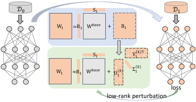
Figure 1: Low rank decomposition between $\mathcal{T}_{1}$ and $\mathcal{T}_{0}$

4.1 Fully Connected Layers

We first consider linear layers of neural networks in a supervised training context. We begin by learning task $\mathcal{T}_{0}$ without any constraints on the model parameters. Specifically, we train the model by minimizing the empirical risk to get the base weights $\mathbf{W}^{\text{base}}=\operatorname*{arg\,min}_{\mathbf{W}}\mathcal{L}(\mathbf{W};\mathcal{D}_{0})$, where $\mathbf{W}^{\text{base}}\in\mathbb{R}^{J\times I}$, $J$ is the output dimension, and $I$ is the input dimension of the layer.

Then, when the task $\mathcal{T}_{1}$ comes to the learner, we can train the model fully on $\mathcal{D}_{1}$ and get the updated weights $\mathbf{W}_{1}\in\mathbb{R}^{J\times I}$. However, undesired model drifts can lead to worse performance on $\mathcal{T}_{0}$ if no constraints are applied to the parameters update. Previous work [4] applied a $L_{2}$ regularization to enforce that the weights learned on the new model will not be too far from those of the previous tasks. Although this kind of method only expands the base model with limited parameters, it can lead to worse performance on both $\mathcal{T}_{0}$ and $\mathcal{T}_{1}$.

To pursue a better trade-off between the model size increment and overall performance on both $\mathcal{T}_{0}$ and $\mathcal{T}_{1}$, we assume the unconstrained trained parameters $\mathbf{W}_{1}$ on $\mathcal{T}_{1}$ can be transformed from $\mathbf{W}^{\text{base}}$ by the low-rank weight perturbation (LRWP, as illustrated in Figure 1),

$$\mathbf{W}_{1}=\mathbf{R}_{1}\mathbf{W}^{\text{base}}\mathbf{S}_{1}+\mathbf{B}_{1}$$ (2)

where $\mathbf{B}_{1}\in\mathbb{R}^{J\times I}$ is a sparse low-rank matrix, $\mathbf{R}_{1}=\textrm{Diag}(r_{1,0},\dots,r_{1,J})$, and $\mathbf{S}_{1}=\textrm{Diag}(s_{1,0},\dots,s_{1,I})$ are task-private parameters for $\mathcal{T}_{1}$.

The form of the proposed low-rank decomposition in Eq. 2 has differences with the additive parameter decomposition proposed in [9]. In fact, the task-adaptive bias term $\mathbf{B}_{1}$ conforms to a low-rank matrix, which reduces both the parameter storage and the computational overhead. Moreover, the task-adaptive mask terms $\mathbf{R}_{1}$ and $\mathbf{S}_{1}$ include both row-wise and column-wise scaling parameters instead of only column-wise parameters like [9] to allow smaller and possibly sparser discrepancy: $\mathbf{B}_{1}=\mathbf{W}_{1}-\mathbf{R}_{1}\mathbf{W}^{\text{base}}\mathbf{S}_{1}.$

In addition, regarding the parameter estimation, we can substitute $\mathbf{B}_{1}$ with its $k$-rank decomposition $\mathbf{B}_{1}^{(k)}=\sum_{i=1}^{k}\sigma_{i}\mathbf{u}_{i}\mathbf{v}_{i}^{\top}$ in Eq. 2 and directly minimize the empirical risk on task $\mathcal{T}_{1}$ to get the parameter estimation through stochastic gradient descent with the random initialization of $\{\mathbf{u}_{i}\}_{i=1}^{k}$ and $\{\mathbf{v}_{i}\}_{i=1}^{k}$. However, in practice, we found it challenging to learn a useful decomposition in this way (i.e., the estimations converge to a local optimum quickly) and the empirical risk minimization does not benefit from the low-rank decomposition. Due to the homogeneity among the one-rank components $\{\mathbf{u}_{i}\mathbf{v}_{i}^{\top}\}_{i=1}^{k}$, random initialization cannot sufficiently distinguish them and hence make the gradient descent ineffective.

To address the aforementioned ineffective training problem, we first train the model fully on task $\mathcal{T}_{1}$ for a few epochs (e.g., one or two) to get rough parameter estimations $\mathbf{W}_{1}^{\text{free}}\in\mathbb{R}^{J\times I}$ of the new task, indicating free-trained weights without any constraints. Then, a good warm-up initialized values for Eq. 2 can then be obtained by solving the following least squared error (LSE) minimization objective,

$$\operatorname*{arg\,min}_{\mathbf{R},\mathbf{S},\mathbf{B}}\|\mathbf{W}_{1}^{\text{free}}-\mathbf{R}\mathbf{W}^{\text{base}}\mathbf{S}-\mathbf{B}\|_{F}^{2}$$ (3)

As $\mathbf{R},\mathbf{S},\mathbf{B}$ can correlate, minimizing them simultaneously can be difficult. Thus, we minimize Eq. 3 alternately. First, fix $\mathbf{S},\mathbf{B}$ and solve $\mathbf{R}$, and so on.

$$\begin{split}&\mathbf{R}_{1}^{\text{free}}=\operatorname*{arg\,min}_{\mathbf{R}}\|\mathbf{W}^{\text{free}}-\mathbf{R}\mathbf{W}^{\text{base}}\|_{F}^{2}\\ &\mathbf{S}_{1}^{\text{free}}=\operatorname*{arg\,min}_{\mathbf{S}}\|\mathbf{W}^{\text{free}}-\mathbf{R}_{1}^{\text{free}}\mathbf{W}^{\text{base}}\mathbf{S}\|_{F}^{2}\\ &\mathbf{B}_{1}^{\text{free}}=\mathbf{W}_{1}^{\text{free}}-\mathbf{R}_{1}^{\text{free}}\mathbf{W}^{\text{base}}\mathbf{S}_{1}^{\text{free}}\end{split}$$ (4)

Eq. 4 can be solved efficiently via LSE minimization. For example, for $\mathbf{R}$, we have $\|\mathbf{W}^{\text{free}}-\mathbf{R}\mathbf{W}^{\text{base}}\|_{F}^{2}=\sum_{i=1}^{I}\sum_{j=1}^{J}(w^{\text{free}}_{ji}-r_{j}w^{\text{base}}_{ji})^{2}$, where $w^{\text{free}}_{ji}$ and $w^{\text{base}}_{ji}$ refer to the elements of $j^{th}$ row and $i^{th}$ column of $\mathbf{W}^{\text{free}}$ and $\mathbf{W}^{\text{base}}$, respectively. Applying derivation w.r.t. $r_{j}$ equals 0, we have $r_{j}=\sum_{i}w_{ji}^{\text{free}}w_{ji}^{\text{base}}/(\sum_{i}w_{ji}^{\text{base}})^{2}$. Then, similarly, we can solve $\mathbf{S}$ and $\mathbf{B}$. Furthermore, with the SVD solver denoted by $\texttt{SVD}(\cdot)$, the values of the low-rank decomposition for $\mathbf{B}^{\text{free}}$ can be obtained

$$\begin{split}\mathbf{U}_{1}^{\text{free}},\boldsymbol{\Sigma}_{1}^{\text{free}},\mathbf{V}_{1}^{\text{free}}&=\texttt{SVD}(\mathbf{B}_{1}^{\text{free}})\end{split}$$ (5)

A $k$-rank decomposition $\mathbf{U}_{1}^{(k){\text{free}}}$, $\boldsymbol{\Sigma}_{1}^{(k){\text{free}}}$, $\mathbf{V}_{1}^{(k){\text{free}}}$ can be obtained by retaining their corresponding leading principal submatrix of order $k\leq r$. So we can obtain a $k$-rank approximation to $\mathbf{W}_{1}^{\text{free}}$ by

$$\mathbf{W}_{1}^{(k){\text{free}}}=\mathbf{R}_{1}^{\text{free}}\mathbf{W}^{\text{base}}\mathbf{S}_{1}^{\text{free}}+\mathbf{B}_{1}^{(k){\text{free}}},$$ (6)

where $\mathbf{B}_{1}^{(k){\text{free}}}=\mathbf{U}^{(k){\text{free}}}\boldsymbol{\Sigma}^{(k){\text{free}}}(\mathbf{V}^{(k){\text{free}}})^{\top}$.

Finally, we can initialize the values in Eq. 2 with $\mathbf{R}_{1}^{\text{free}}$, $\mathbf{S}_{1}^{\text{free}}$, $\mathbf{U}_{1}^{(k){\text{free}}}$, $\boldsymbol{\Sigma}_{1}^{(k){\text{free}}}$ and $\mathbf{V}_{1}^{(k){\text{free}}}$, and then fine-tune their estimates by minimizing the empirical risk on task $\mathcal{T}_{1}$ to achieve better performance. The proposed training technique not only enables well-behaved estimations of the low-rank components but also sheds light on how to select approximation ranks of different layers to achieve an optimal trade-off between model performance and parameter size, as discussed in Section 4.3.

4.2 Convolutional Layers

In addition, we can also decompose the weights of a convolutional layer in a similar way. The size of the convolutional kernel is denoted by $d\times d$. The base weights of the convolution layer for task $\mathcal{T}_{0}$ would be a tensor $\mathbf{W}_{\text{conv}}^{\text{base}}\in\mathbb{R}^{d\times d\times J\times I}$. Similar to Eq. 2, a low-rank weight perturbation for transforming $\mathbf{W}_{\text{conv}}^{\text{base}}$ to $\mathbf{W}_{\text{conv},1}\in\mathbb{R}^{d\times d\times J\times I}$ is,

$$\mathbf{W}_{\text{conv},1}=\mathbf{R}_{\text{conv},1}\otimes\mathbf{W}_{\text{conv}}^{\text{base}}\otimes\mathbf{S}_{\text{conv},1}\oplus\mathbf{B}_{\text{conv},1}$$ (7)

where $\mathbf{R}_{\text{conv},1}\in\mathbb{R}^{1\times 1\times J\times 1}$, $\mathbf{S}_{\text{conv},1}\in\mathbb{R}^{1\times 1\times 1\times I}$ and $\mathbf{B}_{\text{conv},1}\in\mathbb{R}^{1\times 1\times J\times I}$ is sparse low-rank tensor (matrix), $\otimes$ and $\oplus$ are element-wise tensor multiplication and summation operators will automatically expand tensors to be of equal sizes, following the broadcasting semantics of some popular scientific computation package like Numpy [36] or PyTorch [37]. Thus, the number of parameters added through this kind of decomposition is still $\mathcal{O}(I+J)$.

To get the estimations of the introduced parameters, we can solve a similar LSE problem as in Eq. 3 to obtain initial estimates $\mathbf{R}_{\text{conv},1}^{\text{free}}$ and $\mathbf{S}_{\text{conv},1}^{\text{free}}$. Then we take the average of the first two dimensions to transform the discrepancy tensor $(\mathbf{W}_{\text{conv},1}^{\text{free}}-\mathbf{R}_{\text{conv},1}^{\text{free}}\otimes\mathbf{W}_{\text{conv}}^{\text{base}}\otimes\mathbf{S}_{\text{conv},1}^{\text{free}})$ to be a $1\times 1\times J\times I$ tensor, which can then be applied a similar decomposition with the FC layers (Eq. 5 and Eq. 6.) to obtain the low-rank estimates of $\mathbf{B}_{\text{conv},1}^{\text{free}}$.

4.3 Selection of Rank for each layer based on Hessian Information

Sections 4.1 and 4.2 present how the low-rank approximation can be used to transfer knowledge and reduce the number of parameters for a single layer across the tasks in continual learning. However, how to select the preserved rank for each layer remains unsolved. We tackle this problem by measuring how the empirical risk $\mathcal{L}(\mathbf{W})$ is influenced by the introduced low-rank parameters across different layers so that we can assign a larger rank to a layer that contributes more to the risk. Inspired by the previous studies [38, 39] about the relationship between Hessian and quantization errors, we establish the following Theorem 2. The full proof is presented in Appendix B.

Theorem 1.

Assume that a neural network of $L$ layers with vectorized weights $(\boldsymbol{\omega}^{\star}_{1},\dots,\boldsymbol{\omega}^{\star}_{L})$ that have converged to local optima, such that the first and second order optimally conditions are satisfied, i.e., the gradient is zero, and the Hessian is positive semi-definite. Suppose a perturbation $\Delta\boldsymbol{\omega}^{\star}_{1}$ applied to the first layer weights, then we have the loss increment

$$\begin{split}\mathcal{L}(\boldsymbol{\omega}^{\star}_{1}-\Delta\boldsymbol{\omega}^{\star}_{1},&\dots,\boldsymbol{\omega}^{\star}_{L})-\mathcal{L}(\boldsymbol{\omega}^{\star}_{1},\dots,\boldsymbol{\omega}^{\star}_{L})\\ &\leq\|\frac{1}{2}\mathbf{H}_{1}\|_{F}\|\Delta\boldsymbol{\omega}^{\star}_{1}\|^{2}_{F}+o(\|\Delta\boldsymbol{\omega}^{\star}_{1}\|^{2}_{F}),\end{split}$$ (8)

where $\mathbf{H}_{1}=\Delta\mathcal{L}(\boldsymbol{\omega}^{\star}_{1})$ is the Hessian matrix at only the variables of the first layer weights.

In our low-rank perturbation setting, we assume that $\mathbf{W}_{1}^{\text{free}}$ by warm-up training is a local optimum. By Theorem 2, we consider the difference between $\mathbf{W}_{1}^{\text{free}}$ and its $k$-rank approximation $\mathbf{W}_{1}^{(k){\text{free}}}$ as a perturbation $\Delta\mathbf{W}_{1}^{(k){\text{free}}}$ for the weights. Then the amount of perturbation can be computed with the low-rank approximation error:

$$\begin{split}\|\Delta\mathbf{W}_{1}^{(k){\text{free}}}\|_{F}=&\|\mathbf{W}_{1}^{\text{free}}-\mathbf{W}_{1}^{(k){\text{free}}}\|_{F}=\sqrt{\sum_{i=k+1}^{r}\sigma_{i}^{2}}\\ \end{split}$$ (9)

where $\{\sigma_{i}\}_{i=1}^{r}$ are the singular values of $\mathbf{W}_{1}^{\text{free}}$ and $r$ is the matrix rank of $\mathbf{W}_{1}^{\text{free}}$.

Thus, according to Theorem 2, the influence on the loss introduced by this low-rank weight perturbation is given by

$$\begin{split}\mathcal{L}(\mathbf{W}_{1}^{\text{free}}&-\Delta\mathbf{W}_{1}^{(k){\text{free}}})-\mathcal{L}(\mathbf{W}_{1}^{\text{free}})\\ &\leq\|\frac{1}{2}\mathbf{H}_{1}\|_{F}(\sum_{i=1}^{k}\sigma_{i}^{2})+o(\sum_{i=k+1}^{r}\sigma_{i}^{2}).\end{split}$$ (10)

where the Hessian matrix $\mathbf{H}_{1}$ can be approximated by the negative empirical Fisher information [40], i.e., the outer product of the gradient vector for the layer weights. So $\|\mathbf{H}_{1}\|_{F}$ can be approximated by $\|\mathbf{g}_{1}\|_{F}^{2}$, where $\mathbf{g}_{1}=\frac{\partial\mathcal{L}}{\partial W_{1}}\mid_{W_{1}=W_{1}^{\text{free}}}$. Finally, we can quantitatively measure the contribution of the loss of adding a marginal rank $k$ for a particular layer $l$ by $\|\mathbf{g}_{l}\|_{F}^{2}\sigma_{l,k}^{2}$, where $\mathbf{g}_{l}$ is the gradient for the layer-$l$ weights and $\sigma_{l,k}$ is the $k$-th singular value of the free-trained layer-$l$ weights, and sort them by the descending order of importance.

For a given loss approximation rate $\alpha$ (e.g., 0.9), we can determine the rank $k_{l}$ (with $k_{l}\leq r_{l}$ where $r_{l}$ is the total rank of the layer $l$) for each layer $l=0,...,L-1$ by solving

$$\min_{k_{1},...,k_{L-1}}\quad\sum_{l=0}^{L-1}\sum_{i=1}^{k_{l}}\|\mathbf{g}_{l}\|_{F}^{2}\sigma_{l,i}^{2}$$ (11)

$$\text{s.t.}\sum_{l=0}^{L-1}\sum_{i=1}^{k_{l}}\|\mathbf{g}_{l}\|_{F}^{2}\sigma_{l,i}^{2}\geq\alpha\sum_{l=0}^{L-1}\sum_{i=1}^{r_{l}}\|\mathbf{g}_{l}\|_{F}^{2}\sigma_{l,i}^{2}$$

Remark: Eq. 11 enables a dynamic scheme for the trade-off between the approximation precision and computational efficiency. For a given approximation rate, the model can automatically select the rank for all the layers in the model.

4.4 Controlling the Introduced Parameter Sizes

The proposed low-rank perturbation method introduced extra parameters compared to a single-task model. We further control the model growth to improve memory efficiency.

Firstly, by following  [9], we can add regularizations on $\mathbf{U}^{(k){\text{free}}}$, $\mathbf{V}^{(k){\text{free}}}$, $\mathbf{R}^{\text{free}}$,$\mathbf{S}^{\text{free}}$ since second task $\mathcal{T}_{1}$ to enhance the sparsity of the task-private parameters (see Appendix C for more discussion for this fine-tuning objective):

$$\mathcal{L}_{\text{reg}}(\mathbf{W}_{t};\mathcal{D}_{t})=\sum_{l} \Big{[}\lambda_{0}(\|\mathbf{U}_{t,l}^{(k_{l})\text{free}}\|+\|\mathbf{V}_{t,l}^{(k_{l})\text{free}}\|)$$ (12)

$$+\lambda_{1}(\|\mathbf{R}_{t,l}^{\text{free}}\|_{2}^{2}+\|\mathbf{S}_{t,l}^{\text{free}}\|_{2}^{2})$$

$$+\lambda_{2}(\|\mathbf{U}_{{t,l}}^{(k_{l})\text{free}}\|_{2}^{2}+\|\mathbf{V}_{t,l}^{(k_{l})\text{free}}\|_{2}^{2})\Big{]}$$

where $\lambda_{0},\lambda_{1},\lambda_{2}$ are balacing coefficients, and the subscripts $(t,l)$ indicate the revelant weights for layer $l$ in task $t$.

Secondly, we can also prune the extra parameters by setting zero values for elements whose absolute values are lower than a certain threshold. The threshold can be selected in the following three ways:

• Pruning via absolute value: a fixed tiny positive value (e.g., $10^{-5}$) is set for the threshold.

• Pruning via relative percentile: to control the ratio of increased parameter size over a single-task model size under $\gamma$, the pruning threshold is selected as the $(1-\gamma)$-percentile of the low-rank parameters among all layers of all tasks.

• Pruning via mixing absolute value and relative percentile: we set a threshold as the maximum of the thresholds obtained from the above two methods to prune using relative percentiles.

Algorithm 1 Hessian Aware Low-Rank Perturbation

0:  Task data $\{\mathcal{D}_{t}\}_{i=1}^{T}$; total epochs for one task $n$; rank estimation epochs $n_{r}$; parameter increments limitation ratio $p$, approximation rate $\alpha$.

0:  Base weights $\mathbf{W}^{\text{base}}$ and $\{\mathbf{W}_{t}^{\star}\}_{t=1}^{T-1}$ for each task.

1:  Obtain $\mathbf{W}^{\text{base}}=\operatorname*{arg\,min}_{\mathbf{W}}\mathcal{L}(\mathbf{W};\mathcal{D}_{0})$ on task $\mathcal{T}_{0}$.

2:  for $t=1,\cdots,T-1$ do

3:     Pre-train the model on task $\mathcal{T}_{t}$ without constraints for $n_{r}$ epochs to $\mathbf{W}^{\text{free}}$ for warm-up.

4:     Apply low-rank perturbation for all the linear layers: $\mathbf{W}_{t}=\mathbf{R}_{t}\mathbf{W}^{\text{base}}\mathbf{S}_{t}+\mathbf{B}_{t}$, and convolutional layers: $\mathbf{W}_{\text{conv},t}^{\text{free}}=\mathbf{R}_{\text{conv},t}^{\textbf{\text{free}}}\otimes\mathbf{W}_{\text{conv},t}^{\text{base}}\otimes\mathbf{S}_{\text{conv},t}^{\text{free}}$ + $\mathbf{B}_{t}$.

5:     Apply $\texttt{SVD}(\cdot)$ towards the perturbation to get $\mathbf{R}_{t}^{\text{free}}$, $\mathbf{S}_{t}^{\text{free}}$, $\mathbf{U}_{t}^{(k)\text{free}}$, $\boldsymbol{\Sigma}_{t}^{(k)\text{free}}$ and $\mathbf{V}_{t}^{(k)\text{free}}$.

6:     Quantitatively measure the contribution to the loss of adding a marginal rank $k_{l}$ for a particular layer $l$ by $\|\mathbf{g}_{l}\|_{F}^{2}\sigma_{l,k_{l}}^{2}$ to the loss approximate rate through Eq. 10.

7:     Select the ranks $k_{l}$ for each layer $l$ through Eq. 11.

8:     Initialize parameters for the task $\mathcal{T}_{t}$ by $\mathbf{W}^{(k_{l})}_{t}=\mathbf{R}_{t}^{\text{free}}\mathbf{W}^{\text{base}}\mathbf{S}_{t}^{\text{free}}+\mathbf{B}^{(k_{l})\text{free}}$ for all layers $l$.

9:     Fine-tune $\mathcal{T}_{t}$ using the initialized parameters $\mathbf{W}^{(k)}_{t}$ for $(n-n_{r})$ epochs with the following objective to obtain the optimal weights

$$\mathbf{W}_{t}^{\star}=\arg\min_{\mathbf{W}_{t}}\mathcal{L}(\mathbf{W}_{t};\mathcal{D}_{t})+\mathcal{L}_{\text{reg}}(\mathbf{W}_{t};\mathcal{D}_{t})$$ (13)

10:     If the size of the introduced parameters is larger than a threshold $p$, apply the pruning method in Section 4.4.

11:  end for

12:  return  $\mathbf{W}^{\text{base}}$ and $\{\mathbf{W}_{t}^{\star}\}_{t=1}^{T-1}$.

4.5 Training Procedure

In the previous sections, we described the model update from $\mathcal{T}_{0}$ to $\mathcal{T}_{1}$ with an illustrative example. This procedure can be applied to all the incoming tasks since we transfer from the base $\mathbf{W}^{\textbf{\text{base}}}$ to all the incoming tasks. The training process is presented in Algorithm 1.

5 Experimental Results

We first compare the accuracy over several recent baselines with standard CL protocol. Then, we studied the task order robustness, forgetting, memory cost, training time efficiency, and the ablation study to show the effectiveness further. We briefly describe the experimental setting herein while delegating more details in Appendix E.

	CIFAR-100 Split (with LeNet)				CIFAR-100 SuperClass (with LeNet)
Method	5%	25%	50%	100%	5%	25%	50%	100%
STL	45.13 $\pm$ 0.04	59.04 $\pm$ 0.03	64.38 $\pm$ 0.06	69.55 $\pm$ 0.06	43.76 $\pm$ 0.68	56.09 $\pm$ 0.07	60.06 $\pm$ 0.06	64.47 $\pm$ 0.05
MTL	44.95 $\pm$ 0.11	60.21 $\pm$ 0.28	65.65 $\pm$ 0.20	69.70 $\pm$ 0.28	40.43 $\pm$ 0.15	49.88 $\pm$ 0.27	53.83 $\pm$ 0.27	55.62 $\pm$ 0.41
L2	37.15 $\pm$ 0.21	48.86 $\pm$ 0.28	53.35 $\pm$ 0.34	58.09 $\pm$ 0.43	34.03 $\pm$ 0.08	43.40 $\pm$ 0.27	46.10 $\pm$ 0.28	48.75 $\pm$ 0.24
EWC	37.76 $\pm$ 0.20	50.09 $\pm$ 0.38	55.65 $\pm$ 0.40	60.53 $\pm$ 0.26	33.70 $\pm$ 0.32	44.02 $\pm$ 0.39	47.35 $\pm$ 0.47	49.97 $\pm$ 0.39
BN	37.60 $\pm$ 0.17	50.70 $\pm$ 0.28	54.79 $\pm$ 0.28	60.34 $\pm$ 0.40	36.76 $\pm$ 0.14	48.20 $\pm$ 0.16	51.43 $\pm$ 0.16	55.44 $\pm$ 0.19
BE	37.63 $\pm$ 0.15	51.13 $\pm$ 0.3	55.37 $\pm$ 0.28	61.09 $\pm$ 0.33	37.05 $\pm$ 0.20	48.48 $\pm$ 0.14	51.78 $\pm$ 0.17	55.97 $\pm$ 0.17
APD	36.60 $\pm$ 0.14	54.59 $\pm$ 0.07	59.71 $\pm$ 0.03	66.54 $\pm$ 0.03	32.81 $\pm$ 0.29	49.00 $\pm$ 0.06	52.64 $\pm$ 0.19	60.54 $\pm$ 0.23
APDfix	35.66 $\pm$ 0.33	54.62 $\pm$ 0.11	59.86 $\pm$ 0.24	66.64 $\pm$ 0.14	24.27 $\pm$ 0.22	48.71 $\pm$ 0.11	53.42 $\pm$ 0.12	61.47 $\pm$ 0.16
IBWPF	38.35 $\pm$ 0.26	47.87 $\pm$ 0.25	53.46 $\pm$ 0.13	57.13 $\pm$0.15	33.09 $\pm$ 0.5	51.32 $\pm$ 0.27	52.52 $\pm$ 0.26	55.98 $\pm$ 0.33
GPM	32.86 $\pm$ 0.35	51.61 $\pm$ 0.22	57.60 $\pm$ 0.19	64.49 $\pm$ 0.10	34.88 $\pm$ 0.30	47.31 $\pm$ 0.51	51.23 $\pm$ 0.55	57.91 $\pm$ 0.28
WSN	37.01 $\pm$ 0.63	55.21 $\pm$ 0.59	61.56 $\pm$ 0.42	66.56 $\pm$ 0.49	36.89 $\pm$ 0.49	52.42 $\pm$ 0.62	58.23 $\pm$ 0.38	61.81 $\pm$ 0.54
HALRP	45.09 $\pm$ 0.05	58.94 $\pm$ 0.09	63.61 $\pm$ 0.08	67.92 $\pm$ 0.17	43.84 $\pm$ 0.04	54.93 $\pm$ 0.04	58.68 $\pm$ 0.11	61.82 $\pm$ 0.16

TABLE II: Accuracies$\uparrow$ on CIFAR-100 Splits and Superclass with different percentages of training data.

5.1 Experimental Settings

Datasets: We evaluate the algorithm on the following datasets: 1) CIFAR-100 Split: Split the classes into 10 groups; for each group, consider a 10-way classification task. 2) CIFAR-100-Superclass: It consists of images from 20 superclasses of the CIFAR-100 dataset. 3) Permuted MNIST (P-MNIST): obtained from the MNIST dataset by random permutations of the original MNIST pixels. We follow [41] to create 10 sequential tasks using different permutations, and each task has 10 classes. 4) Five-dataset: It uses a sequence of 5 different benchmarks including CIFAR10 [42], MNIST [43], notMNIST [44], FashionMNIST [45] and SVHN [46]. Each benchmark contains 10 classes. 5) Omniglot Rotation [47]: 100 12-way classification tasks. The rotated images in $90^{\circ}$, $180^{\circ}$, and $270^{\circ}$ are generated by following [9].

Baselines: We compared the following baselines by the publicly released code or our re-implementation: STL: learn individual models for each task. MTL: learn all the tasks simultaneously with the same model [48], i.e., the minimum model that can have the highest accuracy for all the tasks. EWC: Elastic Weight Consolidation method proposed by [4]. L2: the model is trained with $L_{2}$-regularizer [4] $\lambda\|\boldsymbol{\theta}_{t}-\boldsymbol{\theta}_{t-1}\|_{2}^{2}$ between the current model and the previous one. BN: The Batch Normalization method [49]. BE: The Batch Ensemble method proposed by [11]. APD: The Additive Parameter Decomposition method [9]. Each layer of the target network was decomposed into task-shared and task-specific parameters with mask vectors. APDfix: We modify the APD method by fixing the model parameters while only learning the mask vector when a new task comes to the learner. IBPWF: Determine the model expansion with non-parametric Bayes and weights factorization [10]. GPM [2]: A replay-based method by orthogonal gradient descent. WSN: Introduce learnable weight scores to generate task-specific binary masks for optimal subnetwork selection [19]. Due to the code limitation of IRU [33], we further implement our method under the dataset protocol and model architecture setting in [33] and provide comparisons in Appendix D.1.

Model Architecture: For Cifar-100 Split, Cifar-100 Superclass, and P-MNIST datasets, we adopted LeNet as the base model. As for Five-dataset, we tested with AlexNet and ResNet18 networks. And we followed [19] to use an extended LeNet model on Omniglot-Rotation. See Appendix E.2 for more details.

Evaluation Metrics: We mainly adopted the average of the accuracies of the final model on all tasks (we simply call “accuracy” or “Acc.” later) for the empirical comparisons. As for the forgetting statistics, we applied backward transfer (BWT) [2] as a quantitive measure. For each single experiment (e.g., each task order), we repeat with five random seeds to compute the average and standard error.

5.2 Empirical Accuracy

We provide the average accuracies on the five benchmarks in Table II and Table III. We provide the average accuracies on the five benchmarks in Table II and Table III. From these numerical results, we can conclude our method achieved state-of-the-art performances compared to the baseline methods. From these numerical results, we can conclude our method achieved state-of-the-art performances compared to the baseline methods.

	P-MNIST
	LeNet
Method	Acc.$\uparrow$	MOPD$\downarrow$	AOPD$\downarrow$
STL	98.24 $\pm$0.01	0.15	0.09
MTL	96.7 $\pm$0.07	1.58	0.81
L2	79.14$\pm$0.70	29.66	18.94
EWC	81.69$\pm$0.86	21.51	12.16
BN	81.04$\pm$0.15	19.77	8.18
BE	83.80$\pm$0.08	16.76	6.88
APD	97.94$\pm$0.02	0.25	0.16
APDfix	97.99$\pm$0.01	0.1	0.11
GPM	96.69$\pm$0.02	0.45	0.27
WSN	97.91$\pm$0.02	0.36	0.22
HALRP	98.10$\pm$0.03	0.47	0.24

(a) Results on P-MNIST.

	Five-dataset
	AlexNet			ResNet-18
Method	Acc.$\uparrow$	MOPD$\downarrow$	AOPD$\downarrow$	Acc.$\uparrow$	MOPD$\downarrow$	AOPD$\downarrow$
STL	89.32$\pm$0.06	0.74	0.30	93.84$\pm$0.05	0.33	0.15
MTL	88.02$\pm$0.18	2.08	0.68	92.58$\pm$0.31	4.91	2.47
L2	78.24$\pm$2.0	35.11	15.35	67.57$\pm$6.94	48.76	38.43
EWC	78.44$\pm$2.20	33.29	13.18	67.94$\pm$7.13	49.33	37.21
BN	66.60$\pm$5.80	47.04	37.74	85.66$\pm$6.54	38.42	13.70
BE	67.67$\pm$5.01	42.84	35.32	86.40$\pm$2.36	36.11	12.33
APD	83.70$\pm$0.90	4.80	3.45	92.18$\pm$0.28	3.5	1.54
APDfix	84.03$\pm$1.24	5.50	3.66	91.91$\pm$0.48	6.74	1.98
GPM	87.27$\pm$0.61	4.54	1.88	88.52$\pm$0.28	6.97	2.82
WSN	86.74$\pm$0.40	8.54	2.89	92.58$\pm$0.39	4.62	1.21
HALRP	88.81$\pm$0.31	4.28	1.31	92.24$\pm$0.36	3.55	1.17

(b) Results on Five-dataset with different backbones.

	Omniglot-Rotation LeNet
Method	Acc.$\uparrow$
STL	80.97$\pm$0.19
MTL	81.23$\pm$1.38
L2	51.93 $\pm$1.15
EWC	52.68$\pm$0.47
BN	77.81$\pm$0.30
BE	78.20$\pm$0.45
APD	81.60$\pm$0.53
APDfix	-
GPM	80.41$\pm$0.16
WSN	82.55$\pm$1.65
HALRP	82.88$\pm$0.25

(c) Omniglot-Rotation.

TABLE III: Performance on P-MNIST, Five-dataset, and Omniglot-Rotation. We ran experiments with five different task orders generated by different seeds on first two datasets. As for Omniglot-Rotation, we follow [19] to show the scalability under the original sequential order. Each experiment was repeated five times. Acc.$\uparrow$ refers to the empirical accuracy, MOPD$\downarrow$ and AOPD$\downarrow$ refer to the task order robustness as discussed in Section 5.3.

According to the evaluations on CIFAR-100 Split and CIFAR-100 Superclass in Table II, we can observe that our proposed HALRP outperforms the recent methods (e.g., GPM (replay-based), APD and WSN (expansion-based)) with a significant margin (e.g., with an improvement about $1\%\sim 3\%$). Especially, we also evaluated the performances of all the methods under different amounts of training data (i.e., $5\%\sim 100\%$) on these two benchmarks. It was interesting to see that our proposed method had advantages to deal with extreme cases with limited data. Compared to other methods, the performance margins become more significant with fewer training data. For example, on CIFAR-100 Split, our proposed HALRP outperforms APD and WSN with an improvement of $1.28\%$ and $1.36\%$ respectively, but these margins will dramatically rise to $\sim 8\%$ if we reduce the training set to $5\%$ of the total data. These results showed that our method can work better under these extreme cases.

On Five-dataset, we adopted two kinds of neural networks, i.e., AlexNet and ResNet18, to verify the effectiveness of HALRP under different backbones. We can observe that our method consistently outperforms the other methods under different backbones, indicating the applicability and flexibility for different model choices. Compared with the analyses in the following part, we can conclude that our method is also robust under different orders of the tasks.

Especially, we also conducted experiments on the Omniglot-Ratation dataset to demonstrate the scalability of our method. We follow [19] to learn the 100 tasks under the default sequential order. The average accuracy was shown in Table III(c). We demonstrate that our method is applicable to a large number of tasks and can still achieve comparable performance with limited model increment.

In the following parts, we will further investigate the empirical performance under different aspects, i.e., task order robustness, forgetting statistics, model growth, and time complexity. We will show that our proposed method can achieve a better trade-off among these realistic metrics apart from the average accuracy.

5.3 Robustness on Task Orders

We evaluate the robustness of these algorithms under different task orders. Following the protocol of [9], we assessed the task order robustness with the Order-normalized Performance Disparity (OPD) metric, which is computed as the disparity between the performance $\bar{P}_{t}^{R}$ of task $t$ on $R$ random task sequences: $\mathrm{OPD}_{t}\triangleq\max\{\bar{P}_{t}^{1},\dots,\bar{P}_{t}^{R}\}-\min\{\bar{P}_{t}^{1},\dots,\bar{P}_{t}^{R}\}$ The maximum OPD (MOPD) and average OPD (AOPD) are defined by $\mathrm{MOPD}\triangleq\max\{\mathrm{OPD}_{1},\dots,\mathrm{OPD}_{t}\}$ and $\mathrm{AOPD}\triangleq\frac{1}{T}\sum_{t=1}^{T}\mathrm{OPD}_{t}$, respectively.

Thus, smaller AOPD and MOPD indicate better task-order robustness. For CIFAR100-Split and Superclass datasets, we adopted different orders by following [9]. For the P-MNIST and Five-dataset, we report the averaged results over five different task orders. The results on MOPD and AOPD on P-MNIST, Five-dataset, and CIFAR 100 Splits/ Superclass are reported in Table III(a), Table III(b) and Table IV, respectively. According to these results, we can generally conclude that our method can achieve a better accuracy-robustness trade-off, compared to the recent baseline APD.

	CIFAR-100 Split (with LeNet)								CIFAR-100 SuperClass (with LeNet)
	5%		25%		50%		100%		5%		25%		50%		100%
Method	MOPD$\downarrow$	AOPD$\downarrow$	MOPD$\downarrow$	AOPD$\downarrow$	MOPD$\downarrow$	AOPD$\downarrow$	MOPD$\downarrow$	AOPD$\downarrow$	MOPD$\downarrow$	AOPD$\downarrow$	MOPD$\downarrow$	AOPD$\downarrow$	MOPD$\downarrow$	AOPD$\downarrow$	MOPD$\downarrow$	AOPD$\downarrow$
STL	1.96	1.38	3.44	2.41	3.68	2.57	4.38	3.13	2.52	1.48	3.64	1.44	2.52	1.48	2.64	1.45
MTL	1.44	0.93	1.34	0.87	1.66	0.71	1.54	0.84	6.96	2.66	12.04	4.89	13.96	5.74	13.48	6.29
L2	11.66	6.13	13.14	6.96	15.02	7.50	15.18	7.15	9.92	4.55	13.24	6.43	13.32	7.04	14.44	6.82
EWC	11.92	6.07	13.20	6.85	13.78	6.96	13.44	6.48	13.24	5.60	10.92	6.53	13.48	8.03	21.60	8.32
BN	11.70	5.95	13.28	7.37	12.40	6.91	13.92	7.90	8.52	3.35	11.20	3.99	11.64	4.05	11.40	4.25
BE	12.12	5.47	12.92	6.13	9.28	5.56	8.50	5.35	9.56	3.46	11.88	4.00	11.80	3.88	10.84	4.03
APD	11.42	7.21	6.48	3.77	8.00	4.10	8.88	4.07	26.56	12.98	8.64	4.39	8.28	4.48	6.72	3.26
APDfix	6.64	4.39	8.32	4.94	8.92	5.54	7.40	4.21	9.04	4.90	10.28	5.68	8.56	5.32	6.04	2.70
IBPWF	4.3	2.84	4.6	2.73	5.4	3.07	3.68	2.68	14.84	7.45	4.44	2.45	5.36	2.86	5.52	3.38
GPM	11.14	6.37	6.32	4.22	6.32	3.69	2.28	1.348	9.32	4.46	10.00	5.53	8.84	5.89	7.68	4.47
WSN	4.16	2.57	4.42	2.71	4.2	2.62	3.56	2.39	5.08	3.14	4.76	3.192	4.00	2.16	3.76	2.36
HALRP	2.56	1.34	2.58	1.44	2.34	1.71	3.90	2.56	2.96	1.65	3.40	1.91	4.48	1.65	4.72	2.10

TABLE IV: Task order robustness evaluation on CIFAR-100 Split/Superclass with different amounts of training data.

5.4 Handling the Catastrophic Forgetting

We then evaluated the abilities of different methods for overcoming catastrophic forgetting, a long-standing issue in continual learning. We illustrate the average forgetting (BWT) on the CIFAR100 Split/SuperClass dataset under different amounts of data in Fig. 2. Our proposed method can effectively address the forgetting issue, comparable with some state-of-the-art methods like WSN. Apart from the averaged results herein, we provide a detailed forgetting of all five task orders in Appendix D.2.

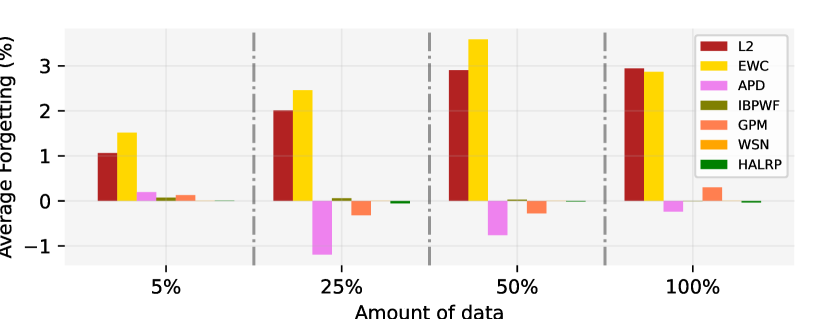
(a) Forgetting on 10 tasks of CIFAR100-Splits

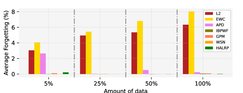
(b) Forgetting on 20 tasks in CIFAR100-SuperClass

Figure 2: Average Forgetting Statistics

5.5 Model Increment Analysis

Another potential issue in continual learning is the model size growth as the number of tasks increases. To compare increased model capacities among different methods, we visualize the ratio of increased parameters w.r.t to base model on the sequential 20 tasks of CIFAR100-Superclass dataset in Fig. 3(a). We can observe that our proposed HALRP can better control the model capacity increment. After the first four tasks, the model parameters are increased by around $19\%$ and grow slowly during the last sixteen tasks (finally $\leq 28\%$). In contrast, the model parameters of APD grew quickly by around $40\%$ in the first two or three tasks and keep a high ratio during the following tasks. Especially, we omit WSN as it adopted an extra binary mask compression procedure to reduce linear growth on the task-specific binary parameter masks, rather than directly considering the increase of parameter growth like most previous work.

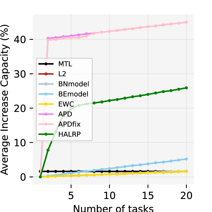
(a)

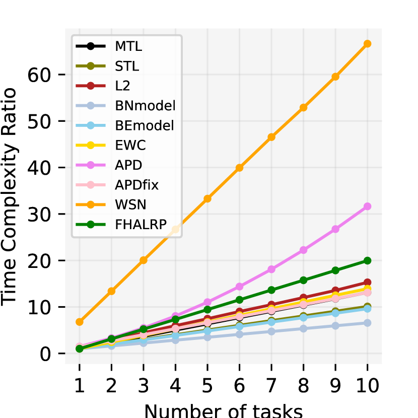
(b)

Figure 3: (a) Average Capacity Increment ratio on CIFAR100-Superclass w.r.t. the base model. (b) Average Time Complexity Ratio on PMNIST.

5.6 Computational Efficiency

We visualize the average time complexity ratio on the ten tasks of the PMNIST dataset in Fig. 3(b). The time complexity ratio is computed by dividing the accumulated time across the ten tasks w.r.t. the time cost on the first task of single-task learning. We observe that our proposed method introduces limited time consumption compared to most baselines, with a better trade-off between performance and efficiency. Especially, our method needs less training time compared to APD and WSN. The possible reason is that an extra time-consuming $k$-means clustering process is needed for the hierarchical knowledge consolidation among tasks in APD, while WSN needs to optimize the weight scores for each model parameter and then generate binary masks by locating the top-$c\%$ weight scores in the whole model.

5.7 Ablation Studies

We report the ablation study in Table V to evaluate further the impacts of the hyperparameters selection on performance using the CIFAR100 Splits dataset. We conduct the following ablations: (1) varying the warm-up epochs $n_{r}$, (2) varying the loss approximation rate $\alpha$, (3) LRP: omitting the importance estimation (step 6 of Algorithm 1), and (4) Random LRP: replacing step 6 of Algorithm 1 with a random decomposition. We can observe that the performance will not significantly rise as $n_{r}$ increases, which indicates that only one epoch is enough for warm-up training. When decreasing the approximate rate $\alpha$, the accuracy will decay. Furthermore, if we apply the random decomposition of the model, the accuracy will sharply drop, indicating the necessity of our Hessian aware-decomposition procedure.

Ablation	Acc.$\uparrow$	Size$\downarrow$
$\alpha$: 0.9, $n_{r}$: 1	$68.39\pm 0.13$	0.234
$\alpha$: 0.9, $n_{r}$: 2	$67.93\pm 0.19$	0.234
$\alpha$: 0.9, $n_{r}$: 3	$67.38\pm 0.12$	0.234
$\alpha$: 0.9, $n_{r}$: 4	$67.04\pm 0.08$	0.234
$\alpha$: 0.95, $n_{r}$: 1	$68.09\pm 0.15$	0.234
$\alpha$: 0.75, $n_{r}$: 1	$68.26\pm 0.11$	0.217
$\alpha$: 0.60, $n_{r}$: 1	$66.87\pm 0.23$	0.165
$\alpha$: 0.45, $n_{r}$: 1	$66.08\pm 0.14$	0.100
LRP.	$67.49\pm$ 0.13	0.234
Random LRP.	$61.76\pm 0.18$	0.235

TABLE V: Ablation studies. Acc.$\uparrow$ refers to the accuracy; Size refers to the relative increment size.

6 Conclusion

In this work, we propose a low-rank perturbation method for continual learning. Specifically, we approximate the task-adaptive parameters with low-rank decomposition by formulating the model transition along the sequential tasks with parameter transformations. We theoretically show the quantitative relationship between the Hessian and the proposed low-rank approximation, which leads to a novel Hessian-aware framework that enables the model to automatically select ranks by the relevant importance of the perturbation to the model’s performance. The extensive experimental results show that our proposed method performs better on the robustness of different task orders and the ability to address catastrophic forgetting issues.

Appendix A Background on Low-Rank Factorization for Matrix

Here, we provide more background knowledge about the low-rank matrix factorization.

In this work, we leverage the Eckart–Young–Mirsky theorem [35] with the Frobenius norm. In this part, we provide background knowledge for the self-cohesion of the paper.

Denote by ${\mathbf{B}\in\mathbb{R}^{m\times n}}$ a real (possibly rectangular) matrix. Suppose that $\mathbf{B}=\mathbf{U}\boldsymbol{\Sigma}\mathbf{V}^{\top}$ is the singular value decomposition (SVD) of $\mathbf{B}$, then, we can claim that the best rank $k$ approximation ($k\leq\min\{m,n\}$) to $\mathbf{B}$ under the Frobenius norm $\|\cdot\|_{F}$ is given by ${\mathbf{B}_{k}=\sum_{i=1}^{k}\sigma_{i}\mathbf{u}_{i}\mathbf{v}_{i}^{\top}}$, where $\mathbf{u}_{i}$ and $\mathbf{v}_{i}$ denote the $i^{th}$ column of $\mathbf{U}$ and $\mathbf{V}$, respectively. Then,

$$\|\mathbf{B}-\mathbf{B}_{k}\|_{F}^{2}=\Big{\|}\sum_{i=k+1}^{n}\sigma_{i}\mathbf{u}_{i}\mathbf{v}_{i}^{\top}\Big{\|}_{F}^{2}=\sum_{i=k+1}^{n}\sigma_{i}^{2}$$

Thus, we need to show that if $\mathbf{A}_{k}=XY^{\top}$ where $X$ and $Y$ has $k$ columns

$$\|\mathbf{B}-\mathbf{B}_{k}\|_{F}^{2}=\sum_{i=k+1}^{n}\sigma_{i}^{2}\leq\|\mathbf{B}-\mathbf{A}_{k}\|_{F}^{2}$$

.

By the triangle inequality, if $\mathbf{B}=\mathbf{B}^{\prime}+\mathbf{B}^{\prime\prime}$ then $\sigma_{1}(\mathbf{B})\leq\sigma_{1}(\mathbf{B}^{\prime})+\sigma_{1}(\mathbf{B}^{\prime\prime})$. Denote by $\mathbf{B}^{\prime}_{k}$ and $\mathbf{B}^{\prime\prime}_{k}$ the rank $k$ approximation to $\mathbf{B}^{\prime}$ and $\mathbf{B}^{\prime\prime}$ by the SVD method, respectively. Then, for any $i,j\geq 1$,

$$\begin{split}\sigma_{i}(\mathbf{B}^{\prime})+\sigma_{j}(\mathbf{B}^{\prime\prime})&=\sigma_{1}(\mathbf{B}^{\prime}-\mathbf{B}^{\prime}_{i-1})+\sigma_{1}(\mathbf{B}^{\prime\prime}-\mathbf{B}^{\prime\prime}_{j-1})\\ &\geq\sigma_{1}(\mathbf{B}-\mathbf{B}^{\prime}_{i-1}-\mathbf{B}^{\prime\prime}_{j-1})\\ &\geq\sigma_{1}(\mathbf{B}-\mathbf{B}_{i+j-2})\qquad\\ &=\sigma_{i+j-1}(\mathbf{B})\end{split}$$

where the last inequality comes from the fact that ${\rm{rank}}(\mathbf{B}^{\prime}_{i-1}+\mathbf{B}^{\prime\prime}_{j-1})\leq{\rm{rank\,}}(\mathbf{B}_{i+j-2})$.

Since $\sigma_{k+1}(\mathbf{B}_{k})=0$, when $\mathbf{B}^{\prime}=\mathbf{B}-\mathbf{A}_{k}$ and $\mathbf{B}^{\prime\prime}=\mathbf{A}_{k}$ we conclude that for $i\geq 1,j=k+1$

$$\sigma_{i}(\mathbf{B}-\mathbf{A}_{k})\geq\sigma_{k+i}(\mathbf{B})$$

Therefore,

$$\begin{split}\|\mathbf{B}-\mathbf{A}_{k}\|_{F}^{2}=&\sum_{i=1}^{n}\sigma_{i}(\mathbf{B}-\mathbf{A}_{k})^{2}\geq\sum_{i=k+1}^{n}\sigma_{i}(\mathbf{B})^{2}=\|\mathbf{B}-\mathbf{B}_{k}\|_{F}^{2}\end{split}$$

Thus, we can get Eq. 1 displayed in the paper.

Appendix B Proof to Theorem 1 and Discussion

Theorem 2.

Assume that a neural network of $L$ layers with vectorized weights $(\boldsymbol{\omega}^{\star}_{1},\dots,\boldsymbol{\omega}^{\star}_{L})$ that have converged to local optima, such that the first and second order optimality conditions are satisfied, i.e., the gradient is zero, and the Hessian is positive semi-definite. Suppose a perturbation $\Delta\boldsymbol{\omega}^{\star}_{1}$ applied to the first layer weights, then we have the loss increment

$$\begin{split}\mathcal{L}(\boldsymbol{\omega}^{\star}_{1}-\Delta\boldsymbol{\omega}^{\star}_{1},&\dots,\boldsymbol{\omega}^{\star}_{L})-\mathcal{L}(\boldsymbol{\omega}^{\star}_{1},\dots,\boldsymbol{\omega}^{\star}_{L})\\ &\leq\|\frac{1}{2}\mathbf{H}_{1}\|_{F}\|\Delta\boldsymbol{\omega}^{\star}_{1}\|^{2}_{F}+o(\|\Delta\boldsymbol{\omega}^{\star}_{1}\|^{2}_{F}),\end{split}$$ (14)

where $\mathbf{H}_{1}=\Delta\mathcal{L}(\boldsymbol{\omega}^{\star}_{1})$ is the Hessian matrix at only the variables of the first layer weights.

Proof.

Denote the gradient and Hessian of the first layer $\boldsymbol{\omega}^{\star}_{1}$ as $\mathbf{g}_{1}$ and $\mathbf{H}_{1}$. Through Taylor’s expansion, we have

$$\begin{split}\mathcal{L}(\boldsymbol{\omega}^{\star}_{1}&-\Delta\boldsymbol{\omega}^{\star}_{1},\dots,\boldsymbol{\omega}^{\star}_{L})-\mathcal{L}(\boldsymbol{\omega}^{\star}_{1},\dots,\boldsymbol{\omega}^{\star}_{L})\\ &=-\mathbf{g}_{1}^{T}\Delta\boldsymbol{\omega}^{\star}_{1}+\frac{1}{2}\Delta\boldsymbol{\omega}^{\star T}_{1}\mathbf{H}_{1}\Delta\boldsymbol{\omega}^{\star}_{1}+o(\|\Delta\boldsymbol{\omega}^{\star}_{1}\|^{2}_{F}).\end{split}$$

Using the fact that the gradient is zero at the local optimum $\boldsymbol{\omega}^{\star}_{1}$ as well as the sub-additive and sub-multiplicative properties of Frobenius norm, we have,

$$\begin{split}\mathcal{L}(\boldsymbol{\omega}^{\star}_{1}&-\Delta\boldsymbol{\omega}^{\star}_{1},\dots,\boldsymbol{\omega}^{\star}_{L})-\mathcal{L}(\boldsymbol{\omega}^{\star}_{1},\dots,\boldsymbol{\omega}^{\star}_{L})\\ &=\frac{1}{2}\Delta\boldsymbol{\omega}^{\star T}_{1}\mathbf{H}_{1}\Delta\boldsymbol{\omega}^{\star}_{1}+o(\|\Delta\boldsymbol{\omega}^{\star}_{1}\|^{2}_{F})\\ &=\|\frac{1}{2}\Delta\boldsymbol{\omega}^{\star T}_{1}\mathbf{H}_{1}\Delta\boldsymbol{\omega}^{\star}_{1}+o(\|\Delta\boldsymbol{\omega}^{\star}_{1}\|^{2}_{F})\|_{F}\\ &\leq\|\frac{1}{2}\Delta\boldsymbol{\omega}^{\star T}_{1}\mathbf{H}_{1}\Delta\boldsymbol{\omega}^{\star}_{1}\|_{F}+o(\|\Delta\boldsymbol{\omega}^{\star}_{1}\|^{2}_{F})\\ &\leq\|\frac{1}{2}\mathbf{H}_{1}\|_{F}\|\Delta\boldsymbol{\omega}^{\star}_{1}\|^{2}_{F}+o(\|\Delta\boldsymbol{\omega}^{\star}_{1}\|^{2}_{F}).\end{split}$$

Thus, we conclude the proof.

∎

Algorithm 1 implies that the Hessian information can be used to quantitatively measure the influences of low-rank perturbation on the model’s empirical losses. In practice, we can approximate the Hessian by the negative empirical Fisher information [40]. This enables a dynamic scheme for the trade-off between the approximation error and computational efficiency. For a given loss approximation rate, the model can automatically select the rank for all the layers.

Appendix C Discussion on the Fine-tuning Objective on the New Task

In the proposed algorithm, we finally fine-tune the model on the new task with Eq. 12 in the manuscript, which is re-illustrated below,

$$\min_{\mathbf{W}_{t}}\mathcal{L}(\mathbf{W}_{t};\mathcal{D}_{t})+\mathcal{L}_{\text{reg}}(\mathbf{W}_{t};\mathcal{D}_{t})$$ (15)

where

$$\mathcal{L}_{\text{reg}}(\mathbf{W}_{t};\mathcal{D}_{t})=\sum_{l} \Big{[}+\lambda_{0}\underbrace{(\|\mathbf{U}_{i}^{(k_{l})\text{free}}\|+\|\mathbf{V}_{i}^{(k_{l})\text{free}}\|)}_{L_{1}-\mathrm{regularization}}$$ (16)

$$+\lambda_{1}\underbrace{(\|\mathbf{R}_{i}^{\text{free}}\|_{2}^{2}+\|\mathbf{S}_{i}^{\text{free}}\|_{2}^{2})}_{L_{2}-\mathrm{regularization}}$$

$$+\lambda_{2}\underbrace{(\|\mathbf{U}_{i}^{(k_{l})\text{free}}\|_{2}^{2}+\|\mathbf{V}_{i}^{(k_{l})\text{free}}\|_{2}^{2})}_{L_{2}-\mathrm{regularization}}\Big{]}$$

The fine-tuning objective mainly consists of three parts, the general cross-entropy loss on the new task $\mathcal{T}_{t}$, a $L_{1}$ regularization term on $\|\mathbf{U}_{i}^{(k_{l})\text{free}}\|+\|\mathbf{V}_{i}^{(k_{l})\text{free}}\|$, and the $L_{2}$ regularization terms on $\|\mathbf{R}_{i}^{\text{free}}\|_{2}^{2}+\|\mathbf{S}_{i}^{\text{free}}\|_{2}^{2}$ and $\|\mathbf{U}_{i}^{(k_{l})\text{free}}\|_{2}^{2}+\|\mathbf{V}_{i}^{(k_{l})\text{free}}\|_{2}^{2}$, respectively.

As mentioned in the paper, we apply the $L_{1}$ regularization on $\mathbf{U}_{i}^{(k_{l})\text{free}}$ and $\mathbf{V}_{i}^{(k_{l})\text{free}}$. Besides, as discussed in Section 4.4 of the paper, we also apply to prune $\mathbf{U}_{i}^{\text{free}}$ and $\mathbf{V}_{i}^{(k_{l})\text{free}}$, which further encouraged the sparsity.

Our method keeps $\mathbf{W}^{\text{base}}$ as unchanged for new tasks for knowledge transfer, while the $\mathbf{R}_{i}^{\text{free}}$, $\mathbf{S}_{i}^{\text{free}}$, $\mathbf{U}_{i}^{(k)\text{free}}$ and $\mathbf{V}_{i}^{(k)\text{free}}$ are left as task-adaptive parameters. Since $\mathbf{R}_{i}^{\text{free}}$ and $\mathbf{S}_{i}^{\text{free}}$ are diagonal matrices, plus the fact that $\mathbf{U}_{i}^{(k)\text{free}}$ and $\mathbf{V}_{i}^{(k)\text{free}}$ are sparse, thus the model only needs to learn a small number of parameters. Unlike some regularization methods (e.g. EWC [4]), which constrain the gradient update and require to re-train a lot of parameters, our method can update the model more efficiently. In addition, the empirical results reported in the paper show that our method can also achieve better performance with less time and memory cost.

Appendix D Additional Experimental Results

	PMNIST-20 (MLP)	CIFAR100-20 (ResNet18)	CIFAR100-20 (MLP)
Multitask($\star$)	$96.8$	$70.2$	$16.4$
IRU($\star$)	$85.60\pm 0.15$	$68.46\pm 2.52$	$65.90\pm 2.16$
Ours	$92.02\pm 0.04$	$73.71\pm 0.87$	$67.21\pm 0.68$

TABLE VI: Comparison under the IRU [33] setting. Results with $\star$ are from IRU paper.

	P-MNIST
	Acc.$\uparrow$	MOPD$\downarrow$	AOPD$\downarrow$
IBWPF	78.12 $\pm$ 0.83	12.69	6.65
HALRP	98.10 $\pm$ 0.03	0.47	0.24
	Five-dataset
	Acc.$\uparrow$	MOPD$\downarrow$	AOPD$\downarrow$
IBWPF	84.62 $\pm$ 0.36	5.06	1.72
HALRP	88.81 $\pm$ 0.31	4.28	1.31

TABLE VII: Comparison with low-rank factorization method

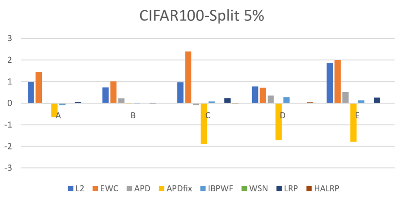
(a) 5% of training data

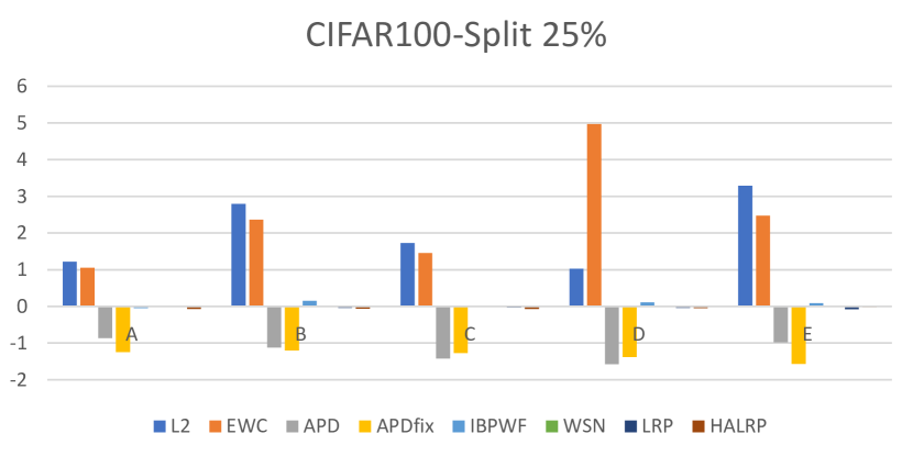
(b) 25% of training data

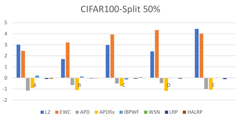
(c) 50% of training data

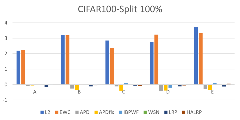
(d) 100% of training data

Figure 4: Forgetting comparison on CIFAR100-Split with different task orders (A-E) under different amounts of training data.

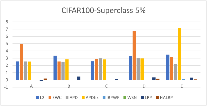
(a) 5% of training data

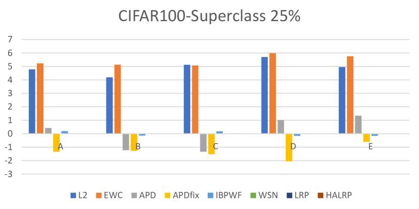
(b) 25% of training data

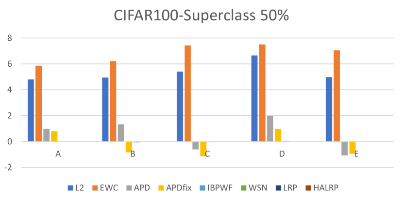
(c) 50% of training data

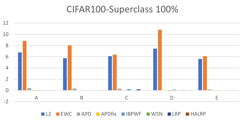
(d) 100% of training data

Figure 5: Forgetting on CIFAR100-Superclass with different task orders (A-E) under different amounts of training data.

D.1 Comparing with other low-rank methods

We note that the official code of IRU [33] only contains a demo for multi-layer perceptron (MLP), and no complete code for the convolutional network (even LeNet) can be found. Due to this limitation, we re-implement our method under the setting of IRU [33] to make a fair comparison in Table VI. We describe the IRU setting as follows: (1) Dataset Protocol: [33] generated 20 random tasks on PMNIST, rather than 10 tasks in this work. Moreover, [33] randomly divided the CIFAR100 dataset into 20 tasks, rather than the superclass-based splitting in our paper. Thus, we denote the two datasets in [33] as “PMNIST-20” and “CIFAR100-20” in Table VI, to distinguish from the “PMNIST” and “CIFAR100-Superclass” used in the common setting. (2) Model Architecture: The “MLP” in Table VI indicates the three-layer (fully-connected) multilayer perceptron with 256 hidden nodes. From Table VI, we can conclude that our HALRP outperforms IRU under different datasets and networks.

Our work also shares some similarities with the low-rank-decomposition-based method IBPWF [10]. As discussed in [33] and in our paper (Sec. 1), this method requires larger ranks to accept higher accuracy. Furthermore, as pointed out by [50], IBPWF leverages Bayesian non-parametric to let the data dictate expansion, but the benchmarks considered in Bayesian methods have been limited to smaller datasets, like MNIST and CIFAR-10. In addition to the experimental comparisons with IBPWF reported in the paper, we further report more results in Table VII. We can observe that our method outperforms IBPWF with a large gap in terms of Accuracy and MOPD$\downarrow$ & AOPD$\downarrow$. Furthermore, we observe that IBPWF cannot perform well on P-MNIST, which is $10\times$ the number of data of MNIST. The gap is consistent with observations in [50].

D.2 Performance on Alleviate Forgetting on Different Task Orders

In the main paper, we report the forgetting performance on the average of five task orders (A-E) on CIFAR-100 Splits and Superclass. In this part, we provide the performance on forgetting under each task order in Fig. 4 and Fig. 5, under different amounts (i.e., $5\%\sim 100\%$) of training data from.

Appendix E Experimental Details

E.1 Dataset Preparation

CIFAR-100 Splits/SuperClass We used the CIFAR-100 Splits/Superclass dataset following the evaluation protocol of [9], and follow the task order definition of [9] to test the algorithms with five different task orders (A-E).

For the CIFAR-100 split, the task orders are defined as:

• Order A: [0,1,2,3,4,5,6,7,8,9]

• Order B: [1, 7, 4, 5, 2, 0, 8, 6, 9, 3]

• Order C: [7, 0, 5, 1, 8, 4, 3, 6, 2, 9]

• Order D: [5, 8, 2, 9, 0, 4, 3, 7, 6, 1]

• Order E: [2, 9, 5, 4, 8, 0, 6, 1, 3, 7]

For the CIFAR-100 Superclass, the task orders are:

• Order A: [0, 1, 2, 3, 4, 5, 6, 7, 8, 9, 10, 11, 12, 13, 14, 15, 16, 17, 18, 19]

• Order B: [15, 12, 5, 9, 7, 16, 18, 17, 1, 0, 3, 8, 11, 14, 10, 6, 2, 4, 13, 19]

• Order C: [17, 1, 19, 18, 12, 7, 6, 0, 11, 15, 10, 5, 13, 3, 9, 16, 4, 14, 2, 8]

• Order D: [11, 9, 6, 5, 12, 4, 0, 10, 13, 7, 14, 3, 15, 16, 8, 1, 2, 19, 18, 17]

• Order E: [6, 14, 0, 11, 12, 17, 13, 4, 9, 1, 7, 19, 8, 10, 3, 15, 18, 5, 2, 16]

Furthermore, as discussed in the paper, we demonstrate the performance when handling limited training data. In this regard, we randomly select $5\%$, $25\%$, $50\%$ training data from each task and report the corresponding accuracies.

P-MNIST We follow [19] to evaluate the algorithms’ performance on the P-MNIST dataset. Each task of P-MNIST is a random permutation of the original MNIST pixel. We follow [19, 41] to generate the train/val/test splits and to create 10 sequential tasks using different permutations, and each task has 10 classes. We randomly generate five different task orders with five different seeds.

Five dataset It uses a sequence of 5 different benchmarks including CIFAR10 [42], MNIST [43], notMNIST [44], FashionMNIST [45] and SVHN [46]. Each benchmark contains 10 classes. We follow [19] to generate the train/val/test splits and to create 10 sequential tasks using different permutations, and each task has 10 classes. We randomly generate five different task orders with five different seeds.

Omniglot-rotation Omniglot [47] consists of 100 12-way classification tasks. We follow the train/val/test split of [19].

E.2 Model Architecture

In the experimental evaluations, we implement various kinds of backbone architectures to demonstrate our perturbation method for different deep models. We introduce the model architectures used in the paper

LeNet We implement two kinds of LeNet models: 1): For CIFAR-100 Splits/Superclass (Table 1 & Table 3), and P-MNIST (Table 2 (a)), we implement the general LeNet model with neurons 20-20-50-800-500-10. 2): For Omniglot-Rotation (Table 2 (c)), we follow [9, 19] to implement the enlarged LeNet model with neurons 64-128-2500-1500.

AlexNet For the experiments on Five-dataset (Table 2(b)), we implement AlexNet model by following [2, 19].

ResNet-18 We implement a reduced ResNet-18 model on the Five-dataset (Table 2(b)) by following [19].

Dataset	CIFAR-100 Split	CIFAR-100 Super	PMNIST	Five dataset	Omniglot
$n$	20	20	12	12	20
$n_{r}$	1	1	1	1	1
$\alpha$	0.9	0.9	0.9	0.9	0.99
LR	$10^{-3}$	$10^{-3}$	$10^{-3}$	$10^{-3}$	$5\times 10^{-3}$
$\lambda_{0}$	$10^{-6}$	$10^{-6}$	$10^{-6}$	$10^{-6}$	$9\times 10^{-5}$
$\lambda_{1}$	$10^{-4}$	$10^{-4}$	$10^{-3}$	$10^{-4}$	$10^{-4}$
$\lambda_{2}$	$10^{-4}$	$1\times 10^{-4}$	$10^{-3}$	$10^{-4}$	$10^{-4}$
Bcsz	128	128	128	128	16

TABLE VIII: Hyperparameters for the experiments. $n$: total epoch. $n_{r}$: warm-up epochs for a new task. LR: Learning rate. $\lambda_{0},\lambda_{1},\lambda_{2}$: coefficients for the regularization terms as discussed in Appendix C. Bcsz: training batch size.

E.3 Training Hyperparameters

We reimplement the baselines by rigorously following the official code release or publicly accessible implementations and tested our proposed algorithm with a unified test-bed with the same hyperparameters to get fair comparison results. The training details for our experiments are illustrated in Table VIII. The hyperparameters are selected via grid search. We also provide descriptions of the hyperparameters in the source code.

References

- [1] M. De Lange, R. Aljundi, M. Masana, S. Parisot, X. Jia, A. Leonardis, G. Slabaugh, and T. Tuytelaars, “A continual learning survey: Defying forgetting in classification tasks,” IEEE transactions on pattern analysis and machine intelligence, vol. 44, no. 7, pp. 3366–3385, 2021.
- [2] G. Saha, I. Garg, and K. Roy, “Gradient projection memory for continual learning,” in International Conference on Learning Representations, 2021. [Online]. Available: https://openreview.net/forum?id=3AOj0RCNC2
- [3] M. Farajtabar, N. Azizan, A. Mott, and A. Li, “Orthogonal gradient descent for continual learning,” in International Conference on Artificial Intelligence and Statistics. PMLR, 2020, pp. 3762–3773.
- [4] J. Kirkpatrick, R. Pascanu, N. Rabinowitz, J. Veness, G. Desjardins, A. A. Rusu, K. Milan, J. Quan, T. Ramalho, A. Grabska-Barwinska et al., “Overcoming catastrophic forgetting in neural networks,” Proceedings of the national academy of sciences, vol. 114, no. 13, pp. 3521–3526, 2017.
- [5] S. Jung, H. Ahn, S. Cha, and T. Moon, “Continual learning with node-importance based adaptive group sparse regularization,” Advances in Neural Information Processing Systems, vol. 33, pp. 3647–3658, 2020.
- [6] M. K. Titsias, J. Schwarz, A. G. d. G. Matthews, R. Pascanu, and Y. W. Teh, “Functional regularisation for continual learning with gaussian processes,” arXiv preprint arXiv:1901.11356, 2019.
- [7] S. Wang, X. Li, J. Sun, and Z. Xu, “Training networks in null space of feature covariance for continual learning,” in Proceedings of the IEEE/CVF conference on Computer Vision and Pattern Recognition, 2021, pp. 184–193.
- [8] Y. Kong, L. Liu, H. Chen, J. Kacprzyk, and D. Tao, “Overcoming catastrophic forgetting in continual learning by exploring eigenvalues of hessian matrix,” IEEE Transactions on Neural Networks and Learning Systems, pp. 1–15, 2023.
- [9] J. Yoon, S. Kim, E. Yang, and S. J. Hwang, “Scalable and order-robust continual learning with additive parameter decomposition,” in 8th International Conference on Learning Representations, ICLR 2020, Addis Ababa, Ethiopia, April 26-30, 2020. OpenReview.net, 2020. [Online]. Available: https://openreview.net/forum?id=r1gdj2EKPB
- [10] N. Mehta, K. Liang, V. K. Verma, and L. Carin, “Continual learning using a bayesian nonparametric dictionary of weight factors,” in International Conference on Artificial Intelligence and Statistics. PMLR, 2021, pp. 100–108.
- [11] Y. Wen, D. Tran, and J. Ba, “Batchensemble: an alternative approach to efficient ensemble and lifelong learning,” in 8th International Conference on Learning Representations, ICLR 2020, Addis Ababa, Ethiopia, April 26-30, 2020. OpenReview.net, 2020. [Online]. Available: https://openreview.net/forum?id=Sklf1yrYDr
- [12] J. Serra, D. Suris, M. Miron, and A. Karatzoglou, “Overcoming catastrophic forgetting with hard attention to the task,” in International conference on machine learning. PMLR, 2018, pp. 4548–4557.
- [13] A. Chaudhry, N. Khan, P. Dokania, and P. Torr, “Continual learning in low-rank orthogonal subspaces,” Advances in Neural Information Processing Systems, vol. 33, pp. 9900–9911, 2020.
- [14] Y. Yang, Z.-Q. Sun, H. Zhu, Y. Fu, Y. Zhou, H. Xiong, and J. Yang, “Learning adaptive embedding considering incremental class,” IEEE Transactions on Knowledge and Data Engineering, vol. 35, no. 3, pp. 2736–2749, 2023.
- [15] A. A. Rusu, N. C. Rabinowitz, G. Desjardins, H. Soyer, J. Kirkpatrick, K. Kavukcuoglu, R. Pascanu, and R. Hadsell, “Progressive neural networks,” arXiv preprint arXiv:1606.04671, 2016.
- [16] J. Yoon, E. Yang, J. Lee, and S. J. Hwang, “Lifelong learning with dynamically expandable networks,” in Proceedings of International Conference on Learning Representations, 2017.
- [17] X. Li, Y. Zhou, T. Wu, R. Socher, and C. Xiong, “Learn to grow: A continual structure learning framework for overcoming catastrophic forgetting,” in International Conference on Machine Learning. PMLR, 2019, pp. 3925–3934.
- [18] A.-A. Liu, H. Lu, H. Zhou, T. Li, and M. Kankanhalli, “Balanced class-incremental 3d object classification and retrieval,” IEEE Transactions on Knowledge and Data Engineering, pp. 1–13, 2023.
- [19] H. Kang, R. J. L. Mina, S. R. H. Madjid, J. Yoon, M. Hasegawa-Johnson, S. J. Hwang, and C. D. Yoo, “Forget-free continual learning with winning subnetworks,” in International Conference on Machine Learning. PMLR, 2022, pp. 10 734–10 750.
- [20] M. Riemer, I. Cases, R. Ajemian, M. Liu, I. Rish, Y. Tu, and G. Tesauro, “Learning to learn without forgetting by maximizing transfer and minimizing interference,” arXiv preprint arXiv:1810.11910, 2018.
- [21] S.-A. Rebuffi, A. Kolesnikov, G. Sperl, and C. H. Lampert, “icarl: Incremental classifier and representation learning,” in Proceedings of the IEEE conference on Computer Vision and Pattern Recognition, 2017, pp. 2001–2010.
- [22] B. Zhang, Y. Guo, Y. Li, Y. He, H. Wang, and Q. Dai, “Memory recall: A simple neural network training framework against catastrophic forgetting,” IEEE Transactions on Neural Networks and Learning Systems, vol. 33, no. 5, pp. 2010–2022, 2022.
- [23] H. Chen, Y. Wang, and Q. Hu, “Multi-granularity regularized re-balancing for class incremental learning,” IEEE Transactions on Knowledge and Data Engineering, vol. 35, no. 7, pp. 7263–7277, 2023.
- [24] G. Sun, Y. Cong, Y. Zhang, G. Zhao, and Y. Fu, “Continual multiview task learning via deep matrix factorization,” IEEE Transactions on Neural Networks and Learning Systems, vol. 32, no. 1, pp. 139–150, 2021.
- [25] S. Ho, M. Liu, L. Du, L. Gao, and Y. Xiang, “Prototype-guided memory replay for continual learning,” IEEE Transactions on Neural Networks and Learning Systems, 2023.
- [26] L. Wang, B. Lei, Q. Li, H. Su, J. Zhu, and Y. Zhong, “Triple-memory networks: A brain-inspired method for continual learning,” IEEE Transactions on Neural Networks and Learning Systems, vol. 33, no. 5, pp. 1925–1934, 2021.
- [27] A. Chaudhry, M. Ranzato, M. Rohrbach, and M. Elhoseiny, “Efficient lifelong learning with a-gem,” International Conference on Learning Representations, 2019.
- [28] C. Tai, T. Xiao, X. Wang, and W. E, “Convolutional neural networks with low-rank regularization,” in 4th International Conference on Learning Representations, ICLR 2016, San Juan, Puerto Rico, May 2-4, 2016, Conference Track Proceedings, Y. Bengio and Y. LeCun, Eds., 2016. [Online]. Available: http://arxiv.org/abs/1511.06067
- [29] Y. Idelbayev and M. A. Carreira-Perpinán, “Low-rank compression of neural nets: Learning the rank of each layer,” in Proceedings of the IEEE/CVF Conference on Computer Vision and Pattern Recognition, 2020, pp. 8049–8059.
- [30] A.-H. Phan, K. Sobolev, K. Sozykin, D. Ermilov, J. Gusak, P. Tichavskỳ, V. Glukhov, I. Oseledets, and A. Cichocki, “Stable low-rank tensor decomposition for compression of convolutional neural network,” in European Conference on Computer Vision. Springer, 2020, pp. 522–539.
- [31] L. Wang, M. Rege, M. Dong, and Y. Ding, “Low-rank kernel matrix factorization for large-scale evolutionary clustering,” IEEE Transactions on Knowledge and Data Engineering, vol. 24, no. 6, pp. 1036–1050, 2012.
- [32] X. Zhu, S. Zhang, Y. Li, J. Zhang, L. Yang, and Y. Fang, “Low-rank sparse subspace for spectral clustering,” IEEE Transactions on Knowledge and Data Engineering, vol. 31, no. 8, pp. 1532–1543, 2019.
- [33] R. Hyder, K. Shao, B. Hou, P. Markopoulos, A. Prater-Bennette, and M. S. Asif, “Incremental task learning with incremental rank updates,” in European Conference on Computer Vision. Springer, 2022, pp. 566–582.
- [34] M. P. Deisenroth, A. A. Faisal, and C. S. Ong, Mathematics for machine learning. Cambridge University Press, 2020.
- [35] C. Eckart and G. Young, “The approximation of one matrix by another of lower rank,” Psychometrika, vol. 1, no. 3, pp. 211–218, 1936.
- [36] C. R. Harris, K. J. Millman, S. J. van der Walt, R. Gommers, P. Virtanen, D. Cournapeau, E. Wieser, J. Taylor, S. Berg, N. J. Smith, R. Kern, M. Picus, S. Hoyer, M. H. van Kerkwijk, M. Brett, A. Haldane, J. F. del Río, M. Wiebe, P. Peterson, P. Gérard-Marchant, K. Sheppard, T. Reddy, W. Weckesser, H. Abbasi, C. Gohlke, and T. E. Oliphant, “Array programming with NumPy,” Nature, vol. 585, no. 7825, pp. 357–362, Sep. 2020. [Online]. Available: https://doi.org/10.1038/s41586-020-2649-2
- [37] A. Paszke, S. Gross, S. Chintala, G. Chanan, E. Yang, Z. DeVito, Z. Lin, A. Desmaison, L. Antiga, and A. Lerer, “Automatic differentiation in pytorch,” 2017.
- [38] Z. Dong, Z. Yao, A. Gholami, M. W. Mahoney, and K. Keutzer, “Hawq: Hessian aware quantization of neural networks with mixed-precision,” in Proceedings of the IEEE/CVF International Conference on Computer Vision, 2019, pp. 293–302.
- [39] Z. Dong, Z. Yao, D. Arfeen, A. Gholami, M. W. Mahoney, and K. Keutzer, “Hawq-v2: Hessian aware trace-weighted quantization of neural networks,” Advances in neural information processing systems, vol. 33, pp. 18 518–18 529, 2020.
- [40] F. Kunstner, P. Hennig, and L. Balles, “Limitations of the empirical fisher approximation for natural gradient descent,” Advances in neural information processing systems, vol. 32, 2019.
- [41] S. Ebrahimi, M. Elhoseiny, T. Darrell, and M. Rohrbach, “Uncertainty-guided continual learning with bayesian neural networks,” arXiv preprint arXiv:1906.02425, 2019.
- [42] A. Krizhevsky, G. Hinton et al., “Learning multiple layers of features from tiny images,” 2009.
- [43] L. Deng, “The mnist database of handwritten digit images for machine learning research,” IEEE Signal Processing Magazine, vol. 29, no. 6, pp. 141–142, 2012.
- [44] Y. Bulatov, “Notmnist dataset. google (books/ocr),” Tech. Rep.[Online]. Available: http://yaroslavvb. blogspot. it/2011/09 …, Tech. Rep., 2011.
- [45] H. Xiao, K. Rasul, and R. Vollgraf. (2017) Fashion-mnist: a novel image dataset for benchmarking machine learning algorithms.
- [46] N. Yuval, W. Tao, C. Adam, B. Alessandro, W. Bo, and N. Andrew Y., “Reading digits in natural images with unsupervised feature learning,” in In Proceedings of NIPS Workshop on Deep Learning and Unsupervised Feature Learning. PMLR, 2011, pp. 522–539.
- [47] B. M. Lake, R. Salakhutdinov, and J. B. Tenenbaum, “Human-level concept learning through probabilistic program induction,” Science, vol. 350, no. 6266, pp. 1332–1338, 2015.
- [48] Y. Zhang and Q. Yang, “A survey on multi-task learning,” IEEE Transactions on Knowledge and Data Engineering, vol. 34, no. 12, pp. 5586–5609, 2022.
- [49] S. Ioffe and C. Szegedy, “Batch normalization: Accelerating deep network training by reducing internal covariate shift,” in International conference on machine learning. PMLR, 2015, pp. 448–456.
- [50] V. K. Verma, K. J. Liang, N. Mehta, P. Rai, and L. Carin, “Efficient feature transformations for discriminative and generative continual learning,” in Proceedings of the IEEE/CVF Conference on Computer Vision and Pattern Recognition, 2021, pp. 13 865–13 875.