Angular-Distance Based Channel Estimation for Holographic MIMO
Abstract
Leveraging the concept of the electromagnetic signal and information theory, holographic multiple-input multiple-output (MIMO) technology opens the door to an intelligent and endogenously holography-capable wireless propagation environment, with their unparalleled capabilities for achieving high spectral and energy efficiency. Less examined are the important issues such as the acquisition of accurate channel information by accounting for holographic MIMO’s peculiarities. To fill this knowledge gap, this paper investigates the channel estimation for holographic MIMO systems by unmasking their distinctions from the conventional one. Specifically, we elucidate that the channel estimation, subject to holographic MIMO’s electromagnetically large antenna arrays, has to discriminate not only the angles of a user/scatterer but also its distance information, namely the three-dimensional (3D) azimuth and elevation angles plus the distance (AED) parameters. As the angular-domain representation fails to characterize the sparsity inherent in holographic MIMO channels, the tightly coupled 3D AED parameters are firstly decomposed for independently constructing their own covariance matrices. Then, the recovery of each individual parameter can be structured as a compressive sensing (CS) problem by harnessing the covariance matrix constructed. This pair of techniques contribute to a parametric decomposition and compressed deconstruction (DeRe) framework, along with a formulation of the maximum likelihood estimation for each parameter. Then, an efficient algorithm, namely DeRe-based variational Bayesian inference and message passing (DeRe-VM), is proposed for the sharp detection of the 3D AED parameters and the robust recovery of sparse channels. Finally, the proposed channel estimation regime is confirmed to be of great robustness in accommodating different channel conditions, regardless of the near-field and far-field contexts of a holographic MIMO system, as well as an improved performance in comparison to the state-of-the-art benchmarks.
Index Terms:
Holographic MIMO, electromagnetic signal, channel estimation, near-field communications.I Introduction
The paradigm shift from the fifth-generation (5G) to the sixth-generation (6G) communications catalyzes pillar functionalities shared among plethora of newly encountered particularities, with critical performance metrics to be placated including but not subject to ultra-wideband, ultra-massive access, ultra-reliability, and low latency [1, 2, 3]. As a “holly grail” of wireless technologies, massive multi-input and multi-output (mMIMO) has non-trivial capabilities of achieving unprecedented spectral efficiency, the critical ingredients of which have been commercially rolled out and approved for inclusion in 5G next radio (NR) standards [4]. While looking back from MIMO, mMIMO, to the more recent extremely large-scale (XL) MIMO, one may notice that all three adhere to the same philosophy, namely to adapt to an uncontrollable wireless environment. Their beamforming functionalities conform to the beam-space model in the specific domain based upon a number of ideal assumptions, e.g., predefined antenna array geometry with explicit calibrations, along with propagation in the absence of near-field scattering and mutual coupling [5, 6, 7, 8, 9]. This would be fruitless as the array aperture becomes larger and electromagnetically manipulated, shaped in arbitrary geometries and covered with dense antenna elements. Therefore, we are highly anticipating the evolution of the classical signal processing methodologies to the electromagnetic (EM) level using EM signal and information theory, allowing for greater degrees of freedom in the context of 6G [10].
Benefiting from the advancement of meta-materials and meta-surfaces, along with their widespread uses in wireless communications, holographic MIMO has been crafted as an excellent candidate to enable holographic radios. The fundamentals of holographic MIMO have been expounded in [11, 12, 13], and herein we will shine the spotlight on the qualitative leaps from the conventional MIMO to its holographic counterpart for the following twofold aspects. Firstly, regarding physical fundamentals, holographic MIMO is considered to have a nearly continuous aperture with antenna element spacing being much less than half a wavelength of incident EM waves. This contrasts with the half-wavelength condition typical in conventional MIMO. Such a distinction leads to transformative changes in hardware structure, notably in terms of the array aperture size (from small to extremely large) and the number/density of antenna elements (from sparse to dense). Intriguingly, the densely packed antenna elements may lead to enhancement in spectral efficiency [14]. Furthermore, the attendant mutual coupling among antenna elements, albeit deemed detrimental in conventional MIMO designs, fundamentally transforms, and is potential to be leveraged in achieving the super-directivity, a phenomenon that describes the significantly higher array gains obtained in holographic MIMO [15, 16]. Secondly, from the perspective of propagation channels, another qualitative change in holographic MIMO results from its extremely large aperture size. Unlike mMIMO communications that typically employ planar wavefront in far-field cases, holographic MIMO can naturally draw the far-field region to its near-field counterpart (also known as the Fresnel region) as the aperture size increases. Therefore, holographic MIMO near-field communications have to discriminate not only the angle of a scatterer but also its distance information, in contrast to the angle-only-aware counterpart in mMIMO systems.
Given that holographic MIMO just plays a basic physical role, associated physical-layer technologies are required for further implementation of holographic communications. To this end, significant efforts have been devoted to the channel modeling [17, 18, 19, 20, 21], channel estimation [19, 22], and holographic beampattern design [23, 24, 25]. In these literatures, the holographic channel models employed might not arrive at a good consensus, which can be roughly classified into two categories: i) EM channel based on Fourier planar wavefront representation [17, 20, 21], and ii) parametric physical channel based on multi-path representation [22, 26]. More precisely, the former goes more deeply into characterizing what kind of channel distributions that could appear in the radiative near-field and what cannot. The latter is more concentrated on the imposed sparsity in the sense that the received signal contains a sum of a few spherical waves, based upon which the compressive sensing (CS) method can be harnessed for facilitating high-efficiency parameter recovery. In spite of this, we believe that this pair of somewhat different channel models for characterizing holographic MIMO may be aligned to the same ingredients but using different methods for analyzing the holographic MIMO channels.
Holographic MIMO’s intriguing features contribute significantly to the achievement of holographic radios, yet just a few fledgling efforts on channel estimation in the true sense of the term are available to date, e.g., [19, 22]. Even so, we are fortunate to observe, as more attention is drawn to related topics, the emergence of pioneering studies with a focus on near-field channel estimation based on the assumption of spherical wavefront utilizing various techniques [22, 26, 27, 28, 29], such as CS-based approaches [26, 29], and learning-based means [28]. In particular, the potential sparsity intrinsic to the near-field channel has been unveiled in [26], where a polar-domain representation is proposed in lieu of the angular-domain counterpart in the far field. Base upon the polar-domain philosophy, the near-field codebook solution is devised in [27] for multiple access. In [29], a joint dictionary learning and sparse recovery empowered channel estimation is presented for near-field communications. Furthermore, in a distinct approach, a model-based deep learning framework for near-field channel estimation is showcased in [28], in which the channel estimation problem is attributed to a CS problem that is solved by deep learning-based techniques.
Despite these impressive initiatives, we evince that the channel estimation for the holographic MIMO particularly for the near-field regime remains still an open issue, as evidenced by the following facts. Firstly, owing to the extremely larger array size and denser element spacing, the conventional array modeling, which treats the antenna elements as sizeless points, makes no sense. A generic model is required for naturally transitioning the discrete antenna aperture to its continuous counterpart, for which EM waves can be manipulated by continuous-to-discrete antenna elements that are sub-wavelength spaced for a holographic array. Secondly, while the sparse representations presented in [26, 28], and [29] indeed tackle the energy spread effect exposed in the near-field scenario, their applicability is confined to the uniform linear array (ULA) case, in the sense that their extensions to more complicated uniform planar array (UPA) regimes are problematic. This is attributed to the intricate coherence between the two-dimensional (2D) azimuth-elevation angle pair and distance parameters as well as a more stringent restrict isometry property (RIP) condition. In [27], although the UPA case is considered for the near-field codebook design, a simplified assumption is adopted, in which the UPA case is approximatedly pushed to an asymptotic ULA case when conducting coherence analysis. We thus intend to revisit this pressing issue within the context of holographic UPA configurations in this treatise. As a third consideration, given the beneficial sparsity in facilitating holographic channel estimation, it is imperative to account for the overhead induced by channel sparsification and the complexity of algorithm design. The modeling approaches in [26] and [29] facilitate the relief of heavy overhead to different degrees, but suffer from the multiplicative gridding complexity, i.e., the product of individual complexity associated with discretizing the azimuth angle, elevation angle, and the distance of holographic MIMO channels. This significantly undermines the efficiency of pursuing the optimum in the CS procedure, thus in need of more efficient techniques for searching through this three-dimensional (3D) azimuth and elevation angles plus the distance (AED) grid. In a nutshell, a channel estimation strategy for holographic MIMO systems has to be tailored in response to these non-trivial challenges, with the goal of encapsulating the potential sparsities for a robust and accurate estimate performance at reduced complexity and overhead.
Geared towards the challenges outlined, the current work set out with the aim of filling the knowledge gap in the state-of-the-art by following contributions:
-
•
We investigate the uplink channel estimation in the holographic MIMO system. For an electromagnetically large-scale UPA, a unified array model is exploited in order for EM waves to be manipulated by the antenna elements that are sub-wavelength spaced across the holographic array of interest. Furthermore, the employed model portrays the variations of signal amplitude, phase, and projected aperture across array positions, based upon which a parametric channel model is presented. By revealing the invalidity of the employment of conventional planar wavefront in holographic MIMO channels, we evince that the channel estimation has to discriminate not only the angle of a user/scatterer but also its distance information, with to-be-determined 3D AED parameters involved.
-
•
To facilitate a sharp detection for the 3D AED parameters, we conceive a parametric decomposition and compressed reconstruction (DeRe) framework for holographic MIMO systems. To elaborate, the tightly coupled 3D AED parameters are decomposed by constructing the one-dimensional (1D) covariance matrix associated with the azimuth angle, the elevation angle, and the distance, for facilitating their independent estimates. Furthermore, an off-grid basis is utilized to mine potential sparsities inherent to the covariance matrix constructed, and then the 3D AED parameters can be reconstructed as their respective 1D compressive sensing (CS) problems. To this end, it is sufficient to estimate the offset vectors associated with each dimension. Additionally, we evince that the proposed DeRe paradigm may be a curse when concerning the attendant angular index misinterpretation induced by the improper stitching of the obtained three 1D parameters, but a blessing when embraced with regard to significantly reduced gridding complexity, followed by the angular index correction as a remedy.
-
•
Due to the ill-conditioned sensing matrix (containing offset vectors) and the sparse vectors with imperfect priors, the formulated 1D CS problem may differ somewhat from the standard one, demonstrating a high level of intractability. To tackle this issue, a layered probability model for unknown parameters is firstly established to capture the specific structure of sparse vectors, with the capability of addressing the uncertainty of imperfect prior information. Based on this, the maximum likelihood estimation (MLE) of the offset vectors can be acquired, along with the minimum mean square error (MMSE) estimation of the sparse vectors. Then, we propose an efficient algorithm, namely DeRe-based variational Bayesian inference and message passing (DeRe-VM) in pursuit of a stable solution in a turbo-like way. The proposed DeRe-VM algorithm is featured by a computational complexity that scales proportionally with the number of antenna elements raised to the power of 1.5. This is markedly more efficient when contrasted with state-of-the-art schemes, where the complexity exhibits a quadratic relationship.
-
•
Simulation results underscore the role of DeRe framework as a critical instrument in mitigating false alarms (misinterpreting the genuine power of the non-significant paths as their significant counterparts) in the process of parameter detection. The proposed DeRe-VM algorithm exhibits a notable superiority over the state-of-the-art angular-domain solutions, primarily attributable to its use of a more accurate Fresnel approximation, without noticeable increase in gridding complexity. Furthermore, we demonstrate that the proposed DeRe-VM algorithm is featured by significant robustness, not only due to its ability to accommodate various channel conditions – such as the level of channel sparsity and the near-field or far-field contexts of the holographic MIMO system – but also in its insensitivity agasint perturbations induced by imperfections in practical implementations, thereby ensuring the accuracy of the parameter recovery.
The remainder of this paper is organized as follows. Section II introduces the system model and the challenges to be resolved. In Section III, we show the way to achieve the parametric decomposition, and in Section IV, we reconstruct the parameters in each dimension into their own CS problems. Then, an efficient DeRe-VM algorithm is proposed in Section V for attaining stable solutions to the formulated CS problems. Section VI provides numerical results for performance evaluations, along with some useful insights, and finally the paper is concluded in Section VII.
II System Model
II-A Scenario
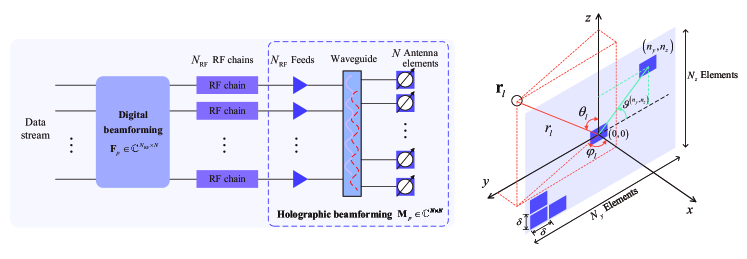
We consider an uplink holographic MIMO system where multiple single-antenna users are served by a base station (BS) having antenna elements in the form of a UPA. feeds are embedded in the substrate in order to generate reference waves carrying user-intended signals, with each feed connected to a radio frequency (RF) chain for signal processing. As illustrated in Fig. 1, the UPA coincides with the - plane and centered at the origin, where and denote the number of antenna elements along the - and -axis, respectively. For notational convenience, and are assumed to be odd numbers. The central location of the th antenna element is , in which and . Along the - and -axis, the physical measurements of the UPA are approximately and , respectively, with representing the inter-element spacing.
In contrast to the conventional array modeling that treats each antenna element as a sizeless point, the size of an antenna element, denoted by , should be explicitly addressed. It is possible to theoretically unify the modeling of continuous holographic surface and discrete antenna arrays by adjusting the element size and their inter-element spacing [17, 11], where . Particularly, let denote the array occupation ratio that indicates the portion of the entire UPA plate area being occupied by the antenna elements. Regarding the extreme case of , the UPA can be treated as a contiguous surface. Therefore, such a modeling is imperative to account for the projected aperture of each antenna element when signals are impinged from various directions, particularly in the presence of extremely large number of antenna elements. Furthermore, we assume in this paper that the effective antenna aperture is for the isotropic antenna element.
II-B Channel Model and Communication Protocol
We model the channel spanning from the BS to the user based on path parameters of the system [22, 26]. The assumption of the planar wavefront fails to describe the features of the link distance falling within the range of Rayleigh distance as EM waves do not uniformly radiate across different antenna elements. In this case, the generic spherical-wavefront model is essential to encapsulate phase variations across different antenna elements. In particular, we denote by the surface region of the th antenna element, and denote by the UPA normal vector, i.e., the unit vector along the direction. By taking into account the basic free-space propagations for a theoretical analysis, the channel power gain between the user and the th antenna element is given by [30]
| (1) |
where represents the distance between the user (or scatterer) and the reference antenna element of the UPA (i.e., ), and denotes the azimuth-elevation angle pair of the th path, with being the line-of-sight (LoS) path and being non-line-of-sight (NLoS) paths. The user location is determined by the LoS path, i.e., . The examination in (II-B) is applied to each individual antenna element, taking explicit account of the element size. More explicitly, the model in (II-B) accounts for the projected aperture of each antenna element, as reflected by the projection of the UPA normal vector to the wave propagation direction at each local point , in contrast to the conventional model for free-space path loss. In [31, 32, 33], similar models incorporating the projected aperture of the antenna element have also been considered for communicating with continuous surfaces. Hence, a two-dimensional integration over the surface of each element is required for a precise evaluation of (II-B).
Owing to the fact that each antenna element (not the entire array) in is on the wavelength scale, there may be typically marginal variations in the wave propagation distance and projection direction across different points . Hence, in light of the fact in [30], we have
| (2) |
which facilitates the approximation of the channel power gain in (II-B), i.e.,
| (3) |
Accordingly, the holographic channel between the BS and the user can be modeled as [22]
| (4) |
where denotes the channel coefficient of the th path and is the path number. Note that for the LoS path, i.e., , we denote , since the LoS path is distance-determinate [22, 9]. For the NLoS path, i.e., , the channel coefficient follows a complex Gaussian distribution, i.e., . The array response vector is structured by the following entry
| (5) |
where represents the extra-distance traveled by the wave to arrive at the th antenna element with respect to the reference one, and it can be unfolded as
|
|
(6) |
where herein represents the distance between the th antenna element and the reference one, and is a geometry term, with indicating the azimuth angle of the th antenna element with respect to the reference one.
For uplink channel estimation, it is assumed that the users transmit mutual orthogonal pilot sequences to the BS, e.g., by employing orthogonal frequency or time resources for different users, hence allowing the channel estimation to be independent of one another. Without loss of generality, we examine the channel estimation process of an arbitrary user. Denote by the pilot number and by user’s information-bearing signal, respectively, and the received signal at the BS is given by
| (7) |
where represents the combining matrix at the BS, is the holographic pattern that records the radiation amplitude of each antenna element, denotes the additive white Gaussian noise (AWGN) with power , and characterizes the channel spanning from the BS to the user. The aggregated received pilot sequence of all the uplink pilots from the user is given by
| (8) |
in which is the noise matrix, and delivers the overall observation matrix.
II-C Challenges
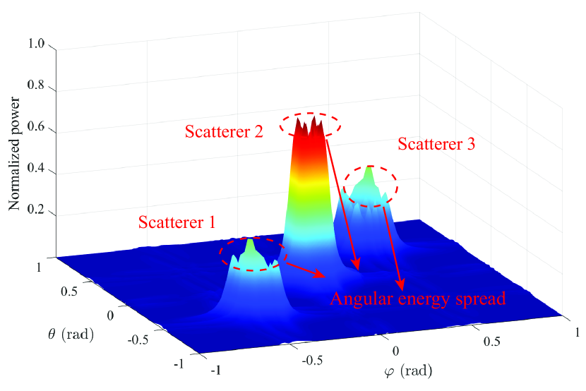
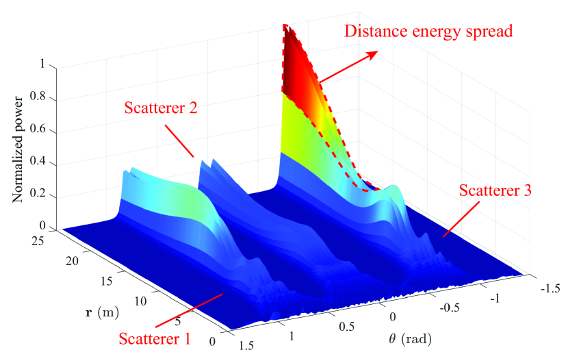
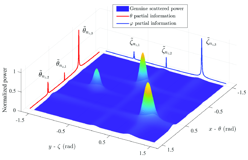
Most channel estimation schemes, being based on the classical planar-wavefront assumption, exploit the sparsity in the angular domain to achieve efficient estimation. However, this may result in severe energy spread effect in holographic MIMO counterparts. To be explicit, Fig. 2 portrays the power scattered in relation to the angle pair () in Fig. 2, and the power scattered in relation to the distance in Fig. 2, respectively, in which three scatterers are assumed in the propagation environment. As transpired in Fig. 2, the normalized power scattered typically results in the proliferation of angles, and fluctuates rapidly across the holographic antenna array. Despite the detachment of distance information , the true azimuth-elevation angle pair cannot be precisely distinguished. Additionally, as portrayed in Fig. 2, the power scattered versus the distance reveals a fluctuating trend from peak to trough. In this case, it is difficult to distinguish the genuine scattered power of the exact distance, since the energy may spread farther away with increased distance.
Actually, the angular-domain transform matrix just samples the angular information but ignores the distance information, which is implausible for the holographic near-field context due to the angles being functioned by the distance. Thus, the angular-domain transform matrix fails to align the sampling points to the genuine scattered power of the significant path corresponding to a user/scatterer. This always leads to a false alarm, i.e., the genuine channel power corresponding to the non-significant path is misinterpreted as a significant one, thus eroding the detection performance of the 3D AED parameters. To tackle this issue, we intend to achieve the effect decomposition of the 3D AED parameters by constructing their respective covariance matrices, for which each covariance matrix constructed retains its self-contained information while canceling out the potential impact of other parameters.
III Decomposition of 3D AED Parameters , , and
Given that the bare minimum of channel structure can be used when doing channel estimation, let us define as the matrix involving some appropriately selected entries from the covariance matrix of the exact channel, whose th entry can be given by
| (9) | ||||
where and holds owing to the orthogonal assumption between two independent paths. Although represents a part of the covariance matrix, we refer to it as the covariance matrix throughout of this paper. As observed in (III), is dependent on the distance difference with respect to the antenna elements and . Using the Fresnel approximation [34], (6) can be further recast to
| (10) |
in which the first term involves both the angular and distance information, while the second term pertains exclusively to the angular information, i.e., . This property is paramount since it inspires the subsequent parametric deconstruction. In the subsections that follows, tailored tricks are presented for effectively decomposing the tightly coupled 3D AED parameters.
III-A Angular Decomposition
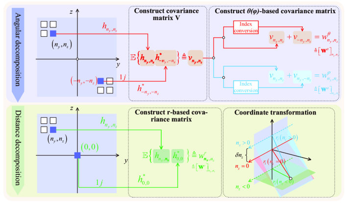
The structure of (10) inspires a potential technique to select the index of the th entry of the conjugate channel with extra care for ensuring that is determined exclusively by the angular information. The index selection strategy needs to satisfy and . This pair of restrictions can be readily addressed by letting , and thus in (III) can be trimmed to
| (11) |
The physical significance behind this index selection trick is to allow the indices of the antenna elements corresponding to the channel and its conjugate copy to be symmetrical to the origin, as illustrated in Fig. 3. As a result, retains only the angular information of the original channel structure. To facilitate the reduced searching space in the estimation process, the decomposition can be further refined to trim the 2D model at hand into a pair of 1D quantities consisting exclusively of or .
III-A1 Extraction of
We aim to retain the -associated term in the phase of , i.e., , by constructing a -based covariance matrix . Particularly, the th entry in can be calculated by . By letting , we have
| (12) |
We let the antenna element spacing be , and the th entry of the -based covariance matrix takes the form of
| (13) |
Note that conveys double implications, that is, it not only indicates a denser antenna spacing in the holographic MIMO of interest, but it also complies with the Nyquist sampling theorem under the DeRe framework for acquiring statistical characteristics of (i.e., -based covariance matrix ). To be explicit, it is evident from (III-A1) that the estimation of is equivalent to identifying all spectral power peaks with the frequency index given the sequences with the time index . The phase term in (III-A1), i.e., , can be structured as a standard Fourier-like form, namely . The frequency component has to follows Nyquist sampling theorem, yielding that , and we thus have . Additionally, as for the constructed -based covariance matrix , the row vectors thereof, i.e., , are independent of one another. Each independent vector delivers an observation indexed by for the estimate of , i.e., , in which these estimates contribute in collaboration to a faithful , as elaborated on later.
III-A2 Extraction of
The same technique can be applied to construct the -based covariance matrix , but using a different index-selection strategy, i.e., , hence yielding
| (14) |
As shown in (III-A2), both the amplitude and phase of contains the information of , which implies that an estimate of is a prerequisite for the determination of . The -based covariance matrix incorporates independent vectors with vector size . In other words, the th column vector of serves as an observation that can be used for the CS process to attain , the estimates of which can be appropriately fused by a sophisticated design for the robust recovery of . Further details appear in Sec. V.
III-B Distance Decomposition
The distance decomposition can be achieved by constructing the -based covariance matrix that strips out the angular information for retrieving the distance information. Specifically, we use the same trick when constructing . As illustrated in Fig. 3, we employ the channel and its conjugate copy corresponding to the origin of the UPA, namely , as a pair of inputs for , i.e.,
| (15) |
Recall that the distance difference takes the form of , with . By substituting them into (III-B), we have (16) presented at the top of the next page.
| (16) |
For simplicity, we firstly consider a special case of , and hence (16) can be trimmed to (17), shown at the top of the next page.
| (17) |
A closed examination in (17) indicates that the recovery of the distance from relies upon the acquisition of the azimuth-elevation angle pair , which has a direct impact on the algorithm flow, as will be detailed in Sec. V. Additionally, for a more general instance of , the same form as (17) can be attained by shifting the reference system by (m) along the -axis using the coordinate transformation.
Thus far, we have achieved the decomposition of the 3D AED parameters by constructing their associated covariance matrices, each of which retains fully knowledge that can be explored. In light of the closed structures in (13), (III-A2) and (17), we are inspired to conduct the CS procedure on each parameter to ensure their accurate and robust recoveries. Therefore, the following of this treatise moves on to describe in great detail the CS-based reconstruction, along with an efficient algorithm proposed for resolving CS-related setbacks.
IV CS-based Reconstruction
IV-A CS Formulation of
The constructed -based covariance matrix encompasses vectors with vector size , in which the th vector can be drawn out from given by . The vector is actually an observation interpreted as a linear combination of all steering vectors shown in (13). Furthermore, a wide measurement matrix can be introduced for a lower-dimension observation , thus yielding
| (18) |
where the entries in are allowed to follow a complex Gaussian distribution .
Given that there are only significant angles of arrival (AoAs) in the physical propagation environment, it is beneficial to mine the sparse characteristics concealed behind for achieving sparse estimates of AoAs at reduced complexity and overhead. For this purpose, a uniform grid of AoAs over are prescribed to take values from the discrete sets . Nevertheless, the true AoAs do not coincide exactly with the grid points. To capture the attributes of mismatches between the true angles and the grid points, the off-grid basis is harnessed for its sparse representation [35]. More precisely, we introduce the -based offset vector , in which is given by
| (19) |
in which indicates the index of the AoA grid point nearest to the AoA of the th path. Thus, can be structured as
| (20) |
where is an -sparse vector, is the noise vector, and is the dictionary matrix. The design of the dictionary matrix is required to satisfy the RIP condition in order to facilitate the accurate sparse signal recovery. As a necessity for accurate sparse signal recovery, the dictionary matrix has to satisfy the RIP condition [35] for eliminating the grid coherence, which adversely impacts the estimation performance. To be specific, the RIP condition can be interpreted as two arbitrary columns being (approximately) orthogonal, where the th entry of is crafted by . Thus, (18) can be recast to a CS form with uncertain dictionary matrix (containing the to-be-determined ) and sparse vector , i.e.,
| (21) |
IV-B CS Formulation of
The CS reconstruction for can be executed using similar tactics to those employed in ’s. However, the phase term in (III-A2) includes the -associated part, which may preclude the direct gridding over . To resolve this hiccup, we introduce an intermediate variable for satisfying . Next, an arbitrary vector indexed by can be extracted from the -based covariance matrix , i.e., . A wide measurement matrix is left-multiplied by the vector for confining its size with the number of RF chains, thus yielding . To perform gridding over , a uniform grid of angles is introduced, i.e., . Regarding the mismatches between the true angles and the prescribed grid points, -based offset vector is defined as , with given by
| (22) |
in which indicates the index of the AoA grid point nearest to the AoA of the th path. Thus, can be structured as a CS form
| (23) |
in which is an -sparse vector, is the noise vector, and represents the dictionary matrix, whose th entry is given by . Therefore, the -based observation can be recast to
| (24) |
IV-C CS Formulation of
An arbitrary vector indexed by can be drawn out from the -based covariance matrix , i.e., . To facilitate the gridding over distance, we likewise introduce a uniform grid of discrete points of , i.e.,
| (25) |
where is the minimum value to ensure the approximate orthogonality of the dictionary matrix with representing the orthogonality controlling factor in order to make sure the grid coherence being below [26]. Taking into account the upper and lower bounds of the Rayleigh distance, i.e., ( is the array aperture), the number of the grid points can be determined in accordance with (), and the maximum of takes the value of
| (26) |
Furthermore, the -based offset vector is specified with its th entry given by
| (27) |
where indicates the index of the distance grid point nearest to the distance of the th path. Then, denoting and by the -based observation vector and the sparse vector, respectively, we can likewise structure as its CS form
| (28) |
where is the size-reducing measurement matrix, is the noise vector, and , is the dictionary matrix, whose th entry is given by
| (29) |
IV-D Discussion
Our goal is to obtain the offset vectors , and from the 3D AED parameter-based CS problem given in (21), (24), and (28), respectively. Then, the 3D AED parameter can be recovered by , , and . The way to accurately acquire the offset vectors will be elaborated in the next section. Let us look first at a pair of two issues, in which how the proposed DeRe paradigm is a curse when concerned in terms of angular index misinterpretations but a blessing when embraced with regard to significantly reduced gridding complexity.
IV-D1 Angular Index Correction
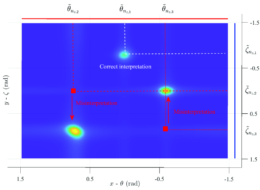
The outputs of the DeRe framework, i.e., , , and , just play separate roles on a significant path, which can be referred to as the partial information. When recovering the original holographic channel using the obtained independent partial information, there typically exist the angular index misinterpretations which significantly deteriorate the estimation performance. To elaborate, in examination of case , Fig. 4 portrays the genuine angular power scattered in relation to the azimuth-elevation angle pair after DeRe filtering, as well as the misinterpretation between the attained angular indices and the true indices of the significant angles when used with partial information. There exist three zero-entries in each of the sparse vectors and . By retrieving the indices of the non-zero entries for this pair of sparse vectors, the true index of the th significant angle pair may be adversely misinterpreted for that of other significant angle pairs. For example, having retrieved the index for and , we may obtain a significant angle pair and (with red marker in Fig. 4). However, this results in a false index for the genuine significant angle pair associated with the path whose true index is . Such a misinterpretation significantly erodes the estimation accuracy. To address this hiccup, it is crucial to conduct the angular index correction after attaining the estimates of and .
Regarding the th entry in the -based sparse vector , we denote by its index of the non-zero entry, whose th non-zero entry is given by
| (30) |
Similarly, the non-zero entry in the -based sparse vector indexed by is given by
| (31) |
Since there are paths in total, there will be misinterpretation combinations. We are trying to identify the true indices of the azimuth and elevation angles associated with the th path. To this end, a pair of variables and are introduced to represent the power gain of the th path (i.e., ) associated with the decomposed and , respectively. Given and , we have
| (32) | ||||
| (33) |
The idea of the angular index correction is straightforward, that is, identifying the two entries with the closest power, and matching their indices to the index of the path. Therefore, we can accurately retrieve the exact index of the th path associated with the azimuth-elevation angle pair ()
| (34) |
Having identified the true index , the power gain can be obtained by .
IV-D2 Gridding Complexity
The use of the DeRe framework is capable of significantly reducing the gridding complexity. In particular, gridding across the coupled 3D AED parameters has a complexity order of , in conjunction with . Consequently, the estimation process would be less efficient owing to the resultant extremely large search space. By contrast, 1D gridding over has a complexity order of , and gridding over both and shares the same complexity order of , which leads to a total gridding complexity order of . Therefore, it is intuitive that the original multiplicative gridding complexity is relaxed to its additive counterpart, significantly lowering the computational burden in practice.
IV-E Robustness of DeRe Framework
Given the potential adverse effects of hardware imperfections, such as deviations between the practical and theoretical designs of the combining matrix and holographic pattern , this subsection aims for examining the robustness of the DeRe framework against such perturbations in the context of channel estimation. Note that is actually a fictitious vector for ease of analysis (as are and ), so before proceeding to unveiling DeRe’s robustness, let us establish a critical bridge between the physical signal received from the BS and the observation utilized in the CS procedure. Subsequently, we shall take as an illustrative instance.
Let denote an arbitrary sample of the received signal at the BS. We define as the mapping from to . For an arbitrary observation sampled at , we obtain , whose mapping relation is given by . The mapping can be recast by means of a matrix manipulation given by
| (35) |
where , with the th vector given by and representing the basis vector whose th entry is non-zero. The matrix is constituted by , whose th vector is crafted by
| (36) |
It thus holds that , in which the implementation of is similar to ’s, just using different index selection strategy shown in (III). As a result, the received signal at the BS that serves as an observation can be given by
| (37) |
In practical systems, the linear transformation in (IV-E), i.e., can be achieved by appropriately designing the combining matrix and the holographic pattern. The remnant expectation term can be realized by an output of the Hadamard product whose inputs take the signal received at the BS and its conjugate counterpart.
The structure in (IV-E) indicates that the signal received at the BS can be crafted to attain the observation embracing -associated statistical characteristics. Regarding the error induced by hardware imperfections, we let , where denote the intended design of the combining matrix and holographic pattern, while captures the deviation between the actual implementation and the intended design. Accordingly, (IV-E) can be recast as
| (38) |
The form in (IV-E) is appealing since it is analytically tractable. This implies that the resultant error can be mitigated through skillful designs of the combining matrix and holographic pattern. Specific design details are beyond the scope of this paper, and interested readers may refer to [36, 37] for inspiration in transceiver design within the context of holographic scope. The robustness performance of the DeRe framework will be evaluated later in Sec. VI.
V DeRe-VM Algorithm
In pursuit of an accurate and robust channel estimation for holographic MIMO systems, we intend to recover the sparse vectors , and , as well as their associated offset vectors , and , as presented in (21), (24), and (28), respectively. Albeit the seeming straightforwardness of that kind of parameter-recovery problem, it poses arduous challenges due to a pair of peculiarities: i) the uncertainty of the sensing matrices including the offsets to be determined, i.e., , , and , as well as ii) the imperfect priors of the sparse vectors induced by the unavailability of the exact distributions for , , and . Therefore, targeting the twofold issues, a layered probability model is leveraged to provide appropriate prior distributions for the sparse vectors, followed by an efficient and robust algorithm design.
V-A Layered Probability Model
For the sake of brevity, we take as an example to explicate the way to harness the structured sparsity underlying . Concerning that estimates of can be attained by resolving copies of problem (21), we can group the sparse vectors into blocks with block size , in which the th block is given by . Let represent the precision vector, in which denotes the variance of . Furthermore, a support vector denoted by is introduced, whose th entry indicates whether the th block is active () or not (). Therefore, the joint distribution of , , and is in the form of
| (39) |
Then let us move on to describe in greater detail the prior distribution of each layer.
V-A1 Layer I: Probability Model for Support Vector
Due to the limited scatterers in the physical propagation environment, the birth-death process of can be modeled as a Markov prior
| (40) |
with the transition probability given by
| (41) |
where represents the transition probability of entries in the sparse vector shifting from 0 to 1, and vice versa for .
V-A2 Layer II: Probability Model for Precision Vector
A Gamma prior distribution is imposed on the precision vector of the support vector
| (42) |
where is a Gamma hyperprior with the shape parameter and rate parameter . For the case of , the shape and rate parameters and are selected to satisfy , since the variance of is equivalent to and deviates from zero with a high probability when it is active. On the contrary, we let the shape and rate parameters and be chosen such that , conditioned on the event of , in which case the variance of tends to be zero when the associated path is inactive.
V-A3 Layer III: Probability Model for Sparse Vector
The conditional probability for sparse vector is considered to follow a non-stationary Gaussian prior distribution with distinct precision
| (43) |
Additionally, in the presence of the complex Gaussian noise, we have
| (44) |
where represents the noise precision that follows a Gamma hyperprior . The tunable and tend to zero, i.e., , for approximating a more general hyperprior.
V-A4 Channel Recovery Problem Formulation
Given observations , our objective is to estimate the sparse vector and the grid offsets . More precisely, we intend to compute the MMSE estimates of , i.e., , with the expectation taken over the conditional marginal posterior
| (45) |
where represents the entry removal with respect to over the sparse vector and refers to the equality after scaling. Furthermore, the uncertain grid offset can be attained by MLE as
| (46) |
in which represents the collection of variables associated with the probability model. We thus attain the MMSE estimate of by figuring out the MLE of and the conditional marginal posterior .
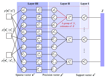
Recall that estimates of can be attained by solving copies of problem (21), and the associated sparse vectors have been grouped into blocks with block size , as illustrated in the factor graph in Fig. 5. Such a grouping facilitates an appropriate fusion of beliefs, i.e., messages passing via the path . To be explicit, in light of the belief propagation [38], the message is calculated by taking the product of all messages received by the factor node on all other edges, i.e.,
| (47) |
This implies that each block contains partial priors of the sparse vectors, and priors of blocks function collaboratively on the channel support vector .
It is still arduous to obtain the precise estimates of and , since the conditional marginal posterior in (V-A4) is unavailable due to the complex integration, and the dense loops in the factor graph exacerbate matters. Additionally, the non-concave nature of problem (46) hinders the pursuit of its stationary solution even if one uses some plain optimization approaches. Therefore, the subsection that follows proceeds to present beneficial techniques for clearing up the above hindrances, as well as an effective algorithm for facilitating the efficient estimation of .
V-B DeRe-VM Algorithm
As a key feature of DeRe-VM, an approximate variational distribution is employed to refine the intractable posterior in the DeRe-VM-E Step, while updating the indeterminate grid offset using the gradient-based technique in the DeRe-VM-M Step.
V-B1 DeRe-VM-M Step: Inexact Majorization-Minimization (MM)
The likelihood function
is indeed intractable owing to the absence of closed-form expressions induced by the prohibitive integrals of the joint distribution with regard to indeterminate . An alternative is to construct its surrogate function based on in the th iteration in place of the objective in problem (46), providing that the exact posterior has been identified. Unfortunately, the exact posterior is also highly unavailable in our examined problem owing to the intricate loops inherent in the factor graph. We thus need to leverage the variational Bayesian inference (VBI) and message passing techniques to attain an alternative for a faithful approximation of the conditional posterior . The to-be-determined posterior has a factorized form, i.e., , with representing an individual in the variable collection , and we have . Then, an equivalent of the original MLE problem in (46) can be obtained based on the approximate posterior, which is formulated as
| (48) |
In the th iteration in the DeRe-VM-M Step, can be updated by
| (49) |
The non-concave nature of the objective, nevertheless, impedes the pursuit of the global optimum for problem (49). We thus exploit the following gradient update in an effort to obtain a stationary solution
| (50) |
where is the step size determined by the Armijo rule [35].
V-B2 DeRe-VM-E Step: A Pair of Entities
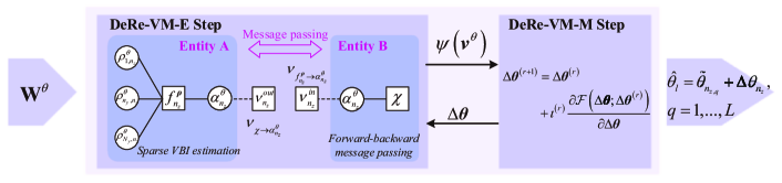
Due to myriads of loops in a dense factor graph depicted in Fig. 5, a direct employment of the classical sum-product message passing (SPMP) [39] fails to traverse the factor and variable nodes over the entire factor graph. As potential solutions, the approximate message passing (AMP)-based algorithms, e.g., Turbo-AMP [40] and Turbo-CS [41], easily get entrapped into their poor local optimum due to the ill-conditioned dictionary matrix induced by the indeterminate . To facilitate the practical implementation, two entities are specified in the DeRe-VM-E Step, namely Entity A and Entity B as exemplified in Fig. 6, in support of the sparse VBI estimates and forward-backward message passing. Furthermore, this pair of entities need to interact with each other to eliminate the self-reinforcement during the update procedure.
-
•
Entity A: By capitalizing sparse VBI [42], this entity intends to calculate the approximate conditional marginal posteriors of latent variables, i.e., . We denote by the input of Entity A, which is actually the message passed from Entity B and incorporates the Markov priors of the structured sparsity associated with the sparse vector . The sparse VBI estimates implemented in Entity A will be elaborated on later.
-
•
Entity B: Let denote the message passed from Entity A, which constitutes the input of Entity B. To facilitate exposition, the input and the output of Entity B are defined as and , respectively. In each algorithm iteration, the message can be obtained in accordance with the belief propagation rule [39, 38]
(51) which intuitively equals the approximate posterior with respect to , since plays the role of Entity A’s prior with respect to . The inference also holds for Entity B’s output, and this pair of entities would interact iteratively until their convergence has been achieved.
Having established the method for carrying out message exchange between the twin entities, let us move on to an elaboration of the sparse VBI estimation in Entity A for closed-form updates of the associated posteriors.
V-B3 Entity A: Sparse VBI Estimation
Firstly, to determine the approximate conditional marginal posterior , the sparse VBI estimation can be outlined as a minimization of the Kullback-Leibler divergence (KLD) with respect to and , thus yielding that
| (52a) | ||||
| (52b) | ||||
The stationary point to problem (52a) needs to satisfy
| (53) |
which can be attained via alternating updates of . Specifically, for given , the optimal that satisfies the KLD minimization in problem (52a) is specified as
| (54) |
where .
Secondly, the posteriors , and can be updated as follows.
-
•
Update sparse vector : can be updated by a complex Gaussian distribution
(55) and can be calculated by
(56) (57) where , , and .
-
•
Update precision vector : is given by
(58) where , , and represents the posterior probability of , also known as the message passed from Entity A.
-
•
Update support vector : We obtain the posterior in the form of
(59)
Likewise, the foregoing procedures are also applicable to both and for obtaining their CS-based solutions. When establishing the layered processing probability model and conducting sparse estimation techniques, we just use and in place of the superscript of associated variables, e.g., and , etc., and the corresponding phases have been omitted for conciseness. In brief, the proposed DeRe-VM algorithm have been summarized in Algorithm 1.
V-C Computational Complexity
Following the overall flow of DDS-VBIMP summarized in Algorithm 1, the main computational burden lies in the updates of , , and in Step 9 using (55)-(59), respectively. The total number of multiplications to update is . Upon the utilization of the matrix inversion lemma on (56) in order to lower complexity, the computational complexity with regard to the matrix inversion in (56) is . Thus, the total computational complexity order of the proposed DeRe-VM algorithm is per iteration, concerning that it typically holds that . This implies that for an -element UPA (), the complexity of the proposed DeRe-VM algorithm just scales proportionally with the number of antenna elements raised to the power of 1.5. Additionally, our proposed DeRe-VM algorithm functions within the off-grid basis and is capable of eliminating on-grid errors, sharing the similarities with the methodology presented in [26], namely polar-domain simultaneous gridless weighted (P-SIGW). Albeit the evident superiority of P-SIGW, there are two issues that should be taken with a grain of salt: i) P-SIGW fails to capture the coherence between the 2D elevation-azimuth angle pair and the distance for a robust recovery of 3D AED parameters, and ii) the computational complexity of P-SIGW increases quadratically with the number of antenna elements, making it less favorable for a large . In the section that follows, a comprehensive performance evaluation will be illustrated, showcasing their distinct advantages in relation to various cases.
VI Simulation Results
VI-A Configuration
In this section, we conduct performance evaluation of the proposed DeRe-VM algorithm for channel estimation in the holographic MIMO system of interest. The antenna elements at the BS are equipped in the form of and . The considered holographic MIMO system operates at 30 GHz with a bandwidth of 100 MHz. It is assumed that the number of paths is . The simulation results are averaged over 500 random channel realizations. For each realization, the distance between the BS and the user/scatterer is sampled from a uniform distribution , and based on the fixed distance, the associated angular parameters of the LoS path are randomly sampled from the uniform distributions and , respectively. Furthermore, the complex gain of each NLoS path is modeled to follow a complex Gaussian distribution with zero mean and variance , i.e., , in which is 20 dBm weaker than that of the LoS paths [43]. In the process of the CS reconstruction, the number of the uniform grid is set to for , and for , respectively. We concentrate on the normalized mean square error (NMSE) performance of the auto-correlation matrix , which can be reconstructed by after we obtain the estimates of the 3D AED parameters , , and . The NMSE is defined as . Other key system parameters are set as follows unless otherwise specified: , , dBm, , , , , .
VI-B Convergence Behavior
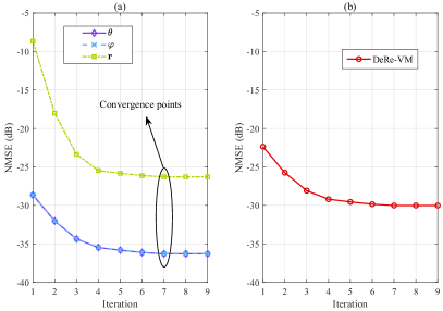
We demonstrate the convergence behavior of the proposed DeRe-VM algorithm by plotting the NMSE curves of 3D AED parameters , , and in Fig. 7(a), which is calculated by [44]. By contrast, Fig. 7(b) shows the NMSE performance of the auto-correlation matrix, obtained by . A steep decline can be spotted in the first few iterations, followed by a gradual settling at a value after around seven iterations for both scenarios. The NMSE gap in accuracy between and can be attributed to the presence of a residual correlation inside the distance dictionary matrix. Albeit this non-orthogonality, DeRe-VM still exhibits favorable estimation precision in terms of ’s NMSE performance.
VI-C NMSE Performance
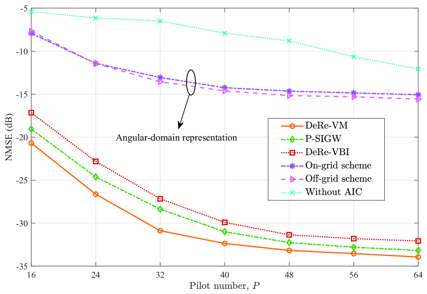
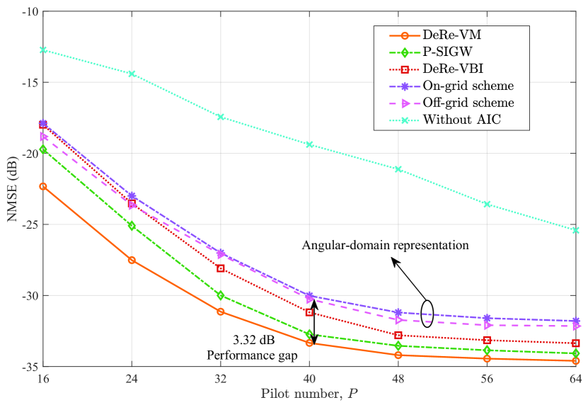
For comparison, the exploited benchmark schemes are listed as follows:
-
•
P-SIGW [26]: The off-grid polar-domain simultaneous iterative gridless weighted (P-SIGW) algorithm exploits different transform matrix constructed for the independent decomposition of angle and distance parameters.
- •
-
•
Off-grid scheme [35]: The holographic MIMO channel is treated in the angular domain using VBI approach.
- •
-
•
Without AIC: The angular index correction in Step 20 of Algorithm 1 is removed.
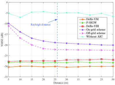
We begin the NMSE performance evaluation by investigating their corresponding curves versus the BS-to-user distance ranging from 5 m to 50 m. In accordance with the carrier frequency of 30 GHz and the number of antenna elements of and , the Rayleigh distance can be determined to be 26 meters. As shown in Fig. 8, the proposed DeRe-VM algorithm consistently reveals the best NMSE performance, whereas that of the scheme Without AIC swings erratically as the distance increases from the near-field to the far-field. The poor NMSE performance attained by the scheme Without AIC results from the ambiguity of imposed by the thoughtlessly stitching of the 3D AED parameters, as the angular index misinterpretation frequently occurs. Furthermore, a NMSE performance leveling off is spotted with respect to the schemes incorporating distance estimation, e.g., DeRe-VM, P-SIGW, and DeRe-VBI, regardless of fluctuations in distance. In contrast, both on-grid and off-grid schemes exhibit poor estimating performance, particularly in the near-field region. This is primarily due to the fact that distance-estimation schemes are capable of structuring distance grids in a sense that accommodates to various channel environments. More precisely, when doing gridding over the distance , a uniform grid of discrete points embraces the far-field case, i.e., in (25), allowing the far-field information to be retrieved from the -based covariance matrix. Therefore, the proposed DeRe-VM reveals significant robustness in accommodating diverse channel conditions at varying distances in the context of a holographic MIMO system.
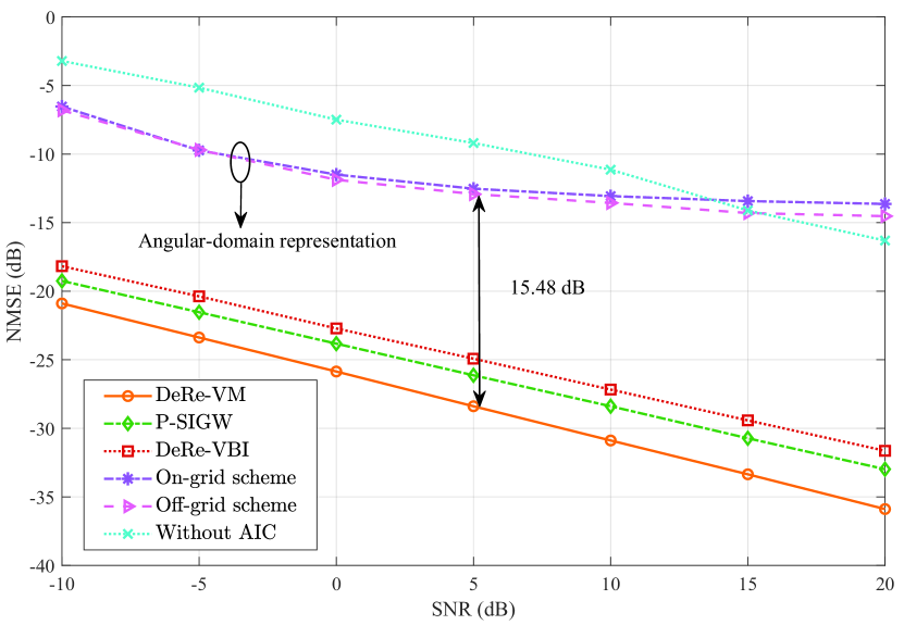
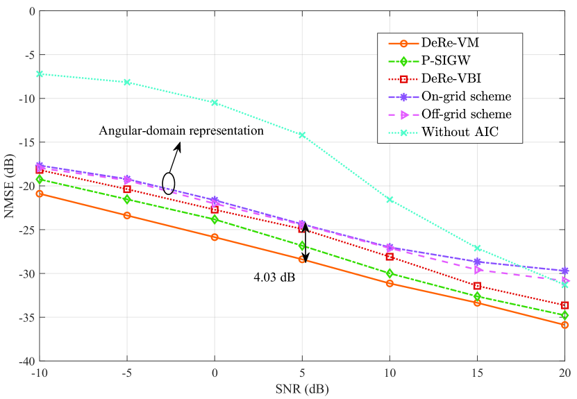
In Fig. 9, we investigate the impact of varying SNR on the NMSE performance for different BS-to-user distance configurations, where the 26-meter Rayleigh distance is taken as the dividing line for the near-field and far-field regions. Firstly, as expected, an increase in SNR boosts the NMSE performance and the proposed DeRe-VM algorithm is superior to the benchmark schemes adopted, regardless of the distance configurations. This is made possible by the fact that DeRe-VM offers the capability of capturing, via their independent decompositions, potential structured sparsities in relation to 3D AED parameters in holographic MIMO channels. On the other hand, the scatterers in the physical environment can be characterized by Markov prior for the channel support , which also explains the reason why DeRe-VM is superior to DeRe-VBI. Secondly, the NMSE performance achieved by on-grid and off-grid schemes significantly enhances when the examined settings shift to the far-field case. For instance, as SNR = 5 dB, the performance gap resulted from DeRe-VM and off-grid schemes falls from 15.48 dB in the near-field case to 4.03 dB in the far-field case. Additionally, one interesting finding is that in the far-field configuration, higher SNR draws the NMSE performance achieved by Without AIC to a great level, in stark contrast to the pale efforts made by the increased SNR for the marginal improvement of NMSE in the near-field context. This is because a high SNR can compensate for the erroneous estimation caused by the absence of the angular index correction when just estimating the 2D azimuth-elevation angle pair.
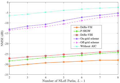
Fig. 10 plots the NMSE curves in relation to the pilot length for various distance cases, as in Fig. 9. With more pilots inserted, holographic MIMO channels can be better characterized, resulting in a diffing degree of improvement for NMSE with various schemes. To be specific, regarding showcased in Fig. 10, an increment in boost NMSE performance marginally in the near-field case while considerably in the far-field case. This can be attributed to the fact that on- and off-grid schemes based on the angular-domain representation suffer from a performance bottleneck induced by a severe energy spread and erroneous detection of significant paths. Interestingly, both cases demonstrate a slight decline in NMSE when , in contrast to a precipitous drop when , which implies a potential compromise between the pilot number and NMSE, that is, favorable NMSE performance can be achieved given an appropriate , while a large may incur heavy pilot overhead for systems. Additionally, the performance gap can still be spotted in Fig. 10, e.g., 3.32 dB when , between DeRe-VM and On-grid schemes, owing to a more accurate Fresnel approximation in (10) than its far-field counterpart.
Fig. 11 demonstrates the variation of NMSE performance with respect to the number of NLoS paths among different schemes. Since represents the LoS path, the number of NLoS paths is denoted by . As spotted in Fig. 11, the NMSE performance achieved by all the schemes being considered exhibits a slight degradation with an increased number of NLoS paths, albeit to different degrees. As the number of NLoS paths increases, an augmentation occurs in the quantity of non-zero entries within each sparse vector. This without a doubt increases the dimensionality of the solution space, rendering the CS-based algorithm more susceptible to becoming ensnared in local optima in the pursuit of the optimal value. As a result, figuring out the LoS path becomes more challenging. Fortunately, due to the “turbo” nature of DeRe-VM, with which the updates of parameters and posteriors mutually reinforce each other, it can be ensured that the algorithm will eventually converge to a stationary point [46, 47].
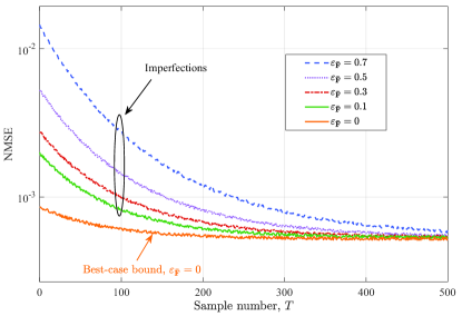
To evaluate the robustness of the proposed DeRe framework, Fig. 12 plots the NMSE curves versus the sample number . In conjunction with (IV-E), we define as the error ratio to quantify the level of hardware imperfections induced by for example, the limited resolution of phase shifters and amplitude controllers. As it transpires, the NMSE performance is expected to improve with an increase in the number of samples. An eye-catching observation pertains to the existence of gaps in NMSE performances across various in the presence of a small number of training samples, while the NMSE performance achieved by all cases, as grows larger, tends to approach the best-case bound. This verifies that the DeRe framework has the capability to learn the statistical properties of the 3D AED parameters by harnessing the samples adequately despite the presence of hardware imperfections, showcasing the great robustness of the proposed DeRe framework.
VII Conclusion
In this work, we have investigated the channel estimation for holographic MIMO systems in face of a few non-trivial challenges posed by the holographic MIMO nature. A sophisticated DeRe framework is devised for deep decouplings of the 3D AED parameters, followed by an efficient DeRe-VM algorithm for resolving the resultant CS problems. We evince that the implementation of the proposed DeRe framework facilitates sharp detection of the parameters for each dimension, but it may adversely results in misinterpretation of the angular index if these quantities obtained are not properly structured together. As a remedy, angular index correction is carried out for the accurate estimation. Our simulation results substantiate that the proposed DeRe-VM algorithm exhibits great robustness to the distance fluctuations in the holographic MIMO system of interest, irrespective of whether the scenario involves near-field or far-field. In contrast to the conventional far-field solutions based on the angular domain, the proposed DeRe-VM paradigm still shows slightly improved NMSE performance owing to its employment of a more accurate Fresnel approximation, without noticeable increase in sparsifying complexity.
References
- [1] C.-X. Wang et al., “On the road to 6G: Visions, requirements, key technologies, and testbeds,” IEEE Commun. Surv. Tutor., vol. 25, no. 2, pp. 905–974, Second-quarter, 2023.
- [2] J. M. Jornet, E. W. Knightly, and D. M. Mittleman, “Wireless communications sensing and security above 100 GHz,” Nat. Commun., vol. 14, no. 1, p. 841, Feb. 2023.
- [3] M. Matthaiou, O. Yurduseven, H. Q. Ngo, D. Morales-Jimenez, S. L. Cotton, and V. F. Fusco, “The road to 6G: Ten physical layer challenges for communications engineers,” IEEE Commun. Mag., vol. 59, no. 1, pp. 64–69, Jan. 2021.
- [4] “Technical specification group services and system aspects; Release 17 description; summary of Rel-17 work items,” 3rd Generation Partnership Project, Tech. Rep. 3GPP TR 21.917 V0.7.0, Jun. 2022.
- [5] A. R. Flores and R. C. de Lamare, “Robust and adaptive power allocation techniques for rate splitting based MU-MIMO systems,” IEEE Trans. Commun., vol. 70, no. 7, pp. 4656–4670, Jul. 2022.
- [6] A. M. Elbir, K. V. Mishra, M. R. B. Shankar, and S. Chatzinotas, “The rise of intelligent reflecting surfaces in integrated sensing and communications paradigms,” IEEE Netw., to appear, 2022.
- [7] C.-Y. Yeh and E. W. Knightly, “Eavesdropping in massive MIMO: New vulnerabilities and countermeasures,” IEEE Trans. Wireless Commun., vol. 20, no. 10, pp. 6536–6550, Oct. 2021.
- [8] E. Shtaiwi, H. Zhang, S. Vishwanath, M. Youssef, A. Abdelhadi, and Z. Han, “Channel estimation approach for RIS assisted MIMO systems,” IEEE Trans. on Cogn. Commun. Netw., vol. 7, no. 2, pp. 452–465, Jun. 2021.
- [9] Y. Chen, Y. Wang, Z. Wang, and P. Zhang, “Robust beamforming for active reconfigurable intelligent omni-surface in vehicular communications,” IEEE J. Sel. Areas Commun., vol. 40, no. 10, pp. 3086–3103, Oct. 2022.
- [10] G. Kramer, “Information rates for channels with fading, side information and adaptive codewords,” arXiv preprint: 2302.02903, 2023.
- [11] C. Huang, S. Hu, G. C. Alexandropoulos, A. Zappone, C. Yuen, R. Zhang, M. D. Renzo, and M. Debbah, “Holographic MIMO surfaces for 6G wireless networks: Opportunities, challenges, and trends,” IEEE Wireless Commun., vol. 27, no. 5, pp. 118–125, Oct. 2020.
- [12] R. Deng, B. Di, H. Zhang, D. Niyato, Z. Han, H. V. Poor, and L. Song, “Reconfigurable holographic surfaces for future wireless communications,” IEEE Wireless Commun., vol. 28, no. 6, pp. 126–131, Dec. 2021.
- [13] T. Gong, P. Gavriilidis, R. Ji, C. Huang, G. C. Alexandropoulos, L. Wei, Z. Zhang, M. Debbah, H. V. Poor, and C. Yuen, “Holographic MIMO communications: Theoretical foundations, enabling technologies, and future directions,” IEEE Commun. Surv. Tutor., to appear, 2023.
- [14] A. A. D’Amico and L. Sanguinetti, “Holographic MIMO communications: What is the benefit of closely spaced antennas?” arXiv preprint: 2307.13467, 2023.
- [15] T. L. Marzetta, “Super-directive antenna arrays: Fundamentals and new perspectives,” in 2019 53th Asilomar Conf. Signals, Sys., Comp., Pacific Grove, CA, USA, Nov. 2019, pp. 1–4.
- [16] L. Han, H. Yin, M. Gao, and J. Xie, “A superdirective beamforming approach with impedance coupling and field coupling for compact antenna arrays,” arXiv preprint: 2302.08203, 2023.
- [17] A. Pizzo, L. Sanguinetti, and T. L. Marzetta, “Fourier plane-wave series expansion for holographic MIMO communications,” IEEE Trans. Wireless Commun., vol. 21, no. 9, pp. 6890–6905, Sep. 2022.
- [18] A. Pizzo, T. L. Marzetta, and L. Sanguinetti, “Spatially-stationary model for holographic mimo small-scale fading,” IEEE J. Sel. Areas Commun., vol. 38, no. 9, pp. 1964–1979, Sep. 2020.
- [19] Ö. T. Demir, E. Björnson, and L. Sanguinetti, “Channel modeling and channel estimation for holographic massive MIMO with planar arrays,” IEEE Wireless Commun. Lett., vol. 11, no. 5, pp. 997–1001, May 2022.
- [20] L. Wei et al., “Multi-user holographic MIMO surfaces: Channel modeling and spectral efficiency analysis,” IEEE J. Sel. Topics Signal Process., vol. 16, no. 5, pp. 1112–1124, Aug. 2022.
- [21] L. Wei, C. Huang, G. C. Alexandropoulos, Z. Yang, J. Yang, W. E. I. Sha, Z. Zhang, M. Debbah, and C. Yuen, “Tri-polarized holographic MIMO surfaces for near-field communications: Channel modeling and precoding design,” IEEE Trans. Wireless Commun., to appear, 2023.
- [22] M. Ghermezcheshmeh, V. Jamali, H. Gacanin, and N. Zlatanov, “Parametric channel estimation for LoS dominated holographic massive MIMO systems,” arXiv preprint: 2112.02874, 2022.
- [23] R. Deng, B. Di, H. Zhang, and L. Song, “HDMA: Holographic-pattern division multiple access,” IEEE J. Sel. Areas Commun., vol. 40, no. 4, pp. 1317–1332, Apr. 2022.
- [24] R. Deng, B. Di, H. Zhang, Y. Tan, and L. Song, “Reconfigurable holographic surface-enabled multi-user wireless communications: Amplitude-controlled holographic beamforming,” IEEE Trans. Wireless Commun., vol. 21, no. 8, pp. 6003–6017, Aug. 2022.
- [25] H. Zhang, H. Zhang, B. Di, M. D. Renzo, Z. Han, H. V. Poor, and L. Song, “Holographic integrated sensing and communication,” IEEE J. Sel. Areas Commun., vol. 40, no. 7, pp. 2114–2130, Jul. 2022.
- [26] M. Cui and L. Dai, “Channel estimation for extremely large-scale MIMO: Far-field or near-field?” IEEE Trans. Commun., vol. 70, no. 4, pp. 2663–2677, Apr. 2022.
- [27] Z. Wu and L. Dai, “Multiple access for near-field communications: SDMA or LDMA?” IEEE J. Sel. Areas Commun., vol. 41, no. 6, pp. 1918–1935, Jun. 2023.
- [28] X. Zhang, Z. Wang, H. Zhang, and L. Yang, “Near-field channel estimation for extremely large-scale array communications: A model-based deep learning approach,” IEEE Commun. Lett., vol. 27, no. 4, pp. 1155–1159, Apr. 2023.
- [29] X. Zhang, H. Zhang, and Y. C. Eldar, “Near-field sparse channel representation and estimation in 6G wireless communications,” arXiv preprint: 2212.13527, 2022.
- [30] H. Lu and Y. Zeng, “Communicating with extremely large-scale array/surface: Unified modeling and performance analysis,” IEEE Trans. Wireless Commun., vol. 21, no. 6, pp. 4039–4053, Jun. 2022.
- [31] E. Björnson and L. Sanguinetti, “Power scaling laws and near-field behaviors of massive MIMO and intelligent reflecting surfaces,” IEEE Open J. Commun. Soc., vol. 1, pp. 1306–1324, Sep. 2020.
- [32] S. Hu, F. Rusek, and O. Edfors, “Beyond massive MIMO: The potential of positioning with large intelligent surfaces,” IEEE Trans. Signal Process., vol. 66, no. 7, pp. 1761–1774, Apr. 2018.
- [33] D. Dardari, “Communicating with large intelligent surfaces: Fundamental limits and models,” IEEE J. Sel. Areas Commun., vol. 38, no. 11, pp. 2526–2537, Nov. 2020.
- [34] J. Sherman, “Properties of focused apertures in the fresnel region,” IRE Trans. Anntenas Propag., vol. 10, no. 4, pp. 399–408, Jul. 1962.
- [35] Y. Chen, Y. Wang, and Z. Wang, “Reconfigurable intelligent surface aided high-mobility millimeter wave communications with dynamic dual-structured sparsity,” IEEE Trans. Wireless Commun., vol. 22, no. 7, pp. 4580–4599, Jul. 2023.
- [36] E. Björnson, J. Hoydis, M. Kountouris, and M. Debbah, “Massive MIMO systems with non-ideal hardware: Energy efficiency, estimation, and capacity limits,” IEEE Trans. Inf. Theory, vol. 60, no. 11, pp. 7112–7139, Nov. 2014.
- [37] H. Zhang, N. Shlezinger, F. Guidi, D. Dardari, M. F. Imani, and Y. C. Eldar, “Beam focusing for near-field multiuser MIMO communications,” IEEE Trans. Wireless Commun., vol. 21, no. 9, pp. 7476–7490, Sep. 2022.
- [38] D. Baron, S. Sarvotham, and R. G. Baraniuk, “Bayesian compressive sensing via belief propagation,” IEEE Trans. Signal Process., vol. 58, no. 1, pp. 269–280, Jan. 2010.
- [39] F. Kschischang, B. Frey, and H.-A. Loeliger, “Factor graphs and the sum-product algorithm,” IEEE Trans. Inf. Theory, vol. 47, no. 2, pp. 498–519, Feb. 2001.
- [40] L. Chen, A. Liu, and X. Yuan, “Structured turbo compressed sensing for massive MIMO channel estimation using a markov prior,” IEEE Trans. Veh. Technol., vol. 67, no. 5, pp. 4635–4639, May 2018.
- [41] S. Som and P. Schniter, “Compressive imaging using approximate message passing and a Markov-tree prior,” IEEE Trans. Signal Process., vol. 60, no. 7, pp. 3439–3448, Jul. 2012.
- [42] D. G. Tzikas, A. C. Likas, and N. P. Galatsanos, “The variational approximation for bayesian inference,” IEEE Signal Process. Mag., vol. 25, no. 6, pp. 131–146, Nov. 2008.
- [43] W. Wang and W. Zhang, “Joint beam training and positioning for intelligent reflecting surfaces assisted millimeter wave communications,” IEEE Trans. Wireless Commun., vol. 20, no. 10, pp. 6282–6297, Oct. 2021.
- [44] Y. Li, C. Tao, G. Seco-Granados, A. Mezghani, A. L. Swindlehurst, and L. Liu, “Channel estimation and performance analysis of one-bit massive MIMO systems,” IEEE Trans. Signal Process., vol. 65, no. 15, pp. 4075–4089, Aug. 2017.
- [45] P. Wang, J. Fang, H. Duan, and H. Li, “Compressed channel estimation for intelligent reflecting surface-assisted millimeter wave systems,” IEEE Signal Process. Lett., vol. 27, pp. 905–909, May 2020.
- [46] A. Liu, L. Lian, V. Lau, G. Liu, and M.-J. Zhao, “Cloud-assisted cooperative localization for vehicle platoons: A turbo approach,” IEEE Trans. Signal Process., vol. 68, pp. 605–620, Jan. 2020.
- [47] Y. Chen, Y. Wang, X. Guo, Z. Han, and P. Zhang, “Location tracking for reconfigurable intelligent surfaces aided vehicle platoons: Diverse sparsities inspired approaches,” IEEE J. Sel. Areas Commun., vol. 41, no. 8, pp. 2476–2496, Aug. 2023.
![[Uncaptioned image]](/html/2311.15158/assets/fig_author/author_Yuanbin_Chen.jpg) |
Yuanbin Chen received the B.S. degree in communications engineering from the Beijing Jiaotong University, Beijing, China, in 2019. He is currently pursuing the Ph.D. degree in information and communication systems with the State Key Laboratory of Networking and Switching Technology, Beijing University of Posts and Telecommunications. His current research interests are in the area of holographic MIMO, reconfigurable intelligent surface (RIS), and radio resource management (RRM) in future wireless networks. He was the recipient of the National Scholarship in 2020 and 2022. |
![[Uncaptioned image]](/html/2311.15158/assets/fig_author/author_Ying_Wang.jpg) |
Ying Wang (IEEE Member) received the Ph.D. degree in circuits and systems from the Beijing University of Posts and Telecommunications (BUPT), Beijing, China, in 2003. In 2004, she was invited to work as a Visiting Researcher with the Communications Research Laboratory (renamed NiCT from 2004), Yokosuka, Japan. She was a Research Associate with the University of Hong Kong, Hong Kong, in 2005. She is currently a Professor with BUPT and the Director of the Radio Resource Management Laboratory, Wireless Technology Innovation Institute, BUPT. Her research interests are in the area of the cooperative and cognitive systems, radio resource management, and mobility management in 5G systems. She is active in standardization activities of 3GPP and ITU. She took part in performance evaluation work of the Chinese Evaluation Group, as a Representative of BUPT. She was a recipient of first prizes of the Scientific and Technological Progress Award by the China Institute of Communications in 2006 and 2009, respectively, and a second prize of the National Scientific and Technological Progress Award in 2008. She was also selected in the New Star Program of Beijing Science and Technology Committee and the New Century Excellent Talents in University, Ministry of Education, in 2007 and 2009, respectively. She has authored over 100 papers in international journals and conferences proceedings. |
![[Uncaptioned image]](/html/2311.15158/assets/fig_author/author_Zhaocheng_Wang.jpg) |
Zhaocheng Wang (IEEE Fellow) received the B.S., M.S., and Ph.D. degrees from Tsinghua University, in 1991, 1993, and 1996, respectively. From 1996 to 1997, he was a Post-Doctoral Fellow with Nanyang Technological University, Singapore. From 1997 to 1999, he was a Research Engineer/ Senior Engineer with the OKI Techno Centre (Singapore) Pte. Ltd., Singapore. From 1999 to 2009, he was a Senior Engineer/Principal Engineer with Sony Deutschland GmbH, Germany. Since 2009, he has been a Professor with the Department of Electronic Engineering, Tsinghua University, where he is currently the Director of the Broadband Communication Key Laboratory, Beijing National Research Center for Information Science and Technology (BNRist). He has authored or coauthored two books, which have been selected by IEEE Series on Digital and Mobile Communication and published by Wiley-IEEE Press. He has authored/coauthored more than 200 peer-reviewed journal articles. He holds 60 U.S./EU granted patents (23 of them as the first inventor). His research interests include wireless communications, millimeter wave communications, and optical wireless communications. He is a fellow of the Institution of Engineering and Technology. He was a recipient of the ICC2013 Best Paper Award, the OECC2015 Best Student Paper Award, the 2016 IEEE Scott Helt Memorial Award, the 2016 IET Premium Award, the 2016 National Award for Science and Technology Progress (First Prize), the ICC2017 Best Paper Award, the 2018 IEEE ComSoc Asia-Pacific Outstanding Paper Award, and the 2020 IEEE ComSoc Leonard G. Abraham Prize. He was an Associate Editor of IEEE Transactions on Wireless Communications from 2011 to 2015 and IEEE Communications Letters from 2013 to 2016. He is currently an Associate Editor of IEEE Transactions on Communications, IEEE Systems Journal, and IEEE Open Journal of Vehicular Technology. |
![[Uncaptioned image]](/html/2311.15158/assets/fig_author/author_Zhu_Han.jpg) |
Zhu Han (S’01–M’04-SM’09-F’14) received the B.S. degree in electronic engineering from Tsinghua University, in 1997, and the M.S. and Ph.D. degrees in electrical and computer engineering from the University of Maryland, College Park, in 1999 and 2003, respectively. From 2000 to 2002, he was an R&D Engineer of JDSU, Germantown, Maryland. From 2003 to 2006, he was a Research Associate at the University of Maryland. From 2006 to 2008, he was an assistant professor at Boise State University, Idaho. Currently, he is a John and Rebecca Moores Professor in the Electrical and Computer Engineering Department as well as in the Computer Science Department at the University of Houston, Texas. Dr. Han’s main research targets on the novel game-theory related concepts critical to enabling efficient and distributive use of wireless networks with limited resources. His other research interests include wireless resource allocation and management, wireless communications and networking, quantum computing, data science, smart grid, carbon neutralization, security and privacy. Dr. Han received an NSF Career Award in 2010, the Fred W. Ellersick Prize of the IEEE Communication Society in 2011, the EURASIP Best Paper Award for the Journal on Advances in Signal Processing in 2015, IEEE Leonard G. Abraham Prize in the field of Communications Systems (best paper award in IEEE JSAC) in 2016, IEEE Vehicular Technology Society 2022 Best Land Transportation Paper Award, and several best paper awards in IEEE conferences. Dr. Han was an IEEE Communications Society Distinguished Lecturer from 2015 to 2018 and ACM Distinguished Speaker from 2022 to 2025, AAAS fellow since 2019, and ACM distinguished Member since 2019. Dr. Han is a 1% highly cited researcher since 2017 according to Web of Science. Dr. Han is also the winner of the 2021 IEEE Kiyo Tomiyasu Award (an IEEE Field Award), for outstanding early to mid-career contributions to technologies holding the promise of innovative applications, with the following citation: “for contributions to game theory and distributed management of autonomous communication networks.” |