Observation of the spectral bifurcation in the Fractional Nonlinear Schrödinger Equation
Abstract
We report a comprehensive investigation and experimental realization of spectral bifurcations of ultrafast soliton pulses. These bifurcations are induced by the interplay between fractional group-velocity dispersion and Kerr nonlinearity (self-phase modulation) within the framework of the fractional nonlinear Schrödinger equation. To capture the dynamics of the pulses under the action of the fractional dispersion and nonlinearity, we propose an effective ‘force’ model based on the frequency chirp, which characterizes their interactions as either ‘repulsion’, ‘attraction’, or ‘equilibration’. By leveraging the ‘force’ model, we design segmented fractional dispersion profiles that directly generate spectral bifurcations {1} {N} at relevant nonlinearity levels. These results extend beyond the traditional sequence of bifurcations {1} {2} {3} … {N} associated with the growth of the nonlinearity. The experimental validation involves a precisely tailored hologram within a pulse shaper setup, coupled to an alterable nonlinear medium. Notably, we achieve up to N=5 in {1} {N} bifurcations at a significantly lower strength of nonlinearity than otherwise would be required in a sequential cascade. The proposal for engineering spectral bifurcation patterns holds significant potential for ultrafast signal processing applications. As a practical illustration, we employ these bifurcation modes to optical data squeezing and transmitting it across a 100-km-long single-mode fiber.
Introduction
The investigation of ultrafast pulse dynamics in optical nonlinear media, such as fibers, continues to be a pertinent focus of both theoretical and experimental exploration. The behavior of optical pulses is commonly described by the nonlinear Schrödinger equation (NLSE) [1], which encompasses the interplay between dispersion and nonlinear effects. In particular, group-velocity dispersion (GVD) causes temporal pulse broadening, leading to a reduction of the peak intensity. At the same time, nonlinear effects influence the amplitude and phase structure of the pulse through processes such as self-phase modulation (SPM) or frequency mixing [1, 2]. In the realm of ultrafast optics, mastering these dynamics are crucial to observe fundamental phenomena, including rogue waves [3], supercontinuum generation [4, 5], and the generation of self-similar and fractal profiles [6, 7, 8, 9]. These capabilities find applications in diverse fields including time-stretch signal processing [10, 11], spectroscopy and metrology [12, 13], optical communications and computation systems [14, 15, 16, 17]. Of particular interest is the well-established understanding that optical solitons and their bound states, arise from the balance between GVD and nonlinearity [18, 19, 20]. These states represent specific solutions in the frame of NLSEs [21, 22, 23, 24].
SPM arises from the intensity-dependent alteration of the refractive index due to the optical Kerr nonlinearity, which occurs in most transparent materials [2]. This effect causes reshaping of the spectrum of the temporal pulse, playing a pivotal role in many optical phenomena, such as temporal pulse compression [25, 1], nonlinear pulse shaping [26, 27], spectral broadening, and the generation of supercontinuum [28, 29, 6, 4]. Applications of the latter includes optical frequency combs [30, 31], few-cycle laser sources [32, 33], and advancements in quantum-enhanced measurements [34, 35]. The responsiveness of SPM to the temporal profile results in a diverse array of spectral distortions [29, 1]. As the strength of the nonlinearity increases, the number of spectral peaks increases sequentially as {N}, corresponding to an accumulated nonlinear phase shift of approximately [29, 1]. By skillfully manipulating the GVD and nonlinearity of the medium, along with the input pulse profile, it is possible to govern the spacing, amplitudes, and symmetries of the spectral peaks [36, 4, 37].
Although experimental efforts have been pursued in various regimes, the creation of spectral sideband modes has often followed the above-mentioned sequential pattern as the nonlinearity strength increases [29, 4, 1, 38]. This experimental path has its limitations. Creating the pulse with more spectral sidebands usually requires increases in nonlinearity, which is costly in terms of energy input. Furthermore, the high nonlinear environment may introduce other unused effects such as four-wave mixing and stimulated Raman scattering, adding complexity to the system [4, 1].
It is possible instead to generate a direct efficient evolution of {1} {N} through the introduction of fractional dispersion, thereby requiring shorter length of nonlinear interaction in comparison to a sequential cascade. The fractional dispersion arises from the fractional derivative operator, described within the Fractional Schrödinger equation (FSE). Initially introduced in the context of quantum mechanics through the Feynman-integral formalism for particles undergoing Lévy flights[39, 40, 41], the FSE has been extended to Fractional Nonlinear Schrödinger equation (FNLSE) by incorporating nonlinearity in theoretical framework. Simulations in optics of the FNLSE are to predict phenomena such as breathers [42], fractional solitons [43], parity-time symmetry breaking, and temporal or spectral bifurcations [44, 45, 46, 47, 48]. Recently, the present authors achieved the first experimental realization of temporal FSE by introducing a spectral phase shift through a hologram within a pulse shaper setup, effectively creating a Lévy waveguide with adjustable values of Lévy index (LI, noted, ) [49].
In this work, we investigate, experimentally and theoretically, the spectral dynamics of SPM with respect to fractional GVD applied to a femtosecond soliton pulse, modeled by the FNLSE. On the theoretical front, we introduce an effective ‘force’ model to elucidate the intricate interplay between fractional dispersion and SPM. This model characterizes the interactions as ‘repulsion’, ‘attraction’, or ‘equilibration’, offering an intuitive understanding of the observed bifurcation induced by the fractional GVD. Exploiting this insight, we propose loading a pre-defined fractional spectral phase pattern to directly induce a bifurcation, thereby bypassing the need for nonlinear phase accumulation. Experimentally, we construct an optical setup encompassing a mode-locked fiber laser for soliton pulse generation, a pulse shaper for regular or fractional GVD manipulation, and a nonlinear medium for alterable SPM. Three key scenarios are emphasized. First, a drastic comparison is drawn between spectral intensities of femtosecond pulses subjected to regular and fractional GVD. Notably, the fractional case (LI = 1 and 0.2) exhibits a strong spectral bifurcation, even at relatively low nonlinearity level. The proposed ‘force’ model well describes these phenomena. Second, utilizing the effective ‘force’ model, we engineer segmented fractional dispersion phases to induce spectral bifurcations {1} {N} with more branches at a relatively low nonlinearity strength. Finally, to demonstrate the potential application of these spectral bifurcation modes, we use them for dense encoding in data squeezing. As a demonstration, we use five bifurcation modes to achieve optical data squeezing from binary to quinary formats and transmit over 100 km of single-mode fiber. Real-time waveforms substantiate the viability of employing spectral bifurcation modes in optical signal processing.
Results-1: Theoretical treatment for the Fractional Nonlinear Schrödinger Equation and spectral bifurcation
The temporal-domain FNLSE for a slowly-varying amplitude of the optical pulse transmitting in a nonlinear material with fractional GVD is
| (1) |
where, is the propagating distance and represents the proper time with the change of variable , where is the first order dispersion [1, 4]. On the right-hand side of Eq. 1, the first term is the fractional time derivative [50], with LI and complex fractional dispersion coefficient . The second term represents the non-fractional, second and higher-order dispersion, with the respective complex coefficients . The real parts of and represent the fractional or regular dispersion per se, while the imaginary parts account for the corresponding dispersive losses. The coefficient represents non-dispersive linear gain () or loss (). The real and imaginary parts of complex coefficient denote, respectively, the strength of the Kerr nonlinearity and two-photon absorption.
The FNLSE can be implemented experimentally as the averaged equation for a laser cavity composed of parts that are modeled independently by a linear FSE, and by a map implementing the action of SPM [51]. The part of dispersion is written in the temporal domain as [49]
| (2) |
where the fractional derivative (Riesz derivative) is defined via the Fourier transform (), i.e., [50]. Equation 2 can be solved in the frequency domain, to express the output in terms of the input, after propagating a distance :
| (3) |
Where is the fractional dispersion coefficient with the dimension of [52], and is the dispersion coefficient with the dimension of .
The map representing the nonlinear transformation of the pulse in a nonlinear material is written in the form:
| (4) |
Where is the normalized intensity of the optical signal; represents the strength of the SPM, which depends on the Kerr coefficient (), the peak power of the pulse (), and the length of the gain fiber (); is the inverse Fourier transform acting on the pulse modulated in Eq. 3. This approximation is valid when the gain fiber is short enough [1, 4]. Thus, the model based on Eq. 1 can be approximately solved first in the frequency domain and then in the temporal one, as per Eqs. 3 and 4, respectively, similar to the model which produces “split-step solitons" [51]. Therefore, the resulting spectral intensity of the output pulse is given by the Fourier transform:
| (5) |
Despite the challenge of deriving an analytical expression for Equation 5, our attention is directed towards the frequency chirp resulting from the interplay of SPM and fractional dispersion. Conventionally, the analysis always focuses solely on the temporal modulation induced by SPM [1]. In our scenario, the fractional GVD not only modifies the temporal envelope (from to ) but also imparts changes to the temporal phase. Therefore, we denote the linear temporal phase induced by the fractional dispersion as , and the nonlinear temporal phase as . This necessitates the reformulation of Equation 4 into a new representation:
| (6) |
The temporal phase in Eq. 6 produces a superposed frequency chirp:
| (7) |
In this context, the definitions of and may be likened to forces that induce a frequency shift in the input soliton pulse [53]. Utilizing the force model, we can readily illustrate their interplay. The combined term, , represents the total force, effectively governing the overall frequency chirp. When , this force induces an increase in the frequency, akin to a blue shift. Conversely, when , it leads to a decrease in frequency, resembling a red shift. Due to symmetry considerations, for and , we denote ( the future force) and (the past force), respectively.
Similarity to the regular dispersion length , we also define a fractional dispersion length:
| (8) |
It represents the effective length at which the pulse duration increases by a factor of due to the action of fractional dispersion, as described by Eqs. 2 - 3. In the case of a larger fractional dispersion length, the pulse may split into two sub-pulses, and the fractional dispersion determines the separation between the emerging sub-pulses [49]. In our simulations and experiments, the fractional-GVD coefficient is set to be , equals the absolute value of the second-order GVD coefficient () for the single-mode fiber at 1550 nm. We fix and set the effective value of propagation distance to be positive or negative. When is close to zero, it corresponds to an infinite , which indicates that the pulse retains its initial profile in the course of the propagation. When is close to 2, reduces to the well-known regular dispersion length [1]. Therefore, we indicate the range of from 0 to 2. The consistency of the definition of the fractional dispersion length is verified by means of Supplementary-1.
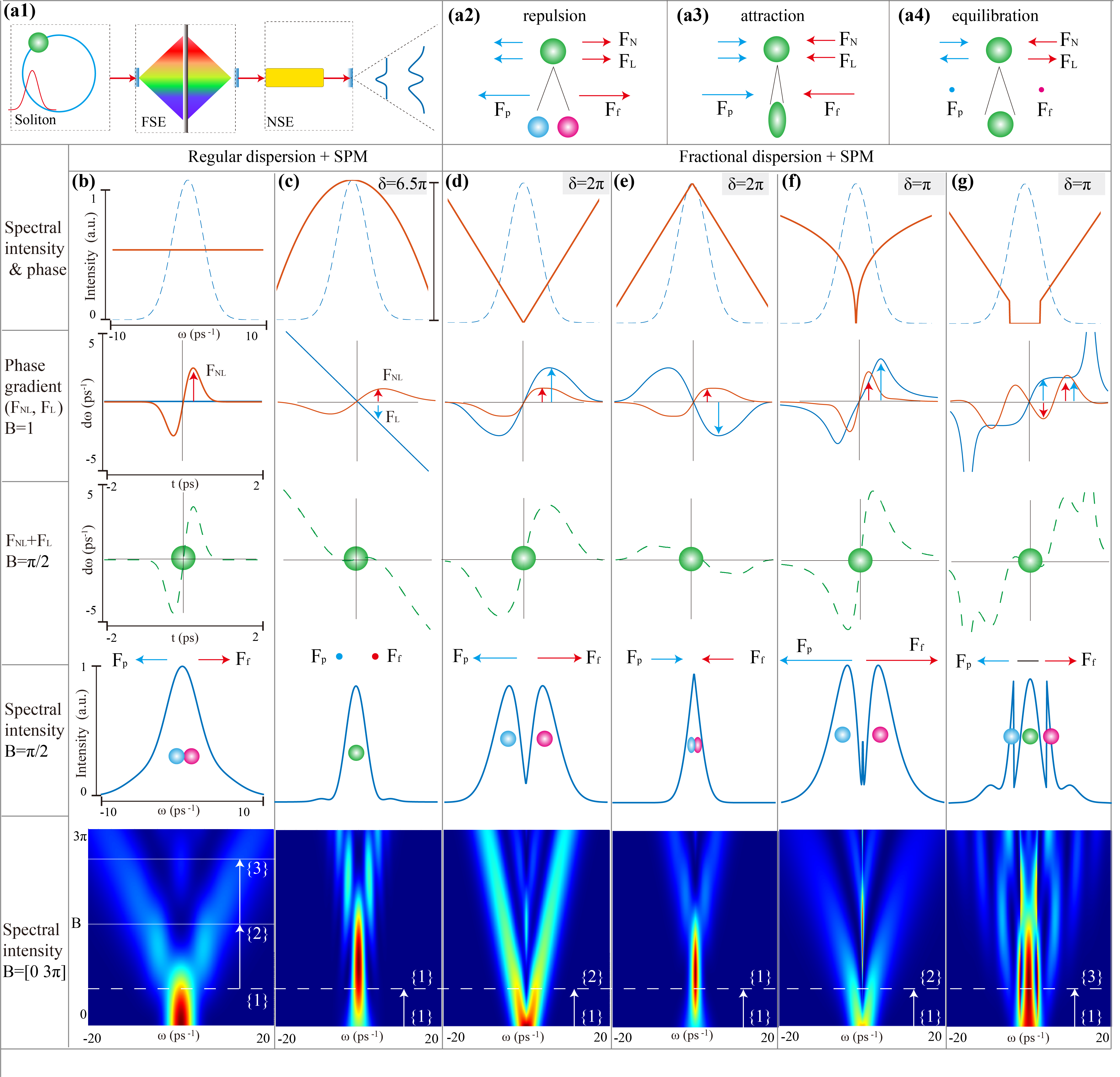
Figure 1 illustrates the concept of spectral bifurcation arising from the interplay between fractional GVD and SPM. In Figure 1(a1), a schematic of the experimental setup is presented. It includes a home-made mode-locked fiber laser (MLF) producing the soliton pulse [20], a pulse shaper (PS) indicating the regular or fractional GVD (labeled as ‘FSE’ in Figure 1(a1)), a gain fiber responsible for inducing both SPM and pulse amplification, and an attached single-mode fiber (‘NSE’ in Figure 1(a1)). Additional details are provided in Methods [M1: The setup for the realization of FNLSE and spectral bifurcation].
As previously stated, the interplay between the forces and results in ‘repulsion’, ‘attraction’, and ‘equilibration’. In the repulsion scenario, depicted in Fig. 1(a2), both forces and act in the same direction, leading to their combined contributions and pushing away from the central part. This results in a stretching of the soliton into a blue- and red-shifted part. Conversely, when their combined contributions converge towards the center, as exemplified in Fig. 1(a3), the combined attraction force results in spectral squeezing. In instances where the forces balance each other out, resulting in a net zero contribution, the shape of the spectrum is conserved (named as equilibration). This is indeed the condition of the formation of soliton, where the total frequency chirp from GVD dispersion and SPM reach a balance. Using this model, it becomes possible to not only predict the behavior of spectral intensity within the framework of FNLSE but also to devise strategies for generating bifurcations with multiple peaks. For consistency, we define a bifurcation mode as {N}, signifying the presence of peaks in the spectral profile.
Figure 1(b) and (c) depict the simulations for the spectrum dynamics under the regular dispersion and SPM. In Figure 1(b), the initial pulse with a flat phase is shown in the first panel. Two forces of and and their sum contribution () are calculated in the second and third panels, respectively. In Figure 1(b), a flat spectral phase is imprinted on the pulse, which means . The fourth panel displays the SI for , and the last panel presents the full SI for varying from 0 to , based on Eq. 5. The sequential emergence of spectral lobes is observed with increase of B, evolving to the bifurcation with two lobes (B=1.5 ) or three lobes (B=2.5 ), as indicated by labels {2} and {3}, respectively. For this case, the relation between the number of lobes N and is approximately given by (=N-0.5) [1]. Typically occurs at higher B values when the spectral phase is non-flat. For example, Figure 1(c) illustrates the scenario where a GVD phase () is loaded into the initial pulse. In this case, the forces and have opposing directions at a small value of , leading to their sum contribution being canceled. This situation is labeled as equilibration, as shown in Figure 1(a4). Nevertheless, with the increase of the nonlinearity, the contribution from plays the main role and also promotes spectral bifurcation. In these SI plots, the dashed white line corresponds to the position of .
In contrast to regular GVD and SPM, significant performances could be achieved in the case of fractional GVD and SPM. In particular, (d) presents the scenario with fractional GVD phase . Here, the alignment of and magnifies the impact of and compared to the default case (a). As a result, substantial frequency shifts occur, leading to the spectral bifurcation even at low values of B, as shown in the fourth and fifth panels of (d). This behavior resembles a repulsive effect. Conversely, if we change the symbol of the fractional GVD phase to , and oppose each other, diminishing the impact of and . This results in a squeezed frequency intensity profile, as depicted in the last panel of (e). Figure 1(f) illustrates the case for smaller LI, i.e., , where a more significant frequency shift occurs at B=. Notably, strong frequency shifts occur for small at small due to the steep spectral phase, which amplifies the force, as shown in the third panel.
Drawing from the three illustrative ‘attraction’, ‘repulsion’, and ‘equilibration’ cases, it becomes conceivable to engineer a more intricate phase structure. For instance, in (g), we configure the initial phase with three distinct segments: the left and right ones adopt the profile , while the central section maintains a flat phase. In this configuration, the left and right sides exhibit ‘repulsion’ effects, while the central portion promotes ‘equilibration’ owing to their interference. In essence, three forces are distributed across the temporal domain, resulting in a bifurcation in the frequency domain with three lobes at B=. This scenario can also manifest itself in the default case of (a), albeit with B set to a higher value, e.g., 2.5 [54]. Utilizing this principle, it becomes feasible to directly create bifurcation modes {N} with multiple lobes, where higher efficiency of the process is reflected at a small value of B, corresponding to weaker nonlinearity.
Further elaboration on the intricacies of the spectral bifurcation can be found in Method-2 (The Temporal Treatment of SPM for the Initial Pulse with Fractional GVD). We provide an approximate analytical expression for the case when =1. Additionally, we delve into an explanation from the frequency domain, specifically the dynamics of the spectral phase. Notably, we observe that the spectral phase induced by SPM undergoes a circular evolution. Initially, it transitions from a regular shape to a fractional one and then reverts back to a regular form. These observations reveal that a complex fractional phase pattern can be employed to generate bifurcations with multiple lobes. These insights are detailed in Supplementary-2 (The Frequency Treatment of SPM for the Initial Pulse with Fractional GVD). For a more comprehensive understanding, supporting movies (refer to Video 1-3) are provided, illustrating the dynamical behavior of spectral intensity and phase under the influence of SPM and fractional phase engineering. These visual aids offer a deeper and visual insight into the intricate dynamics at play.
In the next sections, we present experiments showcasing the realization of spectral bifurcations through the control of the LI , which governs the process. We start by engineering a single jump {1} {2}, and subsequently demonstrate the versatility of the bifurcation engineering of the transition {1} {N} by employing multiple LI values in one single hologram. Lastly, we exhibit a practical application of spectral bifurcations - dense encoding and data squeezing - achieved by transmitting bifurcation modes through a 100-km-long fiber.
Result 2: Experimental realization of FNLSE and spectral bifurcations from {1} to {2}
An effective setup is prepared to realize the aforementioned FNLSE. Three key parts are built: the mode locked fiber laser producing femtosecond soliton pulses; the linear pulse shaper (PS) to engineer dispersion; and a nonlinear environment to perform amplifier and SPM, respectively. To observe spectral dynamics in such frameworks, as anticipated by Eq. 5, the pump power is adjusted to augment the pulse energy, consequently increasing the pulse peak power and B value. For further insights and experimental specifics, refer to Section M1 in Methods.
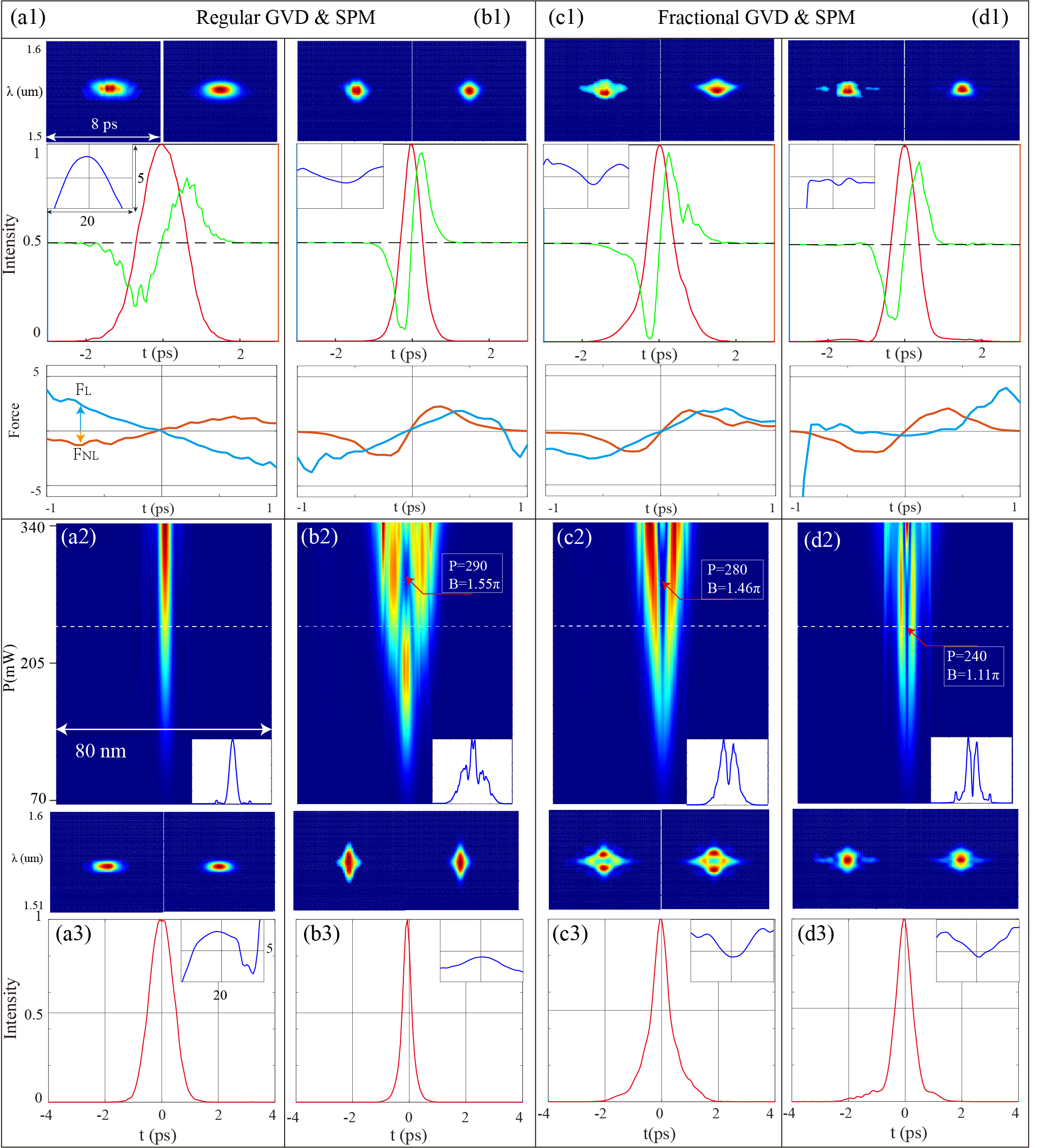
We initially maintain a pump power of 70 mW and manipulate the spectral phase via the hologram in the PS. The primary spectral phase is flat, denoted as , following the definition in Section 1. In this configuration, the soliton pulse passes through the PS without additional spectral modulation. We conducted FROG measurements on the initial soliton pulse. The measured and reconstructed FROG traces are presented in Fig. 2(a1). The reconstructed pulse duration is ca. 810 fs. The reconstructed spectral phase is shown in the top left panel, approximately following a second-order distribution , corresponding to a second-order GVD. This phase results from the fibers and optical elements in the setup, which can be cancelled by adding a second-order spectral phase using the PS (This can be confirmed through FROG results, as shown in Supplementary -3). Our tests indicate that the pulse duration is minimized when the additional GVD phase is about 1.7 times the dispersion length. The corresponding reconstructed intensity profile is depicted in Fig. 2(b1), with a minimal pulse duration of approximately 353 fs. It is evident that the reconstructed spectral phase (inserted panel) is more flattened than the case of (a1).
Figures 2(c1) and (d1) portray scenarios where the spectral phase follows the fractional GVD, i.e., and , respectively. These fractional phases can be validated through the reconstruction results shown in the inserted panels of Figs. 2 c(1) and d(1). The profiles of these phases align with the simulations in Fig. 1, indicating that the intensity and phase gradient forces and , satisfy the requirements for engineering the bifurcation on the initial pulse. The reconstructed forces are displayed in the third panel of Fig. 2 (a1) to (d1). In the case of (a1), ‘equilibration’ is illustrated, where two forces cancel out along the x-axis. By adding the compensated GVD phase, the force of inverts, allowing for the observation of the typical spectrum induced by SPM. The third panel depicts increased contributions from the two forces due to the fractional GVDs as shown in (c1) and (d1). Consequently, spectral bifurcations are observed at smaller values of in the repulsive scenario. The attractive case was also observed in experiments, it is not presented here as the focus is on addressing spectral bifurcations.
The next step involves fixing the spectral phase and recording the spectral intensity (SI) while varying the pump power, effectively changing the value of B. In Figs. 2(a2) and (b2), the recorded SI is displayed for the initial pulse with regular GVD from the PS. In Fig. 2(a2), the SPM-induced variations in SI are subtle due to pulse broadening. However, the SPM effect becomes evident when the pulse duration is minimized as shown in Fig. 2(b1), where an interference dip emerges around 290 mW, corresponding to B being approximately (The pump power - B relation can be found in Section M1 of Methods). As per the relationship between the number of lobes and the maximum phase shift [1], the theoretical B value should be . However, this threshold can be lowered when the initial pulse is modulated by fractional GVD. For instance, Figs. 2(c2) and (d2) show the recorded SI for and , respectively, revealing a pronounced bifurcation dip even at lower pump powers, 280 mW (B= ) and 240 mW (B= ), respectively. As decreases, the deepest point of the bifurcation occurs at smaller B values. We fixed the pump power to 240 mW and recorded one-dimensional normalized distributions of SI as shown in the lower right corner of Figs. 2(a2)-(d2). It can be seen that one strong bifurcation with two lobes is distinctly visible in the case of fractional GVD. The FROG traces are presented above in Figs. 2(a3)-(d3), and the corresponding temporal intensity and spectral phase are shown in Figs. 2(a3)-(d3). These experimental findings align with the simulations presented in Section 1, and they are consistent with the explanations provided by the force model. Notably, a global GVD phase, approximately twice the GVD dispersion length, is added to the fractional GVD phase to enhance the bifurcation dip. This addition helps to balance or amplify the force , as demonstrated in Fig. 2 (a1).
Result 3: Spectral bifurcations from {1} to {N}
Utilizing the force model outlined in Section 1, we establish an approximate on-demand mapping between the spectral phase and spectral intensity (SI) in SPM. While the exact relationship may require solutions from FNLSE or simulations involving Eq. 4 and Eq. 5, this approximate approach allows us to efficiently design segmented fractional spectral phases for generating bifurcation modes from {1} to {N}.
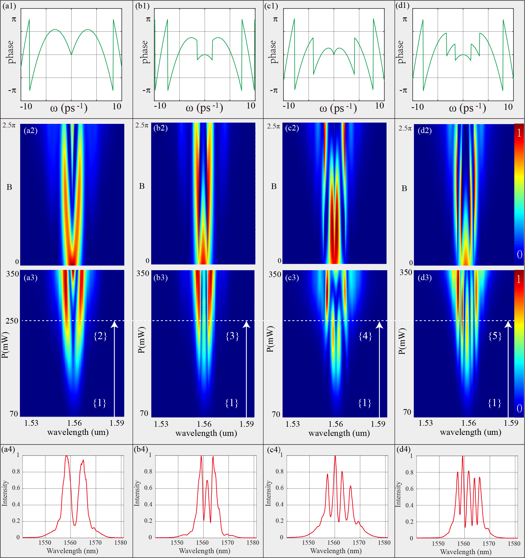
The required fractional spectral phase pattern wrapped between to is shown in Fig. 3(a1) for the generation of bifurcation modes from {1} to {2}, in which the fractional part encompasses LI :
| (9) |
In line with this fractional phase, we show the theoretical and experimental SI varying or the pump power as shown in Fig. 3(a2) and (a3), respectively. The normalized SI for the pump power 250 mW is plotted in the last panel of Fig. 3(a1). Two lobes are clearly observed in SI.
To create the bifurcation with three lobes, we set the segmented spectral phase in the hologram to carry a fractional and constant phase in adjacent sections, based on the force model:
| (10) |
where is the central wavelength. Adding a global GVD phase to this segmented phase pattern yields the final phase configuration, showcased in Fig. 3(b1). When this phase is imposed on the SLM, three lobes are formed in SI with the increase of pump power, as displayed in simulations in Fig. 3(b2), and experimental measurements in Fig. 3(b3), respectively. Notably, three lobes emerge in both cases even for relatively small B values. As the pump power increases further, the two side lobes retain greater intensity than the central one, subsequently fading out due to interference effects. This behavior aligns with the force model, where the unique phase distribution contributes to the emergence of three lobes: the lateral lobes are generated by a repulsive force, while the central segment preserves the original state due to the Equilibration, as described in the right-hand side of Eq. 10.
Figures 3(c1) to (c4) illustrate the scenario of a bifurcation mode of {4}, achieved by dividing the phase configuration into four segments based on their force interactions. This design involves two fractional terms with LIs of 0.5 and 1, respectively. Notably, the total force exerted by the LI 0.5 segment needs to be weaker than that of the LI 1 segment. The required fractional GVD phase is expressed as follows:
| (11) |
Upon loading the required spectral phase onto the initial pulse, a four-lobe pattern emerges within the pump power range of 70 to 250 mW, as depicted in Fig. 3 (c3). Subsequently, due to interference, the two central lobes disappear, potentially reappearing with a further increase in pump power. We don’t show the results at higher powers because of the potential occurrence of gain saturation [55].
More lobes could be realized by partitioning the fractional phase into more segments. This entails designing a multi-functional force distribution, encompassing attributes such as ‘equilibration’, ‘weak repulsion’, and ‘strong repulsion’. To realize this, the spectral phase configuration is arranged as follows:
| (12) |
The spectral phase configuration is displayed in Figs. 3(d1), where five segmented phases are observed. Loading this phase onto PS and subsequently altering the pump power results in SI variations, as displayed in Figs. 3(d3). Experimental observations confirm that this segmented phase design induces a spectral bifurcation with five lobes.
To provide clearer visibility of these bifurcations, we have plotted the one-dimensional normalized spectral intensity for a consistent pump power of approximately 250 mW, as demonstrated in Figs. 3(a4) to (d4). The number of spectral lobes is in direct correlation with the designed numbers embedded in the spectral phase. Notably, these outcomes align well with the force model. It is intriguing to observe that these spectral intensity patterns exhibit a strong resemblance to the one-dimensional Hermite-Gauss temporal mode, [56], particularly in terms of the number of peaks. Further optimization of the spectral phase could potentially enhance these resemblances.
Both in simulations and experiments, we introduced an additional second-order GVD phase term, approximately 3.37 times the dispersion length, as a foundational global phase for the designed fractional-GVD pattern. This global phase serves a dual purpose: it counterbalances the added dispersion caused by the optical setup and enhances the suitable temporal chirp (referred to as ) for more pronounced interference with a deeper dip. Additionally, these phase profiles as shown in Fig. 3 (a1)-(d1), closely resemble the spectral phase generated by SPM in simulations, particularly the peak segment [See Supplementary -2 and the videos in supporting materials]. In the SI simulations in Fig. 3 (a2)-(d2), we imposed the conservation of input spectral energy, consistent with the experimental settings. Also, in the experiment, the presence of Kelly sidebands in the spectra of soliton pulses from MLF requires pre-removal to prevent crosstalk in SI. This was accomplished by incorporating a bandpass filter into the hologram (See the results in Supplementary- 4).
Result 4: The applications of the spectral bifurcations mode in data squeezing
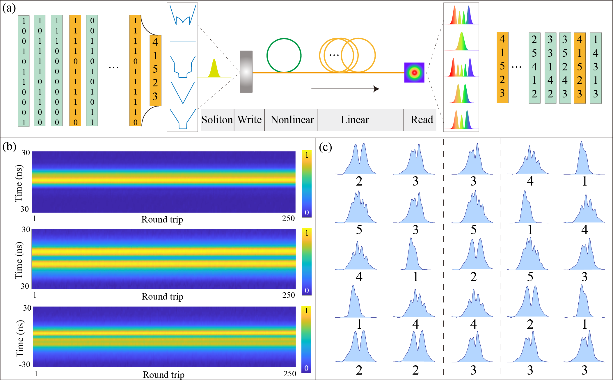
In the experimental results presented in Figure 3, two relevant features are observed. First, by adjusting the spectral phase suitably in the hologram, bifurcations with multiple lobes can be achieved. Second, these bifurcation modes can be created at the same nonlinearity, or the same pump power, which is beneficial and convenient for optical signal processing. A promising possibility is to apply these bifurcation modes to optical signal dense encoding and transmission. Traditional optical transmission systems use binary encoding, i.e., ‘0’ or ‘1’. However, the creation of five bifurcation modes goes beyond binary encoding, allowing a quinary regime. Figure 4 demonstrates data squeezing from binary to quinary by using five spectral bifurcation modes {1} to {5}, where {1} is the fundamental mode illustrated in Fig. 2 (a2).
To perform the data encoding and squeezing, the first step is to transform the binary data into the quinary as shown in the left part of Fig. 4 (a). These quinary data ({25412 ,33142 ,35243 ,41523 ,14313}) are then encoded in sequence into the aforementioned five spectral phases, which represent a ‘write’ process. In the second step, the pump power is fixed at around 250 mW, and the corresponding spectral bifurcation mode is generated under the SPM. The signal is then transmitted through around 100 km of fiber named ‘linear’ and detected by a photodetector and oscilloscope named ‘read’, respectively. Due to the effect of the group delay dispersion (GDD), induced by the long fiber, the measured stretched temporal profiles in the oscilloscope are proportional to the spectral intensity [11, 46, 20]. In the last step, the peak numbers in these profiles are counted and the data is decoded from quinary to binary.
Figure 4 (b) shows the stretched temporal profiles recorded on the oscilloscope for bifurcation modes of {1}, {2}, and {3}. The stretched temporal profiles demonstrate robustness over 250 round trips, and a dip is clearly observed at the center of the profile for these modes. Fig. 4 (c) shows one of the output profiles with 25 holograms that encode the above-mentioned complex phase. By counting the number of peaks in these profiles, we obtain the same sequence. It should be noted that the dips for the bifurcation mode of {3} to {5} are not very deep, mainly limited to the low sampling rate and the temporal resolution of the oscilloscope. In addition, the higher-order GVD in the 100 km fiber affects these profiles. Nevertheless, the results demonstrate that these spectral bifurcations offer great potential applications to optical signal processing, particularly for data squeezing. For example, using the quinary regime can reduce the number of pulses in optical signal communications to while maintaining the data throughput.
Discussion
In this work, we have experimentally investigated the spectral dynamics influenced by fractional GVD (group velocity dispersion) and SPM (self-phase modulation) with respect to the model based on the FNLSE (fractional nonlinear Schrödinger Equation). In the presence of both nonlinear effects and dispersion in the FNLSE, obtaining a comprehensive theoretical solution is challenging. To gain insights into the effect of strong frequency splitting observed in the spectral dynamics, we introduced a force model with ‘repulsion’, ‘attraction’, and ‘equilibration’ to explain the interplay between the fractional dispersion and SPM. With the help of the proposed model, we have successfully prepared the segmented fractional phase and produced the bifurcation modes directly from {1} to {N} realized in the femtosecond soliton pulse, which goes beyond the traditional sequential bifurcation pattern, e.g., {1}{2}{3} …{N}). As such, access to rich spectral and temporal pulse profiles is obtained on demand by arbitrary jumps {1} {N} simply by loading appropriate phase profiles. This represents an efficient way for tailoring optical nonlinearity.
To illustrate exemplary utility of our approach, we demonstrated use of these spectral bifurcation modes for the optical data dense encoding and transfer. Specifically, we used five bifurcation modes of the pulse to achieve optical data squeezing from binary to quinary formats transmitting over 100-km-long single-mode fiber. Although the switching speed is currently limited by the low speed of the spatial light modulator (SLM) in the pulse shaper, the results highlight the potential of these bifurcation modes in optical signal processing. Operational speed can be readily improved by using an electro-optic modulator as time-domain shaper [57]. Moreover, the high brightness and structured nature of the spectral bifurcation modes hold promise for applications in temporal mode quantum optics and information [56].
Finally, we want to emphasize that the spectral bifurcation reported in this work is just one aspect of the FNLSE, and there are other fruitful avenues for the studies. One potentially promising topics is to map out other solutions of FNLSE, such as fractional solitons or atoms [52, 43, 24]. Another interesting aspect to explore is the generation of spectral bifurcation with more lobes by manipulating more complex dispersion phases and selecting pulses with larger bandwidths. This may find potential applications to the generation of frequency combs, which are widely used in various fields [31]. Furthermore, investigating pulse dynamics under the action of stronger nonlinearity is an intriguing perspective. This may shed light on the supercontinuum generation in the framework of the FNLSE, offering new possibilities for the design of broadband light sources and nonlinear optical phenomena [4].
Methods
2: The temporal treatment of SPM for the initial pulse with the fractional GVD
Generally, under the approximation of the short length of the nonlinear fiber and ignoring the dispersion effect, the evolution of under the action of SPM is provided by
| (13) |
To get the spectral intensity, we perform the Fourier transform of Eq. 13:
| (14) |
It is difficult to get an analytical expression for the spectral intensity defined in Eq. 13. Therefore, one usually tries to analyze the frequency chirp induced by SPM. In our case, the fractional GVD would strongly revise not only the temporal profile but also the temporal phase. Therefore, we rewrite the Eq. 13 to the new form:
| (15) |
The temporal phase induced SPM in Eq. 15 produces a superposed frequency chirp:
| (16) |
Where, , , and similarly the force produces a new frequency shift [53], in which is the normalized temporal intensity, and comes from the contribution of the pulse shaper. The superposed force, , indicated the total force, which means the total frequency chirp.
Let’s consider one Gaussian spectral amplitude with the fractional GVD phase, i.e.,
| (17) |
Here, is relative to the bandwidth; defines the strength of fractional phase united by the fractional dispersion length . For similarity, we set the and get the initial temporal filed:
| (18) |
Here . The temporal intensity could be seen as a superposition of two symmetric Gaussian wavepacket and [58, 49].
Therefore, the temporal intensity () could get
| (19) |
The temporal phase gives:
| (20) |
Two temporal phases produce the force defined in Eq. 16. Regarding , it gives
| (21) |
And :
| (22) |
Therefore, the superposed force, , could be obtained by Eq. 21 and Eq. 22. The advance is not necessary to perform the Fourier transform in calculations; therefore, it doesn’t need to consider the limitation on the temporal window and resolution during simulations.
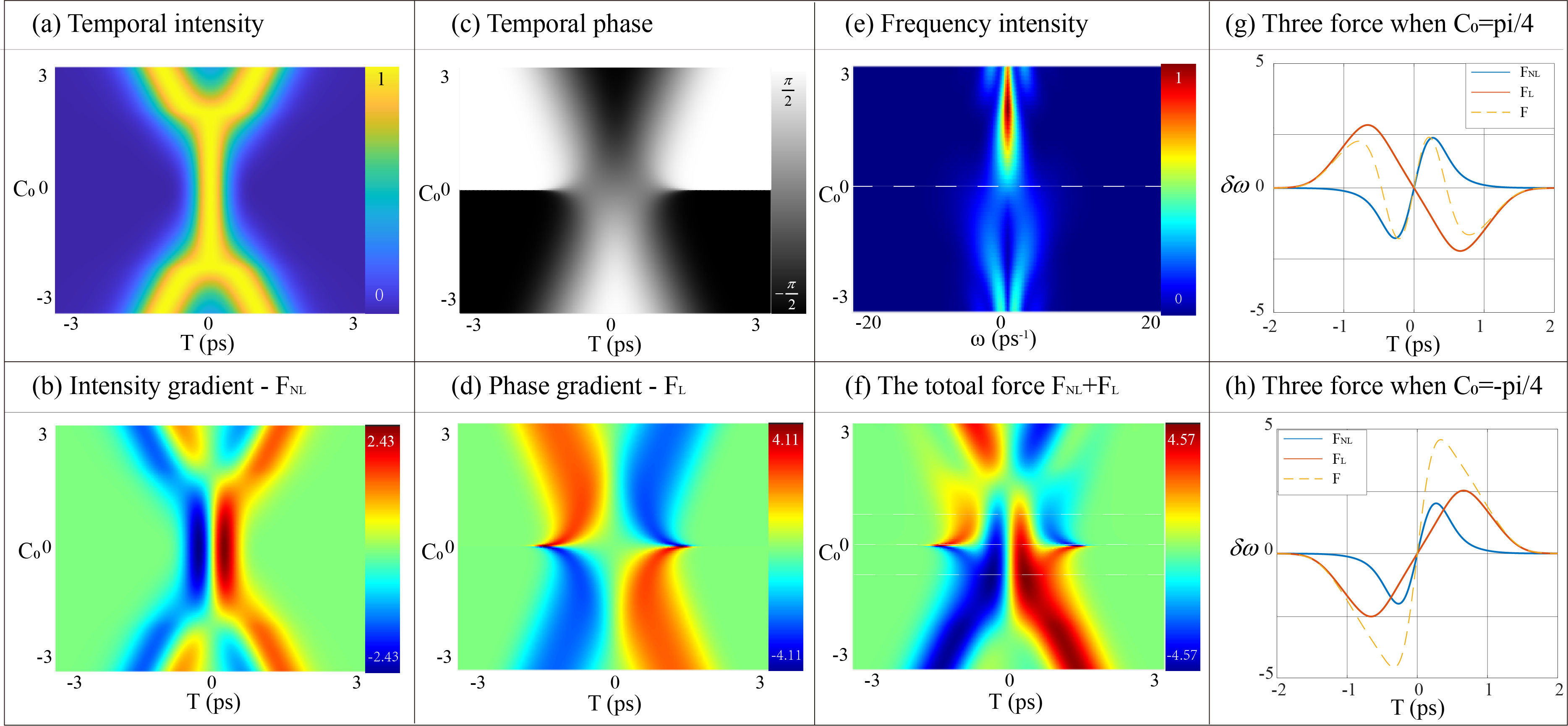
is associated with fractional GVD coefficient and bandwidth . We fix to be a constant, i.e., 4 in the following simulations, and study the relation between and time , that is . Fig. 5 gives the simulations of the initial pulse defined by a Gaussian spectrum, cft., Eq.17, here, we set the parameter from -3 to 3; time from -3 to 3 ps, and .
Fig. 5(a) shows the normalized temporal intensity defined in Eq. 19 for from -3 to 3. As the increase of from absolutely 0 to 3, the pulse duration becomes broader and the pulse splits beyond around . The intensity gradient, , is calculated and shown in Fig. 5(b). The distribution of the temporal phase and the corresponding are shown in (c) and (d), respectively. In the temporal phase, it could be seen that the phase distribution is inverted for and , respectively. This is reasonable upon the definition of fractional GVD in Eq. 17. This unique phase makes the inverted not only along the y-axis but also along the x-axis direction. By adding and , we get the total force of , which is shown in Fig. 5(f). It could be seen that two clear branches appear for , and multiple branches arise for . To verify the spectrum, Fig. 5(e) gives the corresponding spectral intensity under the different , where we calculate them by Fourier transform defined by Eq. 14· The simulations illustrate that the bifurcation is more clear for in comparison with the case of .
Specifically, Fig. 5 (g) and (h) show the one-dimensional distribution for forces of , , and , where is set to be and , respectively. The absolute value of could be up to maximum when is set to around . This also could be verified in (h), where the blue, red solid line and dashed line represent , , and , respectively. In this case, two forces have the co-direction, so the contribution enhances the final force, showing ‘repulsion’, and thus promotes the larger frequency shift. Fig. 5(g) shows one case for setting . In this case, two forces have counter-direction, and the contribution from them is closed to be canceled, showing ‘equilibration’. In other words, the final force is inverted, producing a tiny frequency shift. For the case of , the contribution from is zero, and one is doing solely with the contribution from SPM, that is .
Data availability
The data that support the findings of this study are available from the corresponding authors, S.L. (dr.shilongliu@gmail.com) or D. V. S. (denis.seletskiy@polymtl.ca), upon reasonable request.
References
- [1] Agrawal, G. P. Nonlinear fiber optics. In Nonlinear Science at the Dawn of the 21st Century, 195–211 (Springer, 2000).
- [2] Boyd, R. W. Nonlinear optics (Academic press, 2020).
- [3] Solli, D. R., Ropers, C., Koonath, P. & Jalali, B. Optical rogue waves. \JournalTitleNature 450, 1054–1057 (2007).
- [4] Dudley, J. M., Genty, G. & Coen, S. Supercontinuum generation in photonic crystal fiber. \JournalTitleRev. Mod. Phys 78, 1135 (2006).
- [5] Skryabin, D. V. & Gorbach, A. V. Colloquium: Looking at a soliton through the prism of optical supercontinuum. \JournalTitleRev. Mod. Phys. 82, 1287 (2010).
- [6] Fermann, M. E., Kruglov, V., Thomsen, B., Dudley, J. M. & Harvey, J. D. Self-similar propagation and amplification of parabolic pulses in optical fibers. \JournalTitlePhys. Rev. Lett. 84, 6010 (2000).
- [7] Dudley, J. M., Finot, C., Richardson, D. J. & Millot, G. Self-similarity in ultrafast nonlinear optics. \JournalTitleNature Physics 3, 597–603 (2007).
- [8] Teğin, U., Kakkava, E., Rahmani, B., Psaltis, D. & Moser, C. Spatiotemporal self-similar fiber laser. \JournalTitleOptica 6, 1412–1415 (2019).
- [9] Biesenthal, T. et al. Fractal photonic topological insulators. \JournalTitleScience 376, 1114–1119 (2022).
- [10] Goda, K., Tsia, K. & Jalali, B. Serial time-encoded amplified imaging for real-time observation of fast dynamic phenomena. \JournalTitleNature 458, 1145–1149 (2009).
- [11] Mahjoubfar, A. et al. Time stretch and its applications. \JournalTitleNat. Photonics 11, 341 (2017).
- [12] Solli, D., Chou, J. & Jalali, B. Amplified wavelength–time transformation for real-time spectroscopy. \JournalTitleNature Photonics 2, 48–51 (2008).
- [13] Rao DS, S. et al. Shot-noise limited, supercontinuum-based optical coherence tomography. \JournalTitleLight: Science & Applications 10, 133 (2021).
- [14] Agrell, E. et al. Roadmap of optical communications. \JournalTitleJournal of Optics 18, 063002 (2016).
- [15] Genty, G. et al. Machine learning and applications in ultrafast photonics. \JournalTitleNat. Photonics 15, 91–101 (2021).
- [16] Teğin, U., Yıldırım, M., Oğuz, İ., Moser, C. & Psaltis, D. Scalable optical learning operator. \JournalTitleNature Computational Science 1, 542–549 (2021).
- [17] Zhou, T., Wu, W., Zhang, J., Yu, S. & Fang, L. Ultrafast dynamic machine vision with spatiotemporal photonic computing. \JournalTitleScience Advances 9, eadg4391 (2023).
- [18] Grelu, P. & Akhmediev, N. Dissipative solitons for mode-locked lasers. \JournalTitleNat. Photonics 6, 84–92 (2012).
- [19] Krupa, K., Nithyanandan, K., Andral, U., Tchofo-Dinda, P. & Grelu, P. Real-time observation of internal motion within ultrafast dissipative optical soliton molecules. \JournalTitlePhys. Rev. Lett. 118, 243901 (2017).
- [20] Liu, S., Cui, Y., Karimi, E. & Malomed, B. A. On-demand harnessing of photonic soliton molecules. \JournalTitleOptica 9, 240–250 (2022).
- [21] Malomed, B. A. Bound solitons in the nonlinear schrödinger/ginzburg-landau equation. In Large Scale Structures in Nonlinear Physics, 288–294 (Springer, 1991).
- [22] Akhmediev, N., Ankiewicz, A. & Soto-Crespo, J. Multisoliton solutions of the complex ginzburg-landau equation. \JournalTitlePhys. Rev. Lett. 79, 4047 (1997).
- [23] Kivshar, Y. S. & Agrawal, G. P. Optical solitons: from fibers to photonic crystals (Academic press, 2003).
- [24] Malomed, B. A. Multidimensional solitons (2022).
- [25] Mollenauer, L. F., Stolen, R. H. & Gordon, J. P. Experimental observation of picosecond pulse narrowing and solitons in optical fibers. \JournalTitlePhys. Rev. Lett. 45, 1095 (1980).
- [26] Boscolo, S. & Finot, C. Shaping light in nonlinear optical fibers (John Wiley & Sons, 2017).
- [27] Tzang, O., Caravaca-Aguirre, A. M., Wagner, K. & Piestun, R. Adaptive wavefront shaping for controlling nonlinear multimode interactions in optical fibres. \JournalTitleNature Photonics 12, 368–374 (2018).
- [28] Shimizu, F. Frequency broadening in liquids by a short light pulse. \JournalTitlePhys. Rev. Lett. 19, 1097 (1967).
- [29] Stolen, R. H. & Lin, C. Self-phase-modulation in silica optical fibers. \JournalTitlePhysical Review A 17, 1448 (1978).
- [30] Qin, L. Optical frequency metrology 003. \JournalTitleNature 416, 233–237 (2002).
- [31] Ye, J. & Cundiff, S. T. Femtosecond optical frequency comb: principle, operation and applications (Springer Science & Business Media, 2005).
- [32] Apolonski, A. et al. Controlling the phase evolution of few-cycle light pulses. \JournalTitlePhys. Rev. Lett. 85, 740 (2000).
- [33] Riek, C. et al. Subcycle quantum electrodynamics. \JournalTitleNature 541, 376–379 (2017).
- [34] Virally, S., Cusson, P. & Seletskiy, D. V. Enhanced electro-optic sampling with quantum probes. \JournalTitlePhys. Rev. Lett. 127, 270504 (2021).
- [35] Riek, C. et al. Direct sampling of electric-field vacuum fluctuations. \JournalTitleScience 350, 420–423 (2015).
- [36] Soto-Crespo, J. M., Akhmediev, N. & Ankiewicz, A. Pulsating, creeping, and erupting solitons in dissipative systems. \JournalTitlePhys. Rev. Lett. 85, 2937 (2000).
- [37] Dudley, J. M. & Taylor, J. R. Ten years of nonlinear optics in photonic crystal fibre. \JournalTitleNature Photonics 3, 85–90 (2009).
- [38] Bell, B. A. et al. Spectral photonic lattices with complex long-range coupling. \JournalTitleOptica 4, 1433–1436 (2017).
- [39] Laskin, N. Fractional quantum mechanics. \JournalTitlePhys. Rev. E 62, 3135 (2000).
- [40] Laskin, N. Fractional quantum mechanics and lévy path integrals. \JournalTitlePhys. Lett. A 268, 298–305 (2000).
- [41] Longhi, S. Fractional schrödinger equation in optics. \JournalTitleOpt. Lett. 40, 1117–1120 (2015).
- [42] Zhang, Y. et al. Propagation dynamics of a light beam in a fractional schrödinger equation. \JournalTitlePhys. Rev. Lett. 115, 180403 (2015).
- [43] Malomed, B. A. Optical solitons and vortices in fractional media: A mini-review of recent results. In Photonics, vol. 8, 353 (Multidisciplinary Digital Publishing Institute, 2021).
- [44] Zhang, Y. et al. Pt symmetry in a fractional schrödinger equation. \JournalTitleLaser & Photonics Rev. 10, 526–531 (2016).
- [45] Ming Zhong, Z. Y. Spontaneous symmetry breaking and ghost states in two-dimensional fractional nonlinear media with non-hermitian potential. \JournalTitleCommunications Physics 6 (2023).
- [46] Cui, Y. et al. Xpm-induced vector asymmetrical soliton with spectral period doubling in mode-locked fiber laser. \JournalTitleLaser & Photonics Reviews 15, 2000216 (2021).
- [47] Li, P., Malomed, B. A. & Mihalache, D. Symmetry-breaking bifurcations and ghost states in the fractional nonlinear schrödinger equation with a pt-symmetric potential. \JournalTitleOptics Letters 46, 3267–3270 (2021).
- [48] Li, P. et al. Second-harmonic generation in the system with fractional diffraction. \JournalTitleChaos, Solitons & Fractals 173, 113701 (2023).
- [49] Liu, S., Zhang, Y., Malomed, B. A. & Karimi, E. Experimental realisations of the fractional schrödinger equation in the temporal domain. \JournalTitleNature Communications 14, 222 (2023).
- [50] Bayın, S. Ş. Definition of the riesz derivative and its application to space fractional quantum mechanics. \JournalTitleJournal of Mathematical Physics 57, 123501 (2016).
- [51] Driben, R. & Malomed, B. A. Split-step solitons in long fiber links. \JournalTitleOptics communications 185, 439–456 (2000).
- [52] Laskin, N. Fractional Quantum Mechanics (World Scientific: Singapore, 2018).
- [53] Zheltikov, A. The lagrangian structure, the euler equation, and second newton’s law of ultrafast nonlinear optics. \JournalTitleOptics Communications 129766 (2023).
- [54] Agrawal, G. P. & Potasek, M. Nonlinear pulse distortion in single-mode optical fibers at the zero-dispersion wavelength. \JournalTitlePhysical Review A 33, 1765 (1986).
- [55] Ilday, F., Buckley, J., Clark, W. & Wise, F. Self-similar evolution of parabolic pulses in a laser. \JournalTitlePhys. Rev. Lett. 92, 213902 (2004).
- [56] Brecht, B., Reddy, D. V., Silberhorn, C. & Raymer, M. G. Photon temporal modes: a complete framework for quantum information science. \JournalTitlePhys. Rev. X 5, 041017 (2015).
- [57] Yao, J. Photonic generation of microwave arbitrary waveforms. \JournalTitleOptics Communications 284, 3723–3736 (2011).
- [58] Vogt, G. et al. Analysis of femtosecond quantum control mechanisms with colored double pulses. \JournalTitlePhys. Rev. A 74, 033413 (2006).