Choosing Wisely and Learning Deeply: Selective Cross-Modality Distillation via CLIP for Domain Generalization

Abstract

Domain Generalization (DG), a crucial research area, seeks to train models across multiple domains and test them on unseen ones. In this paper, we introduce a novel approach, namely, Selective Cross-Modality Distillation for Domain Generalization (SCMD). SCMD leverages the capabilities of large vision-language models, specifically the CLIP model, to train a more efficient model, ensuring it acquires robust generalization capabilities across unseen domains.

Our primary contribution is a unique selection framework strategically designed to identify hard-to-learn samples for distillation. In parallel, we introduce a novel cross-modality module. This module seamlessly combines the projected features of the student model with the text embeddings from CLIP, ensuring the alignment of similarity distributions.

We assess SCMD’s performance on various benchmarks, where it empowers a ResNet50 to deliver state-of-the-art performance, surpassing existing domain generalization methods. Furthermore, we provide a theoretical analysis of our selection strategy, offering deeper insight into its effectiveness and potential in the field of DG.

1 Introduction

Imagine a young pianist learning to perform a complex piece of music. Initially, she listens to her experienced piano teacher’s rendition, absorbing the nuances and techniques. Yet, the most crucial learning comes from recording and listening to her own performances. When she listens to her own recordings, she can identify where her performance differs from the perfect melody she has in mind - the ideal, real-world performance. These differences are more valuable for her improvement than simply comparing her performance to the ideal. This is because these disparities directly reflect her unique challenges, and addressing them (with the teacher’s help) will have the most direct impact on improving her performance.

This learning scenario is akin to the process of Knowledge Distillation [1]. The simpler problems that the pianist initially tackles resemble the easily learnable features of a dataset, which a student model can grasp without assistance. The complex music pieces, however, symbolize the hard-to-grasp parts of the data, where the student model benefits immensely from the teacher model’s guidance.

As the pianist matures artistically, she discerns that mastering known pieces alone does not capture the full essence of her musical journey. Wanting to elevate her compositions, she begins to intertwine lyrics into her melodies. This is not a mere juxtaposition of words and tunes; it is a realization that lyrics can heighten the clarity and expressiveness of her music. In the same vein, the harmonization of visual content and natural language in the CLIP model is not just for the sake of fusion, but because language can significantly augment the nuances of visual recognition.

Deep learning models, much like the pianist, might occasionally struggle when exposed to unfamiliar terrains or “genres” in the form of out-of-domain data. Despite the proficiency of deep learning in various tasks, they can often falter when faced with such “novel compositions”. This situation frequently arises in real-world applications. Numerious algorithms have been developed to ensure consistency across distributions [2, 3] and regularize the models to learn domain-invariant features [4, 5, 6], but they often yield only modest improvements [7] over traditional Empirical Risk Minimization (ERM) technique [8].

Inspired by the pianist’s pursuit of harmony between melody and lyrics, and her introspective approach to identify discrepancies in her performance to perfect her craft, our work similarly seeks to focus on challenging aspects of training data and incorporate semantic information to better capture the domain-invariant features. In this paper, we present the Selective Cross-Modality Distillation (SCMD) framework.

Rather than relying on the soft target distribution from the teacher model, SCMD emphasizes the discrepancies, specifically, the gap between the student’s performance and real-world expectations. Just as the pianist hones in on the variations between her rendition and the ideal composition, SCMD selects hard-to-learn samples in the training data, targeting those for knowledge distillation. This approach, we believe, not only enhances the learning process, but also arms the student model with robust feature representations, crucial for navigating unfamiliar terrains.

We have chosen to utilize the CLIP model as a key component of our approach, not only for its ability to combine visual and linguistic information, but mainly for its proficiency in matching images with textual descriptions. This special capacity of CLIP enhances our framework, offering a more comprehensive knowledge base from which our student models can extract and learn.

Contributions:

• We present the Selective Cross-Modality Distillation (SCMD) framework, an innovative departure from traditional methods, emphasizing adaptive sample treatments over the uniform approaches commonly found in current knowledge distillation techniques.

• We underscore the significance of intricate and hard-to-learn training samples and provide a comprehensive theoretical foundation for our selection strategies.

• We propose a cross-modality distillation module within our SCMD framework to leverage the unique capabilities of the CLIP model, seamlessly integrating linguistic comprehension with visual perception for a more nuanced learning paradigm.

• We substantiate the effectiveness of our SCMD method through empirical evaluations, demonstrating its superior performance and capability to establish new standards on the various benchmarks.

2 Related Work

2.1 Domain Generalization

Domain Generalization (DG) [9] has recently emerged as a key area in machine learning, focused on training models with data from multiple source distributions for application on a distinct target distribution. This paradigm has spurred methods for training distribution invariance, either through explicit regularization-based techniques [10, 11, 12, 13, 14, 15, 16, 17, 18, 19] or data augmentation [20, 21, 22, 23, 24, 25], rooted in the assumption that distributional invariance augments model generalization.

DG is generally classified into three facets: data manipulation, representation learning, and learning strategy [26]. Data manipulation [23, 24] refines inputs to facilitate learning generalizable representations. Representation learning techniques [9, 27, 28, 4] aim for domain-invariant feature representations to enhance generalization. Some methods employ learning strategies like meta-learning [29] to simulate domain shifts during training, improving the model’s adaptability to unseen domains. Recent studies indicate that weight averaging can further boost DG task performance [30, 31], contributing to more stable out-of-domain test results.

Several previous studies have leveraged vision-language models to enhance Domain Generalization (DG) performance, closely aligning with our contribution. For instance, Domain Prompt Learning (DPL) [32] employs a lightweight prompt adaptor to automatically generate a prompt estimating domain-specific features from unlabeled examples across distributions. However, these generated prompts often lack clear semantic meanings, potentially limiting their effectiveness in certain contexts [33]. Other research [34] dispatches appropriate pretrained models, including CLIP, to each sample based on their generalization ability. Another approach [35] reformulates the DG objective using mutual information with oracle models, including CLIP.

While numerous domain generalization techniques have been explored in the literature, our approach is unique in that it uses knowledge distillation to achieve this purpose. We show the versatility and potential of knowledge distillation by using CLIP as the teacher model and training a student model afterwards. This combination of ideas, though seemingly straightforward, is a new direction that has not been explored much in prior research.

2.2 Contrastive Language-Image Pre-Training

CLIP [36], a vision-language model, has recently garnered significant attention for its potential to enhance the robustness of machine learning models. Models like CLIP employ a contrastive loss to align visual and text encoders within a shared feature space, demonstrating promise for generic visual representation learning and zero-shot transfer via prompts [36, 37, 38, 39, 40, 41].

Pretraining on 400 million image-text pairs [36] enables CLIP to align semantic meanings between images and sentences, excelling particularly in zero-shot image classification. For instance, it matches a fully-supervised ResNet101 model’s performance with a 76.2% top-1 accuracy rate on the ImageNet [42] validation set and outperforms it on the ImageNet Sketch Dataset with 60.2% accuracy.

CLIP’s exceptional capabilities, derived from pretraining on a vast number of image-text pairs, have shown its prowess especially in tasks like zero-shot image classification. It excels in aligning images and text prompts. Yet, the true potential of such a powerful model lies not just in its standalone performance but in how its extensive knowledge can be transferred to other architectures.

In this paper, we present a novel method to distill knowledge from CLIP, a multi-modal vision-language model, into a single-modal student model. By transitioning from multi-modal to single-modal distillation, we aim to enhance the student model’s domain generalization, opening up new avenues for leveraging these potent models.

2.3 Knowledge Distillation

Knowledge distillation, introduced by Hinton et al. [1], is a pivotal technique for balancing model performance and computational complexity by training a smaller student network with the soft output of a larger teacher model. This approach has spurred extensive research in model compression [43] and knowledge transfer [44].

Numerous distillation techniques have emerged, including feature-based knowledge transfer methods [45, 46, 47, 48, 49] that align embeddings from certain layers, [50] that train teacher and student models concurrently. The design of loss functions operating on the outputs of both models has also been a significant research area, with notable methods including $l_{1}$ [51], $l_{2}$ [52, 53, 54], Maximum Mean Discrepancy (MMD) [55], KL divergence [56, 57, 58], and cross-entropy losses [59, 60].

However, most studies focus on homologous-architecture distillation, leaving cross-architecture distillation relatively untapped. Recently, Liu et al. [61] made significant progress in this area by mapping a CNN’s feature space into a transformer’s attention and feature space using a partially cross-attention projector and a group-wise linear projector. With cross-view robust training, they achieved remarkable performance on ImageNet [42].

Diverging from the norm, our approach offers a fresh perspective on knowledge distillation through two innovations. Firstly, we incorporate a novel selection mechanism that identifies hard-to-learn samples, enhancing the student model’s depth of understanding. Secondly, leveraging on CLIP’s multi-modal capabilities, we employ a cross-modality module. This strategy enables a profound transfer of both visual and linguistic knowledge, greatly enhancing the domain generalization prowess of the student model.

3 Methods

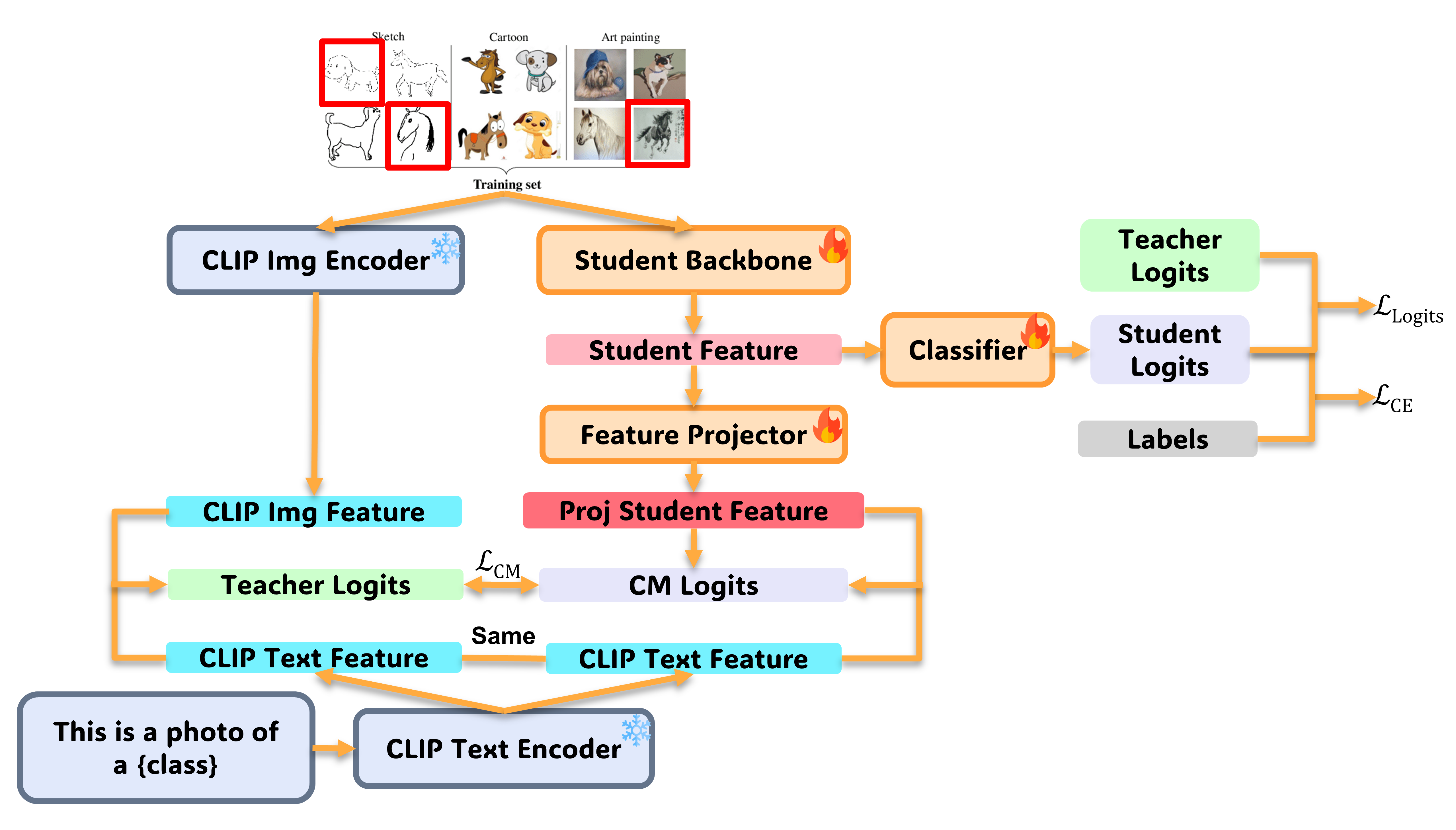
Figure 1: SCMD that features a selection mechanism to focus on hard-to-learn samples and a cross-modality module that projects the student’s feature into CLIP multimodal space for alignment.

In this section, we provide a detailed description of our Selective Cross-Modality Distillation Framework, which leverages a pretrained and freezed CLIP model [36] as the guiding teacher model.

3.1 Vanilla Knowledge Distillation

The vanilla knowledge distillation process is

$$\begin{gathered}\hat{\theta}_{\text{KD}}=\underset{\theta}{\arg\min}\sum_{(\mathbf{x}_{i},\mathbf{y}_{i})\in(\mathbf{X},\mathbf{Y})}\mathcal{L}(\phi(\mathbf{x}_{i}),f(\mathbf{x}_{i};\theta))\\ +\lambda_{1}\mathcal{H}(f(\mathbf{x}_{i};\theta),\mathbf{y})\\ +\lambda_{2}R(\phi,f,p,q,\mathbf{x}_{i},\mathbf{y}_{i})\end{gathered}$$ (1)

where $\phi$ is the teacher model, $f(\cdot;\theta)$ is the student model. $(\mathbf{X},\mathbf{Y})$ is the standard dataset that is used for training the student model. $\mathcal{L}$ is a generic distance function (can be the KL divergence between soft target distributions), $\mathcal{H}$ represents a generic loss function (usually cross-entropy loss), and $R$ is an arbitrary designed regularization. $p$ and $q$ correspond to certain layers or attention maps.

3.2 Selection Mechanism

$$S={\mathbf{x}_{i}:\mathbf{x}_{i}\in\mathbf{X},i\in I}\quad\text{where }I={i:\mathcal{H}(f(\mathbf{x}_{i}),\mathbf{y}_{i})\geq\tau}$$ (2)

In the preceding equation, $\mathbf{X}$ denotes the batch of samples, $\mathbf{x}_{i}$ an individual sample, and $\mathbf{y}_{i}$ its true label. The set $S$ consists of selected samples. The function $\mathcal{H}(f(\mathbf{x}_{i};\theta),\mathbf{y}_{i})$ computes the cross-entropy loss for the $i$-th sample, while $I$ contains indices of samples in the batch with a cross-entropy loss exceeding the threshold $\tau$.

Cross-entropy loss quantifies the divergence between the predicted probability distribution and the actual labels. High cross-entropy indicates challenging samples or model uncertainty. In our optimization, we use this loss to identify hard-to-learn samples. During each forward pass, samples with higher losses are selected for adjustment, a methodology also adopted in prior works [6, 62, 63, 64].

The uniqueness of our method lies not in the recognition of hard-to-learn samples but in its integration within knowledge distillation. By doing so, we harness the teacher model’s rich knowledge more efficiently, optimizing the student model’s learning. We delve into the theoretical underpinning of our selection mechanism in Section 4.

The “hard-to-learn” tag for the samples can change each iteration. However, to ensure holistic learning across the entire training dataset, we switch to full-batch training for the final $k\%$ of the training epochs.

3.3 Cross-Modality Module

Various feature-based knowledge distillations have been explored [45, 46, 47, 48, 49], however, direct alignment of classification features often presents challenges. To address this, we exploit the robust cross-modal alignment capabilities of the CLIP [36] model and employ a cross-modality distillation strategy.

In the context of our method, the student features are transformed into the CLIP’s [36] multimodal space using a linear projection. This is analogous to how CLIP projects its image features into a multimodal space to achieve alignment with text embeddings. This transformation bridges the semantic gap between the student model and the teacher model, facilitating a more effective knowledge-transfer process. After projection, we calculate the scaled pairwise cosine similarity with the text embeddings derived from the CLIP [36] model.

Our cross-modality loss is expressed as follows:

$$\begin{gathered}\mathcal{L}_{CM}=D_{\text{KL}}(p^{t}||(p^{s})^{\prime})\\ \text{where $p^{t}$ is the soft target distribution of CLIP and }\\ (p^{s})^{\prime}=\sigma(\gamma\cdot P(e(\mathbf{x}_{i};\theta_{e}))\cdot\mathbf{\phi_{\text{text}}};T=t)\end{gathered}$$ (3)

In this equation, $\gamma$ is a scale factor, which adjusts the magnitude of the projected student feature. $e$ represents the backbone of the student model. A linear projection $P$ is applied to the student feature $e(x_{i};\theta_{e})$, and $\phi_{\text{text}}$ represents the text embedding of CLIP. $\sigma$ is the softmax function parameterized by the distillation temperature $T$.

In order to generate unbiased text features using CLIP, we use a generic template: “this is a photo of a {class}”. This method helps us avoid incorporating any human prior knowledge about the dataset, ensuring that the feature generation process remains objective and is not influenced by any preconceived human understanding of the data.

During the inference phase, we omit the feature projector, relying solely on the student model’s backbone and its associated classifier for generating predictions.

3.4 SCMD

Figure 1 illustrates the overall framework of our proposed method.

The final training objective can be summarized as follows:

$$\begin{gathered}\hat{\theta}_{\text{SCMD}}=\underset{\theta}{\arg\min}\sum_{(\mathbf{x}_{i},\mathbf{y}_{i})\in(\mathbf{X},\mathbf{Y})}\lambda_{1}\mathcal{H}(f(\mathbf{x}_{i};\theta),\mathbf{y}_{i})\\ +\lambda_{2}\mathcal{L}_{\text{logits}}+\lambda_{3}\mathcal{L}_{\text{CM}}\\ \text{where }\mathcal{L}_{\text{logits}}=D_{\text{KL}}(p^{t}||p^{s})\\ \text{ and }\mathbf{x}_{i}\text{ and }\mathbf{y}_{i}\\ \text{are the selected samples and corresponding labels}\end{gathered}$$ (4)

4 Theoretical Evidence for Selection Strategy

To be consistent with the notation, we let $(\mathbf{X},\mathbf{Y})$ denote the standard data set and $(\mathbf{x}_{i},\mathbf{y}_{i})$ be one of the samples. We let $\mathbf{P}$ denote a distribution and $\mathcal{P}$ denote the distribution of distributions. We let $f(\cdot;\theta)$ denote the student model, $\phi$ denote the teacher model, and $r(\cdot)$ denote the risk. For convenience of notation, we allow $r(\cdot)$ to be parameterized by a distribution or by a dataset.

When $r(\cdot)$ is parameterized by a dataset, we have the empirical risk as

$$r\big{(}(\mathbf{X},\mathbf{Y})\big{)}=\dfrac{1}{n}\sum_{(\mathbf{x}_{i},\mathbf{y}_{i})\in(\mathbf{X},\mathbf{Y})}\mathcal{L}(f(\mathbf{x}_{i};\theta),\mathbf{y}_{i}),$$

where $\mathcal{L}$ is a generic loss function.

When $r(\cdot)$ is parameterized by a distribution, we have the expected risk as

$$r\big{(}\mathbf{P}\big{)}=\mathbb{E}_{(\mathbf{x}_{i},\mathbf{y}_{i})\sim\mathbf{P}}\mathcal{L}(f(\mathbf{x}_{i};\theta),\mathbf{y}_{i}),$$

For simplicity of discussion, we only use $r\big{(}\mathbf{P},\epsilon\big{)}$ to denote robustness performance when we do not need to specify how the test distribution deviates from the training distribution.

Assumption 1.

for any data pair $(\mathbf{x}_{i},\mathbf{y}_{i})$ studied in the context of this paper, there is a gold standard labeling function (albeit unknown) that $\mathbf{y}_{i}=f(\mathbf{x}_{i})$.

We believe this assumption is fundamental for numerous works studying the robustness behaviors of models with respect to feature perturbations, especially in the context of OOD robustness, where the test dataset is manually collected rather than generated by noise addition. Intuitively, this assumption stipulates that a musical piece recognized in the training phase must also be identified as the same piece in the testing phase, despite substantial shifts in the performance style or instrument used. In other words, these variations in representation, akin to distribution shifts in data, should not alter the fundamental recognition of the piece, preserving the semantics of the data.

Lemma 4.1.

Given Assumptions A1 such that there is a gold standard labeling function for source and target domains. For two arbitrary distributions $\mathbf{P}^{\prime}$ and $\mathbf{P}$,

$$r(\mathbf{P}^{\prime})\leq r(\mathbf{P})+tv(\mathbf{P}^{\prime},\mathbf{P})$$

where $tv$ denotes the total variation.

Proof. We leave the proof in Appendix A

Lemma 4.2.

Given the assumption that samples are independent and identically distributed, hypothesis space $\Theta$ and any $\delta>0$, with probability at least $1-\delta$, we have

$$r\big{(}\mathbf{P}^{\prime})\leq r\big{(}(\mathbf{X},\mathbf{Y})_{\mathbf{P}}\big{)}+tv(\mathbf{P}^{\prime},\mathbf{P})+\xi(n_{(\mathbf{X},\mathbf{Y})_{\mathbf{P}}},\Theta,\delta)$$

where we let $n_{(\mathbf{X},\mathbf{Y})_{\mathbf{P}}}$ denote the number of sample sizes in the finite dataset $(\mathbf{X},\mathbf{Y})_{\mathbf{P}}$, $\xi$ is a vanilla term that connects the number of samples and hypothesis space with generalization error bound.

Proof. We leave the proof in Appendix A

The above results demonstrates that empirical robustness is determined by three factors: the divergence between training and test distributions, the measurable empirical error on the training distribution, and a technical term influenced by sample size and hypothesis space. Therefore, the critical term that will bound the robustness performance is how the training distribution deviates from the testing distribution. This intuitively gives us the idea that training with the distributions that are the most similar to the test distribution will benefit the model most.

The above results apply to arbitrary distributions $\mathbf{P}\sim\mathcal{P}$. However, this does not necessarily encode the characteristics of the cases we are studying: some samples are hard for the model to learn.

To address this, we consider datasets generated by multiple distributions, some of which present more challenging learning scenarios. We represent these as a set $P$, consisting of m distributions, i.e., $P=\{\mathbf{P}_{1},\mathbf{P}_{2},\dots,\mathbf{P}_{m}\}$. Each data point is considered to be sampled from these distributions. For the convenience of discussion, we use $tv(\mathbf{P}^{\prime},P)$ to denote the average divergence between the distributions within the set. $tv(\mathbf{P}^{\prime},P):=\sum_{i}^{m}tv(\mathbf{P}^{\prime},\mathbf{P}_{i})/m,\forall\mathbf{P}_{i}\in P$.

Finally, we use $s()$ to denote the distribution selection mechanism, and compare two selection mechanisms: selecting the hard-to-learn samples (denoted as $s_{1}$) and selecting random samples (denoted as $s_{2}$).

Lemma 4.3.

$\mathcal{P}$ is continuous and has a finite expected value; for the two selection mechanism that are formally defined as

$$tv(s_{1}(P),P)=\sup_{\mathbf{P}\in P}tv(\mathbf{P},P),\quad\mathbb{E}_{\mathcal{P}}tv(s_{2}(P),P)=0$$

for a fixed testing dataset $\mathbf{P}^{\prime}$, with the assumption that $tv(P,\mathbf{P}^{\prime})=tv(P,\mathbf{P})+tv(\mathbf{P},\mathbf{P}^{\prime}),\forall\mathbf{P}\in P$ we have

$$\mathbb{E}_{\mathcal{P}}\Big{[}tv(s_{1}(P),\mathbf{P}^{\prime})\Big{]}\leq\mathbb{E}_{\mathcal{P}}\Big{[}tv(s_{2}(P),\mathbf{P}^{\prime})\Big{]}$$

Proof. We leave the proof in Appendix A

Our result compares the upper-bounded differences between the two training distribution selection strategies, and our results suggest that selecting the hard-to-learn samples will lead to a tighter generalization error bound.

Another important factor to note is that, given assumption A1 and Lemma 4.1 and 4.2, the selection strategy applicable to our theoretical discussion (i.e. $tv(s_{1}(P),P)=\sup_{\mathbf{P}\in P}tv(\mathbf{P},P)$) is only when selecting the hard-to-learn samples according to the label of the samples (thus cross-entropy loss). Other selection strategies such as selecting based on KL-divergence or distillation loss (experimented in Section 6.2) despite might following a similar goal, does not strictly match our theoretical discussion with will likely lead to an error bound in between $s_{1}$ and $s_{2}$. Therefore, with the support of the theoretical discussion, we argue that the most effective hard-to-learn selection mechanism is to be based on cross-entropy loss.

Another possible question is that the assumption $tv(P,\mathbf{P}^{\prime})=tv(P,\mathbf{P})+tv(\mathbf{P},\mathbf{P}^{\prime}),\forall\mathbf{P}\in P$ might appear strong. In fact, the proof will hold with any assumptions that describe the concept that the more different one distribution is from the average of the training set, the more it will benefit the testing distribution. In the typical domain generalization setting, where there are no guaranteed connections between training and testing distributions, we believe this is one of the practical assumptions we can consider, also widely used in practical by other domain generalization literature [6, 62, 63, 64].

5 Experiment

Algorithm	Ens/MA	VLCS	PACS	OffHome	TerraInc	DNet	Avg
Teacher (CLIP with ViT-B/32)	No	78.4 $\pm$ 0.0	94.7 $\pm$ 0.1	79.6 $\pm$ 0.1	19.0 $\pm$ 0.1	54.0 $\pm$ 0.0	65.1
ERM [8]	No	77.5 $\pm$ 0.4	85.5 $\pm$ 0.2	66.5 $\pm$ 0.3	46.1 $\pm$ 1.8	40.9 $\pm$ 0.1	63.3
CORAL [65]	No	78.8 $\pm$ 0.6	86.2 $\pm$ 0.3	68.7 $\pm$ 0.3	47.6 $\pm$ 1.0	41.5 $\pm$ 0.1	64.6
VREx [66]	No	78.3 $\pm$ 0.2	84.9 $\pm$ 0.6	66.4 $\pm$ 0.6	46.4 $\pm$ 0.6	33.6 $\pm$ 2.9	61.9
RSC [5]	No	77.1 $\pm$ 0.5	85.2 $\pm$ 0.9	65.5 $\pm$ 0.9	46.6 $\pm$ 1.0	38.9 $\pm$ 0.5	62.7
ERM + SWAD [30]	Yes	79.1 $\pm$ 0.1	88.1 $\pm$ 0.1	70.6 $\pm$ 0.2	50.0 $\pm$ 0.3	46.5 $\pm$ 0.1	66.9
CORAL + SWAD [30]	Yes	78.9 $\pm$ 0.1	88.3 $\pm$ 0.1	71.3 $\pm$ 0.1	51.0 $\pm$ 0.1	46.8 $\pm$ 0.0	67.3
AdaClust [67]	No	78.9 $\pm$ 0.6	87.0 $\pm$ 0.3	67.7 $\pm$ 0.5	48.1$\pm$ 0.1	43.3 $\pm$ 0.5	64.9
MIRO + SWAD [35]	Yes	79.6 $\pm$ 0.2	88.4 $\pm$ 0.1	72.4 $\pm$ 0.1	52.9 $\pm$ 0.2	47.0 $\pm$ 0.0	68.1
EoA [31]	Yes	79.1	88.6	72.5	52.3	47.4	68.0
Model ratatouille (Greedy)[68]	Yes	78.7 $\pm$ 0.2	90.5 $\pm$ 0.2	73.4 $\pm$ 0.3	49.2 $\pm$ 0.9	47.7 $\pm$ 0.0	67.9
Model ratatouille (Uniform)[68]	Yes	78.3	89.8	73.5	52.0	47.7	68.3
SCMD (ours)	Yes	80.9 $\pm$ 0.2	90.1 $\pm$ 0.0	74.8 $\pm$ 0.1	51.3 $\pm$ 0.2	48.4 $\pm$ 0.0	69.1

Table 1: Performance benchmarking on 5 datasets of the DomainBed benchmark. Gray background shows our proposed method. Experiments report the performance based on training-domain validation accuracy follow [7]. ‘Ens/MA’ stands for Ensemble/Moving Average. (best in bold and second underlined)

In this section, we demonstrate the effectiveness of our proposed method using the DomainBed [7] benchmark and compare it to the current state-of-the-art DG techniques.

5.1 Experimental Setup

We adhere to the protocol set out in [7] for our experimental setup and assess the performance of SCMD using VLCS [69], PACS [70], OfficeHome [71], TerraIncognita [72], and DomainNet [73]. It is noteworthy that CLIP does not perform well on the TerraIncognita [72] dataset, and we will explore these results in the discussion section.

Due to the intensive computing requirements of DomainBed’s [7] hyperparameter search protocol, we take a more simplified approach. We restrict our research to five distinct hyperparameter combinations, each tested three times. We assign 80% of the data for training and 20% for validation, choose the model based on the training-domain validation and report the results on the held-out domain.

In order to make a fair comparison with other methods, we use ResNet50 [74] as the student model and CLIP [36], with ViT-B/32 as its image encoder, as the teacher model, which is in line with existing research.

In line with the findings of previous studies [30, 31], we incorporate weight averaging into our experiments to access SCMD performance. This technique has been shown to mitigate the discrepancy between training-validation performance and out-of-domain test performance.

Eight RTX 3090 GPUs are utilized for all experiments.

5.2 Experimental results

We compare SCMD with other domain generalization algorithms on five datasets: PACS [70], VLCS [69], OfficeHome [71], TerraIncognita [72], and DomainNet [73]. We use ResNet50 pretrained on ImageNet1k [42] as the backbone. Table 1 shows that our proposed method achieves the best performance on the DomainBed benchmark for the ResNet50 model. It outperforms the existing methods on all datasets, with Model ratatouille [68] coming in second.

Model Ratatouille [68] utilizes a technique that adjusts the model on multiple extra tasks to obtain different weight initializations. These weights are then adjusted for the desired tasks, and the final model is created by taking the average of these weights. This is demonstrated by Model Ratatouille (Uniform) [68], which averages a total of 60 models to achieve the final result.

In contrast, our proposed method employs a teacher model and evaluates performance on a single model. Our method is orthogonal to existing DG methods, potentially providing additional avenues and perspectives in the broader landscape of DG research.

6 Ablation Studies

We carry out a thorough analysis of the SCMD algorithm by breaking it down into its components and examining them using the PACS dataset [70]. To ensure consistency and comparability with the main experiment, we use the same standardized hyperparameter search protocol.

We conduct a series of experiments on PACS [70] to evaluate the effectiveness of the proposed cross-modality module and the selection mechanism.

6.1 Impact of the Cross-Modality Module

Table 2 (Top Section) presents the comprehensive results of our method alongside its different variations.

• “Vanilla KD” [1] denotes the conventional knowledge distillation technique where the KL divergence between the predicted distributions of the student and teacher models is minimized.

• ‘SCMD (logits)” is the combination of the selection mechanism and the minimization of KL divergence.

• “SCMD (logits + CM)” represents the full version of our method, including all our proposed components.

We have included weight averaging [30, 31] into the Vanilla KD to guarantee a fair comparison and show the effectiveness of our proposed components. This technique has been previously demonstrated to enhance performance.

As shown in the top part of Table 2, our selection mechanism alone leads to a 0.5% improvement in comparison to the average performance of Vanilla KD. Additionally, our cross-modality module further boosts the performance by 0.6%. When both are combined, our proposed methodology offers a significant increase in performance, surpassing Vanilla KD by a total of 1.1%. These results demonstrate the combined power and effectiveness of our proposed approach.

Algorithm	Avg
SCMD (logits + CM) (full method)	90.1 $\pm$ 0.0
Vanilla KD [1]	89.0 $\pm$ 0.3
SCMD (logits)	89.5 $\pm$ 0.2
SCMD (selection based on CE loss)	90.1 $\pm$ 0.0
SCMD (selection based on KL)	89.6 $\pm$ 0.3
SCMD (selection based on distill loss)	89.8 $\pm$ 0.2
SCMD (no selection)	89.4 $\pm$ 0.3

Table 2: Performance evaluations: (Top) Impact of the cross-modality module in SCMD on the PACS dataset. (Bottom) SCMD performance with different strategies for selecting hard-to-learn samples on the PACS dataset. (best in bold)

6.2 Empirical Validation of Our Theoretical Analysis

As illustrated in Table 2 (Bottom Section), we employed various selection strategies for the samples.

• “selection based on KL” refers to sample selection based on the KL-divergence between the predicted distributions of the student and teacher models.

• “selection based on distill loss” implies that samples are chosen according to the distill loss, as defined in Eq 4.

• “no selection” represents the baseline scenario where the entire training dataset is used without any hard-to-learn sample selection.

• “selection based on CE loss” denotes our proposed selection strategy.

It is evident that any selection strategy yields better results than the “no selection” baseline. Our proposed “selection based on CE loss” approach is the most successful on the PACS dataset, outperforming “selection based on KL” by 0.5%, “selection based on distill loss” by 0.3%, and the no selection strategy by 0.7%. It is worth noting that the “distill loss” (Eq 4) includes the cross-entropy loss, which could explain why its performance is similar to “selection based on CE loss”, albeit slightly lower.

Prompt	Avg
this is an art of a {}	$88.9\pm 0.4$
this is a sketch of a {}	$89.6\pm 0.2$
this is a cartoon of a {}	$88.7\pm 0.4$
a photo of a {}	$89.9\pm 0.2$
this is a photo of a {}	$89.9\pm 0.4$
a {}	$88.8\pm 0.2$

Table 3: The performance of SCMD was tested on PACS with different prompts, using the same hyperparameters for three trials. The teacher model was Clip ViT-B/32 and the student model was RN50.

These results provide empirical support to our theoretical proposition: “Other selection strategies such as selecting based on KL-divergence or distillation loss despite might following a similar goal, do not strictly match our theoretical discussion which will likely lead to an error bound between $s_{1}$ and $s_{2}$.” Therefore, with the support of the theoretical discussion, we argue that the most effective hard-to-learn selection mechanism is to be based on cross-entropy loss.

7 Discussion and Limitations

7.1 Impact of Prompts Variations

In order to reduce bias in the feature extraction process with CLIP, we use a template that does not contain any human-derived insights, which is: “this is a photo of a {}”. This template anchors the feature generation process in a way that is not dependent on any particular domain, thus avoiding the impact of any human preconceptions.

Our experiments show that the prompt “photo” was the most effective for optimizing performance. We also found that slight changes to the prompt, such as “a photo of a {}” and “this is a photo of a {}”, had little effect on the success of the distillation process. This demonstrates the resilience of feature distillation to minor changes in the prompt structure. Table 3 provides further details on the ablation studies.

7.2 Analysis on TerraInc Performance

Table 4: Impact of KD on TerraIncognita. ‘MA’: Moving Average. ‘SCMD_no_KD’: variant when KD not used.

Algorithm	MA	Terra Avg
ERM	No	$46.1\pm 1.8$
SCMD	Yes	$51.3\pm 0.2$
SCMD-no-KD	Yes	$53.1\pm 0.5$

We observed suboptimal zero-shot performance from the CLIP model when we distilled it into ResNet50 using the TerraIncognita dataset, as shown in Table 1. Despite this, our approach still provided a benefit in the form of selective learning, as SCMD-no-KD outperformed ERM. This implies that preconditioning the CLIP model with fine-tuning before distillation may be a useful strategy to improve performance metrics for tasks like these.

7.3 Experiments on various student models

We investigate the effect of different teacher models and model sizes by exploring the applicability of our proposed method using the PACS dataset [70]. We use ResNet152 and ResNet18 [74] and follow the same experimental setup and hyperparameter search protocol as in our previous experiments.

Table 5 shows that SCMD outperforms Vanilla KD, even when different CLIP models are used as the teacher, such as RN101. In this case, SCMD achieved an improvement of approximately 0.6% compared to vanilla KD, which highlights the versatility of our approach and its effectiveness in both cross-architecture and homologous-architecture distillation scenarios.

Our approach yields a noteworthy improvement of 3.4% over the ERM [8] technique and 0.8% over Vanilla KD when distilled into ResNet152 [74]. Even with a smaller model such as ResNet18 [74], our method still shows strong performance compared to other DG methods, with a marginal improvement of only 0.2% over Vanilla KD. This slight difference may be due to the large capacity gap between ResNet18 [74] and CLIP [36].

Algorithm	CLIP	Student	Avg
ERM(reproduced)	ViT-B/32	/	94.7 $\pm$ 0.1
ERM(reproduced)	RN101	/	94.9 $\pm$ 0.1
SCMD	RN101	RN-50	88.5 $\pm$ 0.2
Vanilla KD			87.9 $\pm$ 0.3
ERM (reproduced)	ViT-B/32	RN-152	88.7 $\pm$ 0.5
SCMD			92.1 $\pm$ 0.2
Vanilla KD			91.3 $\pm$ 0.1
ERM [75]	ViT-B/32	RN-18	81.5 $\pm$ 0.0
RSC [5]			82.8 $\pm$ 0.4
IRM [76]			81.1 $\pm$ 0.3
MMD [10]			81.7 $\pm$ 0.2
SCMD			85.0 $\pm$ 0.2
Vanilla KD			84.8 $\pm$ 0.3

Table 5: Evaluation of SCMD’s performance across various student and CLIP model architectures on the PACS dataset

8 Conclusion

In this paper, we present Selective Cross-Modality Distillation (SCMD) for Domain Generalization, a novel approach that builds upon the existing knowledge distillation framework. Our method is designed to supplement existing DG techniques. We introduce a cross-modality module that leverages the robust cross-modal alignment capabilities of the CLIP model. The selection mechanism at the core of SCMD is supported by a thorough theoretical analysis and empirically validated through extensive experiments that demonstrate the efficacy of our proposed method.

Appendix A Theoretical Evidence for Selection Strategy

To be consistent with notation, we let $(\mathbf{X},\mathbf{Y})$ denote the standard dataset, and $(\mathbf{x}_{i},\mathbf{y}_{i})$ as one of the samples. We let $\mathbf{P}$ denote a distribution and $\mathcal{P}$ denote the distribution of distributions. We let $f(\cdot;\theta)$ denote the student model, $\phi$ denote the teacher model, and $r(\cdot)$ denote the risk. For the convenience of notations, we allow $r(\cdot)$ to be parameterized by a distribution or by a dataset.

Lemma A.1.

Given assumptions A1 such that there is a gold standard labeling function for source and target domains. For two arbitrary distributions $\mathbf{P}^{\prime}$ and $\mathbf{P}$,

$$r(\mathbf{P}^{\prime})\leq r(\mathbf{P})+tv(\mathbf{P}^{\prime},\mathbf{P})$$

where $tv$ denotes the total variation.

Proof.

Recall that we are assuming the same labelling function, let $\sigma$ and $\sigma^{\prime}$ be the density functions of $\mathbf{P}$ and $\mathbf{P}^{\prime}$

$$\begin{gathered}r(\mathbf{P}^{\prime})=r(\mathbf{P}^{\prime})+r(\mathbf{P})-r(\mathbf{P})\leq r(\mathbf{P})+\mid r(\mathbf{P}^{\prime})-r(\mathbf{P})\mid\\ \leq r(\mathbf{P})+\int\mid\sigma(\mathbf{x})-\sigma^{\prime}(\mathbf{x})\mid\mid f(\mathbf{x};\theta)-\mathbf{y}\mid d\mathbf{x}\\ \leq r(\mathbf{P})+tv(\mathbf{P}^{\prime},\mathbf{P})\end{gathered}$$

∎

Lemma A.2.

Given assumption that samples are independent and identically distributed, hypothesis space $\Theta$ and any $\delta>0$, with probability at least $1-\delta$, we have

$$r\big{(}\mathbf{P}^{\prime})\leq r\big{(}(\mathbf{X},\mathbf{Y})_{\mathbf{P}}\big{)}+tv(\mathbf{P}^{\prime},\mathbf{P})+\xi(n_{(\mathbf{X},\mathbf{Y})_{\mathbf{P}}},\Theta,\delta)$$

where we let $n_{(\mathbf{X},\mathbf{Y})_{\mathbf{P}}}$ denote the number of sample sizes in the finite dataset $(\mathbf{X},\mathbf{Y})_{\mathbf{P}}$, $\xi$ is a vanilla term that connects the number of samples and hypothesis space with generalization error bound.

Proof.

Recall that we are assuming that samples are independent and identically distributed, we have $\xi(n_{(\mathbf{X},\mathbf{Y})_{\mathbf{P}}},\Theta,\delta)=2\mathcal{R}(\mathcal{L})+\sqrt{(\log 1/\delta)/2n}$ where $\mathcal{R(\mathcal{L})}$ stands for Rademacher complexity and $\mathcal{L}=\{l_{\theta}\mid\theta\in\Theta\}$ where $l_{\theta}$ is the loss function corresponding to the student model $f(\cdot;\theta)$

$$\begin{gathered}r(\mathbf{P}^{\prime})=r(\mathbf{P})+tv(\mathbf{P}^{\prime},\mathbf{P})\\ \leq r\big{(}(\mathbf{X},\mathbf{Y})_{\mathbf{P}}\big{)}+tv(\mathbf{P}^{\prime},\mathbf{P})+\xi(n_{(\mathbf{X},\mathbf{Y})_{\mathbf{P}}},\Theta,\delta)\end{gathered}$$

This is an direct application of Theorem 1.1 and generalization error bound. ∎

The above results demonstrates that empirical robustness is determined by three factors: the divergence between training and test distributions, the measurable empirical error on the training distribution, and a technical term influenced by sample size and hypothesis space. Therefore, the critical term that will bound the robustness performance is how the training distribution deviates from the testing distribution. This intuitively give us the idea that training with the distributions that are the most similar to the test distribution will benefit the model most.

The above results apply to arbitrary distributions $\mathbf{P}\sim\mathcal{P}$. However, this does not necessarily encode the characteristics of the cases we are studying: some samples are hard for the model to learn.

To address this, we consider datasets generated by multiple distributions, some of which present more challenging learning scenarios. We represent these as a set $P$, consisting of m distributions, i.e., $P=\{\mathbf{P}_{1},\mathbf{P}_{2},\dots,\mathbf{P}_{m}\}$. Each data point is considered as sampled from these distributions. For the convenience of discussion, we use $tv(\mathbf{P}^{\prime},P)$ to denote the average divergence between the distributions within the set. $tv(\mathbf{P}^{\prime},P):=\sum_{i}^{m}tv(\mathbf{P}^{\prime},\mathbf{P}_{i})/m,\quad\forall\mathbf{P}_{i}\in P$.

Finally, we use $s()$ to denote the distribution selection mechanism, and we compare two selection mechanisms: selecting the hard-to-learn samples (denoted as $s_{1}$) and selecting random samples (denoted as $s_{2}$).

Lemma A.3.

$\mathcal{P}$ is continuous and has a finite expected value; for the two selection mechanism that are formally defined as

$$tv(s_{1}(P),P)=\sup_{\mathbf{P}\in P}tv(\mathbf{P},P),\quad\mathbb{E}_{\mathcal{P}}tv(s_{2}(P),P)=0$$

for a fixed testing dataset $\mathbf{P}^{\prime}$, with the assumption that $tv(P,\mathbf{P}^{\prime})=tv(P,\mathbf{P})+tv(\mathbf{P},\mathbf{P}^{\prime}),\forall\mathbf{P}\in P$ we have

$$\mathbb{E}_{\mathcal{P}}\Big{[}tv(s_{1}(P),\mathbf{P}^{\prime})\Big{]}\leq\mathbb{E}_{\mathcal{P}}\Big{[}tv(s_{2}(P),\mathbf{P}^{\prime})\Big{]}$$

Proof.

Based on our definition of $s_{1}$ and $s_{2}$,

$$\mathbb{E}_{\mathcal{P}}tv(s_{2}(P),\mathbf{P}^{\prime})=\mathbb{E}_{\mathcal{P}}tv(P,\mathbf{P}^{\prime})$$

And based on our assumption that $tv(P,\mathbf{P}^{\prime})=tv(P,\mathbf{P})+tv(\mathbf{P},\mathbf{P}^{\prime})$, we have

$$\begin{gathered}\mathbb{E}_{\mathcal{P}}\Big{[}tv(s_{1}(P),\mathbf{P}^{\prime})-tv(s_{2}(P),\mathbf{P}^{\prime})\Big{]}\\ =\mathbb{E}_{\mathcal{P}}\Big{[}\inf_{\mathbf{P}\in P}tv(\mathbf{P},\mathbf{P}^{\prime})-\mathbb{E}_{\mathcal{P}}tv(P,\mathbf{P}^{\prime})\Big{]}\leq 0\end{gathered}$$

∎

Our result compares the upper-bounded differences between the two training distribution selection strategies, and our results suggest that selecting the hard-to-learn samples will lead to a tighter generalization error bound.

Another important factor to note is that, given assumption A1 and Theorem 0.1, the selection strategy applicable to our theoretical discussion (i.e. $tv(s_{1}(P),P)=\sup_{\mathbf{P}\in P}tv(\mathbf{P},P)$) is only when selecting the hard-to-learn samples according to the label of the samples (thus, cross-entropy loss). Other selection strategies such as selecting based on KL-divergence or distillation loss despite might following a similar goal, do not strictly match our theoretical discussion, which will likely lead to an error bound in between $s_{1}$ and $s_{2}$. Therefore, with the support of the theoretical discussion, we argue that the most effective hard-to-learn selection mechanism is to be based on cross-entropy loss.

Another possible question is that Assumption $tv(P,\mathbf{P}^{\prime})=tv(P,\mathbf{P})+tv(\mathbf{P},\mathbf{P}^{\prime})$ might appear strong. In fact, the proof will hold with any assumptions that describe the concept that the more different one distribution is from the average of the training set, the more it will benefit the testing distribution. In the typical domain generalization setting, where there are no guaranteed connections between training and testing distributions, we believe this is one of the practical assumptions we can consider, also widely used in practical context by other domain generalization literature [6, 62, 63, 64]

Appendix B Method

B.1 Algorithm

Algorithm 1 Selective Cross-Modality Distillation

Input: Dataset $(\mathcal{X},\mathcal{Y})$ of size $n$; Percentile of hard-to-learn samples per batch $\rho$; Percentile of full-batch training $\kappa$; Batch size $\eta$; Maximum number of iterations $T$; Feature Projector $P$; pretrained teacher model $\phi$; Student model $\theta$ (randomly initialized)
Output: Trained student model $\theta$

  while t $\leq$ T do

     while t $\leq$ $(1-\kappa)T$ do

        Identify top $\rho$ percentile samples with highest Cross-entropy loss based on Eq 2

        For selected samples, compute student features and project to CLIP’s multi-modal space via $P$.

        Distill knowledge from the teacher model $\phi$ to the student model $\theta$ using Eq 4

     end while

     Distill knowledge from $\phi$ to $\theta$ across the entire batch and calculate the final loss with Eq 4

  end while

  return optimized student model $\theta$

B.2 Selection Mechanism

$$S={\mathbf{x}_{i}:\mathbf{x}_{i}\in\mathbf{X},i\in I}\quad\text{where }I={i:\mathcal{H}(f(\mathbf{x}_{i}),\mathbf{y}_{i})\geq\tau}$$ (5)

In the preceding equation, $\mathbf{X}$ denotes the batch of samples, $\mathbf{x}_{i}$ an individual sample, and $\mathbf{y}_{i}$ its true label. The set $S$ consists of selected samples. The function $\mathcal{H}(f(\mathbf{x}_{i};\theta),\mathbf{y}_{i})$ computes the cross-entropy loss for the $i$-th sample, while $I$ contains indices of samples in the batch with a cross-entropy loss exceeding the threshold $\tau$.

B.3 Cross-Modality Module

$$\begin{gathered}\mathcal{L}_{CM}=D_{\text{KL}}(p^{t}||(p^{s})^{\prime})\\ \text{where $p^{t}$ is the soft target distribution of CLIP and }\\ (p^{s})^{\prime}=\sigma(\gamma\cdot P(e(\mathbf{x}_{i};\theta_{e}))\cdot\mathbf{\phi_{\text{text}}};T=t)\end{gathered}$$ (6)

In this equation, $\gamma$ is a scale factor, which adjusts the magnitude of the projected student feature. $e$ represents the backbone of the student model. A linear projection $P$ is applied to the student feature $e(x_{i};\theta_{e})$, and $\phi_{\text{text}}$ represents the text embedding of CLIP. $\sigma$ is the softmax function parameterized by the distillation temperature $T$.

B.4 SCMD

$$\begin{gathered}\hat{\theta}_{\text{SCMD}}=\underset{\theta}{\arg\min}\sum_{(\mathbf{x}_{i},\mathbf{y}_{i})\in(\mathbf{X},\mathbf{Y})}\lambda_{1}\mathcal{H}(f(\mathbf{x}_{i};\theta),\mathbf{y}_{i})\\ +\lambda_{2}\mathcal{L}_{\text{logits}}+\lambda_{3}\mathcal{L}_{\text{CM}}\\ \text{where }\mathcal{L}_{\text{logits}}=D_{\text{KL}}(p^{t}||p^{s})\\ \text{ and }\mathbf{x}_{i}\text{ and }\mathbf{y}_{i}\\ \text{are the selected samples and their corresponding labels}\end{gathered}$$ (7)

Appendix C Compare with other KD methods

Algorithm	MA	Avg
FitNet [77]	Yes	$88.4\pm 0.2$
BSS [78]	Yes	$89.3\pm 0.1$
RKD [79]	Yes	$87.4\pm 0.2$
Vanilla [1]	Yes	$89.0\pm 0.3$
SCMD	Yes	$90.1\pm 0.0$

Table 6: SCMD vs. other KD on PACS. “MA”: Moving Average

At the core of SCMD is the knowledge distillation process, which is essential to its design. To evaluate the effectiveness of SCMD, we conducted comparative experiments with other knowledge distillation methods on the PACS dataset. The results in Table 6 demonstrate that SCMD outperforms these contemporary techniques.

Appendix D Full Results

The full details of the results presented in Table 1 of the main paper are displayed in Table 7.

Table 7: Detailed Performance of SCMD and Vanilla KD

VLCS
	CLIP	Student	A	C	P	S	Avg
SCMD	ViT-B/32	RN50	98.8 $\pm$ 0.1	64.6 $\pm$ 0.4	78.2 $\pm$ 0.3	81.9 $\pm$ 0.3	80.9 $\pm$ 0.2
PACS
			C	L	S	V	Avg
SCMD	ViT-B/32	RN50	92.9 $\pm$ 0.3	86.0 $\pm$ 0.3	99.0 $\pm$ 0.1	82.3 $\pm$ 0.1	90.1 $\pm$ 0.0
SCMD	ViT-B/32	RN152	94.0 $\pm$ 0.2	89.1 $\pm$ 0.5	99.3 $\pm$ 0.1	85.9 $\pm$ 0.6	92.1 $\pm$ 0.2
SCMD	ViT-B/32	RN18	84.7 $\pm$ 0.1	80.7 $\pm$ 0.5	96.2 $\pm$ 0.1	78.6 $\pm$ 0.6	85.0 $\pm$ 0.2
SCMD	RN101	RN50	90.2 $\pm$ 0.8	83.4 $\pm$ 0.3	99.1 $\pm$ 0.1	81.1 $\pm$ 0.8	88.5 $\pm$ 0.2
Vanilla KD	ViT-B/32	RN50	91.2 $\pm$ 0.2	85.2 $\pm$ 0.3	99.4 $\pm$ 0.1	80.3 $\pm$ 0.9	89.0 $\pm$ 0.3
Vanilla KD	ViT-B/32	RN152	93.8 $\pm$ 0.1	87.3 $\pm$ 0.4	99.6 $\pm$ 0.0	84.7 $\pm$ 0.2	91.3 $\pm$ 0.1
Vanilla KD	ViT-B/32	RN18	84.1 $\pm$ 0.5	80.0 $\pm$ 0.2	96.7 $\pm$ 0.2	78.5 $\pm$ 0.6	84.8 $\pm$ 0.3
Vanilla KD	RN101	RN50	89.8 $\pm$ 0.2	80.8 $\pm$ 0.9	99.1 $\pm$ 0.1	81.8 $\pm$ 0.5	87.9 $\pm$ 0.3
OfficeHome
			A	C	P	R	Avg
SCMD	ViT-B/32	RN50	72.7 $\pm$ 0.0	58.7 $\pm$ 0.1	82.4 $\pm$ 0.1	85.5 $\pm$ 0.1	74.8 $\pm$ 0.1
TerraIncognita
			L100	L38	L43	L46	Avg
SCMD	ViT-B/32	RN50	52.9 $\pm$ 1.1	45.3 $\pm$ 0.1	60.5 $\pm$ 0.5	46.6 $\pm$ 1.0	51.3 $\pm$ 0.2
DomainNet
			clip	info	paint	quick	real	sketch	Avg
SCMD	ViT-B/32	RN50	66.2 $\pm$ 0.1	25.2 $\pm$ 0.0	56.9 $\pm$ 0.2	14.3 $\pm$ 0.2	70.4 $\pm$ 0.0	57.4 $\pm$ 0.1	48.4 $\pm$ 0.0

D.1 hyperparameters search space

We adhere to the experimental setup described in the DomainBed [7] paper. The specifics of our setup are outlined below:

1. Data Split: We partition datasets into 80% training and 20% validation sets. Model selections are based on training domain validation performances, and we report on the corresponding test domain.

2. hyperparameters: Although many hyperparameters follow [7], deviations are documented in Table 8.

3. Batch & Decay: We adjust our batch size and weight decay following the guidelines of [30].

4. Dropout: The ResNet dropout rate is set to 0 to mitigate excessive randomness.

5. Learning Rate: We abandon the rate of $1\times 10^{-5}$ because it converges too slowly, and instead focus on rates of $3\times 10^{-5}$ and $5\times 10^{-5}$.

Table 9 presents the search space specific to our algorithm’s hyperparameters. While we consistently set $\lambda_{1}$, the balance factor for Cross-entropy, to 1, we perform random sweeps for the remaining weight factors.

Table 8: Unconditional hyperparameter search space. (U and list indicate Uniform distribution and random choice, respectively)

Parameter	Default Value	DomainBed [7]	SWAD [30]	Ours
batchsize	32	$2^{U(3,5.5)}$	32	32
learning rate	5e-5	$10^{U(-5,-3.5)}$	[1e-5, 3e-5, 5e-5]	[3e-5, 5e-5]
ResNet dropout	0	[0.0, 0.1, 0.5]	[0.0, 0.1, 0.5]	0
weight decay	0	$10^{U(-6,-2)}$	[1e-4, 1e-6]	[1e-4, 1e-6]

Table 9: Algorithm-specific hyperparameter search space. (U and list indicate Uniform distribution and random choice, respectively)

Parameter Default Value Sweep range $\lambda_{1}$ (for CE loss) 1 1 $\lambda_{2}$ 0.5 $U(0.5,1.0)$ $\lambda_{3}$ 0.5 $U(0.5,1.0)$ last_k_epoch 0.25 $U(0.2,0.4)$ Hard-to-learn sample percentage 1/3 $[0.2,0.25,0.3]$ temperature 3.0 $U(2.0,5.0)$

References

- [1] Geoffrey Hinton, Oriol Vinyals, and Jeff Dean. Distilling the knowledge in a neural network. ArXiv preprint, abs/1503.02531, 2015.
- [2] Shai Ben-David, John Blitzer, Koby Crammer, Alex Kulesza, Fernando Pereira, and Jennifer Wortman Vaughan. A theory of learning from different domains. Machine learning, 79:151–175, 2010.
- [3] Shai Ben-David, John Blitzer, Koby Crammer, and Fernando Pereira. Analysis of representations for domain adaptation. In Bernhard Schölkopf, John C. Platt, and Thomas Hofmann, editors, Advances in Neural Information Processing Systems 19, Proceedings of the Twentieth Annual Conference on Neural Information Processing Systems, Vancouver, British Columbia, Canada, December 4-7, 2006, pages 137–144. MIT Press, 2006.
- [4] Wang Lu, Jindong Wang, Haoliang Li, Yiqiang Chen, and Xing Xie. Domain-invariant feature exploration for domain generalization. ArXiv preprint, abs/2207.12020, 2022.
- [5] Zeyi Huang, Haohan Wang, Eric P Xing, and Dong Huang. Self-challenging improves cross-domain generalization. In Computer Vision–ECCV 2020: 16th European Conference, Glasgow, UK, August 23–28, 2020, Proceedings, Part II 16, pages 124–140. Springer, 2020.
- [6] Zeyi Huang, Haohan Wang, Dong Huang, Yong Jae Lee, and Eric P Xing. The two dimensions of worst-case training and the integrated effect for out-of-domain generalization. ArXiv preprint, abs/2204.04384, 2022.
- [7] Ishaan Gulrajani and David Lopez-Paz. In search of lost domain generalization. In 9th International Conference on Learning Representations, ICLR 2021, Virtual Event, Austria, May 3-7, 2021. OpenReview.net, 2021.
- [8] Vladimir N. Vapnik. Statistical Learning Theory. Wiley-Interscience, 1998.
- [9] Krikamol Muandet, David Balduzzi, and Bernhard Schölkopf. Domain generalization via invariant feature representation. In Proceedings of the 30th International Conference on Machine Learning, ICML 2013, Atlanta, GA, USA, 16-21 June 2013, volume 28 of JMLR Workshop and Conference Proceedings, pages 10–18. JMLR.org, 2013.
- [10] Haoliang Li, Sinno Jialin Pan, Shiqi Wang, and Alex C. Kot. Domain generalization with adversarial feature learning. In 2018 IEEE Conference on Computer Vision and Pattern Recognition, CVPR 2018, Salt Lake City, UT, USA, June 18-22, 2018, pages 5400–5409. IEEE Computer Society, 2018.
- [11] Ya Li, Xinmei Tian, Mingming Gong, Yajing Liu, Tongliang Liu, Kun Zhang, and Dacheng Tao. Deep domain generalization via conditional invariant adversarial networks. In Proceedings of the European conference on computer vision (ECCV), pages 624–639, 2018.
- [12] Haohan Wang, Aaksha Meghawat, Louis-Philippe Morency, and Eric P Xing. Select-additive learning: Improving generalization in multimodal sentiment analysis. In 2017 IEEE International Conference on Multimedia and Expo (ICME), pages 949–954. IEEE, 2017.
- [13] Kei Akuzawa, Yusuke Iwasawa, and Yutaka Matsuo. Adversarial invariant feature learning with accuracy constraint for domain generalization. In Machine Learning and Knowledge Discovery in Databases: European Conference, ECML PKDD 2019, Würzburg, Germany, September 16–20, 2019, Proceedings, Part II, pages 315–331. Springer, 2020.
- [14] Yu Ding, Lei Wang, Bin Liang, Shuming Liang, Yang Wang, and Fang Chen. Domain generalization by learning and removing domain-specific features. ArXiv preprint, abs/2212.07101, 2022.
- [15] Beining Han, Chongyi Zheng, Harris Chan, Keiran Paster, Michael R. Zhang, and Jimmy Ba. Learning domain invariant representations in goal-conditioned block mdps. In Marc’Aurelio Ranzato, Alina Beygelzimer, Yann N. Dauphin, Percy Liang, and Jennifer Wortman Vaughan, editors, Advances in Neural Information Processing Systems 34: Annual Conference on Neural Information Processing Systems 2021, NeurIPS 2021, December 6-14, 2021, virtual, pages 764–776, 2021.
- [16] Ruoyu Wang, Mingyang Yi, Zhitang Chen, and Shengyu Zhu. Out-of-distribution generalization with causal invariant transformations. In IEEE/CVF Conference on Computer Vision and Pattern Recognition, CVPR 2022, New Orleans, LA, USA, June 18-24, 2022, pages 375–385. IEEE, 2022.
- [17] Rang Meng, Xianfeng Li, Weijie Chen, Shicai Yang, Jie Song, Xinchao Wang, Lei Zhang, Mingli Song, Di Xie, and Shiliang Pu. Attention diversification for domain generalization. In Computer Vision–ECCV 2022: 17th European Conference, Tel Aviv, Israel, October 23–27, 2022, Proceedings, Part XXXIV, pages 322–340. Springer, 2022.
- [18] Kyungmoon Lee, Sungyeon Kim, and Suha Kwak. Cross-domain ensemble distillation for domain generalization. In Computer Vision–ECCV 2022: 17th European Conference, Tel Aviv, Israel, October 23–27, 2022, Proceedings, Part XXV, pages 1–20. Springer, 2022.
- [19] Songwei Ge, Haohan Wang, Amir Alavi, Eric Xing, and Ziv Bar-Joseph. Supervised adversarial alignment of single-cell rna-seq data. Journal of Computational Biology, 28(5):501–513, 2021.
- [20] Shiv Shankar, Vihari Piratla, Soumen Chakrabarti, Siddhartha Chaudhuri, Preethi Jyothi, and Sunita Sarawagi. Generalizing across domains via cross-gradient training. In 6th International Conference on Learning Representations, ICLR 2018, Vancouver, BC, Canada, April 30 - May 3, 2018, Conference Track Proceedings. OpenReview.net, 2018.
- [21] Xiangyu Yue, Yang Zhang, Sicheng Zhao, Alberto L. Sangiovanni-Vincentelli, Kurt Keutzer, and Boqing Gong. Domain randomization and pyramid consistency: Simulation-to-real generalization without accessing target domain data. In 2019 IEEE/CVF International Conference on Computer Vision, ICCV 2019, Seoul, Korea (South), October 27 - November 2, 2019, pages 2100–2110. IEEE, 2019.
- [22] Rui Gong, Wen Li, Yuhua Chen, and Luc Van Gool. DLOW: domain flow for adaptation and generalization. In IEEE Conference on Computer Vision and Pattern Recognition, CVPR 2019, Long Beach, CA, USA, June 16-20, 2019, pages 2477–2486. Computer Vision Foundation / IEEE, 2019.
- [23] Kaiyang Zhou, Yongxin Yang, Timothy M. Hospedales, and Tao Xiang. Deep domain-adversarial image generation for domain generalisation. In The Thirty-Fourth AAAI Conference on Artificial Intelligence, AAAI 2020, The Thirty-Second Innovative Applications of Artificial Intelligence Conference, IAAI 2020, The Tenth AAAI Symposium on Educational Advances in Artificial Intelligence, EAAI 2020, New York, NY, USA, February 7-12, 2020, pages 13025–13032. AAAI Press, 2020.
- [24] Jiaxing Huang, Dayan Guan, Aoran Xiao, and Shijian Lu. FSDR: frequency space domain randomization for domain generalization. In IEEE Conference on Computer Vision and Pattern Recognition, CVPR 2021, virtual, June 19-25, 2021, pages 6891–6902. Computer Vision Foundation / IEEE, 2021.
- [25] Zhuo Wang, Zezheng Wang, Zitong Yu, Weihong Deng, Jiahong Li, Tingting Gao, and Zhongyuan Wang. Domain generalization via shuffled style assembly for face anti-spoofing. In Proceedings of the IEEE/CVF Conference on Computer Vision and Pattern Recognition, pages 4123–4133, 2022.
- [26] Jindong Wang, Cuiling Lan, Chang Liu, Yidong Ouyang, Tao Qin, Wang Lu, Yiqiang Chen, Wenjun Zeng, and Philip Yu. Generalizing to unseen domains: A survey on domain generalization. IEEE Transactions on Knowledge and Data Engineering, 2022.
- [27] Muhammad Ghifary, W. Bastiaan Kleijn, Mengjie Zhang, and David Balduzzi. Domain generalization for object recognition with multi-task autoencoders. In 2015 IEEE International Conference on Computer Vision, ICCV 2015, Santiago, Chile, December 7-13, 2015, pages 2551–2559. IEEE Computer Society, 2015.
- [28] Yaroslav Ganin and Victor S. Lempitsky. Unsupervised domain adaptation by backpropagation. In Francis R. Bach and David M. Blei, editors, Proceedings of the 32nd International Conference on Machine Learning, ICML 2015, Lille, France, 6-11 July 2015, volume 37 of JMLR Workshop and Conference Proceedings, pages 1180–1189. JMLR.org, 2015.
- [29] Da Li, Yongxin Yang, Yi-Zhe Song, and Timothy M. Hospedales. Learning to generalize: Meta-learning for domain generalization. In Sheila A. McIlraith and Kilian Q. Weinberger, editors, Proceedings of the Thirty-Second AAAI Conference on Artificial Intelligence, (AAAI-18), the 30th innovative Applications of Artificial Intelligence (IAAI-18), and the 8th AAAI Symposium on Educational Advances in Artificial Intelligence (EAAI-18), New Orleans, Louisiana, USA, February 2-7, 2018, pages 3490–3497. AAAI Press, 2018.
- [30] Junbum Cha, Sanghyuk Chun, Kyungjae Lee, Han-Cheol Cho, Seunghyun Park, Yunsung Lee, and Sungrae Park. SWAD: domain generalization by seeking flat minima. In Marc’Aurelio Ranzato, Alina Beygelzimer, Yann N. Dauphin, Percy Liang, and Jennifer Wortman Vaughan, editors, Advances in Neural Information Processing Systems 34: Annual Conference on Neural Information Processing Systems 2021, NeurIPS 2021, December 6-14, 2021, virtual, pages 22405–22418, 2021.
- [31] Devansh Arpit, Huan Wang, Yingbo Zhou, and Caiming Xiong. Ensemble of averages: Improving model selection and boosting performance in domain generalization. Advances in Neural Information Processing Systems, 35:8265–8277, 2022.
- [32] Xin Zhang, Shixiang Shane Gu, Yutaka Matsuo, and Yusuke Iwasawa. Domain prompt learning for efficiently adapting clip to unseen domains. arXiv e-prints, pages arXiv–2111, 2021.
- [33] Kaiyang Zhou, Jingkang Yang, Chen Change Loy, and Ziwei Liu. Learning to prompt for vision-language models. International Journal of Computer Vision, 130(9):2337–2348, 2022.
- [34] Ziyue Li, Kan Ren, Xinyang Jiang, Bo Li, Haipeng Zhang, and Dongsheng Li. Domain generalization using pretrained models without fine-tuning. ArXiv preprint, abs/2203.04600, 2022.
- [35] Junbum Cha, Kyungjae Lee, Sungrae Park, and Sanghyuk Chun. Domain generalization by mutual-information regularization with pre-trained models. In Computer Vision–ECCV 2022: 17th European Conference, Tel Aviv, Israel, October 23–27, 2022, Proceedings, Part XXIII, pages 440–457. Springer, 2022.
- [36] Alec Radford, Jong Wook Kim, Chris Hallacy, Aditya Ramesh, Gabriel Goh, Sandhini Agarwal, Girish Sastry, Amanda Askell, Pamela Mishkin, Jack Clark, Gretchen Krueger, and Ilya Sutskever. Learning transferable visual models from natural language supervision. In Marina Meila and Tong Zhang, editors, Proceedings of the 38th International Conference on Machine Learning, ICML 2021, 18-24 July 2021, Virtual Event, volume 139 of Proceedings of Machine Learning Research, pages 8748–8763. PMLR, 2021.
- [37] Chao Jia, Yinfei Yang, Ye Xia, Yi-Ting Chen, Zarana Parekh, Hieu Pham, Quoc V. Le, Yun-Hsuan Sung, Zhen Li, and Tom Duerig. Scaling up visual and vision-language representation learning with noisy text supervision. In Marina Meila and Tong Zhang, editors, Proceedings of the 38th International Conference on Machine Learning, ICML 2021, 18-24 July 2021, Virtual Event, volume 139 of Proceedings of Machine Learning Research, pages 4904–4916. PMLR, 2021.
- [38] Jinyu Yang, Jiali Duan, Son Tran, Yi Xu, Sampath Chanda, Liqun Chen, Belinda Zeng, Trishul Chilimbi, and Junzhou Huang. Vision-language pre-training with triple contrastive learning. In Proceedings of the IEEE/CVF Conference on Computer Vision and Pattern Recognition, pages 15671–15680, 2022.
- [39] Jianwei Yang, Chunyuan Li, Pengchuan Zhang, Bin Xiao, Ce Liu, Lu Yuan, and Jianfeng Gao. Unified contrastive learning in image-text-label space. In Proceedings of the IEEE/CVF Conference on Computer Vision and Pattern Recognition, pages 19163–19173, 2022.
- [40] Lewei Yao, Runhui Huang, Lu Hou, Guansong Lu, Minzhe Niu, Hang Xu, Xiaodan Liang, Zhenguo Li, Xin Jiang, and Chunjing Xu. FILIP: fine-grained interactive language-image pre-training. In The Tenth International Conference on Learning Representations, ICLR 2022, Virtual Event, April 25-29, 2022. OpenReview.net, 2022.
- [41] Haoxuan You, Luowei Zhou, Bin Xiao, Noel Codella, Yu Cheng, Ruochen Xu, Shih-Fu Chang, and Lu Yuan. Learning visual representation from modality-shared contrastive language-image pre-training. In Computer Vision–ECCV 2022: 17th European Conference, Tel Aviv, Israel, October 23–27, 2022, Proceedings, Part XXVII, pages 69–87. Springer, 2022.
- [42] Jia Deng, Wei Dong, Richard Socher, Li-Jia Li, Kai Li, and Fei-Fei Li. Imagenet: A large-scale hierarchical image database. In 2009 IEEE Computer Society Conference on Computer Vision and Pattern Recognition (CVPR 2009), 20-25 June 2009, Miami, Florida, USA, pages 248–255. IEEE Computer Society, 2009.
- [43] Yu Cheng, Duo Wang, Pan Zhou, and Tao Zhang. A survey of model compression and acceleration for deep neural networks. ArXiv preprint, abs/1710.09282, 2017.
- [44] Chuanqi Tan, Fuchun Sun, Tao Kong, Wenchang Zhang, Chao Yang, and Chunfang Liu. A survey on deep transfer learning. In Artificial Neural Networks and Machine Learning–ICANN 2018: 27th International Conference on Artificial Neural Networks, Rhodes, Greece, October 4-7, 2018, Proceedings, Part III 27, pages 270–279. Springer, 2018.
- [45] Adriana Romero, Nicolas Ballas, Samira Ebrahimi Kahou, Antoine Chassang, Carlo Gatta, and Yoshua Bengio. Fitnets: Hints for thin deep nets. In Yoshua Bengio and Yann LeCun, editors, 3rd International Conference on Learning Representations, ICLR 2015, San Diego, CA, USA, May 7-9, 2015, Conference Track Proceedings, 2015.
- [46] Yoshua Bengio, Aaron Courville, and Pascal Vincent. Representation learning: A review and new perspectives. IEEE transactions on pattern analysis and machine intelligence, 35(8):1798–1828, 2013.
- [47] Sergey Zagoruyko and Nikos Komodakis. Paying more attention to attention: Improving the performance of convolutional neural networks via attention transfer. In 5th International Conference on Learning Representations, ICLR 2017, Toulon, France, April 24-26, 2017, Conference Track Proceedings. OpenReview.net, 2017.
- [48] Jangho Kim, Seonguk Park, and Nojun Kwak. Paraphrasing complex network: Network compression via factor transfer. In Samy Bengio, Hanna M. Wallach, Hugo Larochelle, Kristen Grauman, Nicolò Cesa-Bianchi, and Roman Garnett, editors, Advances in Neural Information Processing Systems 31: Annual Conference on Neural Information Processing Systems 2018, NeurIPS 2018, December 3-8, 2018, Montréal, Canada, pages 2765–2774, 2018.
- [49] Byeongho Heo, Jeesoo Kim, Sangdoo Yun, Hyojin Park, Nojun Kwak, and Jin Young Choi. A comprehensive overhaul of feature distillation. In 2019 IEEE/CVF International Conference on Computer Vision, ICCV 2019, Seoul, Korea (South), October 27 - November 2, 2019, pages 1921–1930. IEEE, 2019.
- [50] Ying Zhang, Tao Xiang, Timothy M. Hospedales, and Huchuan Lu. Deep mutual learning. In 2018 IEEE Conference on Computer Vision and Pattern Recognition, CVPR 2018, Salt Lake City, UT, USA, June 18-22, 2018, pages 4320–4328. IEEE Computer Society, 2018.
- [51] Jangho Kim, Seonguk Park, and Nojun Kwak. Paraphrasing complex network: Network compression via factor transfer. In Samy Bengio, Hanna M. Wallach, Hugo Larochelle, Kristen Grauman, Nicolò Cesa-Bianchi, and Roman Garnett, editors, Advances in Neural Information Processing Systems 31: Annual Conference on Neural Information Processing Systems 2018, NeurIPS 2018, December 3-8, 2018, Montréal, Canada, pages 2765–2774, 2018.
- [52] Hanting Chen, Yunhe Wang, Chang Xu, Chao Xu, and Dacheng Tao. Learning student networks via feature embedding. IEEE Transactions on Neural Networks and Learning Systems, 32(1):25–35, 2020.
- [53] Peyman Passban, Yimeng Wu, Mehdi Rezagholizadeh, and Qun Liu. ALP-KD: attention-based layer projection for knowledge distillation. In Thirty-Fifth AAAI Conference on Artificial Intelligence, AAAI 2021, Thirty-Third Conference on Innovative Applications of Artificial Intelligence, IAAI 2021, The Eleventh Symposium on Educational Advances in Artificial Intelligence, EAAI 2021, Virtual Event, February 2-9, 2021, pages 13657–13665. AAAI Press, 2021.
- [54] Xiaobo Wang, Tianyu Fu, Shengcai Liao, Shuo Wang, Zhen Lei, and Tao Mei. Exclusivity-consistency regularized knowledge distillation for face recognition. In Computer Vision–ECCV 2020: 16th European Conference, Glasgow, UK, August 23–28, 2020, Proceedings, Part XXIV 16, pages 325–342. Springer, 2020.
- [55] Zehao Huang and Naiyan Wang. Like what you like: Knowledge distill via neuron selectivity transfer. ArXiv preprint, abs/1707.01219, 2017.
- [56] Yuntao Chen, Naiyan Wang, and Zhaoxiang Zhang. Darkrank: Accelerating deep metric learning via cross sample similarities transfer. In Sheila A. McIlraith and Kilian Q. Weinberger, editors, Proceedings of the Thirty-Second AAAI Conference on Artificial Intelligence, (AAAI-18), the 30th innovative Applications of Artificial Intelligence (IAAI-18), and the 8th AAAI Symposium on Educational Advances in Artificial Intelligence (EAAI-18), New Orleans, Louisiana, USA, February 2-7, 2018, pages 2852–2859. AAAI Press, 2018.
- [57] Nikolaos Passalis, Maria Tzelepi, and Anastasios Tefas. Heterogeneous knowledge distillation using information flow modeling. In 2020 IEEE/CVF Conference on Computer Vision and Pattern Recognition, CVPR 2020, Seattle, WA, USA, June 13-19, 2020, pages 2336–2345. IEEE, 2020.
- [58] Nikolaos Passalis, Maria Tzelepi, and Anastasios Tefas. Probabilistic knowledge transfer for lightweight deep representation learning. IEEE Transactions on Neural Networks and Learning Systems, 32(5):2030–2039, 2020.
- [59] Kunran Xu, Lai Rui, Yishi Li, and Lin Gu. Feature normalized knowledge distillation for image classification. In Computer Vision–ECCV 2020: 16th European Conference, Glasgow, UK, August 23–28, 2020, Proceedings, Part XXV 16, pages 664–680. Springer, 2020.
- [60] Junjie Liu, Dongchao Wen, Hongxing Gao, Wei Tao, Tse-Wei Chen, Kinya Osa, and Masami Kato. Knowledge representing: efficient, sparse representation of prior knowledge for knowledge distillation. In Proceedings of the IEEE/CVF Conference on Computer Vision and Pattern Recognition Workshops, pages 0–0, 2019.
- [61] Yufan Liu, Jiajiong Cao, Bing Li, Weiming Hu, Jingting Ding, and Liang Li. Cross-architecture knowledge distillation. In Proceedings of the Asian Conference on Computer Vision, pages 3396–3411, 2022.
- [62] Jonathon Byrd and Zachary Chase Lipton. What is the effect of importance weighting in deep learning? In Kamalika Chaudhuri and Ruslan Salakhutdinov, editors, Proceedings of the 36th International Conference on Machine Learning, ICML 2019, 9-15 June 2019, Long Beach, California, USA, volume 97 of Proceedings of Machine Learning Research, pages 872–881. PMLR, 2019.
- [63] Haw-Shiuan Chang, Erik G. Learned-Miller, and Andrew McCallum. Active bias: Training more accurate neural networks by emphasizing high variance samples. In Isabelle Guyon, Ulrike von Luxburg, Samy Bengio, Hanna M. Wallach, Rob Fergus, S. V. N. Vishwanathan, and Roman Garnett, editors, Advances in Neural Information Processing Systems 30: Annual Conference on Neural Information Processing Systems 2017, December 4-9, 2017, Long Beach, CA, USA, pages 1002–1012, 2017.
- [64] Angelos Katharopoulos and François Fleuret. Not all samples are created equal: Deep learning with importance sampling. In Jennifer G. Dy and Andreas Krause, editors, Proceedings of the 35th International Conference on Machine Learning, ICML 2018, Stockholmsmässan, Stockholm, Sweden, July 10-15, 2018, volume 80 of Proceedings of Machine Learning Research, pages 2530–2539. PMLR, 2018.
- [65] Baochen Sun and Kate Saenko. Deep coral: Correlation alignment for deep domain adaptation. In Computer Vision–ECCV 2016 Workshops: Amsterdam, The Netherlands, October 8-10 and 15-16, 2016, Proceedings, Part III 14, pages 443–450. Springer, 2016.
- [66] David Krueger, Ethan Caballero, Jörn-Henrik Jacobsen, Amy Zhang, Jonathan Binas, Dinghuai Zhang, Rémi Le Priol, and Aaron C. Courville. Out-of-distribution generalization via risk extrapolation (rex). In Marina Meila and Tong Zhang, editors, Proceedings of the 38th International Conference on Machine Learning, ICML 2021, 18-24 July 2021, Virtual Event, volume 139 of Proceedings of Machine Learning Research, pages 5815–5826. PMLR, 2021.
- [67] Xavier Thomas, Dhruv Mahajan, Alex Pentland, and Abhimanyu Dubey. Adaptive methods for aggregated domain generalization. ArXiv preprint, abs/2112.04766, 2021.
- [68] Alexandre Ramé, Kartik Ahuja, Jianyu Zhang, Matthieu Cord, Léon Bottou, and David Lopez-Paz. Recycling diverse models for out-of-distribution generalization. ArXiv preprint, abs/2212.10445, 2022.
- [69] Chen Fang, Ye Xu, and Daniel N. Rockmore. Unbiased metric learning: On the utilization of multiple datasets and web images for softening bias. In IEEE International Conference on Computer Vision, ICCV 2013, Sydney, Australia, December 1-8, 2013, pages 1657–1664. IEEE Computer Society, 2013.
- [70] Da Li, Yongxin Yang, Yi-Zhe Song, and Timothy M. Hospedales. Deeper, broader and artier domain generalization. In IEEE International Conference on Computer Vision, ICCV 2017, Venice, Italy, October 22-29, 2017, pages 5543–5551. IEEE Computer Society, 2017.
- [71] Hemanth Venkateswara, Jose Eusebio, Shayok Chakraborty, and Sethuraman Panchanathan. Deep hashing network for unsupervised domain adaptation. In 2017 IEEE Conference on Computer Vision and Pattern Recognition, CVPR 2017, Honolulu, HI, USA, July 21-26, 2017, pages 5385–5394. IEEE Computer Society, 2017.
- [72] Sara Beery, Grant Van Horn, and Pietro Perona. Recognition in terra incognita. In Proceedings of the European conference on computer vision (ECCV), pages 456–473, 2018.
- [73] Xingchao Peng, Qinxun Bai, Xide Xia, Zijun Huang, Kate Saenko, and Bo Wang. Moment matching for multi-source domain adaptation. In 2019 IEEE/CVF International Conference on Computer Vision, ICCV 2019, Seoul, Korea (South), October 27 - November 2, 2019, pages 1406–1415. IEEE, 2019.
- [74] Kaiming He, Xiangyu Zhang, Shaoqing Ren, and Jian Sun. Deep residual learning for image recognition. In 2016 IEEE Conference on Computer Vision and Pattern Recognition, CVPR 2016, Las Vegas, NV, USA, June 27-30, 2016, pages 770–778. IEEE Computer Society, 2016.
- [75] Nanyang Ye, Kaican Li, Lanqing Hong, Haoyue Bai, Yiting Chen, Fengwei Zhou, and Zhenguo Li. Ood-bench: Benchmarking and understanding out-of-distribution generalization datasets and algorithms. ArXiv preprint, abs/2106.03721, 2021.
- [76] Martin Arjovsky, Léon Bottou, Ishaan Gulrajani, and David Lopez-Paz. Invariant risk minimization. ArXiv preprint, abs/1907.02893, 2019.
- [77] Adriana Romero, Nicolas Ballas, Samira Ebrahimi Kahou, Antoine Chassang, Carlo Gatta, and Yoshua Bengio. Fitnets: Hints for thin deep nets. In Yoshua Bengio and Yann LeCun, editors, 3rd International Conference on Learning Representations, ICLR 2015, San Diego, CA, USA, May 7-9, 2015, Conference Track Proceedings, 2015.
- [78] Byeongho Heo, Minsik Lee, Sangdoo Yun, and Jin Young Choi. Knowledge distillation with adversarial samples supporting decision boundary. In The Thirty-Third AAAI Conference on Artificial Intelligence, AAAI 2019, The Thirty-First Innovative Applications of Artificial Intelligence Conference, IAAI 2019, The Ninth AAAI Symposium on Educational Advances in Artificial Intelligence, EAAI 2019, Honolulu, Hawaii, USA, January 27 - February 1, 2019, pages 3771–3778. AAAI Press, 2019.
- [79] Wonpyo Park, Dongju Kim, Yan Lu, and Minsu Cho. Relational knowledge distillation. In IEEE Conference on Computer Vision and Pattern Recognition, CVPR 2019, Long Beach, CA, USA, June 16-20, 2019, pages 3967–3976. Computer Vision Foundation / IEEE, 2019.