Reduced Augmentation Implicit Low-rank (RAIL) integrators for advection-diffusion and Fokker-Planck models

Abstract

This paper introduces a novel computational approach termed the Reduced Augmentation Implicit Low-rank (RAIL) method by investigating two predominant research directions in low-rank solutions to time-dependent partial differential equations (PDEs): dynamical low-rank (DLR), and step and truncation (SAT) tensor methods. The RAIL method, along with the development of the SAT approach, is designed to enhance the efficiency of traditional full-rank implicit solvers from method-of-lines discretizations of time-dependent PDEs, while maintaining accuracy and stability. We consider spectral methods for spatial discretization, and diagonally implicit Runge-Kutta (DIRK) and implicit-explicit (IMEX) RK methods for time discretization. The efficiency gain is achieved by investigating low-rank structures within solutions at each RK stage using a singular value decomposition (SVD). In particular, we develop a reduced augmentation procedure to predict the basis functions to construct projection subspaces. This procedure balances algorithm accuracy and efficiency by incorporating as many bases as possible from previous RK stages and predictions, and by optimizing the basis representation through SVD truncation. As such, one can form implicit schemes for updating basis functions in a dimension-by-dimension manner, similar in spirit to the K-L step in the DLR framework. We also apply a globally mass conservative post-processing step at the end of each RK stage. We validate the RAIL method through numerical simulations of advection-diffusion problems and a Fokker-Planck model, showcasing its ability to efficiently handle time-dependent PDEs while maintaining global mass conservation. Our approach generalizes and bridges the DLR and SAT approaches, offering a comprehensive framework for efficiently and accurately solving time-dependent PDEs with implicit treatment.

Keywords: dynamic low rank, step-and-truncate, method-of-lines, implicit-explicit method, advection-diffusion equation, Fokker-Planck

1 Introduction

In the realm of computational fluid dynamics, traditional method-of-lines (MOL) schemes have been a cornerstone for computing numerical solutions of time-dependent partial differential equations (PDEs). These high-order schemes begin with the spatial discretization of the continuous problem, followed by different types of temporal discretizations tailored to the needs of applications at hand. Recently, many researchers have assumed low-rank structures in PDE solutions in order to speed up computational runtimes while maintaining the original high-order accuracy, stability, and robustness of traditional methods. There have been two main lines of research for approximating the solution of time-dependent PDEs by a low-rank decomposition: the dynamical low-rank (DLR) approach, and the step and truncation (SAT) approach. The DLR methodology dates back to early work in quantum mechanics, e.g., [1, 2]. The overarching idea is to derive a set of differential equations for the low-rank factor by projecting the update onto the tangent space [3]. The differential equations for the low-rank factors can then be discretized in time using an arbitrary explicit or implicit method in order to obtain a numerical solution. In the original formulation, the resulting differential equations are ill-conditioned in many situations and require regularization [4, 5]; this has only been addressed recently. The projector splitting integrator [6] and the basis updating Galerkin (BUG) integrator (previously known as the unconventional integrator) [7] avoid this ill-conditioning and attain schemes that are robust with respect to small singular values in the solution. We note, however, that the BUG integrator is only first-order accurate in time. The projector splitting integrator can be raised to higher order using composition (see, e.g., [8, 9]) at the price of significantly increased computational cost. SAT methods offer an alternative approach in which the low-rank solution is updated over a single time-step and then truncated. Depending on the specific equation used, stepping a low-rank approximation forward in time with a time integrator increases the rank of the solution. Therefore, this step is followed by a truncation, usually using a singular value decomposition (SVD), that removes the singular values that are sufficiently small. This approach has seen significant research efforts in the context of explicit schemes, e.g., [10, 11, 12]. The approach, however, is not easily applicable to implicit methods, as seeking the low-rank representation of a solution in an implicit setting with efficiency and accuracy is still an open problem. Recently, [13] have introduced an implicit approach by directly solving algebraic equations on tensor manifolds. Both the DLR and SAT methods have been used in a number of applications such as quantum mechanics [14, 15], plasma physics [16, 8, 17, 18, 19], radiative transfer and transport [20, 21, 22, 23], and biology [24, 25, 26, 27].

To better connect and compare the two aforementioned approaches (DLR and SAT), we consider the spatial discretization, temporal discretization and low-rank projection as three stages in the low-rank approximation to solutions of time-dependent PDEs. We characterize the main difference between DLR and SAT approaches by their high level flowcharts below.

$$\mbox{DLR}:\qquad\mbox{spatial discretization}\rightarrow\mbox{low-rank projection}\rightarrow\mbox{temporal discretization}$$

$$\mbox{SAT}:\qquad\mbox{spatial discretization}\rightarrow\mbox{temporal discretization}\rightarrow\mbox{low-rank projection}$$

As can be seen above, these two approaches have a key difference in the order of performing the temporal discretization and low-rank projection in their scheme design. The SAT approach builds on the convectional MOL schemes by working directly with the spatial and temporal discretizations of the PDEs; it seeks low-rank structure within PDE solutions by an SVD truncation in an explicit scheme. We follow a similar framework, developing efficient low-rank solvers with implicit and IMEX temporal discretizations of the PDE. The key algorithm design question for schemes that involve implicit time discretizations lies in effectively seeking basis functions for each dimension (at future times).

In this paper, we propose an arbitrary-order efficient Reduced Augmentation Implicit Low-rank (RAIL) method for time-dependent PDEs. To achieve this, we first fully discretize the PDE in space using a spectral method [28, 29], and in time using diagonally implicit Runge-Kutta (DIRK) or IMEX Runge-Kutta methods as in the SAT approach above. To update the low-rank factorization of the solution in an implicit fashion, we follow a very similar approach to the augmented BUG integrator [30, 19] to form the $K$-$L$ step. The distinctive feature in this work is to look for low-rank factorizations of solutions at each RK stage. That is, perform the low-rank projection and temporal discretization simultaneously. In order to maintain high-order accuracy of RK methods, we propose a reduced augmentation procedure to predict the bases for dimension-wise subspaces to be used in the projection step. The reduced augmentation procedure spans the bases from a prediction step together with those from all previous RK stages to construct a basis that’s as rich as possible for accuracy consideration. The procedure also has a follow-up SVD truncation to optimize efficiency in constructing these basis representations. This reduced augmentation procedure is designed to strike a balance between algorithm accuracy (to accommodate as many bases as possible from previous RK approximations) and efficiency (to truncate redundancy in the basis representations).

This ordering of first discretizing in time and then performing a low-rank truncation also implies that properties of the time integrator (e.g., unconditional stability or strong stability preservation) carry over from the original scheme, as in the SAT approach. It further provides a natural connection between the DLR and SAT methodologies. In fact, for the implicit backward Euler scheme, we obtain the same numerical solution as the (augmented) BUG integrator. Thus, the proposed approach can be seen as a generalization of that method. We demonstrate the utility of our proposed method by performing numerical simulations for advection-diffusion problems and a Fokker-Planck model. We also demonstrate how it can be combined using the recently developed conservative projection procedure [31, 32, 12] to obtain a scheme that is globally mass conservative.

The remainder of the paper is organized as follows. Section 2 discusses the proposed RAIL method using high-order implicit and IMEX RK discretizations to solve advection-diffusion problems as an example of application. Section 3 presents numerical examples demonstrating the effectiveness and efficiency of the proposed method. Finally, a brief summary of the proposed work and the plan for future work is described in Section 4.

2 The RAIL algorithm built upon method-of-lines systems of PDEs

To best illustrate the effectiveness of our proposed implicit and implicit-explicit low-rank algorithms, we consider the advection-diffusion model:

$$\begin{cases}u_{t}+\nabla\cdot\left(\mathbf{a}(\mathbf{x},t)u\right)=\nabla\cdot(\mathbf{D}\cdot\nabla u)+\phi(\mathbf{x},t),&\mathbf{x}\in\Omega,\quad t>0,\\ u(\mathbf{x},t=0)=u_{0}(\mathbf{x}),&\mathbf{x}\in\Omega,\end{cases}$$ (2.1)

where $\mathbf{a}(\mathbf{x},t)$ describes the flow field, $\mathbf{D}$ is the anisotropic diffusion tensor, and $\phi(\mathbf{x},t)$ is the source term.

Our proposed low-rank methodology relies on the Schmidt decomposition of two-dimensional solutions. The solution is decomposed as a linear combination of orthonormal basis functions,

$$u(x,y,t)=\sum\limits_{i=1}^{r}{s_{i}(t)V_{i}^{x}(x,t)V_{i}^{y}(y,t)},$$ (2.2)

where $r$ is the (low) rank, $\{V_{i}^{x}(x,t)\text{ : }i=1,2,...,r\}$ and $\{V_{i}^{y}(y,t)\text{ : }i=1,2,...,r\}$ are orthonormal time-dependent bases in the $x-$ and $y-$ dimensions, respectively, and $\{s_{i}(t)\text{ : }i=1,2,..,r\}$ are the corresponding non-negative time-dependent coefficients. These basis functions are typically ordered by the magnitude of their coefficients $s_{i}(t)$ to allow for truncation based on some tolerance. At the discrete level, the Schmidt decomposition (2.2) can be interpreted as the SVD for the solution matrix on a tensor product of uniform computational grids, $\bf{X}\otimes\bf{Y}$, with

$$\mathbf{X}:x_{1}<x_{2}<\cdots<x_{i}<\cdots<x_{N-1}<x_{N},\qquad\mathbf{Y}:y_{1}<y_{2}<\cdots<y_{j}<\cdots<y_{N-1}<y_{N}.$$ (2.3)

When low-rank structure exists in the solution, it can be exploited to reduce the computational complexity. The discrete analogue of the Schmidt decomposition (2.2) is the SVD

$$\mathbf{U}(t)=\mathbf{V}^{x}(t)\mathbf{S}(t)(\mathbf{V}^{y}(t))^{T},$$ (2.4)

where $\mathbf{V}^{x}(t)\in\mathbb{R}^{N\times r}$ and $\mathbf{V}^{y}(t)\in\mathbb{R}^{N\times r}$ have orthonormal columns, and $\mathbf{S}(t)\in\mathbb{R}^{r\times r}$ is diagonal with entries organized in decreasing magnitude. It is important to note that in general the solution (2.4) is not necessarily the SVD; the SVD is a special case. In the above descriptions, a uniform set of grid points is assumed for simplicity. We also assume $N$ as the number of grid points for both dimensions for notational simplicity; extensions to general nonuniform set of grid points can be done as in [33].

In this paper, we develop a method-of-lines low-rank approach that incorporates implicit time discretizations to deal with stiff terms in PDE models. Taking equation (2.1) as an example, with the method-of-lines approach we will first discretize in space to get the matrix differential equation

$$\frac{d}{dt}\mathbf{U}=\text{Ex}(\mathbf{U})+\text{Im}(\mathbf{U})+\mathbf{\Phi}.$$ (2.5)

Here $\mathbf{U}$ is the matrix solution of the PDE, and $\mathbf{\Phi}$ is the matrix value of any possible source term on a 2D tensor product grid (2.3). $\text{Ex}(\mathbf{U})$ represents nonstiff operators treated explicitly in time, e.g., the advection terms in (2.1). $\text{Im}(\mathbf{U})$ represents stiff operators treated implicitly in time, e.g., diffusion operators. At the matrix level, operators involving first and second derivatives in $x$ and $y$ can be well represented by matrix multiplication from the left and right, respectively, acting on the basis functions in the corresponding $x$- and $y$-directions.

For treating explicit terms only, the “step-and-truncate” approach in [10] first adds discretizations of the righthand side in the low-rank format (step), followed by truncating the updated solution based on some tolerance criteria (truncate). However, when implicit treatment is involved, seeking low-rank representations of solutions (2.4) is more challenging since knowledge of the future bases is required. In Section 2.1, we propose an effective implicit strategy for seeking low-rank solutions under the method-of-lines low-rank framework using DIRK discretizations. We consider multi-stage Runge-Kutta time discretizations, although the same idea can be generalized to other classes of time discretizations. In Section 2.2, we extend the proposed implicit strategy for seeking low-rank solutions with the general IMEX time discretizations for advection-diffusion equations of the form (2.1). In Section 2.3, we present a globally mass conservative truncation procedure.

2.1 The RAIL scheme for the diffusion equation

In this subsection, we consider implicit discretizations of a system with stiff terms in the following form:

$$\frac{d}{dt}\mathbf{U}=\mathbf{F}_{x,i}\mathbf{U}+\mathbf{U}\mathbf{F}_{y,i}^{T},$$ (2.6)

where $\mathbf{F}_{x,i}$ and $\mathbf{F}_{y,i}$ correspond to the discretizations of second partial derivatives of $x$ and $y$, respectively. The subscript $i$ denotes implicit treatment. In the case of equation (2.1), equation (2.6) sets $\mathbf{a}=\mathbf{0}$ and $\phi=0$. Examples of such systems are the classical heat equation and zero drift Fokker-Planck type operators [34, 35, 36]. More general stiff operators can be similarly discretized in $\text{Im}(\mathbf{U})$, but for the sake of simplicity we only consider spatially independent (but possibly time dependent) diffusion operators.

We propose a computationally efficient low-rank method built in the MOL framework that seeks low-rank solutions (2.4) by using implicit time integrators. For now, we restrict ourselves to diagonally implicit Runge-Kutta (DIRK) methods [37]. However, the methodology can be naturally generalized to linear multi-step methods, such as backward differentiation formula (BDF) methods (see [38]). A general DIRK method can be expressed by the following Butcher table:

Table 1: Butcher table for an $s$ stage DIRK scheme

$c_{1}$	$a_{11}$	0	$\ldots$	0
$c_{2}$	$a_{21}$	$a_{22}$	$\ldots$	0
$\vdots$	$\vdots$	$\vdots$	$\ddots$	$\vdots$
$c_{s}$	$a_{s1}$	$a_{s2}$	$\ldots$	$a_{ss}$
	$b_{1}$	$b_{2}$	$\ldots$	$b_{s}$

In Table 1, $c_{k}=\sum_{j=1}^{k}{a_{kj}}$ for $k=1,2,...,s$, and $\sum_{k=1}^{s}{b_{k}}=1$ for consistency. Recalling the solution (2.4) and equation (2.6), the diffusion term is defined as

$$\mathbf{G}(\mathbf{U};t)\coloneqq\mathbf{F}_{x,i}\mathbf{V}^{x}\mathbf{S}(\mathbf{V}^{y})^{T}+\mathbf{V}^{x}\mathbf{S}(\mathbf{F}_{y,i}\mathbf{V}^{y})^{T},$$ (2.7)

the DIRK scheme evolving the solution from $t=t^{n}$ to $t=t^{n+1}$ is formulated as follows:

$$\begin{split}\mathbf{U}^{(k)}&=\mathbf{U}^{n}+\Delta t\sum\limits_{\ell=1}^{k}{a_{k\ell}\mathbf{Y}_{\ell}},\qquad k=1,2,...,s,\end{split}$$ (2.8a)

$$\begin{split}\mathbf{Y}_{k}&=\mathbf{G}(\mathbf{U}^{(k)};t^{(k)}),\qquad t^{(k)}=t^{n}+c_{k}\Delta t,\qquad k=1,2,...,s,\end{split}$$ (2.8b)

$$\begin{split}\mathbf{U}^{n+1}&=\mathbf{U}^{n}+\Delta t\sum\limits_{k=1}^{s}{b_{k}\mathbf{Y}_{k}}.\end{split}$$ (2.8c)

In particular, stiffly accurate DIRK methods set $c_{s}=1$ and $a_{sk}=b_{k}$ for $k=1,2,...,s$, and hence $\mathbf{U}^{n+1}=\mathbf{U}^{(s)}$. Plugging the low-rank matrix solution (2.4) into (2.8a),

$$\mathbf{V}^{x,(k)}\mathbf{S}^{(k)}(\mathbf{V}^{y,(k)})^{T}-a_{kk}\Delta t\left(\mathbf{F}_{x,i}\mathbf{V}^{x,(k)}\mathbf{S}^{(k)}(\mathbf{V}^{y,(k)})^{T}+\mathbf{V}^{x,(k)}\mathbf{S}^{(k)}(\mathbf{F}_{y,i}\mathbf{V}^{y,(k)})^{T}\right)=\mathbf{W}^{(k-1)},$$ (2.9a)

$$\mathbf{W}^{(k-1)}=\mathbf{V}^{x,n}\mathbf{S}^{n}(\mathbf{V}^{y,n})^{T}+\Delta t\sum\limits_{\ell=1}^{k-1}{a_{k\ell}\left(\mathbf{F}_{x,i}\mathbf{V}^{x,(\ell)}\mathbf{S}^{(\ell)}(\mathbf{V}^{y,(\ell)})^{T}+\mathbf{V}^{x,(\ell)}\mathbf{S}^{(\ell)}(\mathbf{F}_{y,i}\mathbf{V}^{y,(\ell)})^{T}\right)}.$$ (2.9b)

The remainder of this subsection is as follows: a first-order scheme using backward Euler is presented as an introduction, a second-order scheme using a DIRK2 method is presented to better demonstrate the novelty of our algorithm, and higher-order schemes using general DIRK methods are discussed.

2.1.1 A first-order RAIL scheme with backward Euler

We illustrate the idea of our proposed scheme with a simple first-order backward Euler method

$$\mathbf{V}^{x,n+1}\mathbf{S}^{n+1}(\mathbf{V}^{y,n+1})^{T}-\Delta t\Big{(}\mathbf{F}_{x,i}\mathbf{V}^{x,n+1}\mathbf{S}^{n+1}(\mathbf{V}^{y,n+1})^{T}+\mathbf{V}^{x,n+1}\mathbf{S}^{n+1}(\mathbf{F}_{y,i}\mathbf{V}^{y,n+1})^{T}\Big{)}=\mathbf{V}^{x,n}\mathbf{S}^{n}(\mathbf{V}^{y,n})^{T}.$$ (2.10)

Borrowing from the DLR/BUG methodology [6, 7], the one-dimensional bases are updated by projecting onto and freezing the bases in all but a single dimension, and then evolving the projected equation. Then, the coefficients are updated by projecting onto the newly updated bases and evolving the resulting equation.
 
$K$ and $L$ Steps: evolve the bases
 
First, we update the one-dimensional bases to obtain $\mathbf{V}^{x,n+1}$ and $\mathbf{V}^{y,n+1}$ from equation (2.10). Let $\mathbf{V}_{\star}^{x,n+1}\coloneqq\mathbf{V}^{x,n}$ and $\mathbf{V}_{\star}^{y,n+1}\coloneqq\mathbf{V}^{y,n}$ be orthonormal bases that approximate $\mathbf{V}^{x,n+1}$ and $\mathbf{V}^{y,n+1}$, respectively. Projecting the solution onto $\mathbf{V}^{y,n+1}_{\star}$ (and similarly onto $\mathbf{V}^{x,n+1}_{\star}$),

$$\mathbf{K}^{n+1}=\mathbf{V}^{x,n+1}\mathbf{S}^{n+1}(\mathbf{V}^{y,n+1})^{T}\mathbf{V}_{\star}^{y,n+1}\in\mathbb{R}^{N\times r},$$ (2.11a)

$$\mathbf{L}^{n+1}=\mathbf{V}^{y,n+1}(\mathbf{S}^{n+1})^{T}(\mathbf{V}^{x,n+1})^{T}\mathbf{V}_{\star}^{x,n+1}\in\mathbb{R}^{N\times r}.$$ (2.11b)

Projecting the fully discretized equation onto the subspace spanned by the columns of $\mathbf{V}_{\star}^{y,n+1}$ forms a matrix equation of size $N\times r$. This projection is performed by multiplying equation (2.10) on the right by $\mathbf{V}_{\star}^{y,n+1}$,

$$\begin{split}\mathbf{V}^{x,n+1}\mathbf{S}^{n+1}(\mathbf{V}^{y,n+1})^{T}\mathbf{V}_{\star}^{y,n+1}-\Delta t\Big{(}\mathbf{F}_{x,i}\mathbf{V}^{x,n+1}\mathbf{S}^{n+1}(\mathbf{V}^{y,n+1})^{T}+\mathbf{V}^{x,n+1}&\mathbf{S}^{n+1}(\mathbf{F}_{y,i}\mathbf{V}^{y,n+1})^{T}\Big{)}\mathbf{V}_{\star}^{y,n+1}\\ &=\mathbf{V}^{x,n}\mathbf{S}^{n}(\mathbf{V}^{y,n})^{T}\mathbf{V}_{\star}^{y,n+1}.\end{split}$$ (2.12)

Projecting the solution onto $\mathbf{V}_{\star}^{y,n+1}$, that is, $\mathbf{V}^{x,n+1}\mathbf{S}^{n+1}(\mathbf{V}^{y,n+1})^{T}\mathbf{V}^{y,n+1}_{\star}(\mathbf{V}^{y,n+1}_{\star})^{T}$, equation (2.12) can be rewritten as

$$\mathbf{K}^{n+1}-\Delta t\mathbf{F}_{x,i}\mathbf{K}^{n+1}-\Delta t\mathbf{K}^{n+1}(\mathbf{F}_{y,i}\mathbf{V}^{y,n})^{T}\mathbf{V}^{y,n}=\mathbf{V}^{x,n}\mathbf{S}^{n}.$$ (2.13)

Note that projecting the solution onto $\mathbf{V}_{\star}^{y,n+1}\coloneqq\mathbf{V}^{y,n}$, incurs a $\mathcal{O}(\Delta t)$ error. Rearranging, we get the Sylvester equation (i.e., the $K$ equation),

$$\Big{(}\mathbf{I}-\Delta t\mathbf{F}_{x,i}\Big{)}\mathbf{K}^{n+1}-\mathbf{K}^{n+1}\Big{(}\Delta t(\mathbf{F}_{y,i}\mathbf{V}^{y,n})^{T}\mathbf{V}^{y,n}\Big{)}=\mathbf{V}^{x,n}\mathbf{S}^{n}.$$ (2.14)

Since $\mathbf{V}^{y,n}$ approximates $\mathbf{V}^{y,n+1}$ with an error of $\mathcal{O}(\Delta t)$, solving equation (2.14) will yield a $\mathbf{K}^{n+1}$ whose column space approximates that of $\mathbf{V}^{x,n+1}$ up to $\mathcal{O}(\Delta t^{2})$ local truncation error (i.e., first-order accuracy). Considering the errors from the backward Euler discretization and from the approximation $\mathbf{V}_{\star}^{y,n+1}$, we expect first-order accuracy. In a similar fashion, we formulate the $L$ equation

$$\Big{(}\mathbf{I}-\Delta t\mathbf{F}_{y,i}\Big{)}\mathbf{L}^{n+1}-\mathbf{L}^{n+1}\Big{(}\Delta t(\mathbf{F}_{x,i}\mathbf{V}^{x,n})^{T}\mathbf{V}^{x,n}\Big{)}=\mathbf{V}^{y,n}(\mathbf{S}^{n})^{T}.$$ (2.15)

The $K$ and $L$ equations (2.14)-(2.15) can be solved in parallel using any suitable Sylvester solver. Since $\text{colspace}(\mathbf{K}^{n+1})=\text{colspace}(\mathbf{V}^{x,n+1})$, the orthonormal basis $\mathbf{V}^{x,n+1}$ can be computed by a reduced QR factorization, $\mathbf{K}^{n+1}=\mathbf{Q}\mathbf{R}\eqqcolon\mathbf{V}_{\ddagger}^{x,n+1}\mathbf{R}$; we throw away the $\mathbf{R}$. Similarly, we can obtain $\mathbf{V}_{\ddagger}^{y,n+1}$ from $\mathbf{L}^{n+1}$. The $\ddagger$ denotes the updated bases from the $K$ and $L$ equations.

$$\mathbf{V}^{\cdot,n}\in\mathbb{R}^{N\times r^{n}}\quad\xrightarrow[\text{$K$ and $L$ equations}]{\text{Use $\mathbf{V}_{\star}^{\cdot,n+1}$ for projection}}\quad\mathbf{V}_{\ddagger}^{\cdot,n+1}\in\mathbb{R}^{N\times r_{\ddagger}^{n+1}}$$

$S$ Step: evolve the coefficients
 
Initially, one might think to project equation (2.10) onto both updated bases and solve the resulting equation for $\mathbf{S}^{n+1}$. However, spanning the updated bases with the previous bases will aid in preserving mass conservation. Lending to a richer space that includes information from both the previous and current times, we can span both the previous and updated bases to use in the $S$ projection. For the first-order scheme, this procedure is known as the augmented BUG integrator [19]. The augmented basis in $x$ (and similarly in $y$) is

$$\mathbf{V}_{\text{aug}}^{x,n+1}\coloneqq\left[\ \mathbf{V}_{\ddagger}^{x,n+1}\ |\ \mathbf{V}^{x,n}\ \right]\in\mathbb{R}^{N\times(r_{\ddagger}^{n+1}+r^{n})}.$$ (2.16)

Notice that the augmented matrix (2.16) is size $\sim N\times 2r$. To reduce the cost overhead, we perform a QR-SVD truncation to remove redundant basis vectors: first compute the reduced QR factorization of the augmented matrix, and then truncate the SVD of the upper triangular matrix from the reduced QR factorization. The reduced QR factorization is performed first to ensure that the first-order accurate basis $\mathbf{V}_{\ddagger}^{x,n+1}$ remain after truncation.

$$\mathbf{V}_{\text{aug}}^{x,n+1}=\underbrace{\mathbf{Q}_{\text{aug}}^{x}\mathbf{R}_{\text{aug}}^{x}}_{\text{reduced QR}}=\mathbf{Q}_{\text{aug}}^{x}\underbrace{\mathbf{U}_{\text{aug}}^{x}\mathbf{\Sigma}_{\text{aug}}^{x}(\mathbf{V}_{\text{aug}}^{x})^{T}}_{\text{SVD}}.$$

Let $R^{x}\ll N$ be the number of singular values in $\mathbf{\Sigma}_{\text{aug}}$ larger than $1.0E-12$ (and similarly in $y$). This small tolerance removes several redundant basis vectors while ensuring a rich enough space. To ensure that $\mathbf{S}^{n+1}$ is a square matrix, let $R=\text{max}(R^{x},R^{y})$. The resulting reduced augmented bases of size $N\times R$ are

$$\begin{split}\mathbf{V}^{x,n+1}&\coloneqq\mathbf{Q}_{\text{aug}}^{x}\mathbf{U}_{\text{aug}}^{x}(\text{ : },1:R),\end{split}$$ (2.17a)

$$\begin{split}\mathbf{V}^{y,n+1}&\coloneqq\mathbf{Q}_{\text{aug}}^{y}\mathbf{U}_{\text{aug}}^{y}(\text{ : },1:R).\end{split}$$ (2.17b)

Since (2.17) are richer and include the first-order accurate bases from the $K$ and $L$ steps, we now only work with $\mathbf{V}^{\cdot,n+1}$. Projecting equation (2.10) onto the bases $\mathbf{V}^{x,n+1}$ and $\mathbf{V}^{y,n+1}$, we can compute the corresponding coefficient matrix $\mathbf{S}^{n+1}\in\mathbb{R}^{R\times R}$ by solving the Sylvester equation

$$\Big{(}\mathbf{I}-\Delta t(\mathbf{V}^{x,n+1})^{T}\mathbf{F}_{x,i}\mathbf{V}^{x,n+1}\Big{)}\mathbf{S}^{n+1}-\mathbf{S}^{n+1}\Big{(}\Delta t(\mathbf{F}_{y,i}\mathbf{V}^{y,n+1})^{T}\mathbf{V}^{y,n+1}\Big{)}=(\mathbf{V}^{x,n+1})^{T}\mathbf{V}^{x,n}\mathbf{S}^{n}(\mathbf{V}^{y,n})^{T}\mathbf{V}^{y,n+1}.$$ (2.18)

The $S$ equation (2.18) can also be solved using any suitable Sylvester solver.

$$\mathbf{V}_{\ddagger}^{\cdot,n+1},\ \mathbf{V}^{\cdot,n}\quad\xrightarrow[\text{reduced augmentation}]{}\quad\mathbf{V}^{\cdot,n+1}\in\mathbb{R}^{N\times R}\quad\xrightarrow[\text{$S$ equation}]{\text{Use $\mathbf{V}^{\cdot,n+1}$ for projection}}\quad\mathbf{S}^{n+1}\in\mathbb{R}^{R\times R}$$

Finally, the updated solution $\mathbf{V}^{x,n+1}\mathbf{S}^{n+1}(\mathbf{V}^{y,n+1})^{T}$ is truncated using a globally mass conservative SVD truncation procedure.

Remark 1.

The BUG integrator [7] projects the matrix equation (2.6) before discretizing in time. Whereas, our proposed scheme discretizes in time before projecting the equation. The first-order scheme using backward Euler is equivalent for both methods. However, utilizing high-order implicit integrators will distinguish the current low-rank framework from the BUG and DLR approaches.

2.1.2 A second-order RAIL scheme with DIRK2

The stiffly accurate second-order DIRK method we consider is [39, 37]

$$\begin{split}\mathbf{U}^{(1)}&=\mathbf{U}^{n}+\nu\Delta t\mathbf{G}(\mathbf{U}^{(1)};t^{(1)}),\end{split}$$ (2.19a)

$$\begin{split}\mathbf{U}^{n+1}&=\mathbf{U}^{n}+(1-\nu)\Delta t\mathbf{G}(\mathbf{U}^{(1)};t^{(1)})+\nu\Delta t\mathbf{G}(\mathbf{U}^{n+1};t^{n+1}),\end{split}$$ (2.19b)

where $\nu=1-\sqrt{2}/2$ and $t^{(1)}=t^{n}+\nu\Delta t$. The first RK stage is just a backward Euler step over $\nu\Delta t$ to compute $\mathbf{V}^{x,(1)}$, $\mathbf{S}^{(1)}$, $\mathbf{V}^{y,(1)}$.
 
$K$ and $L$ Steps for the Second RK Stage: evolve the bases
 
Written explicitly, equation (2.19b) is

$$\mathbf{V}^{x,n+1}\mathbf{S}^{n+1}(\mathbf{V}^{y,n+1})^{T}-\nu\Delta t\Big{(}\mathbf{F}_{x,i}\mathbf{V}^{x,n+1}\mathbf{S}^{n+1}(\mathbf{V}^{y,n+1})^{T}+\mathbf{V}^{x,n+1}\mathbf{S}^{n+1}(\mathbf{F}_{y,i}\mathbf{V}^{y,n+1})^{T}\Big{)}=\mathbf{W}^{(1)},$$ (2.20a)

$$\mathbf{W}^{(1)}=\mathbf{V}^{x,n}\mathbf{S}^{n}(\mathbf{V}^{y,n})^{T}+(1-\nu)\Delta t\Big{(}\mathbf{F}_{x,i}\mathbf{V}^{x,(1)}\mathbf{S}^{(1)}(\mathbf{V}^{y,(1)})^{T}+\mathbf{V}^{x,(1)}\mathbf{S}^{(1)}(\mathbf{F}_{y,i}\mathbf{V}^{y,(1)})^{T}\Big{)}$$ (2.20b)

Since we desire overall second-order accuracy, $\mathbf{V}^{\cdot,n}$ will not suffice for approximating $\mathbf{V}^{\cdot,n+1}$ since it gives a $\mathcal{O}(\Delta t)$ error. However, a simple Taylor expansion shows that the backward Euler approximation to $\mathbf{V}^{\cdot,n+1}$ has an error of $\mathcal{O}(\Delta t^{2})$; note that this is over a single time-step. Let $\mathbf{V}_{\dagger}^{\cdot,n+1}$ be the first-order backward Euler prediction. Unlike the backward Euler method, equation (2.19b) has diffusive terms from previous stages in the righthand side. Thus, the space that we project equation (2.19b) onto for the $K$ and $L$ steps needs to be enriched to account to these additional terms. Our solution: use the reduced augmentation procedure to also construct the projection bases for the $K$ and $L$ equations. In particular, we span the backward Euler approximation with the bases from the previous RK stages, e.g., the augmented matrix in $x$ is

$$\mathbf{V}_{\text{aug}}^{x,n+1}\coloneqq\left[\ \mathbf{V}_{\dagger}^{x,n+1}\ |\ \mathbf{V}^{x,(1)}\ |\ \mathbf{V}^{x,n}\ \right]\in\mathbb{R}^{N\times(r_{\dagger}^{n+1}+r^{(1)}+r^{n})}.$$ (2.21)

Performing the same QR-SVD truncation as in equation (2.17), we obtain $\mathbf{V}_{\star}^{x,n+1}$ and $\mathbf{V}_{\star}^{y,n+1}$. To form the $K$ equation, we project (2.20) onto the column space of $\mathbf{V}_{\star}^{y,n+1}$ to get the Sylvester equation

$$\Big{(}\mathbf{I}-\nu\Delta t\mathbf{F}_{x,i}\Big{)}\mathbf{K}^{n+1}-\mathbf{K}^{n+1}\Big{(}\nu\Delta t(\mathbf{F}_{y,i}\mathbf{V}_{\star}^{y,n+1})^{T}\mathbf{V}_{\star}^{y,n+1}\Big{)}=\mathbf{W}^{(1)}\mathbf{V}_{\star}^{y,n+1},$$ (2.22)

where $\mathbf{K}^{n+1}=\mathbf{V}^{x,n+1}\mathbf{S}^{n+1}(\mathbf{V}^{y,n+1})^{T}\mathbf{V}^{y,\star}$. Due to the extra factor of $\Delta t$ in the second term on the lefthand side of (2.22) and the $\mathcal{O}(\Delta t^{2})$ approximation $\mathbf{V}_{\star}^{y,n+1}$, the local truncation error should be $\mathcal{O}(\Delta t^{3})$. Hence, we maintain the desired second-order accuracy in time. Similarly, the $L$ equation is

$$\Big{(}\mathbf{I}-\nu\Delta t\mathbf{F}_{y,i}\Big{)}\mathbf{L}^{n+1}-\mathbf{L}^{n+1}\Big{(}\nu\Delta t(\mathbf{F}_{x,i}\mathbf{V}_{\star}^{x,n+1})^{T}\mathbf{V}_{\star}^{x,n+1}\Big{)}=(\mathbf{W}^{(1)})^{T}\mathbf{V}_{\star}^{x,n+1},$$ (2.23)

where $\mathbf{L}^{n+1}=\mathbf{V}^{y,n+1}(\mathbf{S}^{n+1})^{T}(\mathbf{V}^{x,n+1})^{T}\mathbf{V}_{\star}^{x,n+1}$. As in the first-order scheme, reduced QR factorizations of $\mathbf{K}^{n+1}$ and $\mathbf{L}^{n+1}$ yield the updated bases $\mathbf{V}_{\ddagger}^{x,n+1}$ and $\mathbf{V}_{\ddagger}^{y,n+1}$. We let $\dagger$ denote the first-order prediction to be used in the projection bases for $K$ and $L$, e.g., via backward Euler, and $\ddagger$ denote the updated bases from the RK stages to be used in the projection bases for $S$.

$$\mathbf{V}_{\dagger}^{\cdot,n+1},\ \mathbf{V}^{\cdot,(1)},\ \mathbf{V}^{\cdot,n}\quad\xrightarrow[\text{reduced augmentation}]{}\quad\mathbf{V}_{\star}^{\cdot,n+1}\quad\xrightarrow[\text{$K$ and $L$ equations}]{\text{Use $\mathbf{V}_{\star}^{\cdot,n+1}$ for projection}}\quad\mathbf{V}_{\ddagger}^{\cdot,n+1}$$

$S$ Step for the Second RK Stage: evolve the coefficients
 
After computing the updated bases $\mathbf{V}_{\ddagger}^{x,n+1}$ and $\mathbf{V}_{\ddagger}^{y,n+1}$, we again use the reduced augmentation procedure to construct rich spaces to project onto the $S$ equation. The augmented matrices are the same as those used for the $K$ and $L$ equations, i.e., equation (2.21), but $\mathbf{V}_{\dagger}^{\cdot,n+1}$ is replaced with the updated $\mathbf{V}_{\ddagger}^{\cdot,n+1}$. Letting $\mathbf{V}^{x,n+1}$ and $\mathbf{V}^{y,n+1}$ be the reduced augmented bases, we can project equation (2.20) and solve for the coefficient matrix $\mathbf{S}^{n+1}$ as we did in equation (2.18),

$$\Big{(}\mathbf{I}-\nu\Delta t(\mathbf{V}^{x,n+1})^{T}\mathbf{F}_{x,i}\mathbf{V}^{x,n+1}\Big{)}\mathbf{S}^{n+1}-\mathbf{S}^{n+1}\Big{(}\nu\Delta t(\mathbf{F}_{y,i}\mathbf{V}^{y,n+1})^{T}\mathbf{V}^{y,n+1}\Big{)}=(\mathbf{V}^{x,n+1})^{T}\mathbf{W}^{(1)}\mathbf{V}^{y,n+1}.$$ (2.24)

$$\mathbf{V}_{\ddagger}^{\cdot,n+1},\ \mathbf{V}^{\cdot,(1)},\ \mathbf{V}^{\cdot,n}\quad\xrightarrow[\text{reduced augmentation}]{}\quad\mathbf{V}^{\cdot,n+1}\quad\xrightarrow[\text{$S$ equation}]{\text{Use $\mathbf{V}^{\cdot,n+1}$ for projection}}\quad\mathbf{S}^{n+1}$$

Finally, we use a globally mass conservative SVD truncation procedure on $\mathbf{V}^{x,n+1}\mathbf{S}^{n+1}(\mathbf{V}^{y,n+1})^{T}$ to obtain the final solution. The second-order algorithm demonstrates two main novelties of the proposed scheme. First, the low-rank projection and the temporal discretization are intertwined. That is, a low-rank projection is performed at each RK stage. Second, we can maintain high-order accuracy in time and enforce structure in the solution using the reduced augmentation procedure, spanning lower-order predictions and previous RK stages to construct richer spaces to project onto.

2.1.3 The RAIL scheme with general DIRK methods

As we saw in the previous subsection with the second-order scheme with DIRK2, a reduced augmentation procedure is used to construct projection bases for the $K$, $L$ and $S$ steps. The first-order prediction is augmented with the previous RK stages for the $K$ and $L$ projection, $\mathbf{V}_{\star}^{\cdot,(k)}$; the updated bases are then augmented with the previous RK stages for the $S$ projection, $\mathbf{V}^{\cdot,(k)}$.

The second-order scheme showed how the augmented basis can be constructed to include updated bases developed in the dynamic process. It also showed how we leverage the extra factor of $\Delta t$ and a first-order backward Euler prediction to maintain the second-order accuracy of the original DIRK scheme. By reducing the augmented bases with the QR-SVD truncation (with respect to a tolerance of $1.0E-12$), the rank and overhead cost remain low. Moreover, the first-order prediction provides a richer space that include information from the future time.

We extend the RAIL scheme to general DIRK methods. Butcher tables for second- and third-order DIRK methods are provided in the appendix. Consider an $s-$stage stiffly accurate DIRK method with $p$th-order accuracy. Strictly speaking, the prediction $\mathbf{V}_{\dagger}^{\cdot,(k)}$ at each RK stage ($k=1,2,...,s$) needs $\mathcal{O}(\Delta t^{p})$ error to maintain the $\mathcal{O}(\Delta t^{p+1})$ local truncation error and hence the $p$th-order accuracy. For example, the second-order scheme used the backward Euler prediction. However, generalizing such a procedure to high-order DIRK methods becomes prohibitively expensive, i.e., to generate a one-order-lower prediction for the $K$ and $L$ equations. For instance, a third-order DIRK method would then need a second-order prediction, which would itself need a first-order prediction. However, we observed higher-order accuracy in our numerical tests by augmenting a first-order prediction with the bases from the previous RK stages. Doing so attained a very rich space where higher-order accuracy was still observed and the physical rank was well-captured.
 
The Reduced Augmentation Procedure
We first formalize the algorithm for the reduced augmentation procedure. The goal of the reduced augmentation procedure is to use all the information available to us to construct a richer subspace that can provide a very good approximation to the matrix solution. At each RK stage ($k=1,2,...,s$), we perform the reduced augmentation procedure twice: to construct the projection bases for the $K$ and $L$ steps, and to enrich the updated bases for the $S$ step. Both augment the bases from the previous RK stages; the difference lies in whether we also augment the first-order prediction $\mathbf{V}_{\dagger}^{\cdot,(k)}$, or the update $\mathbf{V}_{\ddagger}^{\cdot,(k)}$. Without loss of generality, consider the augmented basis

$$\mathbf{V}_{\text{aug}}^{x,(k)}\coloneqq\left[\ \mathbf{V}_{\dagger}^{x,(k)}\ |\ \mathbf{V}^{x,(k-1)}\ |\ ...\ |\ \mathbf{V}^{x,(1)}\ |\ \mathbf{V}^{x,(0)}\ \right]\in\mathbb{R}^{N\times(r_{\dagger}^{(k)}+r^{(k-1)}+...+r^{(1)}+r^{(0)})}.$$ (2.25)

It is crucial that $\mathbf{V}_{\dagger}^{\cdot,(k)}$ is ordered first so that most of those basis vectors remain after the reduced QR factorization. Furthermore, it is important to articulate the purpose of each ingredient in the augmented basis (2.25). The purpose of the prediction $\mathbf{V}_{\dagger}^{\cdot,(k)}$ (or the update $\mathbf{V}_{\ddagger}^{\cdot,(k)}$) is to provide information at the future time; the purpose of the previous RK stages is to further enrich the space onto which we project the matrix equation and solution. Spanning all these bases together ensures that the method is accurately approximated, thus preserving the high-order accuracy. The same QR-SVD truncation procedure in equation (2.17) is applied to the augmented basis (2.25) to obtain the projection basis $\mathbf{V}_{\star}^{x,(k)}$ of size $N\times R$. If augmenting the update $\mathbf{V}_{\ddagger}^{x,(k)}$, the output is $\mathbf{V}^{x,(k)}$. The reduced augmentation procedure is presented in Algorithm 1 using MATLAB${}^{\text{\textregistered}}$ syntax. Without loss of generality, Algorithm 1 presents the procedure for the $K$ and $L$ steps. If used for the $S$ step, the input $\mathbf{V}_{\dagger}^{\cdot,(k)}$ is instead $\mathbf{V}_{\ddagger}^{\cdot,(k)}$, and the output $\mathbf{V}_{\star}^{\cdot,(k)}$ is instead $\mathbf{V}^{\cdot,(k)}$.

Remark 2.

If the first RK stage is just a backward Euler step (or forward Euler-backward Euler step when we extend to implicit-explicit RK schemes), then the first-order prediction $\mathbf{V}_{\dagger}^{\cdot,(1)}$ is not needed. In which case, we let $\mathbf{V}_{\star}^{\cdot,(1)}\coloneqq\mathbf{V}^{\cdot,n}$.

Algorithm 1 Reduced augmentation procedure at the $k$th Runge-Kutta stage

Input: $\mathbf{V}_{\dagger}^{x,(k)},\mathbf{V}^{x,(k-1)},...,\mathbf{V}^{x,(1)},\mathbf{V}^{x,(0)}$ and $\mathbf{V}_{\dagger}^{y,(k)},\mathbf{V}^{y,(k-1)},...,\mathbf{V}^{y,(1)},\mathbf{V}^{y,(0)}$.
Output: $\mathbf{V}^{x,(k)}_{\star}$ and $\mathbf{V}^{y,(k)}_{\star}$.

1:Augment the bases from the previous stages and compute the reduced QR factorization.

2:[Qx,Rx] = qr([Vx_dagger,Vx_{k-1},...,Vx_1,Vx_0],0);

3:[Qy,Ry] = qr([Vy_dagger,Vy_{k-1},...,Vy_1,Vy_0],0);

4:Find the singular values greater than tolerance $1.0e-12$.

5:[Vx_temp,Sx_temp,$\sim$] = svd(Rx,0);

6:[Vy_temp,Sy_temp,$\sim$] = svd(Ry,0);

7:rx = find(diag(Sx_temp)>1.0e-12,1,‘last’);

8:ry = find(diag(Sy_temp)>1.0e-12,1,‘last’);

9:R = max(rx,ry);

10:Keep the corresponding left singular vectors.

11:Vx_star = Qx*Vx_temp(:,1:R);

12:Vy_star = Qy*Vy_temp(:,1:R);

The RAIL Algorithm
We first outline the scheme’s overarching steps in seeking the low-rank solutions at each RK stage.

• Step 1. Update the one-dimensional bases $\mathbf{V}_{\ddagger}^{x,(k)}$ and $\mathbf{V}_{\ddagger}^{y,(k)}$ in an implicit manner. The steps involve solving $K$ and $L$ equations for the $x$ and $y$ bases, respectively, similar in spirit to the basis update and Galerkin (BUG) methods in [7]; the $K$ and $L$ equations can be solved in parallel.

  • Step 1a. Construct the projection bases $\mathbf{V}_{\star}^{\cdot,(k)}\approx\mathbf{V}^{\cdot,(k)}$ using the reduced augmentation procedure in Algorithm 1.

  • Step 1b. Project onto and freeze basis $\mathbf{V}_{\star}^{\cdot,(k)}$ in the other dimensions to form the $K$ and $L$ equations. E.g., $K$ step solving for $\mathbf{V}_{\ddagger}^{x,(k)}$: project the corresponding RK equation (2.9) onto $\mathbf{V}_{\star}^{y,(k)}$, freeze the $y-$basis as $\mathbf{V}_{\star}^{y,(k)}$, and get the resulting $K$ equation. Similar for the $L$ equation.

  • $$\big{(}\mathbf{I}-a_{kk}\Delta t\mathbf{F}_{x,i}\big{)}\mathbf{K}^{(k)}-\mathbf{K}^{(k)}\big{(}a_{kk}\Delta t(\mathbf{F}_{y,i}\mathbf{V}^{y,(k)}_{\star})^{T}\mathbf{V}^{y,(k)}_{\star}\big{)}=\mathbf{W}^{(k-1)}\mathbf{V}^{y,(k)}_{\star},$$ (2.26a)

    $$\big{(}\mathbf{I}-a_{kk}\Delta t\mathbf{F}_{y,i}\big{)}\mathbf{L}^{(k)}-\mathbf{L}^{(k)}\big{(}a_{kk}\Delta t(\mathbf{F}_{x,i}\mathbf{V}^{x,(k)}_{\star})^{T}\mathbf{V}^{x,(k)}_{\star}\big{)}=(\mathbf{W}^{(k-1)})^{T}\mathbf{V}^{x,(k)}_{\star},$$ (2.26b)

  • Step 1c. Solve the $K$ and $L$ equations in parallel for $\mathbf{K}^{(k)}$ and $\mathbf{L}^{(k)}$. The updated orthonormal bases $\mathbf{V}_{\ddagger}^{x,(k)}$ and $\mathbf{V}_{\ddagger}^{y,(k)}$ are obtained from $\mathbf{K}^{(k)}$ and $\mathbf{L}^{(k)}$ via the reduced QR factorization.

• Step 2. Enrich the updated bases and project equation (2.9) onto $\mathbf{V}^{x,(k)}$ and $\mathbf{V}^{y,(k)}$ to get the $S$ equation and solve for $\mathbf{S}^{(k)}$.

  • Step 2a. Construct the enriched bases $\mathbf{V}^{x,(k)}$ and $\mathbf{V}^{y,(k)}$ using the reduced augmentation procedure in Algorithm 1.

  • Step 2b. Project onto the enriched bases to get the $S$ equation.

  • $$\big{(}\mathbf{I}-a_{kk}\Delta t(\mathbf{V}^{x,(k)})^{T}\mathbf{F}_{x,i}\mathbf{V}^{x,(k)}\big{)}\mathbf{S}^{(k)}-\mathbf{S}^{(k)}\big{(}a_{kk}\Delta t(\mathbf{F}_{y,i}\mathbf{V}^{y,(k)})^{T}\mathbf{V}^{y,(k)}\big{)}=(\mathbf{V}^{x,(k)})^{T}\mathbf{W}^{(k-1)}\mathbf{V}^{y,(k)}.$$ (2.27)

  • Step 2c. Solve the $S$ equation for $\mathbf{S}^{(k)}$.

• Step 3. Perform a globally mass conservative SVD truncation to the solution $\mathbf{V}^{x,(k)}\mathbf{S}^{(k)}(\mathbf{V}^{y,(k)})^{T}$ according to some tolerance $\epsilon$.

We present the RAIL algorithm for general DIRK methods in Algorithm 2.

Algorithm 2 The RAIL algorithm for diffusion equations using stiffly accurate DIRK methods

Input: $\mathbf{V}^{x,n}\mathbf{S}^{n}(\mathbf{V}^{y,n})^{T}$ and $r^{n}$.
Output: $\mathbf{V}^{x,n+1}\mathbf{S}^{n+1}(\mathbf{V}^{y,n+1})^{T}$ and $r^{n+1}$.

1:for each Runge-Kutta stage $k=1,2,...,s$ do

2:     Compute the predictions $\mathbf{V}_{\dagger}^{x,(k)}$ and $\mathbf{V}_{\dagger}^{y,(k)}$; not needed if $k=1$ is a backward Euler step.

3:     Construct the projection bases $\mathbf{V}^{x,(k)}_{\star}$ and $\mathbf{V}^{y,(k)}_{\star}$ using Algorithm 1.

4:     Compute $\mathbf{W}^{(k-1)}$ for equation (2.9b).

5:     Solve the $K$ and $L$ equations (2.26a)-(2.26b) for $\mathbf{K}^{(k)}$ and $\mathbf{L}^{(k)}$.

6:  In our numerical tests, we used the sylvester function in MATLAB${}^{\text{\textregistered}}$.

7:     Compute and store the update bases $\mathbf{V}_{\ddagger}^{x,(k)}$ and $\mathbf{V}_{\ddagger}^{y,(k)}$.

8:  [Vx_ddagger,$\sim$] = qr(K,0);

9:  [Vy_ddagger,$\sim$] = qr(L,0);

10:     Construct the enriched bases $\mathbf{V}^{x,(k)}$ and $\mathbf{V}^{y,(k)}$ using Algorithm 1.

11:     Using $\mathbf{V}^{x,(k)}$ and $\mathbf{V}^{y,(k)}$, solve the $S$ equation (2.27) and store $\mathbf{S}^{(k)}$.

12:  In our numerical tests, we used the sylvester function in MATLAB${}^{\text{\textregistered}}$.

13:     Truncate the solution, and redefine and store $\mathbf{V}^{x,(k)}$, $\mathbf{S}^{(k)}$, $\mathbf{V}^{y,(k)}$ and $r^{(k)}$.

14:  We use the globally mass conservative truncation procedure in Section 2.3.

15:     Compute and store $\mathbf{Y}_{k}$ according to equation (2.8b).

16:Store the final solution $\mathbf{V}^{x,n+1}$, $\mathbf{S}^{n+1}$, $\mathbf{V}^{y,n+1}$ and $r^{n+1}$.

Remark 3.

Assuming low-rank structure, that is $r\ll N$, the computational cost of each time-step is dominated by solving the Sylvester equations in the $K$ and $L$ steps; all other matrix decompositions and operations cost at most $\sim N^{2}r$ flops. The differential operator $\mathbf{I}-a_{kk}\Delta t\mathbf{F}_{i}$ is size $N\times N$, and $-a_{kk}\Delta t(\mathbf{F}_{i}\mathbf{V}_{\star})^{T}\mathbf{V}_{\star}$ is size $r\times r$. As such, standard Sylvester solvers, e.g., [40, 41], will have a computational cost dominated by $\sim N^{3}$ flops from computing Householder reflectors for $\mathbf{I}-a_{kk}\Delta t\mathbf{F}_{i}$. One could diagonalize $\mathbf{I}-a_{kk}\Delta t\mathbf{F}_{i}$ and solve the corresponding transformed Sylvester equations with a reduced computational cost on the order of $N^{2}r$ flops [38]. However, this is only advantageous if the differential operator: (1) is not time-dependent, and (2) can be stably diagonalized. Alternatively, one could exploit the sparsity of $\mathbf{F}_{i}$ and use an iterative scheme for which each iternation is only $\mathcal{O}(Nr)$ flops.

2.1.4 Stability analysis of the first-order implicit scheme

We present a stability analysis for the first-order RAIL scheme using backward Euler.

Theorem 1.

Assuming $\mathbf{F}_{x,i}$ and $\mathbf{F}_{y,i}$ are symmetric and negative semi-definite, the first-order RAIL scheme is unconditionally stable in $L^{2}$.

Proof.

The $K$ and $L$ steps only matter insomuch as providing a good approximation for the sake of consistency and accuracy. They do not affect the stability since the norm of the solution diminishes purely due to the implicit $S$ step. Recalling equation (2.18),

$$\Big{(}\mathbf{I}-\Delta t(\mathbf{V}^{x,n+1})^{T}\mathbf{F}_{x,i}\mathbf{V}^{x,n+1}\Big{)}\mathbf{S}^{n+1}-\mathbf{S}^{n+1}\Big{(}\Delta t(\mathbf{F}_{y,i}\mathbf{V}^{y,n+1})^{T}\mathbf{V}^{y,n+1}\Big{)}=(\mathbf{V}^{x,n+1})^{T}\mathbf{V}^{x,n}\mathbf{S}^{n}(\mathbf{V}^{y,n})^{T}\mathbf{V}^{y,n+1}.$$

Letting $\mathbf{A}=\Delta t(\mathbf{V}^{x,n+1})^{T}\mathbf{F}_{x,i}\mathbf{V}^{x,n+1}$, $\mathbf{B}=\Delta t(\mathbf{F}_{y,i}\mathbf{V}^{y,n+1})^{T}\mathbf{V}^{y,n+1}$ and $\mathbf{C}=(\mathbf{V}^{x,n+1})^{T}\mathbf{V}^{x,n}\mathbf{S}^{n}(\mathbf{V}^{y,n})^{T}\mathbf{V}^{y,n+1}$, we rewrite equation (2.18) as

$$(\mathbf{I}-\mathbf{A})\mathbf{S}^{n+1}-\mathbf{S}^{n+1}\mathbf{B}=\mathbf{C}.$$

Note that $\mathbf{A}$ and $\mathbf{B}$ are symmetric if $\mathbf{F}_{x,i}$ and $\mathbf{F}_{y,i}$ are symmetric. Performing the diagonalizations $\mathbf{D}=\mathbf{P}^{T}\mathbf{A}\mathbf{P}$ and $\mathbf{E}=\mathbf{Q}^{T}\mathbf{B}\mathbf{Q}$, we have

$$\mathbf{P}^{T}(\mathbf{I}-\mathbf{A})\mathbf{P}\mathbf{P}^{T}\mathbf{S}^{n+1}\mathbf{Q}-\mathbf{P}^{T}\mathbf{S}^{n+1}\mathbf{Q}\mathbf{Q}^{T}\mathbf{A}\mathbf{Q}=\mathbf{P}^{T}\mathbf{C}\mathbf{Q},$$

or rather,

$$(\mathbf{I}-\mathbf{D})\mathbf{P}^{T}\mathbf{S}^{n+1}\mathbf{Q}-\mathbf{P}^{T}\mathbf{S}^{n+1}\mathbf{Q}\mathbf{E}=\mathbf{P}^{T}\mathbf{C}\mathbf{Q}.$$

Defining $\hat{\mathbf{S}}^{n+1}=\mathbf{P}^{T}\mathbf{S}^{n+1}\mathbf{Q}$ and $\hat{\mathbf{C}}=\mathbf{P}^{T}\mathbf{C}\mathbf{Q}$, we have

$$(1-D_{ii})\hat{S}_{ij}^{n+1}-E_{jj}\hat{S}_{ij}^{n+1}=\hat{C}_{ij},$$

or rather,

$$\hat{S}_{ij}^{n+1}=\frac{1}{1-D_{ii}-E_{jj}}\hat{C}_{ij}.$$

Define the matrix $\mathbf{H}=(\mathbf{V}^{x,n+1})^{T}\mathbf{F}_{x,i}\mathbf{V}^{x,n+1}$. Notice that $\mathbf{H}$ is symmetric and negative semi-definite under the assumption that $\mathbf{F}_{x,i}$ is symmetric and negative semi-definite since

$$\mathbf{x}^{T}\mathbf{H}\mathbf{x}=(\mathbf{V}^{x,n+1}\mathbf{x})^{T}\mathbf{F}_{x,i}(\mathbf{V}^{x,n+1}\mathbf{x})=\mathbf{y}^{T}\mathbf{F}_{x,i}\mathbf{y}\leq 0,\qquad\text{for all $\mathbf{x}$}.$$

Thus, $D_{ii}\leq 0$ and $E_{jj}\leq 0$, for all $i$ and $j$. Hence,

$$\frac{1}{1-D_{ii}-E_{jj}}\leq 1,\qquad\text{for all $i$ and $j$.}$$

It follows in the vector 2 norm (or the Frobenius norm of the matrix) that

$$\norm{\mathbf{U}^{n+1}} =\norm{\mathbf{S}^{n+1}}=\norm{\hat{\mathbf{S}}^{n+1}}=\norm{\left(\frac{1}{1-D_{ii}-E_{jj}}\hat{C}_{ij}^{n}\right)_{ij}}$$

$$\leq\norm{\hat{\mathbf{C}}^{n}}=\norm{\mathbf{C}}=\norm{(\mathbf{V}^{x,n+1})^{T}\mathbf{U}^{n}\mathbf{V}^{y,n+1}}=\norm{\mathbf{P}_{\mathbf{V}^{x,n+1}}\mathbf{P}_{\mathbf{V}^{y,n+1}}\text{vec}(\mathbf{U}^{n})}\leq\norm{\mathbf{U}^{n}}$$

which is the desired result of unconditional stability in $L^{2}$. Note that we let $\mathbf{P}_{\mathbf{X}}$ denote the orthogonal $L^{2}$ projector onto the subspace spanned by the columns of $\mathbf{X}$ which reduces the norm. ∎

2.2 The RAIL scheme for advection-diffusion equations

We now consider the advection-diffusion equation (2.1) in two dimensions,

$$u_{t}+\left(a_{1}(x,y,t)u\right)_{x}+\left(a_{2}(x,y,t)u\right)_{y}=d_{1}u_{xx}+d_{2}u_{yy}+\phi(x,y,t),\quad(x,y)\in\Omega,\quad t>0,$$ (2.28)

where $d_{1},d_{2}>0$ and $\Omega=(a,b)\times(c,d)$. In order to solve equation (2.28), we need to first discretize the flux and source terms.

2.2.1 Discretizing the flux function

We assume the flow field and source term have low-rank structure,

$$a_{\ell}(x,y,t)=\sum\limits_{p=1}^{r_{a_{\ell}}}{\sum\limits_{q=1}^{r_{a_{\ell}}}{A_{\ell,p}^{x}(x,t)A_{\ell,pq}^{t}(t)A_{\ell,q}^{y}(y,t)}},\qquad\ell=1,2,$$ (2.29)

$$\phi(x,y,t)=\sum\limits_{p=1}^{r_{\phi}}{\sum\limits_{q=1}^{r_{\phi}}{\Phi_{p}^{x}(x,t)\Phi_{pq}^{t}(t)\Phi_{q}^{y}(y,t)}},$$ (2.30)

where $r_{a_{\ell}}$ and $r_{\phi}$ are the low-ranks. The matrix analogues to equations (2.29)-(2.30) are

$$\mathbf{A}_{\ell}(t)=\mathbf{A}_{\ell}^{x}(t)\mathbf{A}_{\ell}^{t}(t)(\mathbf{A}_{\ell}^{y}(t))^{T}\in\mathbb{R}^{N\times N},\qquad\ell=1,2,$$ (2.31)

$$\mathbf{\Phi}(t)=\mathbf{\Phi}^{x}(t)\mathbf{\Phi}^{t}(t)(\mathbf{\Phi}^{y}(t))^{T}\in\mathbb{R}^{N\times N},$$ (2.32)

where $\mathbf{A}_{\ell}^{x},\mathbf{A}_{\ell}^{y}\in\mathbb{R}^{N\times r_{a_{\ell}}}$, $\mathbf{A}_{\ell}^{t}\in\mathbb{R}^{r_{a_{\ell}}\times r_{a_{\ell}}}$, $\mathbf{\Phi}^{x},\mathbf{\Phi}^{y}\in\mathbb{R}^{N\times r_{\phi}}$, and $\mathbf{\Phi}^{t}\in\mathbb{R}^{r_{\phi}\times r_{\phi}}$. If the flow field and source term do not have finite separable forms, then their SVDs will need to be computed to obtain low-rank structure; in higher dimensions, a low-rank tensor decomposition will need to be computed.

To help ease the presentation, we assume rank-1 flow fields since the extension to higher rank flow fields is straightforward. Let $\mathbf{a}_{\ell}^{x}\equiv\mathbf{A}_{\ell}^{x}(\text{ : },1)$ and $\mathbf{a}_{\ell}^{y}\equiv\mathbf{A}_{\ell}^{y}(\text{ : },1)$ be time-dependent column vectors, and $\mathbf{A}_{\ell}^{t}$ just holds a time-dependent scalar value $a_{\ell}^{t}$. The semi-discrete flux functions are

$$\big{(}\mathbf{a}_{\ell}^{x}*\mathbf{V}^{x}\big{)}\big{(}a_{\ell}^{t}\mathbf{S}\big{)}\big{(}\mathbf{a}_{\ell}^{y}*\mathbf{V}^{y}\big{)}^{T},\qquad\ell=1,2,$$ (2.33)

where $*$ denotes the columnwise Hadamard product, e.g.,

$$\mathbf{a}_{\ell}^{x}*\mathbf{V}^{x}\coloneqq\Big{[}\mathbf{a}_{\ell}^{x}*\mathbf{V}^{x}(\text{ : },1)\ \Big{|}\ \mathbf{a}_{\ell}^{x}*\mathbf{V}^{x}(\text{ : },2)\ \Big{|}\ ...\ \Big{|}\ \mathbf{a}_{\ell}^{x}*\mathbf{V}^{x}(\text{ : },r)\Big{]}.$$ (2.34)

If the flow field rank is greater than one, then we simply extend equation (2.33) by summing over all $p$ and $q$ in equation (2.29). Computing the divergence of the flux, we define the advection term

$$\mathbf{F}(\mathbf{U};t)\coloneqq-\Big{\{}\big{(}\mathbf{F}_{x,e}(\mathbf{a}_{1}^{x}*\mathbf{V}^{x})\big{)}\big{(}a_{1}^{t}\mathbf{S}\big{)}\big{(}\mathbf{a}_{1}^{y}*\mathbf{V}^{y}\big{)}^{T}+\big{(}\mathbf{a}_{2}^{x}*\mathbf{V}^{x}\big{)}\big{(}a_{2}^{t}\mathbf{S}\big{)}\big{(}\mathbf{F}_{y,e}(\mathbf{a}_{2}^{y}*\mathbf{V}^{y})\big{)}^{T}\Big{\}},$$ (2.35)

where $\mathbf{F}_{x,e}$ and $\mathbf{F}_{y,e}$ are differentiation matrices for the first partial derivatives of $x$ and $y$, respectively. The subscript $e$ denotes explicit treatment. In our numerical tests, we use spectral collocation methods when constructing the differentiation matrices [28, 29]. Alternatively, other spatial discretizations over local stencils can be used with upwind treatment on the first-order $x-$ and $y-$derivatives, as has been done in other low-rank frameworks [12, 33].

2.2.2 Time evolution with implicit-explicit (IMEX) Runge-Kutta methods

We consider high-order implicit-explicit (IMEX) Runge-Kutta schemes [39] to solve

$$\frac{d\mathbf{U}}{dt}=\mathbf{F}(\mathbf{U};t)+\mathbf{G}(\mathbf{U};t)+\mathbf{\Phi}(t),$$ (2.36)

where $\mathbf{F}(\mathbf{U};t)$ is the non-stiff advection term (2.35), $\mathbf{G}(\mathbf{U};t)$ is the stiff diffusion term (2.7), and $\mathbf{\Phi}(t)$ is the stiff source term (2.32). IMEX schemes evolve the non-stiff term explicitly and evolve the stiff terms implicitly. As such, each stage in the RK method explicitly evaluates the non-stiff term using information from the previous stages, and then solves a linear system due to the stiff terms. For our purposes, we only use the IMEX schemes in [39] that use stiffly accurate DIRK methods for the implicit treatment.

Using the same notation as in [39], IMEX($s,\sigma,p$) denotes using an $s$ stage DIRK scheme for $\mathbf{G}(\mathbf{U};t)+\mathbf{\Phi}(t)$, using a $\sigma$ stage explicit Runge-Kutta scheme for $\mathbf{F}(\mathbf{U};t)$, and being of combined order $p$. IMEX schemes can be expressed by providing Butcher tables for both the implicit and explicit Runge-Kutta schemes. Note that the Butcher table for the DIRK scheme is padded with zeros in the first column and row to make the dimensions consistent with the Butcher table for the explicit Runge-Kutta scheme. The Butcher tables for the second- and third-order IMEX methods are presented in the appendix.

Table 2: Implicit Scheme

0	0	0	0	0	0
$c_{1}$	0	$a_{11}$	0	$\ldots$	0
$c_{2}$	0	$a_{21}$	$a_{22}$	$\ldots$	0
$\vdots$	$\vdots$	$\vdots$	$\vdots$	$\ddots$	$\vdots$
$c_{s}$	0	$a_{s1}$	$a_{s2}$	$\ldots$	$a_{ss}$
	0	$b_{1}$	$b_{2}$	$\ldots$	$b_{s}$

Table 3: Explicit Scheme

0	0	0	0	$\ldots$	0
$c_{1}$	$\hat{a}_{21}$	0	0	$\ldots$	0
$c_{2}$	$\hat{a}_{31}$	$\hat{a}_{32}$	0	$\ldots$	0
$\vdots$	$\vdots$	$\vdots$	$\vdots$	$\ddots$	$\vdots$
$c_{s}$	$\hat{a}_{\sigma 1}$	$\hat{a}_{\sigma 2}$	$\hat{a}_{\sigma 3}$	$\ldots$	0
	$\hat{b}_{1}$	$\hat{b}_{2}$	$\hat{b}_{3}$	$\ldots$	$\hat{b}_{\sigma}$

$$\begin{split}\mathbf{U}^{(k)}&=\mathbf{U}^{n}+\Delta t\sum\limits_{\ell=1}^{k}{a_{k\ell}\mathbf{Y}_{\ell}}+\Delta t\sum\limits_{\ell=1}^{k}{\hat{a}_{k+1,\ell}\hat{\mathbf{Y}}_{\ell}},\qquad k=1,2,...,s.\end{split}$$ (2.37a)

$$\begin{split}\hat{\mathbf{Y}}_{1}&=\mathbf{F}(\mathbf{U}^{n};t^{n}),\end{split}$$ (2.37b)

$$\begin{split}\mathbf{Y}_{k}&=\mathbf{G}(\mathbf{U}^{(k)};t^{(k)})+\mathbf{\Phi}(t^{(k)}),\qquad k=1,2,...,s,\end{split}$$ (2.37c)

$$\begin{split}\hat{\mathbf{Y}}_{k+1}&=\mathbf{F}(\mathbf{U}^{(k)};t^{(k)}),\qquad k=1,2,...,s,\end{split}$$ (2.37d)

$$\begin{split}\mathbf{U}^{n+1}&=\mathbf{U}^{n}+\Delta t\sum\limits_{k=1}^{s}{b_{k}\mathbf{Y}_{k}}+\Delta t\sum\limits_{k=1}^{\sigma}{\hat{b}_{k}\hat{\mathbf{Y}}_{k}},\end{split}$$ (2.37e)

The low-rank algorithm for solving advection-diffusion equations is nearly the same as Algorithm 2, with the only difference being that the righthand side now also holds the non-stiff advective and stiff source terms. We include the stiff source term on the righthand side since we can evaluate it exactly in time. Writing equation (2.37a) more conveniently,

$$\mathbf{U}^{(k)}-a_{kk}\Delta t\mathbf{G}(\mathbf{U}^{(k)};t^{(k)})=\mathbf{W}^{(k-1)},$$ (2.38a)

$$\mathbf{W}^{(k-1)}=\mathbf{U}^{n}+a_{kk}\Delta t\mathbf{\Phi}(t^{(k)})+\Delta t\sum\limits_{\ell=1}^{k-1}{a_{k\ell}\mathbf{Y}_{\ell}}+\Delta t\sum\limits_{\ell=1}^{k}{\hat{a}_{k+1,\ell}\hat{\mathbf{Y}}_{\ell}}.$$ (2.38b)

The $K$, $L$ and $S$ equations are the same as equations (2.26a)-(2.27), but $\mathbf{W}^{(k-1)}$ is now equation (2.38b). Recall that the augmented basis (2.25) has the prediction $\mathbf{V}_{\dagger}^{(\cdot,(k)}$ (or the update $\mathbf{V}_{\ddagger}^{\cdot,(k)}$) to provide accuracy, and the bases from the previous RK stages to enrich the space. Now, $\mathbf{W}^{(k-1)}$ in equation (2.38b) also contains advection terms at previous stages due to its explicit treatment. We found that the augmentation (2.25) was sufficiently rich enough for the advection-diffusion problems we considered. In general, other advection-diffusion equations might benefit from further enriching the space with advective terms, e.g., $\mathbf{F}_{x,e}(\mathbf{a}_{1}^{x}*\mathbf{V}^{x,(k-1)})$ and $\mathbf{F}_{y,e}(\mathbf{a}_{2}^{y}*\mathbf{V}^{y,(k-1)})$. We outline the RAIL algorithm for advection-diffusion equations in Algorithm 3, where we use IMEX RK schemes.

Algorithm 3 The RAIL algorithm for advection-diffusion equations using stiffly accurate IMEX schemes

Input: $\mathbf{V}^{x,n}\mathbf{S}^{n}(\mathbf{V}^{y,n})^{T}$ and $r^{n}$.
Output: $\mathbf{V}^{x,n+1}\mathbf{S}^{n+1}(\mathbf{V}^{y,n+1})^{T}$ and $r^{n+1}$.

1:Compute and store $\hat{\mathbf{Y}}_{1}$ in equation (2.37b).

2:for each Runge-Kutta stage $k=1,2,...,s$ do

3:     Compute the first-order predictions $\mathbf{V}_{\dagger}^{x,(k)}$ and $\mathbf{V}_{\dagger}^{y,(k)}$; not needed if $k=1$ is an IMEX(1,1,1) step.

4:     Construct the projection bases $\mathbf{V}^{x,(k)}_{\star}$ and $\mathbf{V}^{y,(k)}_{\star}$ using Algorithm 1.

5:     Compute $\mathbf{W}^{(k-1)}$ for equation (2.38b).

6:     Solve the $K$ and $L$ equations (2.26a)-(2.26b) for $\mathbf{K}^{(k)}$ and $\mathbf{L}^{(k)}$; use $\mathbf{W}^{(k-1)}$ from equation (2.38b).

7:  In our numerical tests, we used the sylvester function in MATLAB${}^{\text{\textregistered}}$.

8:     Compute and store the update bases $\mathbf{V}^{x,(k)}_{\ddagger}$ and $\mathbf{V}^{y,(k)}_{\ddagger}$.

9:  [Vx_ddagger,$\sim$] = qr(K,0);

10:  [Vy_ddagger,$\sim$] = qr(L,0);

11:     Construct the enriched bases $\mathbf{V}^{x,(k)}$ and $\mathbf{V}^{y,(k)}$ using Algorithm 1.

12:     Using $\mathbf{V}^{x,(k)}$ and $\mathbf{V}^{y,(k)}$, solve the $S$ equation (2.27) and store $\mathbf{S}^{(k)}$; use $\mathbf{W}^{(k-1)}$ from equation (2.38b).

13:  In our numerical tests, we used the sylvester function in MATLAB${}^{\text{\textregistered}}$.

14:     Truncate the solution, and redefine and store $\mathbf{V}^{x,(k)}$, $\mathbf{S}^{(k)}$, $\mathbf{V}^{y,(k)}$ and $r^{(k)}$.

15:  We use the globally mass conservative truncation procedure in Section 2.3.

16:     Compute and store $\mathbf{Y}_{k}$ and $\hat{\mathbf{Y}}_{k+1}$ according to equations (2.37c) and (2.37d).

17:Store the final solution $\mathbf{V}^{x,n+1}$, $\mathbf{S}^{n+1}$, $\mathbf{V}^{y,n+1}$ and $r^{n+1}$.

Remark 4.

The allowable time-stepping sizes in Algorithm 3 obey a CFL condition since an explicit Runge-Kutta scheme is also used. If the non-stiff term is smaller or similar in magnitude relative to the stiff terms, numerical instabilities might not appear until larger times. However, to enforce numerical stability when solving advection-diffusion problems with implicit-explicit schemes, the time-stepping size must be upper-bounded by a constant dependent on the ratio of the diffusion and the square of the advection coefficients [42]. Although the authors in [42] provide upper bounds in the discontinuous Galerkin framework, we observed similar limitations in our numerical tests.

2.3 A globally mass conservative truncation procedure

It is well known that the SVD truncation leads to loss of conservation, thus motivating the need for a conservative truncation procedure in the low-rank framework. We first remark that even when using the SVD truncation procedure, we still observed mass conservation on the order of the singular value truncation tolerance. However, for many models of interest, a conservative truncation procedure is imperative. Otherwise, numerical solutions may exhibit nonphysical behavior.

We utilize the conservative truncation procedure in [12] inspired by the work in [31], which conserves mass up to machine precision. Broadly speaking, we project the solution onto the subspace that preserves the zeroth-order moment (i.e., mass). This is an orthogonal projection, and the part of the solution in the orthogonal complement contains zero mass and can therefore be truncated without losing conservation. However, this truncation procedure only ensures global mass conservation. Although we only focus on conserving mass / number density, higher-order moments can be similarly conserved with the Local Macroscopic Conservative (LoMaC) truncation procedure in [43]. We review the conservative truncation from [12] below, as applicable to our models of interest. Just for this subsection, the discretized distribution function is $\mathbf{f}=\mathbf{V}^{x}\mathbf{S}(\mathbf{V}^{y})^{T}$.

Step 1. Compute the discrete macroscopic mass/number density of the initial distribution function,

$$\rho_{0}=\langle\mathbf{f}_{0},\mathbf{1}\rangle,$$ (2.39)

where $\langle\cdot,\cdot\rangle$ denotes the unweighted $\ell^{2}$ inner product. We use the midpoint Riemann sum for numerical integration.

Step 2. Scale the solution/distribution function by some separable weight function, $\mathbf{w}=\mathbf{w}_{1}\mathbf{w}_{2}^{T}$ to ensure that the projected function properly decays as $\mathbf{v}\rightarrow\pm\infty$. The discretized scaled distribution function is denoted

$$\tilde{\mathbf{f}}=\frac{1}{\mathbf{w}}*\mathbf{f}=\left(\frac{1}{\mathbf{w}_{1}}*\mathbf{V}^{x}\right)\mathbf{S}\left(\frac{1}{\mathbf{w}_{2}}*\mathbf{V}^{y}\right)^{T},$$ (2.40)

where $*$ denotes the element-wise Hadamard product. In some kinetic simulations as in [12], the weight function is Maxwellian to ensure proper decay in the weighted $\ell^{2}$ inner product.

Step 3. Perform an orthogonal projection of the scaled distribution function onto the subspace $\mathcal{N}$ that preserves the mass/number density, $\rho_{0}$. In this case, $\mathcal{N}$ is simply the space of constants.

$$\langle P_{\mathcal{N}}(\tilde{\mathbf{f}}),\mathbf{g}\rangle_{\mathbf{w}}=\langle\tilde{\mathbf{f}},\mathbf{g}\rangle_{\mathbf{w}},\qquad\forall\mathbf{g}\in\mathcal{N},$$ (2.41)

where $\langle\cdot,\cdot\rangle_{\mathbf{w}}$ denotes the weighted $\ell^{2}$ inner product with respect to the weight function $\mathbf{w}$. As in [33], we now have a conservative decomposition of $\mathbf{f}$,

$$\mathbf{f}=\mathbf{w}*\big{(}P_{\mathcal{N}}(\tilde{\mathbf{f}})+(I-P_{\mathcal{N}})(\tilde{\mathbf{f}})\big{)}\eqqcolon\mathbf{w}*(\tilde{\mathbf{f}}_{1}+\tilde{\mathbf{f}}_{2})\eqqcolon\mathbf{f}_{1}+\mathbf{f}_{2},$$ (2.42)

where $\mathbf{f}_{1}$ contains all the mass, and $\mathbf{f}_{2}$ contains zero mass. Computing $\mathbf{f}_{1}$ by projecting $\tilde{\mathbf{f}}$ onto $\mathcal{N}=\{\mathbf{1}\}$ with respect to the weight $\ell^{2}$ inner product $\langle\cdot,\cdot\rangle_{\mathbf{w}}$, we have that

$$\mathbf{f}_{1}=\left(\mathbf{w}_{1}*\mathbf{1}_{x}\right)\left[\frac{\rho_{0}}{\norm{\mathbf{1}}_{\mathbf{w}}^{2}}\right]\left(\mathbf{w}_{2}*\mathbf{1}_{y}\right)^{T}=\left(\mathbf{w}_{1}\right)\left[\frac{\rho_{0}}{\norm{\mathbf{1}}_{\mathbf{w}}^{2}}\right]\left(\mathbf{w}_{2}\right)^{T}\eqqcolon\mathbf{V}^{x}_{1}\mathbf{S}_{1}(\mathbf{V}^{y}_{1})^{T}.$$ (2.43)

Step 4. Truncate the part of the solution in the orthogonal complement that has zero mass, hence preserving the mass/number density. Perform an SVD truncation on $\tilde{\mathbf{f}}_{2}$ with respect to the weighted $\ell^{2}$ inner product. Note that the SVD is performed in the unweighted $\ell^{2}$ inner product, so we must scale and rescale by the weight function, that is,

$$\mathcal{T}_{\epsilon}^{\mathbf{w}}(\tilde{\mathbf{f}}_{2})=\frac{1}{\sqrt{\mathbf{w}}}*\mathcal{T}_{\epsilon}(\sqrt{\mathbf{w}}*\tilde{\mathbf{f}}_{2}),$$ (2.44)

where $\mathcal{T}_{\epsilon}$ denotes computing the SVD and truncating the singular values against the tolerance $\epsilon$. As such, $\mathbf{f}_{2}=\mathbf{w}*\tilde{\mathbf{f}}_{2}$ is truncated to

$$\mathbf{w}*\mathcal{T}_{\epsilon}^{\mathbf{w}}(\tilde{\mathbf{f}}_{2})=\sqrt{\mathbf{w}}*\mathcal{T}_{\epsilon}(\sqrt{\mathbf{w}}*\tilde{\mathbf{f}}_{2})=\sqrt{\mathbf{w}}*\mathcal{T}_{\epsilon}\left(\frac{1}{\sqrt{\mathbf{w}}}*\mathbf{f}_{2}\right).$$ (2.45)

Before truncating, we can express $\frac{1}{\sqrt{\mathbf{w}}}*\mathbf{f}_{2}$ as the following matrix product:

$$\begin{split}\frac{1}{\sqrt{\mathbf{w}}}*\mathbf{f}_{2}&=\underbrace{\left(\frac{1}{\sqrt{\mathbf{w}_{1}}}*\big{[}\mathbf{V}^{x}_{1}\ |\ \mathbf{V}^{x}\big{]}\right)}_{\text{reduced QR factorization}}\begin{bmatrix}-\mathbf{S}_{1}&\mathbf{0}\\ \mathbf{0}&\mathbf{S}\end{bmatrix}\underbrace{\left(\frac{1}{\sqrt{\mathbf{w}_{2}}}*\big{[}\mathbf{V}^{y}_{1}\ |\ \mathbf{V}^{y}\big{]}\right)^{T}}_{\text{reduced QR factorization}}\\ &=\mathbf{Q}_{x}\underbrace{\mathbf{R}_{x}\begin{bmatrix}-\mathbf{S}_{1}&\mathbf{0}\\ \mathbf{0}&\mathbf{S}\end{bmatrix}\mathbf{R}_{y}^{T}}_{\text{SVD}}\mathbf{Q}_{y}^{T}\\ &=(\mathbf{Q}_{x}\mathbf{U})\mathbf{\Sigma}(\mathbf{Q}_{y}\mathbf{V})^{T}.\end{split}$$ (2.46)

We can then truncate the singular values in equation (2.46) based on some tolerance $\epsilon$ selected with both accuracy and efficiency in mind. We choose $\epsilon$ large enough to maintain low-rank, but smaller than $\Delta t^{p}$ with $p$ the desired order of accuracy. In doing so, the RK error will not be affected. A rigorous analysis of the interplay between the errors from the low-rank SVD truncation and the Taylor expansions of the implicit time integrators is an open question for further investigations. Letting $r_{2}$ be the number of singular values larger than $\epsilon$ and rescaling by the weight function, the truncated $\mathbf{f}_{2}$ is

$$\begin{split}\mathbf{V}^{x}_{2,\epsilon}&\coloneqq\sqrt{\mathbf{w}_{1}}*\big{[}\mathbf{Q}_{x}\mathbf{U}(\text{ : },1:r_{2})\big{]},\end{split}$$ (2.47a)

$$\begin{split}\mathbf{S}_{2,\epsilon}&\coloneqq\mathbf{\Sigma}(1:r_{2},1:r_{2}),\end{split}$$ (2.47b)

$$\begin{split}\mathbf{V}^{y}_{2,\epsilon}&\coloneqq\sqrt{\mathbf{w}_{2}}*\big{[}\mathbf{Q}_{y}\mathbf{V}(\text{ : },1:r_{2})\big{]}.\end{split}$$ (2.47c)

Step 5. A final reduced QR factorization is performed on the conservatively truncated solution to enforce orthonormality of the bases. Similar to most DLR-type frameworks, our proposed scheme requires orthonormality of the bases in the unweighted $\ell^{2}$ inner product. We can orthonormalize the bases using the same QR-SVD procedure in equation (2.46). However, we are not truncating the solution again; this is simply to orthonormalize the bases. The final conservatively truncated solution is

$$\underbrace{[\mathbf{V}^{x}_{1}\ |\ \mathbf{V}^{x}_{2,\epsilon}]}_{\begin{subarray}{c}\text{reduced QR}\\ \text{factorization}\end{subarray}}\begin{bmatrix}\mathbf{S}_{1}&\mathbf{0}\\ \mathbf{0}&\mathbf{S}_{2,\epsilon}\end{bmatrix}\underbrace{[\mathbf{V}^{y}_{1}\ |\ \mathbf{V}^{y}_{2,\epsilon}]}_{\begin{subarray}{c}\text{reduced QR}\\ \text{factorization}\end{subarray}}=\mathbf{Q}_{x}\underbrace{\mathbf{R}_{x}\begin{bmatrix}\mathbf{S}_{1}&\mathbf{0}\\ \mathbf{0}&\mathbf{S}_{2,\epsilon}\end{bmatrix}\mathbf{R}_{y}^{T}}_{\text{SVD}}\mathbf{Q}_{y}^{T}=(\mathbf{Q}_{x}\mathbf{U})\mathbf{\Sigma}(\mathbf{Q}_{y}\mathbf{V})^{T}\eqqcolon\mathbf{V}^{x,n+1}\mathbf{S}^{n+1}(\mathbf{V}^{y,n+1})^{T}.$$ (2.48)

The conservative truncation procedure is summarized in Algorithm 4. We use MATLAB${}^{\text{\textregistered}}$ syntax when appropriate and assume the one-dimensional weight functions are stored as column vectors. Since we aply this truncation procedure at the end of each RK stage to keep the rank as low as possible, we present the algorithm using $\mathbf{V}^{x,(k)}\mathbf{S}^{(k)}(\mathbf{V}^{y,(k)})^{T}$.

Algorithm 4 A globally mass conservative truncation procedure

Input: Pre-truncated solution $\mathbf{V}^{x,(k)}\mathbf{S}^{(k)}(\mathbf{V}^{y,(k)})^{T}$ and initial number density $\rho_{0}$.
Output: (Redefined) truncated solution $\mathbf{V}^{x,(k)}\mathbf{S}^{(k)}(\mathbf{V}^{y,(k)})^{T}$ and rank $r^{(k)}$.

1:Compute $\mathbf{f}_{1}$ using equation (2.43).

2:Vx_f1 = w_1;

3:Vy_f1 = w_2;

4:S_f1 = rho/((dx*dy)*sum(w_1)*sum(w_2));

5:r_f1 = 1;

6:Compute and truncate $\mathbf{f}_{2}$ using equations (2.46)-(2.47).

7:[Qx,Rx] = qr((1./sqrt(w_1)).*[Vx_f1,Vx_k],0);

8:[Qy,Ry] = qr((1./sqrt(w_2)).*[Vy_f1,Vy_k],0);

9:[U,S,V] = svd(Rx*blkdiag(-S_f1,S_k)*Ry’,0);

10:r_f2 = find(diag(S)>epsilon,1,‘last’);

11:Vx_f2 = sqrt(w_1).*(Qx*U(:,1:r_f2));

12:Vy_f2 = sqrt(w_2).*(Qy*V(:,1:r_f2));

13:S_f2 = S(1:r_f2,1:r_f2);

14:Compute the conservatively truncated solution $\mathbf{f}^{n+1}$ using equation (2.48).

15:[Qx,Rx] = qr([Vx_f1,Vx_f2],0);

16:[Qy,Ry] = qr([Vy_f1,Vy_f2],0);

17:[U,S,V] = svd(Rx*blkdiag(S_f1,S_f2)*Ry’);

18:Vx_k = Qx*U;

19:Vy_k = Qy*V;

20:S_k = S;

21:r_k = r_f1 + r_f2;

3 Numerical tests

In this section, we present results applying the RAIL algorithm to various benchmark problems. Error plots ($L^{1}$) demonstrate the high-order accuracy in time, rank plots show that the scheme captures low-rank structures of solutions, and relative mass/number density plots show good global conservation. We assume a uniform mesh in space with $N$ gridpoints in each dimension. The spatial derivatives are discretized using spectral collocation methods (assuming periodic boundary conditions); these differentiation matrices can be found in [29]. Other differentiation matrices could be used for different boundary conditions. Since the error from the spatial discretization is spectrally accurate, the temporal error will dominate. The singular value tolerance $\epsilon$ is set between $10^{-8}$ and $10^{-6}$, and we define the time-stepping size to be $\Delta t=\lambda\Delta x$ for varying $\lambda>0$. The first $r^{0}\ll N$ singular vectors/values of the SVD of the initial condition initialize the scheme. Depending on how much we expect the rank to instantaneously increase, the initial rank $r^{0}$ needs to be large enough to provide a rich enough space to project onto during the first time-step. Lastly, unless otherwise stated, we assume the weight function used to scale the solution in the truncation procedure is $\mathbf{w}=\mathbf{1}$; see Section 2.3.

3.1 The diffusion equation

$$u_{t}=d_{1}u_{xx}+d_{2}u_{yy},\qquad x,y\in(0,14)$$ (3.1)

with anisotropic diffusion coefficients $d_{1}=1/4$ and $d_{2}=1/9$. We consider the rank-two initial condition

$$u(x,y,t=0)=0.8\text{exp}(-15((x-6.5)^{2}+(y-6.5)^{2}))+0.5\text{exp}(-15((x-7.5)^{2}+(y-7)^{2})).$$ (3.2)

The domain is made large enough so that the solution’s smoothness at the boundary is sufficient to use spectrally accurate differentiation matrices assuming periodic boundary conditions. Figure 1 shows the error when using the first-, second- and third-order RAIL schemes with backward Euler, DIRK2 and DIRK3, respectively. We used a mesh $N=200$, tolerance $\epsilon=1.0E-08$, final time $T_{f}=0.5$, $\lambda$ varying from 0.1 to 6, and initial rank $r^{0}=20$. A full-rank reference solution was computed using a mesh $N=600$, time-stepping size $\Delta t=0.05\Delta x$, and DIRK3. As seen in Figure 1, we observe the expected accuracies.

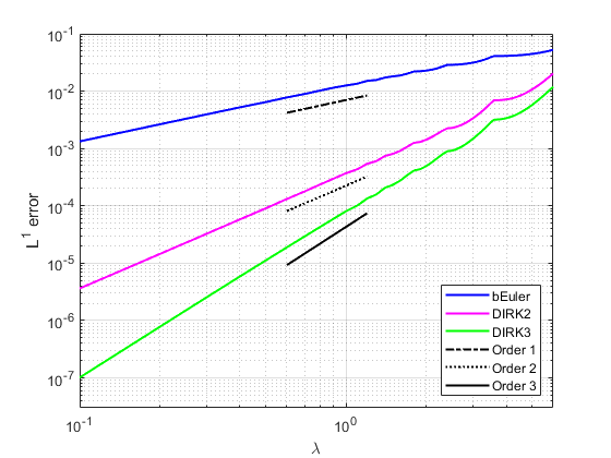
Figure 1: Error plot for (3.1) with initial condition (3.2) using the first-, second- and third-order RAIL schemes. Mesh size $N=200$, tolerance $\epsilon=1.0E-08$, final time $T_{f}=0.5$, initial rank $r^{0}=20$.

The rank of the solution and the relative number number density/mass are shown in Figure 2. For the results in those figures, we use a mesh $N=400$, tolerance $\epsilon=1.0E-08$, time-stepping size $\Delta t=0.3\Delta x$, and initial rank $r^{0}=40$. We also include a reference solution computed with a mesh $N=600$, tolerance $\epsilon=1.0E-08$, time-stepping size $\Delta t=0.1\Delta x$, initial rank $r^{0}=60$, and using DIRK3. We expect the rank-two initial condition (3.2) to instantaneously increase in rank due to the diffusive dynamics. As seen in Figure 2, the RAIL scheme captures this rank increase, with the higher-order schemes better capturing the rank decay towards equilibrium. As one would expect, smaller time-stepping sizes and higher-order time discretizations do a better job at capturing the rank, as seen based on the reference solution. Furthermore, the mass/number density is well-conserved, with the slight changes in mass coming from computing the QR factorization and SVD in equation (2.48) to orthogonalize and diagonalize the final solution after truncation.

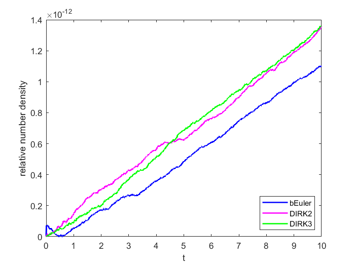
Figure 2: The rank of the solution (left) and relative number density (right) to (3.1) with initial condition (3.2). Mesh size $N=400$, tolerance $\epsilon=1.0E-08$, time-stepping size $\Delta t=0.3\Delta x$, initial rank $r^{0}=40$.

3.2 Rigid body rotation with diffusion

$$u_{t}-yu_{x}+xu_{y}=d(u_{xx}+u_{yy})+\phi,\qquad x,y\in(-2\pi,2\pi)$$ (3.3)

where $\phi(x,y,t)=(6d-4xy-4d(x^{2}+9y^{2}))\text{exp}(-(x^{2}+3y^{2}+2dt))$, the exact solution is $u(x,y,t)=\text{exp}(-(x^{2}+3y^{2}+2dt))$, and $d=1/5$. As seen in Figure 3, we observe the expected accuracies when using the first-, second- and third-order RAIL schemes with IMEX(1,1,1), IMEX(2,2,2) and IMEX(4,4,3), respectively. Notice that the high-order accuracy was still achieved despite the diffusion being smaller in magnitude than the advection. We used a mesh $N=200$, tolerance $\epsilon=1.0E-08$, final time $T_{f}=0.5$, $\lambda$ varying from 0.1 to 2, and initial rank $r^{0}=20$.

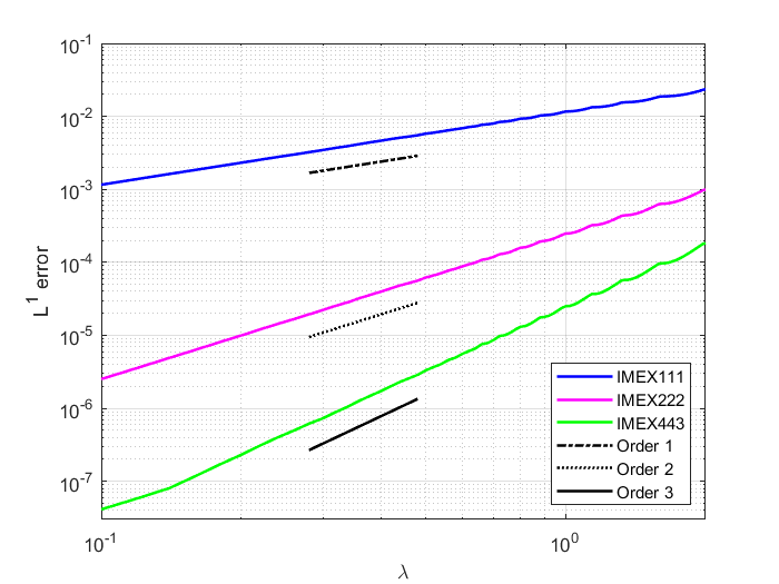
Figure 3: Error plot for (3.3) with initial condition $\text{exp}(-(x^{2}+3y^{2}+2dt))$ using the first-, second- and third-order RAIL schemes. Mesh size $N=200$, tolerance $\epsilon=1.0E-08$, final time $T_{f}=0.5$, initial rank $r^{0}=20$.

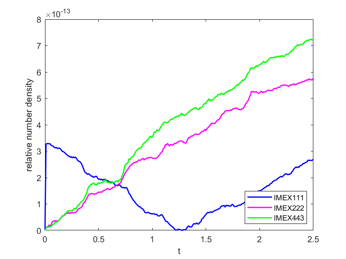
Figure 4: The rank of the solution (left) and relative number density (right) to (3.3) with initial condition $\text{exp}(-(x^{2}+9y^{2}))$. Mesh size $N=200$, tolerance $\epsilon=1.0E-08$, time-stepping size $\Delta t=0.15\Delta x$, initial rank $r^{0}=20$.

Setting $\phi(x,y,t)=0$ and $u(x,y,t=0)=\text{exp}(-(x^{2}+9y^{2}))$, we expect the solution to rotate counterclockwise about the origin while slowly diffusing. Theoretically, the exact rank should be one at $t=0$ and $t=\pi/2$; the rank should be higher in-between these time stamps. The rank of the solution and the relative number number density/mass are shown in Figure 4. For the results in those figures, we use a mesh $N=200$, tolerance $\epsilon=1.0E-08$, time-stepping size $\Delta t=0.15\Delta x$, and initial rank $r^{0}=20$. We also include a reference solution computed with a mesh $N=400$, tolerance $\epsilon=1.0E-08$, time-stepping size $\Delta t=0.05\Delta x$, initial rank $r^{0}=40$, and using IMEX(4,4,3). As seen in Figure 4, the RAIL scheme captures this rank behavior for the first-, second- and third-order schemes. Figure 5 plots the solution at times $t=0$, $t=\pi/4$ and $t=\pi/2$ to better interpret this rank behavior. Lastly, the mass/number density is well-conserved, with the slight changes in mass coming from computing the QR factorization and SVD in equation (2.48) to orthogonalize and diagonalize the final solution after truncation.

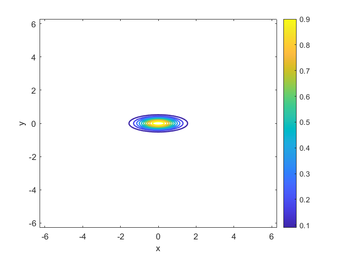
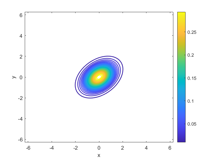
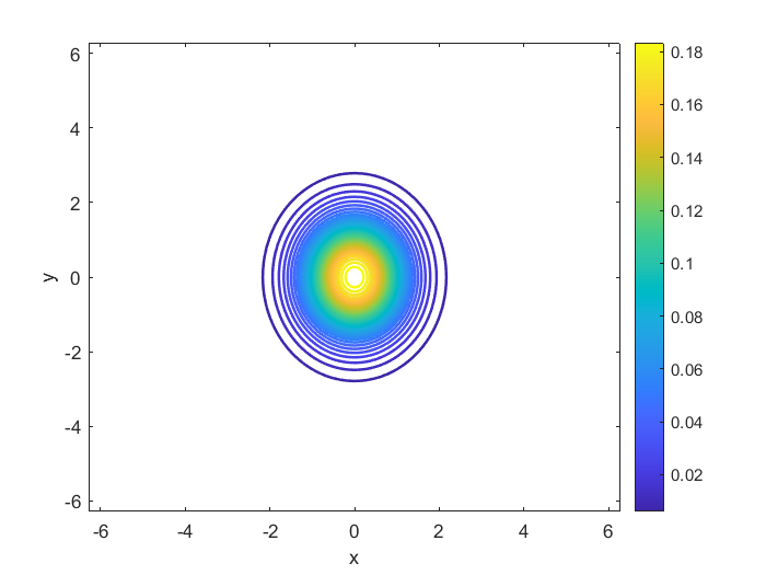
Figure 5: Various snapshots of the numerical solution to equation (3.3) with initial condition $\text{exp}(-(x^{2}+9y^{2}))$. Mesh size $N=200$, tolerance $\epsilon=1.0E-08$, time-stepping size $\Delta t=0.15\Delta x$, initial rank $r^{0}=20$, using IMEX(4,4,3). Times: 0, $\pi/4$, $\pi/2$.

3.3 Swirling deformation with diffusion

$$u_{t}-\big{(}\cos^{2}{(x/2)}\sin{(y)}f(t)u\big{)}_{x}+\big{(}\sin{(x)}\cos^{2}{(y/2)}f(t)u\big{)}_{y}=u_{xx}+u_{yy},\qquad x,y\in(-\pi,\pi)$$ (3.4)

where we set $f(t)=\cos{(\pi t/T_{f})}\pi$. The initial condition is the smooth (with $C^{5}$ smoothness) cosine bell

$$u(x,y,t=0)=\begin{cases}r_{0}^{b}\cos^{6}{\left(\frac{r^{b}(x,y)\pi}{2r_{0}^{b}}\right)},&\text{if}\ r^{b}(x,y)<r_{0}^{b},\\ 0,&\text{otherwise},\end{cases}$$ (3.5)

where $r_{0}^{b}=0.3\pi$ and $r^{b}(x,y)=\sqrt{(x-x_{0}^{b})^{2}+(y-y_{0}^{b})^{2}}$ with $(x_{0}^{b},y_{0}^{b})=(0.3\pi,0)$. Since there is no analytic solution, we use a full-rank reference solution computed with mesh $N=300$, time-stepping size $\Delta t=0.05\Delta x$, and IMEX(4,4,3). As seen in Figure 6, we observe the expected accuracies when using the first-, second- and third-order RAIL schemes with IMEX(1,1,1), IMEX(2,2,2) and IMEX(4,4,3), respectively. We used a mesh $N=100$, tolerance $\epsilon=1.0E-08$, final time $T_{f}=0.5$, $\lambda$ varying from 0.1 to 2, and initial rank $r^{0}=15$.

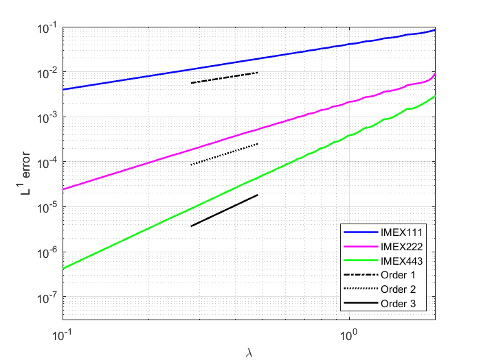
Figure 6: Error plot for (3.4) with initial condition (3.5) using the first-, second- and third-order RAIL schemes. Mesh size $N=100$, tolerance $\epsilon=1.0E-08$, final time $T_{f}=0.5$, initial rank $r^{0}=15$.

Looking at the flow field, we expect the rank to be roughly the same at times $t=0$, $t=T_{f}/2$ and $t=T_{f}$, and to be higher in-between these time stamps. The rank of the solution and the relative number number density/mass are shown in Figure 7. For the results in those figures, we use a mesh $N=300$, tolerance $\epsilon=1.0E-08$, time-stepping size $\Delta t=0.15\Delta x$, and initial rank $r^{0}=30$. We also include a reference solution computed with a mesh $N=300$, tolerance $\epsilon=1.0E-08$, time-stepping size $\Delta t=0.05\Delta x$, initial rank $r^{0}=30$, and using IMEX(4,4,3). As seen in Figure 7, the RAIL scheme was able to capture the first hump and somewhat the second hump. This might be due to the diffusion starting to have a larger influence on the solution around time $t=2.5$. Furthermore, the mass/number density is globally conserved on the order of $1.0E-11$.

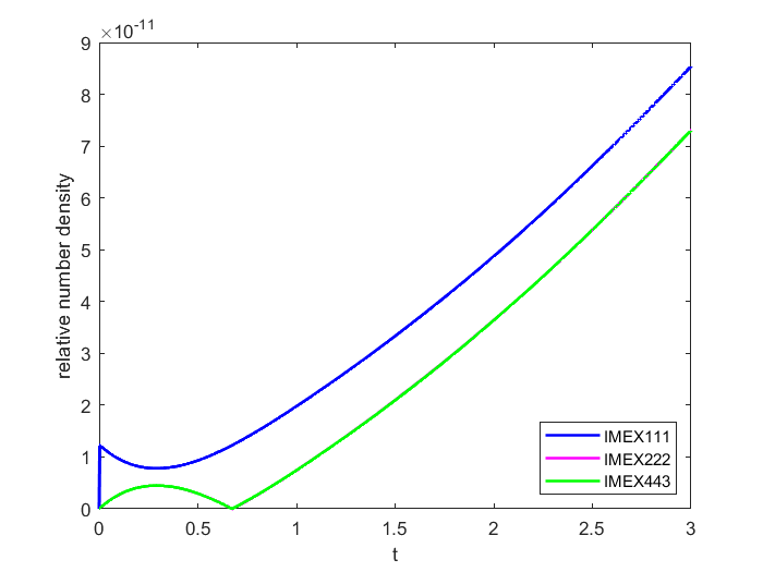
Figure 7: The rank of the solution (left) and relative number density (right) to (3.4) with initial condition (3.5). Mesh size $N=300$, tolerance $\epsilon=1.0E-08$, time-stepping size $\Delta t=0.15\Delta x$, initial rank $r^{0}=30$.

3.4 0D2V Lenard-Bernstein-Fokker-Planck equation

We consider a simplified Fokker-Planck model, the Lenard-Bernstein-Fokker-Planck equation (also known as the Dougherty-Fokker-Planck equation) [34, 35], used to describe weakly coupled collisional plasmas. Restricting ourselves to a single species plasma in 0D2V phase space, that is, zero spatial dimensions and two velocity dimensions, we solve

$$f_{t}-\big{(}(v_{x}-\overline{v}_{x})f\big{)}_{v_{x}}-\big{(}(v_{y}-\overline{v}_{y})f\big{)}_{v_{y}}=D(f_{v_{x}v_{x}}+f_{v_{y}v_{y}}),\qquad v_{x},v_{y}\in(-8,8)$$ (3.6)

with gas constant $R=1/6$, ion temperature $T=3$, thermal velocity $v_{th}=\sqrt{2RT}=\sqrt{2D}=1$, number density $n=\pi$, and bulk velocities $\overline{v}_{x}=\overline{v}_{y}=0$. These quantities were chosen for scaling convenience. The equilibrium solution is the Maxwellian distribution function

$$f_{M}(v_{x},v_{y})=\frac{n}{2\pi RT}\text{exp}\left(-\frac{(v_{x}-\overline{v}_{x})^{2}+(v_{y}-\overline{v}_{y})^{2}}{2RT}\right).$$ (3.7)

Relaxation of the system is tested using the initial distribution function $f(v_{x},v_{y},t=0)=f_{M1}(v_{x},v_{y})+f_{M2}(v_{x},v_{y})$, that is, the sum of two randomly generated Maxwellians such that the total macro-parameters are preserved. The number densities, bulk velocities, and temperatures of the Maxwellians are listed in Table 4. We set $\overline{v}_{y}=0$ so that the two generated Maxwellians are only shifted along the $v_{x}$ axis.

	$f_{M1}$	$f_{M2}$
$n$	1.990964530353041	1.150628123236752
$\overline{v}_{x}$	0.4979792385268875	-0.8616676237412346
$\overline{v}_{y}$	0	0
$T$	2.46518981703837	0.4107062104302872

Table 4: $n=\pi$, $\overline{\mathbf{v}}=\mathbf{0}$, and $T=3$.

We use a mesh $N=300$, time-stepping size $\Delta t=0.15\Delta x$, singular value tolerance $\epsilon=1.0E-06$, and initial rank $r^{0}=30$. We also include a reference solution computed with a mesh $N=400$, tolerance $\epsilon=1.0E-06$, time-stepping size $\Delta t=0.05\Delta x$, initial rank $r^{0}=40$, and using IMEX(4,4,3). Unlike the previous examples, the equilibrium solution to equation (3.6) is a Maxwellian distribution function. To better respect the physics driving the solution to the Maxwellian (3.7) as $t\rightarrow\infty$, we use a Maxwellian distribution for the weight function $w(v_{x},v_{y})$ used to scale the solution in the truncation procedure; see Section 2.3. We use the weight function

$$w(v_{x},v_{y})=w(v_{x})w(v_{y})\coloneqq\big{(}\text{exp}(-v_{x}^{2}/2)+\delta\big{)}\big{(}\text{exp}(-v_{y}^{2}/2)+\delta\big{)},$$ (3.8)

where $\delta=5.0E-09$ is some small robustness parameter to avoid dividing by zero near the boundary. The solution rank and relative number density are shown in Figure 8. Similar to the diffusion equation with initial condition (3.2), we expect the rank-two initial distribution function to immediately increase in rank before decaying towards equilibrium. As seen in Figure 8, the RAIL scheme captures this behavior, and the number density is globally conserved on the order of $1.0E-11$. Furthermore, Figure 9 plots the solution at times $t=0$, $t=0.25$ and $t=1$ to better interpret this rank behavior. Lastly, the RAIL scheme captures the theoretical linear exponential decay of the solution towards relaxation, that is, $\norm{f-f_{M}}_{1}$. As seen in Figure 10, $\norm{f-f_{M}}_{1}$ decays linearly down to $\mathcal{O}(1.0E-10)$, despite the tolerance being $\epsilon=1.0E-06$. This indicates that for this problem, the RAIL scheme preserves the equilibrium solution very well.

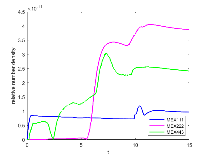
Figure 8: The rank of the solution (left) and relative number density (right) to (3.6) with initial condition $f_{M1}(v_{x},v_{y})+f_{M2}(v_{x},v_{y})$. Mesh size $N=300$, tolerance $\epsilon=1.0E-06$, time-stepping size $\Delta t=0.15\Delta x$, initial rank $r^{0}=30$.

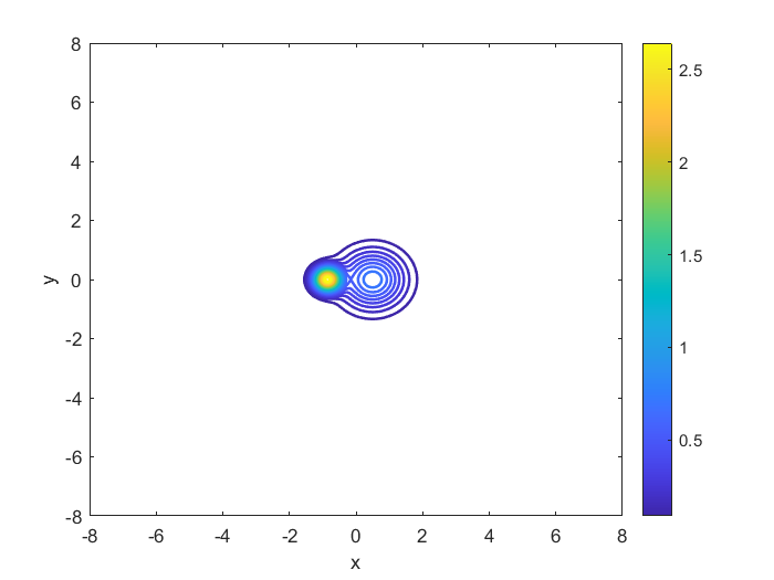
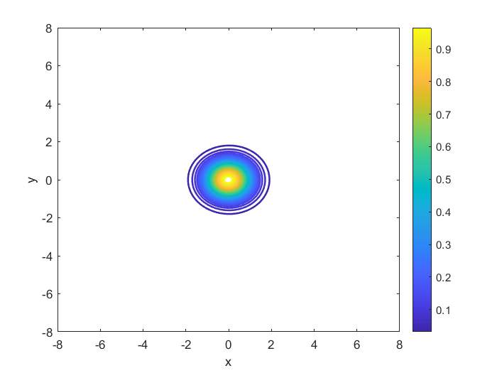
Figure 9: Various snapshots of the numerical solution to equation (3.6) with initial condition $f_{M1}(v_{x},v_{y})+f_{M2}(v_{x},v_{y})$. Mesh size $N=300$, tolerance $\epsilon=1.0E-06$, time-stepping size $\Delta t=0.15\Delta x$, initial rank $r^{0}=30$, using IMEX(4,4,3). Times: 0, 0.25, 1.

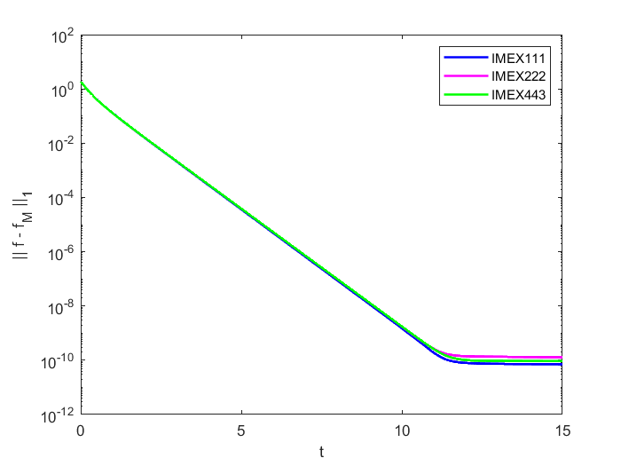
Figure 10: Error plot for (3.6) with initial condition $f_{M1}(v_{x},v_{y})+f_{M2}(v_{x},v_{y})$. Mesh size $N=300$, tolerance $\epsilon=1.0E-06$, final time $T_{f}=15$, $\lambda=0.15$.

4 Conclusion

In this paper, we proposed a reduced augmentation implicit low-rank (RAIL) integrator for solving advection-diffusion equations and Fokker-Planck models. Both implicit and implicit-explicit Runge-Kutta methods were implemented. The partial differential equations were fully discretized into matrix equations in the method-of-lines approach. By spanning the low-order prediction (or updated) bases with the bases from the previous Runge-Kutta stages in a reduced augmentation procedure, the matrix equation was projected onto a richer space. A globally mass conservative truncation procedure was then applied to truncate the solution and keep as low rank as possible. Several tests demonstrated the RAIL scheme’s ability to achieve high-order accuracy, capture solution rank, and conserve mass. Ongoing and future work includes extending the algorithm to higher dimensions through other low-rank tensor decompositions.

Appendix

Butcher tables for DIRK and IMEX methods [39, 37]

Table 5: *

DIRK2 $\nu$ $\nu$ 0 1 $1-\nu$ $\nu$ $1-\nu$ $\nu$

Let $\nu=1-\sqrt{2}/2$.

Table 6: *

DIRK3 $\nu$ $\nu$ 0 0 $\frac{1+\nu}{2}$ $\frac{1-\nu}{2}$ $\nu$ 0 1 $\beta_{1}$ $\beta_{2}$ $\nu$ $\beta_{1}$ $\beta_{2}$ $\nu$

Let $\nu\approx 0.435866521508459$,

$\beta_{1}=-\frac{3}{2}\nu^{2}+4\nu-\frac{1}{4}$,

and $\beta_{2}=\frac{3}{2}\nu^{2}-5\nu+\frac{5}{4}$.

Table 7: *

IMEX(1,1,1) – Implicit Table 0 0 0 1 0 1 0 1

Table 8: *

IMEX(1,1,1) – Explicit Table 0 0 0 1 1 0 1 0

Table 9: *

IMEX(2,2,2) – Implicit Table 0 0 0 0 $\nu$ 0 $\nu$ 0 1 0 $1-\nu$ $\nu$ 0 $1-\nu$ $\nu$

Table 10: *

IMEX(2,2,2) – Explicit Table 0 0 0 0 $\nu$ $\nu$ 0 0 1 $\delta$ $1-\delta$ 0 $\delta$ $1-\delta$ 0

Table 11: *

Let $\nu=1-\sqrt{2}/2$ and $\delta=1-1/(2\nu)$.

Table 12: *

IMEX(4,4,3) – Implicit Table 0 0 0 0 0 0 1/2 0 1/2 0 0 0 2/3 0 1/6 1/2 0 0 1/2 0 -1/2 1/2 1/2 0 1 0 3/2 -3/2 1/2 1/2 0 3/2 -3/2 1/2 1/2

Table 13: *

IMEX(4,4,3) – Explicit Table 0 0 0 0 0 0 1/2 1/2 0 0 0 0 2/3 11/18 1/18 0 0 0 1/2 5/6 -5/6 1/2 0 0 1 1/4 7/4 3/4 -7/4 0 1/4 7/4 3/4 -7/4 0

References

- [1] H.-D. Meyer, U. Manthe and L.. Cederbaum “The multi-configurational time-dependent Hartree approach” In Chem. Phys. Letters 165 Elsevier, 1990, pp. 73–78
- [2] C. Lubich “From quantum to classical molecular dynamics: reduced models and numerical analysis” Zürich: European Mathematical Society, 2008
- [3] O. Koch and C. Lubich “Dynamical Low-Rank Approximation” In SIAM J. Matrix Anal. Appl. 29, 2007, pp. 434–454 DOI: 10.1137/050639703
- [4] E. Kieri, C. Lubich and H. Walach “Discretized dynamical low-rank approximation in the presence of small singular values” In SIAM J. Numer. Anal. 54.2, 2016, pp. 1020–1038
- [5] A. Nonnenmacher and C. Lubich “Dynamical low-rank approximation: applications and numerical experiments” In Math. Comput. Simul. 79.4 Elsevier, 2008, pp. 1346–1357
- [6] C. Lubich and I.V. Oseledets “A projector-splitting integrator for dynamical low-rank approximation” In BIT Numer. Math. 54, 2014, pp. 171–188 DOI: 10.1007/s10543-013-0454-0
- [7] G. Ceruti and C. Lubich “An unconventional robust integrator for dynamical low-rank approximation” In BIT Numer. Math. 62, 2022, pp. 23–44
- [8] L. Einkemmer and C. Lubich “A Low-Rank Projector-Splitting Integrator for the Vlasov–Poisson Equation” In SIAM J. Sci. Comput. 40, 2018, pp. B1330–B1360
- [9] F. Cassini and L. Einkemmer “Efficient 6D Vlasov simulation using the dynamical low-rank framework Ensign” In einkemmer huComput. Phys. Commun. 280 Elsevier, 2022, pp. 108489
- [10] Wei Guo and Jing-Mei Qiu “A low rank tensor representation of linear transport and nonlinear Vlasov solutions and their associated flow maps” In Journal of Computational Physics 458, 2022, pp. 111089 DOI: 111089
- [11] Abram Rodgers, Alec Dektor and Daniele Venturi “Adaptive integration of nonlinear evolution equations on tensor manifolds” In Journal of Scientific Computing 92.2 Springer, 2022, pp. 39
- [12] Wei Guo and Jing-Mei Qiu “A conservative low rank tensor method for the Vlasov dynamics” In SIAM Journal on Scientific Computing, accepted
- [13] Abram Rodgers and Daniele Venturi “Implicit integration of nonlinear evolution equations on tensor manifolds” In J. Sci. Comput., 2023
- [14] C. Lubich “Time integration in the multiconfiguration time-dependent Hartree method of molecular quantum dynamics” In Appl. Math. Res. Express. AMRX 2015 Oxford University Press, 2015, pp. 311–328
- [15] H.-D. Meyer, F. Gatti and G.. Worth “Multidimensional quantum dynamics” John Wiley & Sons, 2009
- [16] K. Kormann “A semi-Lagrangian Vlasov solver in tensor train format” In SIAM J. Sci. Comput. 37, 2015, pp. 613–632 DOI: 10.1137/140971270
- [17] L. Einkemmer, A. Ostermann and C. Piazzola “A low-rank projector-splitting integrator for the Vlasov–Maxwell equations with divergence correction” In J. Comput. Phys. 403 Elsevier, 2020, pp. 109063
- [18] F. Allmann-Rahn, R. Grauer and K. Kormann “A parallel low-rank solver for the six-dimensional Vlasov–Maxwell equations” In J. Comput. Phys. 469 Elsevier BV, 2022, pp. 111562 DOI: 10.1016/j.jcp.2022.111562
- [19] L. Einkemmer “Accelerating the simulation of kinetic shear Alfvén waves with a dynamical low-rank approximation” In arXiv:2306.17526 arXiv, 2023 DOI: 10.48550/ARXIV.2306.17526
- [20] Zhuogang Peng, Ryan G. McClarren and Martin Frank “A low-rank method for two-dimensional time-dependent radiation transport calculations” In Journal of Computational Physics 421, 2020, pp. 109735
- [21] L. Einkemmer, J. Hu and L. Ying “An Efficient Dynamical Low-Rank Algorithm for the Boltzmann-BGK Equation Close to the Compressible Viscous Flow Regime” In SIAM J. Sci. Comput. 43.5 Society for Industrial & Applied Mathematics (SIAM), 2021, pp. B1057–B1080 DOI: 10.1137/21m1392772
- [22] J. Coughlin and J. Hu “Efficient dynamical low-rank approximation for the Vlasov-Ampère-Fokker-Planck system” In J. Comput. Phys. 470 Elsevier BV, 2022, pp. 111590 DOI: 10.1016/j.jcp.2022.111590
- [23] J. Kusch, B. Whewell, R. McClarren and M. Frank “A low-rank power iteration scheme for neutron transport critically problems”, 2022
- [24] T. Jahnke and W. Huisinga “A Dynamical Low-Rank Approach to the Chemical Master Equation” In Bull. Math. Biol. 70.8 Springer ScienceBusiness Media LLC, 2008, pp. 2283–2302 DOI: 10.1007/s11538-008-9346-x
- [25] J. Kusch and P. Stammer “A robust collision source method for rank adaptive dynamical low-rank approximation in radiation therapy” In ESAIM: Mathematical Modelling and Numerical Analysis 57.2 EDP Sciences, 2023, pp. 865–891
- [26] M. Prugger, L. Einkemmer and C.F. Lopez “A dynamical low-rank approach to solve the chemical master equation for biological reaction networks” In J. Comput. Phys. Elsevier BV, 2023, pp. 112250 DOI: 10.1016/j.jcp.2023.112250
- [27] Lukas Einkemmer, Julian Mangott and Martina Prugger “A low-rank complexity reduction algorithm for the high-dimensional kinetic chemical master equation” arXiv, 2023 DOI: 10.48550/ARXIV.2309.08252
- [28] Jan S Hesthaven, Sigal Gottlieb and David Gottlieb “Spectral methods for time-dependent problems” Cambridge University Press, 2007
- [29] Lloyd N Trefethen “Spectral methods in MATLAB” SIAM, 2000
- [30] G. Ceruti, J. Kusch and C. Lubich “A rank-adaptive robust integrator for dynamical low-rank approximation” In BIT Numer. Math. 62 Springer, 2022, pp. 1149–1174
- [31] L. Einkemmer and I. Joseph “A mass, momentum, and energy conservative dynamical low-rank scheme for the Vlasov equation” In J. Comput. Phys. 443 Elsevier, 2021, pp. 110495
- [32] L. Einkemmer, A. Ostermann and C. Scalone “A robust and conservative dynamical low-rank algorithm” In J. Comput. Phys. 484 Elsevier, 2023, pp. 112060
- [33] Wei Guo, Jannatul Ferdous Ema and Jing-Mei Qiu “A Local Macroscopic Conservative (LoMaC) Low Rank Tensor Method with the Discontinuous Galerkin Method for the Vlasov Dynamics” In Communications on Applied Mathematics and Computation, 2023 DOI: 10.1007/s42967-023-00277-7
- [34] JP Dougherty “Model Fokker-Planck equation for a plasma and its solution” In The Physics of Fluids 7.11 American Institute of Physics, 1964, pp. 1788–1799
- [35] Andrew Lenard and Ira B Bernstein “Plasma oscillations with diffusion in velocity space” In Physical Review 112.5 APS, 1958, pp. 1456
- [36] Marshall N Rosenbluth, William M MacDonald and David L Judd “Fokker-Planck equation for an inverse-square force” In Physical Review 107.1 APS, 1957, pp. 1
- [37] E. Hairer and G. Wanner “Solving Ordinary Differential Equations II, Stiff and Differential-Algebraic Problems” Springer Berlin Heidelberg, 1996
- [38] Joseph Nakao “Speeding Up High-Order Algorithms in Computational Fluid and Kinetic Dynamics: Based on Characteristics Tracing and Low-Rank Structures”, 2023
- [39] U.. Ascher, S.. Ruuth and R.. Spiteri “Implicit-explicit Runge-Kutta methods for time-dependent partial differential equations” In Applied Numerical Mathematics 25.2-3, 1997, pp. 151–167
- [40] Richard H. Bartels and George W Stewart “Solution of the matrix equation AX+ XB= C [F4]” In Communications of the ACM 15.9 Association for Computing Machinery (ACM), 1972, pp. 820–826
- [41] Gene Golub, Stephen Nash and Charles Van Loan “A Hessenberg-Schur method for the problem AX+ XB= C” In IEEE Transactions on Automatic Control 24.6 IEEE, 1979, pp. 909–913
- [42] Haijin Wang, Chi-Wang Shu and Qiang Zhang “Stability and error estimates of local discontinuous Galerkin methods with implicit-explicit time-marching for advection-diffusion problems” In SIAM Journal on Numerical Analysis 53.1 SIAM, 2015, pp. 206–227
- [43] Wei Guo and Jing-Mei Qiu “A Local Macroscopic Conservative (LoMaC) low rank tensor method for the Vlasov dynamics” In arXiv preprint arXiv:2207.00518, 2022