OFDMA-F²L: Federated Learning With Flexible Aggregation Over an OFDMA Air Interface

Abstract

Federated learning (FL) can suffer from a communication bottleneck when deployed in mobile networks, limiting participating clients and deterring FL convergence. The impact of practical air interfaces with discrete modulations on FL has not previously been studied in depth. This paper proposes a new paradigm of flexible aggregation-based FL (F²L) over orthogonal frequency division multiple-access (OFDMA) air interface, termed as “OFDMA-F²L”, allowing selected clients to train local models for various numbers of iterations before uploading the models in each aggregation round. We optimize the selections of clients, subchannels and modulations, adapting to channel conditions and computing powers. Specifically, we derive an upper bound on the optimality gap of OFDMA-F²L capturing the impact of the selections, and show that the upper bound is minimized by maximizing the weighted sum rate of the clients per aggregation round. A Lagrange-dual based method is developed to solve this challenging mixed integer program of weighted sum rate maximization, revealing that a “winner-takes-all” policy provides the almost surely optimal client, subchannel, and modulation selections. Experiments on multilayer perceptrons and convolutional neural networks show that OFDMA-F²L with optimal selections can significantly improve the training convergence and accuracy, e.g., by about 18% and 5%, compared to potential alternatives.

I Introduction

As a new framework for distributed online computing and model training, federated learning (FL) has shown significant potential for applications, e.g., Internet-of-Things, autonomous driving, remote medical care, etc. [1]. FL enables individual mobile clients to train a global model collectively without releasing their data [2]. In particular, each client trains its local model independently relying on its local dataset and sends the gradient of the local model to a server. The server aggregates the gradients and broadcasts the aggregated global parameter to assist the clients in their local training.

A challenge faced by FL is the communication bottleneck from the clients to the server, especially when dynamic, lossy, and resource-constrained channels are considered in wireless FL (WFL) [3]. The channels of geographically dispersed clients can differ significantly and change over time, leading to different model uploading delays among the clients. Moreover, the clients can have different computation capabilities, resulting in different local training times, and consequently, different time budgets for model uploading in an FL aggregation round. While more participating clients and hence larger overall training datasets are conducive to better training performance [2], this could lead to a shortage of wireless resources (e.g., bandwidth) for uploading local models. It is crucial to jointly design the local model training and uploading (transmission) schedule of the clients to balance communication and computation.

The transmission schedule of the clients depends on the model aggregation mechanism adopted. Typical synchronous FL (Sync-FL) requires all participating clients to upload their local models (or gradients) for a global aggregation after completing their local training [4]. Alternatively, asynchronous FL (Async-FL) allows each client to upload its local models straightaway after completing its local training. In the latter case, there can be non-negligible gaps between the time the local models are uploaded and the time the global model is broadcast. The computing powers of the clients may not be efficiently exploited. Clients with more powerful computation capability have to wait longer for global model update, especially when there are “stragglers” [5]. Flexible aggregation-based FL (F²L) has recently emerged as a promising solution to the issue of “stragglers”, where clients can train different numbers of iterations before sending their local models synchronously for a global aggregation [6].

The transmission schedule of the clients also depends on their instantaneous computing powers [7]. A client with a weak computing capability has to transmit at a high data rate to complete its local model training and uploading within the same period. Consider a widely-adopted, practical orthogonal-frequency division multiple-access (OFDMA) as the air interface for WFL. Effective selections of the clients, channels, and modulations are key to the transmission schedule. However, the selections form an integer program with discrete variables. This renders the joint optimization of the communication and computation of OFDMA-based WFL systems (for example, OFDMA-based F²L, referred to as “OFDMA-F²L” in this paper) a typically intractable mixed-integer programming problem.

I-A Related Work

Some existing work has focused on the training accuracy, efficiency, and robustness of WFL under a persistent policy of client selection and bandwidth allocation (e.g., see [2, 8, 9, 10, 11, 12]). A partial participating scheme of WFL clients was investigated in [4], where only some clients were chosen to send their local models for global aggregations to minimize the power and time usage of the learning task. A partial synchronization parallel approach was proposed in [3] for a relay-assisted WFL, where local models were uploaded simultaneously and aggregated at relay nodes to reduce traffic. The same convergence speed was achieved as the successive synchronization methods. Yet, none of these studies [8, 9, 10, 11, 12, 4, 3] optimized communication performances for WFL.

Considering the communication performance metrics, energy-efficient WFL has been developed to cope with lossy and dynamically varying wireless environments in [13, 14, 15, 16, 17, 18, 19]. A problem of joint training and communication was constructed in [16] to minimize the overall power usage of a WFL system under a training latency requirement. The optimal resource allocation policy was obtained by using bisection search. In [17], a hierarchical FL architecture was proposed for a heterogeneous cellular system, where the clients were jointly served by macro and micro base stations (BSs). Deep reinforcement learning (DRL) was employed to minimize the power usage under a delay constraint by adjusting client-BS association and resource allocation. Non-orthogonal multiple access (NOMA)-aided FL was examined in [18], where a set of clients formed a NOMA cluster to upload their local models to a BS for model aggregation. The total power usage and FL convergence latency were minimized by jointly optimizing the NOMA transmission, BS broadcast, and FL training accuracy. Resource-constrained WFL with partial aggregation was studied in [19], where stochastic geometry tools were employed to approximately calculate the success probability for each device. All these studies [13, 14, 15, 16, 17, 18, 19] were based on the Sync-FL framework.

The Async-FL framework was proposed to handle clients with different communication and computing capabilities [7, 20, 21, 22, 23, 24, 25]. In [26], Async-FL was developed, which adapted to the heterogeneity of clients regarding their delays in model training and transmitting. The fusion weights of the global aggregation were determined to prevent biased convergence by requiring the weight of each client’s local dataset to be in proportion to its sample number. In [27], an adaptive Async-FL mechanism was developed, where only a small number of the total local updates were collected by the FL server, depending on their arriving order per round. To reduce the mission completion time, DRL was applied to specify the number of aggregated local updates under resource constraints.

An alternative to Async-FL is F²L [6], where clients may have trained for different numbers of iterations when uploading their local models. Different computing powers of the clients can be efficiently leveraged, although persistent global aggregation cycles are maintained as in Sync-FL. However, no consideration has been given to the delays resulting from model uploading under flexible aggregation, which would affect the local training time and performance. Table I summarizes the existing works and highlights the contribution of this work.

In a different yet relevant context, over-the-air (OTA) FL has been investigated to alleviate the communication bottleneck of WFL [28, 29, 30, 31]. For instance, a broadband analog aggregation and transmission scheme was proposed in [28] and [29], where local model gradients were modulated in the analog domain and aggregated by exploiting the waveform-superposition property of radio. An adaptive device scheduling mechanism was developed for OTA-FL in [30], where data quality and energy consumption served as the criteria to select clients for OTA model aggregations to improve the convergence and accuracy of OTA-FL. A new model aggregation method was developed in [31] to align the local model gradients of different devices to resolve the straggler problem in OTA-FL. Moreover, in [32], a decentralized power control policy was designed to enhance the convergence of OTA-FL under fading channels, where stochastic optimization was leveraged to decouple the power control among clients.

TABLE I: Related existing works on WFL and the key contributions of this paper

Related work	Year of publication	Main topic	Difference and improvement of this paper
[4, 3]	2021–2022	Sync-FL with partial synchronization or aggregation	F2L over an OFDMA air interface
[6]	2021	F2L	WFL over an OFDMA air interface
[8, 9, 10, 11, 12]	2020–2023	Sync-FL with persistent client and bandwidth assignments	Selections of client, channel and modulation for OFDMA-F2L
[13, 14, 15, 16, 17]	2020–2023	Joint optimization of communication and computation for Sync-FL	Selections of client, channel and modulation for OFDMA-F2L
[18]	2022	NOMA-aided Sync-FL	F2L over an OFDMA air interface
[19]	2021	Wireless resource-constrained Sync-FL with partial aggregation	Selections of client, channel and modulation for OFDMA-F2L
[7, 20, 21, 22, 23, 24, 25, 26]	2020–2023	Async-FL	F2L over an OFDMA air interface
[27]	2023	Adaptive Async-FL with partial global aggregation	F2L over an OFDMA air interface

I-B Contribution and Organization

This paper proposes the novel OFDMA-F²L approach, where clients can train their local models using different numbers of local iterations before uploading their local models or model gradients to an FL server for a global aggregation via an OFDMA air interface. A new algorithm is proposed to facilitate the convergence of OFDMA-F²L (i.e., to minimize the convergence upper bound), by jointly optimizing the selections of clients, subchannels, and discrete modulations for local training and model uploading, adapting to the channel conditions and computing powers of the clients. The optimal number of local training iterations is accordingly specified per selected client per aggregation round.

The key contributions of this paper can be summarized as follows:

• The OFDMA-F²L approach is proposed, where selected clients train local models, adapting to their available computing powers and times. The clients can also upload their local models concurrently in different subchannels, increasing participating clients and extending their training times.

• We analyze a convergence upper bound on OFDMA-F²L that quantifies the impact of the selections of clients, subchannels, and modulations on the convergence.

• A new problem is formulated to minimize the convergence upper bound of OFDMA-F²L, and transformed to maximize the weighted sum rate of the clients by optimizing the selections of clients, subchannels, and modulations.

• By designing a Lagrange-dual based method, we discover that a “winner-takes-all” policy ensures an optimal selections of clients, subchannels, and modulations almost surely in order to achieve the fast convergence of OFDMA-F²L.

We experimentally evaluate the proposed OFDMA-F²L with the optimal client, subchannel, and modulation selections on multilayer perceptron (MLP) and convolutional neural network (CNN) models and the MNIST, CIFAR10, and Fashion MNIST (FMNIST) datasets. It is shown that OFDMA-F²L with the optimal selections significantly outperforms its alternatives with partially optimal selections or under Sync-FL, e.g., by about 18% and 5%, in convergence and training accuracy on the MLP model.

The remainder of this paper is organized as follows. Section II sets forth the system model. Section III formulates the problem of interest. Section IV analyzes the convergence bound of the proposed algorithm. Section V obtains the optimal assignments of clients, subchannels, and modulations. The OFDMA-F²L system is numerically evaluated in Section VI, followed by conclusions in Section VII. The notations used in this paper is collected in Table II.

TABLE II: List of notations

Notation	Definition
$\bm{\omega}$, ${\bm{\omega}}^{*}$	Global model parameter and optimal global model parameter of OFDMA-F2L, respectively
${\cal D}_{m}$, ${\cal D}$	Local dataset at client $m$, and the collection of all local datasets, respectively
$F(\bm{\omega})$	Global loss function of OFDMA-F2L
$\nabla F(\cdot)$	Gradient of a function $F(\cdot)$
$t,~{}T$	Index and total iteration numbers of OFDMA-F2L
$A$	Maximum number of local iterations between two consecutive aggregations
$\tau,~{}G$	Index and maximum number of aggregations
$M,~{}\cal M$	Number and set of clients
$K,~{}{\cal K}$	Number and set of subchannels
$L,~{}{\cal L}$	Number and set of modulations
$h_{m,k}$	The coefficient of subchannel from client $m$ to the BS
${n}_{m,k}$	CSCG noise with zero mean and variance $\sigma^{2}$
$\lambda_{m,k,l}$	Binary selection indicator indicating the selection of client $m$ and modulation $l$ in subchannel $k$
$\zeta_{m}$, $\bm{\zeta}$	Selection indicator of Client $m$ and the set of selection indicators for all clients, respectively
$r_{l}$	Data rate of modulation $l$
$p_{m,k,l}$	Transmit power of client $m$ in subchannel $k$ when modulation $l$ is used
$P_{m}^{\max}$	Power budget of client $m$
$\chi_{m,k,l}$	BER of the signals uploaded by client $m$ using subchannel $k$ and modulation $l$
$\chi_{0}$	Required BER

II System Model and Assumptions

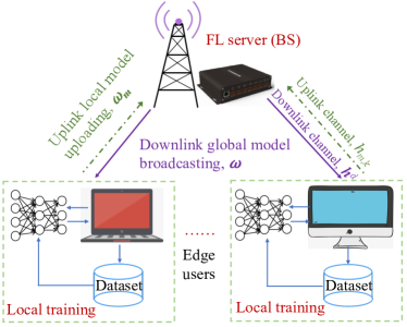
Figure 1: The proposed OFDMA-F²L, where a BS serves as the FL server and multiple clients act as clients. The selected clients send their local models to the BS using OFDMA.

We consider flexible aggregation-based FL in an OFDMA system, i.e., OFDMA-F²L, as shown in Fig. 1, where a BS serving as a central server connects $M$ edge clients over $K$ orthogonal subchannels. The BS and clients all have a single antenna. We use ${\cal M}=\{1,\cdots,M\}$ and ${\cal K}=\{1,\cdots,K\}$ to represent the sets of clients and subchannels, respectively. The BS wishes to learn a machine learning (ML) model using the datasets stored at the clients, since the clients are reluctant to share their data for privacy concerns. As a result, the clients train and transmit their local models to the BS via the uplink OFDMA subchannels, one client per subchannel.

Upon the receipt of the local models, the BS aggregates them into a global model and distributes the global model to the clients through a downlink broadcast. Considering limited communication and computation resources, only some clients are chosen to train and upload their local models. The BS performs client selection and resource allocation.

II-A F²L Model

Let ${\cal D}_{m}$ denote the local dataset at client $m\in{\cal M}$, and $D_{m}=|{\cal D}_{m}|$ denote the size of the local dataset, where $|\cdot|$ stands for cardinality. ${\cal D}=\underset{\forall m\in{\cal M}}{\cup}{\cal D}_{m}$ collects all local datasets at the clients with $D=|{\cal D}|=\sum_{m\in{\cal M}}D_{m}$ being the size of ${\cal D}$. Assume that each client $m$ divides its local dataset ${\cal D}_{m}$ into multiple independent and identically distributed (i.i.d.) mini-batches with the same distribution as ${\cal D}_{m}$. $F_{m}(\bm{\omega};{\cal X})$ is the loss function of client $m\in{\cal M}$, measuring the model error on the client’s dataset ${\cal X}\subseteq{\cal D}_{m}$. Here, $\bm{\omega}$ is the global model parameter vector. The global loss function at the BS, denoted by $F(\bm{\omega})$, is acquired by gathering the local models uploaded from the selected clients, as given by

$${\bm{\omega}}^{*}=\arg\underset{\bm{\omega},\,\{\zeta^{\tau},\forall\tau\}}{\min}~{}F({\bm{\omega}}),$$ (1)

with $$F({\bm{\omega}})\triangleq\frac{1}{B}\sum_{m\in{\cal M}}\sum_{{\tau}}\varrho^{\tau}_{m}\zeta^{\tau}_{m}F_{m}({\bm{\omega}};{\cal B}^{\tau}_{m}),$$

where $\bm{\omega}^{*}$ is the optimal model parameter minimizing $F(\bm{\omega})$; ${\bm{{\cal B}}}^{\tau}_{m}\subseteq{\cal D}_{m}$ collects the set of mini-batches sampled from the local dataset ${\cal D}_{m}$ during the $\tau$-th aggregation round; $B=\sum_{m}\sum_{\tau}I^{\tau}_{m}$ and $I^{\tau}_{m}$ is the number of local training iterations at client $m$ in the $\tau$-th aggregation round. $\varrho^{\tau}_{m}=\frac{A}{I^{\tau}_{m}}\cdot\frac{D_{m}}{D}$ is the aggregation coefficient of client $m$ for the $\tau$-th aggregation of F²L, where $A$ is the maximum number of iterations a client can train locally per aggregation round and $I^{\tau}_{m}\leq A$. In this sense, greater aggregation coefficients can be given to clients that train fewer iterations in an aggregation round, compensating for the additional iterations other clients completed and contributing to unbiased gradient after aggregation [6, Sec. 4.1, Scheme C].

Here, $\bm{\zeta^{\tau}}=\{\zeta^{\tau}_{1},\cdots,\zeta^{\tau}_{M}\}$ collects the client selection indicators with $\zeta^{\tau}_{m}$ indicating client $m$ is selected for the $\tau$-th aggregation; i.e., $\zeta^{\tau}_{m}=1$ if client $m$ is selected; otherwise, $\zeta^{\tau}_{m}=0$. The client selection is critical for FL, especially when the communication and computation resources are constrained. Not all clients can upload their local models to the BS.

OFDMA-F²L supports flexible aggregation at the BS [6], where the clients can execute different numbers of local iterations per aggregation round and, if selected, transmit their latest local models to the BS for a synchronous global model aggregation (in other words, the clients complete uploading their local models at the same time so that the global aggregation can start straightaway). The FL process is divided evenly into $G$ global aggregations. Each aggregation round lasts for the same duration. The OFDMA-F²L contains three alternating steps:

• Local Model Training: After the $\tau$-th global model aggregation ($\tau=1,\cdots,G$), each selected client $m$ ($\zeta^{\tau}_{m}=1$) performs $I^{\tau}_{m}$ iterations of local training. The local training of each selected client $m$ for the $(\tau+1)$-th global aggregation is initialized to be $\bm{\omega}^{\tau}_{m}(0)=\bm{\omega}^{\tau}$, with $\bm{\omega}^{\tau}$ being the global model acquired in the $\tau$-th global model aggregation. The local model of client $m$ at the $i$-th iteration ($i=1,\cdots,I^{\tau}_{m}$), denoted by $\bm{\omega}^{\tau}_{m}(i)$, is refreshed by

  $$\bm{\omega}^{\tau}_{m}(i)={\bm{\omega}}^{\tau}_{m}(i-1)-\eta\nabla F_{m}\left({\bm{\omega}}^{\tau}_{m}(i-1);{\cal B}^{\tau}_{m}(i-1)\right),$$ (2)

  where $\eta$ is the learning rate, and ${\bm{{\cal B}}}^{\tau}_{m}=\{{{\cal{B}}}^{\tau}_{m}(0),\cdots,{\cal B}^{\tau-1}_{m}(I^{\tau}_{m}-1)\}$ collects all mini-batches sampled from the local dataset ${\cal D}_{m}$. ${\cal B}^{\tau}_{m}(i)$ is the mini-batch used by device $m$ for the $i$-th local iteration of the $\tau$-th global aggregation.

• Global Aggregation: The clients selected by the BS upload their local models for the $(\tau+1)$-th global model aggregation after their local training. The global model obtained is

  $$\bm{\omega}^{\tau+1} =\sum_{m\in{\cal M}}\varrho^{\tau}_{m}\zeta^{\tau}_{m}{\bm{\omega}^{\tau}_{m}}$$ (3)

  $$=\sum_{m\in{\cal M}}\varrho^{\tau}_{m}\zeta^{\tau}_{m}\left(\sum^{I^{\tau}_{m}-1}_{i=0}\left({\bm{\omega}^{{\tau}}_{m}{(i)}}-\eta\nabla F_{m}({\bm{\omega}}^{\tau}_{m}{(i)};{\cal B}^{\tau}_{m}{(i)})\right)\right).$$

• Global Model Update: The BS broadcasts the global model $\bm{\omega}^{\tau}$ and selects the clients for the next global aggregation. Then, the selected clients start their local training iterations based on $\bm{\omega}^{\tau}$.

Algorithm 1 summarizes the OFDMA-F²L method. As will be described in Section IV-A, we assume a convex loss function of the ML task, and hence, OFDMA-F²L converges. Suppose that the optimal ML model parameter $\bm{\omega}^{*}$ can be acquired after $G$ global aggregations. $F(\bm{\omega}^{*})$ provides the minimum global loss. Nevertheless, when the loss function is non-convex, OFDMA-F²L can still converge, as typically observed in the literature, e.g., [20, 25], and numerically validated in Section VI-B. Note that if $I^{\tau}_{m}=A,\forall m\in{\cal M}$, i.e., all selected clients finish a given number of $A$ local iterations (or updates), Algorithm 1 becomes the FedAvg algorithm [33].

Input: $I^{\tau}_{m}$, $G$, $\bm{\omega}^{0}$, $\epsilon$, $\delta$, and $C$.

Output: $\bm{\omega}^{T}$.

1 Initialize: $t=0$, $\bm{\omega}^{0}$;

2 for $\tau=1:G$ do

3       while $i\leq I^{\tau}_{m}$ do

             // Local model update

4              $\bm{\omega}^{\tau}_{m}(i)={\bm{\omega}}^{\tau}_{m}(i-1)-\eta\nabla F_{m}({\bm{\omega}}^{\tau}_{m}(i-1))$;

5             Clip the local parameters:    $\bm{\omega}^{\tau}_{m}(i)=\bm{\omega}^{\tau}_{m}(i)/\max\left(1,\frac{\left\|\bm{\omega}^{\tau}_{m}(i)\right\|}{C}\right)$;

6             $i\leftarrow i+1$;

      // Global model aggregation

7      

8       Update the global model parameters: $\bm{\omega}^{\tau}=\sum_{m\in{\cal M}}\varrho^{\tau}_{m}\zeta^{\tau}_{m}\bigg{(}\sum^{I^{\tau}_{m}-1}_{i=0}\Big{(}{\bm{\omega}^{{\tau}}_{m}{(i)}}-\eta\nabla F_{m}({\bm{\omega}}^{\tau}_{m}{(i)};{\cal B}^{\tau}_{m}{(i)})\Big{)}\bigg{)}$;

9       Update the local model parameters:   ${\bm{\omega}}^{\tau}_{m}(0)=\bm{\omega}^{\tau},\;\forall m\in{\cal M}$;

10      

Algorithm 1 OFDMA-F²L.

II-B Transmission Model

At the beginning of an aggregation round, the BS selects the clients, subchannels, and modulation modes based on the channel state information (CSI) and computing powers that the clients fed back at the end of the previous aggregation round. Then, the BS broadcasts the selections and the global model aggregated at the end of the previous aggregation round, e.g., using its lowest non-zero modulation mode and full transmit power. As a result, all clients are expected to reliably receive the global model and the selections/schedule. The downlink delay, denoted by $T^{\text{DL}}$, is given. The global and local models have the same size, that is, $|\bm{\omega}|=|\bm{\omega}_{m}|$.

Towards the end of each aggregation round, the selected clients upload their local models using an OFDMA protocol. Let ${\mathbf{x}}_{k}^{\tau}\triangleq\left[x_{1,k}^{\tau},\cdots,x_{M,k}^{\tau}\right]^{T}\in{\mathbb{C}^{M\times 1}}$ represent the signals that each of the $M$ clients would send in subchannel $k$, if it is allocated with the subchannel at the $\tau$-th aggregation round. Consider Rayleigh fading, the channel gain of client $m$ in subchannel $k$ is

$$h_{m,k}^{\tau}=\sqrt{\epsilon_{o}\left(d_{m}\right)^{-\alpha}}\tilde{h}^{\tau},~{}\forall m,k,$$ (4)

where $\tilde{h}^{\tau}$ is a random scattering element captured by zero-mean and unit-variance circularly symmetric complex Gaussian (CSCG) variables. $\epsilon_{o}$ is the path loss at the reference distance $d_{0}=1$ m. $\alpha$ is the path loss exponent. $d_{m}$ is the distance between client $m$ and the BS.

Assume that the channels experience block fading, i.e., the channels stay the same within a global aggregation round and vary independently between aggregation rounds [34]. At the ${\tau}$-th aggregation round, the received SNR at the BS from client $m$ in subchannel $k$ is given by

$$\gamma_{m,k}^{\tau}=\frac{p_{m,k}^{\tau}|h_{m,k}^{\tau}|^{2}}{\sigma^{2}},$$ (5)

where $p_{m,k}^{\tau}$ is the transmit power of client $m$ in subchannel $k$, and $\sigma^{2}$ is the variance of the zero-mean CSCG noise ${n}_{m,k}^{\tau}$, i.e., ${n}_{m,k}^{\tau}\in{\cal CN}\left(0,\sigma^{2}\right)$.

Each client can take a modulation mode from a discrete set of $L$ modulation modes. The set is denoted by ${\cal L}=\{0,1,\cdots,L\}$, where $L=|\mathcal{L}|$ and $|\cdot|$ stands for cardinality. The data rate of modulation $l$ is represented by $r_{l}$. $l=0$ indicates no transmission, i.e., $r_{0}=0$. At the BS, the bit error rate (BER) of the local model from client $m$ using subchannel $k$ and modulation $l$ is [35]

$$\chi_{m,k,l}^{\tau}=\beta_{1}\exp\left(-\frac{\beta_{2}\gamma_{m,k}^{\tau}}{2^{r_{l}}-1}\right),$$ (6)

where $\beta_{1}$ and $\beta_{2}$ are constants relying on the modulation.

To ensure the local model parameters transmitted from client $m$ to the BS using subchannel $k$ and modulation $l$ achieve the required BER $\chi_{0}$, the minimum transmit power required is [36]

$$p_{m,k,l}^{\tau}=\frac{\left(2^{r_{l}}-1\right)\ln\left(\frac{\beta_{1}}{\chi_{0}}\right)\sigma^{2}}{\beta_{2}\left|h_{m,k}^{\tau}\right|^{2}},$$ (7)

which is acquired by outplacing $\chi_{m,k,l}^{\tau}$ with $\chi_{0}$ in (6) and then substituting (5) into (6), followed by rearranging (6). Here, we choose a sufficiently small value of $\chi_{0}$ (e.g., $\leq 10^{-6}$). In other words, the BS receives reasonably accurate and reliable local models.

Let $\lambda_{m,k,l}^{\tau}=1$ denote the assignment of subchannel $k$ and modulation $l$ to client $m$ to upload its local model, given $|h_{m,k}^{\tau}|^{2}$; and $\lambda_{m,k,l}^{\tau}=0$ denotes otherwise. Let $\bm{\lambda}^{\tau}:=\left\{\lambda_{m,k,l}^{\tau},\;\forall m\in{\cal M},\;k\in{\cal K},\;l\in{\cal L}\right\}$ represent the collection of all indicators to be optimized in the $\tau$-th aggregation round. The data rate of client $m$ is obtained as

$$R^{\text{UL},\tau}_{m}=\sum_{k=1}^{K}\sum_{l=0}^{L}\lambda_{m,k,l}^{\tau}\times r_{l}.$$ (8)

According to the minimum transmit power specified in (7), the transmit power of client $m$ is

$$P_{m}^{\tau}=\sum_{k=1}^{K}\sum_{l=0}^{L}\lambda_{m,k,l}^{\tau}\times p_{m,k,l}^{\tau}.$$ (9)

The delay for client $m$ to upload its local model is

$$T^{\text{UL},\tau}_{m}=\frac{|\bm{\omega}_{m}|}{R^{\text{UL},\tau}_{m}}=\frac{|\bm{\omega}_{m}|}{\sum_{k=1}^{K}\sum_{l=0}^{L}\lambda_{m,k,l}^{\tau}\times r_{l}},$$ (10)

where $|\bm{\omega}_{m}|$ is the size of client $m$’s local model (in bits).

II-C Computing Model

We adopt the number of floating-point operations (FLOPs) to reflect the computational capability of the clients. $\mu$ denotes the number of FLOPs required to train a local model relying on a mini-batch of a local dataset. In the $\tau$-th aggregation round, the number of FLOPs required for client $m$ is $\mu_{m}^{\tau}=\mu I_{m}^{\tau}$. The local training delay of client $m$ is

$$T^{{\rm C},\tau}_{m}=\frac{\mu_{m}^{\tau}}{\beta_{m}}=\frac{\mu I_{m}^{\tau}}{\beta_{m}}.$$ (11)

Here, $\beta_{m}$ is the computational (or processing) speed of client $m$.

As per any global aggregation $\tau$, the total delay undergone by client $m$ is given by

$$T_{m}^{\tau}=T^{{\rm C},\tau}_{m}+T^{\text{UL},\tau}_{m}+T^{\text{DL}},$$ (12)

which considers both the transmission and computation delays. Given the equal duration of each FL round, if the uplink and downlink delays are longer, there is a shorter time for local model training. If the computing delay is longer per iteration, the client can only complete fewer iterations. This impacts the convergence and accuracy of the training.

III Problem Statement

We propose to jointly design the selection of clients, subchannels and modulations, i.e., $\bm{\lambda}^{\tau}$, to minimize the global loss function of the OFDMA-F²L system per aggregation round, i.e., the $\tau$-th round. The problem is formulated as

$$\textbf{P1}:\;\min_{\{\bm{\lambda}^{\tau},{\bm{\omega}}\}}\;\; \sum_{m\in{\cal M}}\frac{D_{m}\zeta_{m}^{\tau}F_{m}({\bm{\omega}})}{D}$$ (13a)

s.t. $$\zeta_{m}^{\tau}={\rm sgn}\left(\sum_{k=1}^{K}\sum_{l=0}^{L}\lambda_{m,k,l}^{\tau}\right),$$ (13b)

$$P_{m}^{\tau}\leq P^{\max}_{m},\forall m,$$ (13c)

$$\sum_{k=1}^{K}\sum_{m=1}^{M}\sum_{l=0}^{L}\lambda_{m,k,l}^{\tau}\leq K,$$ (13d)

$$\sum_{m=1}^{M}\sum_{l=0}^{L}\lambda_{m,k,l}^{\tau}\leq 1,~{}\forall k,$$ (13e)

$$\lambda_{m,k,l}^{\tau}\in\{0,1\},$$ (13f)

$$T_{m}^{\tau}\leq T_{\rm th},$$ (13g)

where ${\rm sgn}(\cdot)$ is the sign function. The objective (13a) stems from (1). Specifically, (1) minimizes the global loss function over all aggregation rounds. (13a) decouples the minimization over time and optimizes the variables and parameters for each round, which is in line with practical FL implementations resulting from causality. Hence, constraint (13b) yields

(14b)

In other words, client $m$ is selected if at least one subchannel and modulation are allocated to the client. Constraint (13c) indicates that the sum transmit power of each client is upper bounded by $P^{\max}_{m}$. (13d) specifies that the number of subchannels allocated to all clients is no greater than $K$. Constraint (13e) ensures that a subchannel is allocated to at most one client to avoid inter-client interference. (13g) indicates that the delay (including communication and computation delay) required to conduct the F²L is upper bounded by a pre-specified threshold, i.e., $T_{\rm th}$, for each global aggregation.

The determination of $\lambda_{m,k,l}^{\tau}$ relies on not only the transmission rate (or time), but also the computing capability of each client. This indicates that the computing time $T_{m}^{\rm C,\tau}$ or the number of iterations per selected client $I_{m}^{\tau}$ is also optimized implicitly by solving problem P1 per round $\tau$. Once $\lambda_{m,k,l}^{\tau}$ is decided, the transmit power of client $m$ using subchannel $k$ and modulation $l$, that is, (7), is set to satisfy the BER requirement.

Problem P1 is new, yet mathematically intractable. It is non-convex in $\bm{\lambda}^{\tau}$ and ${\bm{\omega}}$, and has a mixed integer programming nature resulting from the client selection and subchannel assignment. Moreover, the global loss function $F({\bm{\lambda}^{\tau}},{\bm{\omega}})$ is non-convex and has a large number of parameters to be optimized. As a consequence, problem P1 cannot be directly solved using conventional optimization methods, such as alternating optimization and successive convex approximation.

We decouple problem P1 between the global model learning, and the assignments of the client and modulation mode per subchannel. We first derive the convergence upper bound of the global loss function of OFDMA-F²L, i.e., $F({\bm{\omega}})$, and then derive the almost surely optimal assignments of clients, channels, and modulations to minimize the upper bound.

IV Convergence Analysis of OFDMA-F²L

This section starts by deriving the optimality gap of OFDMA-F²L. The optimality gap is minimized per communication by optimally selecting clients, channels, and modulations, to encourage the convergence of the OFDMA-F²L, as will be delineated in Section V.

IV-A Definitions and Assumptions

This section establishes the upper bound for the optimality gap of OFDMA-F²L, i.e., Algorithm 1. We start by presenting the definitions and assumptions used.

Definition 1 (Gradient Divergence).

Let $\gamma_{m}$ denote an upper bound of the gradient difference between the local and global loss functions, i.e., $\left\|\nabla F_{m}({\bm{\omega}})-\nabla F({\bm{\omega}})\right\|\leq\gamma_{m}$, $\forall m,\bm{\omega}$. The global gradient divergence is $\gamma\triangleq\frac{\sum_{m}D_{m}\gamma_{m}}{{D}}$.

Assumption 1.

$\forall m\in{\cal M}$, we make the following assumptions:

1. The loss function of FL is smooth. Specifically, the gradient of $F_{m}(\bm{\omega})$ is $L_{c}$-Lipschitz continuous [37], that is, $\left\|\nabla F_{m}({\bm{\omega}}^{\tau+1})-\nabla F_{m}({\bm{\omega}}^{\tau})\right\|\leq L_{c}\left\|{\bm{\omega}}^{\tau+1}-{\bm{\omega}}^{\tau}\right\|,\,\forall{\bm{\omega}}^{\tau},{\bm{\omega}}^{\tau+1}$, with $L_{c}$ being a constant depending on the loss function, so as the gradient of $F({\bm{\omega}})$ is also $L_{c}$-Lipschitz continuous;

2. The learning rate is $\eta\leq\frac{1}{L_{c}}$;

3. The mean squared norm of the stochastic gradients at each edge client $m$ is uniformly bounded by $\mathbb{E}_{\mathcal{B}^{\tau}_{m}}\left\|\nabla F_{m}({\bm{\omega}}^{\tau}_{m}(i);\mathcal{B}^{\tau}_{m}(i))\right\|^{2}\leq\kappa_{1}+\kappa_{2}\|\nabla F(\bm{\omega}^{\tau})\|^{2},\forall m~{}\text{and}~{}\tau$ with $\kappa_{1},\kappa_{2}\geq 0$;

4. $F_{m}(\bm{\omega})$ meets the Polyak-Lojasiewicz condition [38] with a constant $\rho$, implying that $F(\bm{\omega})-F({\bm{\omega}}^{*})\leq\frac{1}{2\rho}\left\|\nabla F(\bm{\omega})\right\|^{2}$;

5. $F({\bm{\omega}}^{0})-F({\bm{\omega}}^{*})=\Theta$, in which $\Theta$ is a constant; in other words, the initial optimality gap is bounded.

These assumptions have been extensively adopted in the literature, e.g., [3, 27, 25]. Many modern ML models have multiple layers and non-convex loss functions (e.g., CNN). Nonetheless, a considerable number of ML tasks, e.g., logistic regression, have (strongly) convex loss functions, e.g., cross-entropy, ordinary least, etc. These convex loss functions satisfy Assumption 1. Many existing algorithms developed under the (strong) convexity assumptions were experimentally validated for ML models with non-convex loss functions, e.g., [27, 25], and references therein.

IV-B Convergence Analysis

Based on Definition 1 and Assumption 1, each local loss function in (1) is strongly convex and hence, OFDMA-F²L converges. We establish the ensuing theorem to evaluate the upper bound for the optimality gap of OFDMA-F²L, i.e., the gap between ${\bm{\omega}}^{\tau}$ and ${\bm{\omega}}^{*}$.

Theorem 1.

After $\tau$ global aggregations, the convergence upper bound of OFDMA-F²L is

$$F({\bm{\omega}}^{\tau}) -F({\bm{\omega}}^{*})\leq(1-2\rho\phi_{2})^{\tau}\Theta+\phi_{1}\frac{1-\left(1-2\rho\phi_{2}\right)^{\tau}}{2\rho\phi_{2}},$$ (14o)

where $\phi_{1}\triangleq\frac{\eta^{2}L_{c}}{2}\sum_{m\in{\cal M}}\frac{A^{2}\kappa_{1}D_{m}^{2}\zeta^{\tau}_{m}}{D^{2}I^{\tau}_{m}}$ and $\phi_{2}\triangleq\eta-\frac{\eta^{2}L_{c}}{2}\sum_{m\in{\cal M}}\frac{A^{2}\kappa_{2}D_{m}^{2}\zeta^{\tau}_{m}}{D^{2}I^{\tau}_{m}}$.

Proof.

See Appendix A. ∎

To ensure the convergence of OFDMA-F²L, the following proposition is developed based on Theorem 1.

Proposition 1.

To guarantee the convergence of OFDMA-F²L, it must hold that $1-2\rho\phi_{2}<1$. Hence, $\kappa_{2}$ must satisfy

$$\kappa_{2}<\frac{2}{\eta L_{c}A^{2}\sum_{m\in{\cal M}}\frac{D^{2}_{m}\zeta^{\tau}_{m}}{D^{2}I^{\tau}_{m}}}\overset{\eta=\frac{1}{L_{c}}}{=}\frac{2}{A^{2}\sum_{m\in{\cal M}}\frac{D^{2}_{m}\zeta^{\tau}_{m}}{D^{2}I^{\tau}_{m}}}.$$ (14p)

This proposition provides a sufficient condition for the convergence of OFDMA-F²L.

Corollary 1.

In the case of $1-2\rho\phi_{2}<1$, as $\tau\to\infty$, the convergence upper bound of OFDMA-F²L is obtained as

$$F({\bm{\omega}}^{\tau})-F({\bm{\omega}}^{*}) \leq\frac{\phi_{1}}{2\rho\phi_{2}}$$ (14qa)

$$=\frac{\eta^{2}L_{c}}{4\rho}\frac{\sum_{m\in{\cal M}}\frac{A^{2}\kappa_{1}D_{m}^{2}\zeta^{\tau}_{m}}{D^{2}I^{\tau}_{m}}}{\eta-\frac{\eta^{2}L_{c}}{2}\sum_{m\in{\cal M}}\frac{A^{2}\kappa_{2}D_{m}^{2}\zeta^{\tau}_{m}}{D^{2}I^{\tau}_{m}}}$$ (14qb)

$$\leq\frac{1}{2\rho}\sum_{m\in{\cal M}}\frac{D_{m}^{2}\zeta^{\tau}_{m}}{D^{2}I^{\tau}_{m}}\propto\sum_{m\in{\cal M}}\frac{D_{m}^{2}\zeta^{\tau}_{m}}{D^{2}I^{\tau}_{m}}.$$ (14qc)

The upper bound is proportional to $\sum_{m\in{\cal M}}\frac{D_{m}^{2}\zeta^{\tau}_{m}}{D^{2}I^{\tau}_{m}}$.

According to Corollary 1, minimizing the optimality gap of OFDMA-F²L is equivalent to minimizing $\sum_{m\in{\cal M}}\frac{D_{m}^{2}\zeta^{\tau}_{m}}{D^{2}I^{\tau}_{m}}$ by optimally selecting clients, channels, and modulations. Consequently, we can reformulate the problem of interest to facilitate the problem-solving in Section V.

V Optimal Client, Channel, and Modulation Selection for OFDMA-F²L

Since the selections of the clients, subchannels, and modulations are performed independently in every aggregation round, i.e., the $\tau$-th aggregation round, we suppress the superscript “^τ” in the rest of this paper for brevity of notation.

According to Theorem 1, minimizing the global loss function can be transformed into minimizing the optimality gap of OFDMA-F²L, i.e., between $F({\bm{\omega}})$ and $F({\bm{\omega}}^{*})$. Since the optimality gap is proportional to $\sum_{m\in{\cal M}}\frac{D_{m}^{2}\zeta_{m}}{D^{2}I_{m}}$ per aggregation round $\tau$, as stated in Corollary 1, problem P1 can be rewritten in a much simpler form, as given by

$$\textbf{P2}:\;\min_{\{\bm{\lambda}\}}\;\; \sum_{m\in{\cal M}}\frac{D_{m}^{2}\zeta_{m}}{D^{2}I_{m}}$$ (14ra)

s.t. $$1\leq I_{m}\leq A,$$ (14rb)

$$\eqref{eq-P1 b1}-\eqref{eq-P1 h}.$$

Problem P2 is still difficult to tackle, as it is a mixed integer program. Moreover, the feasible solution region of the problem is non-convex since the optimization variable $\bm{\lambda}$ is discrete. In the ensuing sections, we first convert the objective function to an explicit function of $\bm{\lambda}$, and then obtain the almost surely optimal solution to the problem.

It is noted that in Problem P2, the number of training iterations per client per round, $I_{m}$, is also optimized while maximizing the objective since it can be uniquely determined given $T_{m}^{\rm C}$ and $T_{m}^{\rm UL}$ (or $\bm{\lambda}$). This indicates that the selections of clients, channels and modulations are based on their available computing powers. In other words, OFDMA-F²L is flexible in the number of training iterations accomplished by each selected client by taking the potentially different and even time-varying computational capabilities of the clients into account. This flexibility enables the algorithm to achieve better efficiency in both communication and computation.

V-A Problem Transformation

We proceed to show that optimizing the local iteration numbers $I_{m}$ can be achieved by optimizing the uplink transmission delay $T_{m}^{\rm UL}$. From (11) and (12), we have

$$I_{m} =T_{m}^{C}\beta_{m}/\mu,$$ (14sa)

$$T^{C}_{m} =T_{m}-T^{\rm UL}_{m}-T^{\rm DL}.$$ (14sb)

Substituting (14sb) into (14sa), we have

$$I_{m}=(T_{m}-T^{\rm UL}_{m}-T^{\rm DL})\beta_{m}/\mu.$$ (14t)

Here, $I_{m}$ increases with $T_{m}$; $T^{\rm DL}$ and $\mu$ are given.

For the set of selected clients, i.e., $\cal M^{\prime}\in\cal M$ ($|{\cal M^{\prime}}|=M^{\prime}$), we have $\zeta_{m}=1,\,\forall m\in\cal M^{\prime}$. Then, the objective function in (14ra) can be recast as $\sum_{m\in{\cal M^{\prime}}}\frac{D_{m}^{2}}{D^{2}I_{m}}$. Exploiting the harmonic-arithmetic mean inequality (i.e., $\frac{n}{\sum^{n}_{i=1}\frac{1}{x_{i}}}\leq\frac{\sum^{n}_{i=1}{x_{i}}}{n},\,\forall x_{i}>0$), it follows that

$$\sum_{m\in{\cal M^{\prime}}}\frac{D_{m}^{2}}{D^{2}I_{m}} \geq\frac{M^{\prime 2}}{\sum_{m\in{\cal M^{\prime}}}\frac{D^{2}I_{m}}{D_{m}^{2}}}$$ (14ua)

$$=\frac{M^{\prime 2}}{\sum_{m\in{\cal M^{\prime}}}{(T_{m}-T^{\rm UL}_{m}-T^{\rm DL})\beta_{m}D^{2}/\mu D_{m}^{2}}}$$ (14ub)

$$\geq\frac{M^{\prime 2}}{\sum_{m\in{\cal M^{\prime}}}{(T_{\rm th}-T^{\rm UL}_{m}-T^{\rm DL})\beta_{m}D^{2}/\mu D_{m}^{2}}},$$ (14uc)

where (14ub) is obtained by plugging (14t) into (14ua), and (14uc) is obtained by substituting (13g) into (14ub).

We can minimize $\sum_{m\in{\cal M^{\prime}}}\frac{D_{m}^{2}}{D^{2}I_{m}}$ by minimizing its lower bound, i.e., (14uc), which, in turn, is equivalent to maximizing the denominator of (14uc), i.e., $\sum_{m\in{\cal M^{\prime}}}{(T_{\rm th}-T^{\rm UL}_{m}-T^{\rm DL})\beta_{m}D^{2}/\mu D_{m}^{2}}$. Since $D_{m}$, $D$, $T_{\rm th}$, $T^{\rm DL}$, and $\mu$ are given constants, we only need to minimize $\sum_{m\in{\cal M^{\prime}}}{T^{\rm UL}_{m}\beta_{m}D^{2}/D_{m}^{2}}$, or $\sum_{m\in{\cal M^{\prime}}}\beta_{m}D^{2}/R^{\rm UL}_{m}D_{m}^{2}$ based on (10). By applying the harmonic-arithmetic mean inequality again,

$$\sum_{m\in{\cal M^{\prime}}}\frac{\beta_{m}D^{2}}{R^{\rm UL}_{m}D_{m}^{2}}\geq\frac{M^{\prime 2}}{\sum_{m\in{\cal M^{\prime}}}\frac{R^{\rm UL}_{m}D_{m}^{2}}{\beta_{m}D^{2}}},$$ (14v)

and minimizing $\sum_{m\in{\cal M^{\prime}}}\beta_{m}D^{2}/R^{\rm UL}_{m}D_{m}^{2}$ can be done by minimizing its minimum, i.e., $\frac{M^{\prime 2}}{\sum_{m\in{\cal M^{\prime}}}\frac{R^{\rm UL}_{m}D_{m}^{2}}{\beta_{m}D^{2}}}$, or maximizing $\sum_{m\in{\cal M^{\prime}}}\frac{R^{\rm UL}_{m}D_{m}^{2}}{\beta_{m}D^{2}}$. Then, problem P2 can be rewritten as

$$\textbf{P3}:\;\max_{\{\bm{\lambda}\}}\;\; \sum_{m\in{\cal M}}\frac{R^{\rm UL}_{m}D_{m}^{2}\zeta_{m}}{\beta_{m}D^{2}}$$ (14wa)

s.t. $$T_{\rm th}-T^{\rm DL}-\frac{A\mu}{\beta_{m}}\leq T^{\rm UL}_{m}\leq T_{\rm th}-T^{\rm DL}-\frac{\mu}{\beta_{m}},\forall{m},$$ (14wb)

$$\eqref{eq-P1 b1}-\eqref{eq-P1 f},$$

where (14wb) is obtained by substituting (14t) into (14rb). Here, the objective in (14wa) is equivalent to $\sum_{m\in{\cal M^{\prime}}}\frac{R^{\rm UL}_{m}D_{m}^{2}}{\beta_{m}D^{2}}$ since $\zeta_{m}$ indicates the selection of clients; i.e., $\zeta_{m}=1$ if client $m$ is selected, or $\zeta_{m}=0$, otherwise.

Problem P3 can be further rewritten as

$$\textbf{P4}:\;\max_{\{\bm{\lambda}\}}\;\; \sum_{m\in{\cal M}}\frac{R^{\rm UL}_{m}D_{m}^{2}\zeta_{m}}{\beta_{m}D^{2}}$$ (14xa)

s.t. $$\frac{N}{T_{\rm th}-T^{\rm DL}-\frac{\mu}{\beta_{m}}}\leq R^{\rm UL}_{m}\leq\frac{N}{T_{\rm th}-T^{\rm DL}-\frac{A\mu}{\beta_{m}}},\forall{m},$$ (14xb)

$$\eqref{eq-P1 b1}-\eqref{eq-P1 f},$$

where (14xb) is obtained by substituting (10) into (14wb).

From (8) and (14), it follows that $R_{m}^{\rm UL}=0$ when $\zeta_{m}=0$, and $R_{m}^{\rm UL}=\sum_{k=1}^{K}\sum_{l=0}^{L}\lambda_{m,k,l}\times r_{l}$ when $\zeta_{m}=1$. As a result, $R_{m}^{\rm UL}\zeta_{m}$ can be replaced by $R_{m}^{\rm UL}$, and (13b) can be suppressed. As a result, problem P4 is equivalent to

$$\textbf{P5}:\;\max_{\{\bm{\lambda}\}}{} \sum_{m\in{\cal M}}R^{\rm UL}_{m}D_{m}^{2}/\beta_{m}D^{2}$$ (14y)

s.t. $$\eqref{eq-P1 b}-\eqref{eq-P1 f},~{}\eqref{eq-P4 b}.$$

Problem P5 is in the form of weighted sum rate maximization, where the data rate of each client $m$ is weighted by the weighting coefficient $D_{m}^{2}/\beta_{m}D^{2}$. However, the problem is still intractable for classic convex optimization tools, because it is a mixed-integer program as the result of constraint (13f). To solve problem P5, we propose a Lagrange-dual based method, as delineated in the next subsection.

Note that Problem P5 has a form of weighted sum rate maximization, where the weighting coefficient is $D_{m}^{2}/\beta_{m}D^{2}$ for each client $m$. This is reasonable because, given the delay threshold $T_{\rm th}$, the maximum number of local iterations that a client can run is bounded by its data rate in an aggregation round, as indicated in (14xb); in other words, a higher data rate results in a shorter uplink delay and, in turn, a longer time for local training. To this end, to maximize the number of local iterations per aggregation round would require the data rate to be maximized. Moreover, the optimality gap of the FL is minimized by maximizing the number of local iterations per aggregation round; see (17c). As a result, the minimization of the optimality gap can be transformed to the maximization of the weighted sum rate, as stated in Problem P5.

V-B Optimal Client, Subchannel, and Modulation Selection

By defining ${\bm{\xi}}=\{\xi_{m},\forall m\}$, ${\bm{\nu}}=\{\nu_{m},\forall m\}$, and ${\bm{\iota}}=\{\iota_{m},\forall m\}$ as the dual variables concerning (13c) and (14xb), respectively, the Lagrange function of P5 is obtained as

$$L\left(\bm{\lambda},\bm{\xi},{\bm{\nu}},{\bm{\iota}}\right)= \sum_{m=1}^{M}\left[R^{\rm UL}_{m}D_{m}^{2}/\beta_{m}D^{2}-\xi_{m}\left(P_{m}-P_{m}^{\max}\right)\right]$$ (14z)

$$-\sum_{m=1}^{M}\nu_{m}\left(-R^{\rm UL}_{m}+\frac{N}{T_{\rm th}-T^{\rm DL}-\frac{\mu}{\beta_{m}}}\right)$$

$$-\sum_{m=1}^{M}\iota_{m}\left(R^{\rm UL}_{m}-\frac{N}{T_{\rm th}-T^{\rm DL}-\frac{A\mu}{\beta_{m}}}\right).$$

Therefore, the dual problem is

$$\min_{{\bm{\xi}},{\bm{\nu}},{\bm{\iota}}}D\left(\xi,{\bm{\nu}},{\bm{\iota}}\right).$$ (14aa)

The Lagrange dual function is

$$D({\bm{\xi}},{\bm{\nu}},{\bm{\iota}})=\max_{\{\bm{\lambda}\}}L\left(\bm{\lambda},{\bm{\xi}},{\bm{\nu}},{\bm{\iota}}\right).$$ (14ab)

By defining $\varpi_{m,k,l}\left(\xi_{m},\nu_{m},\iota_{m}\right)=-\xi_{m}p_{m,k,l}\left(|h_{m,k}|^{2}\right)+\left(D_{m}^{2}/\beta_{m}D^{2}+\nu_{m}-\iota_{m}\right)r_{l}$ for brevity, (14z) is rearranged as

$$L\left(\bm{\lambda},{\bm{\xi}},{\bm{\nu}},{\bm{\iota}}\right) =\sum_{m=1}^{M}\left(\xi_{m}P_{m}^{\max}\!+\!\sum_{k=1}^{K}\sum_{l=0}^{L}\!\lambda_{m,k,l}\varpi_{m,k,l}\left(\xi_{m},\nu_{m},\iota_{m}\right)\right)$$ (14ac)

$$\;+\sum_{m=1}^{M}\left(\frac{\iota_{m}N}{T_{\rm th}-T^{\rm DL}-\frac{A\mu}{\beta_{m}}}-\frac{\nu_{m}N}{T_{\rm th}-T^{\rm DL}-\frac{\mu}{\beta_{m}}}\right).$$

Given ${\bm{\xi}}$, ${\bm{\nu}}$, and ${\bm{\iota}}$, the primary variable $\bm{\lambda}$ can be acquired via resolving

$$\max_{\bm{\lambda}} \sum_{k=1}^{K}\!\Bigg{\{}\!\sum_{m=1}^{M}\sum_{l=0}^{L}\lambda_{m,k,l}\varpi_{m,k,l}\left(\xi_{m},\nu_{m},\iota_{m}\right)\!\Bigg{\}},\,{\text{s.t.}}\,\eqref{eq-P1 e},~{}\eqref{eq-P1 f}.$$ (14ad)

The optimal channel and modulation selections follow a “winner-takes-all” policy [39, 40]. For subchannel $k$, the $m_{k}^{*}$-th client is selected to upload its local model utilizing the $l_{k}^{*}$-th modulation, that is,

$$\left\{m^{\ast}_{k},l^{\ast}_{k}\right\}=\arg\max_{m,l}\!\;\varpi_{m,k,l}\left(\xi_{m},\nu_{m},\iota_{m}\right),\;\forall k\in{\cal K}.$$ (14ae)

A greedy policy is employed to optimize $\bm{\lambda}$:

$$\left\{\begin{aligned} &\lambda^{\ast}_{m,k,l}=1,\,{\rm{if}}\,\left\{m,l\right\}=\left\{m^{\ast}_{k},l^{\ast}_{k}\right\};\\ &\lambda^{\ast}_{m,k,l}=0,\,{\rm{otherwise}}.\end{aligned}\right.$$ (14af)

With ${\bm{\lambda}^{\ast}\left({\bm{\xi}},{\bm{\nu}},{\bm{\iota}}\right)}$ acquired in (14af), the sub-gradient descent algorithm could be employed to refresh ${\bm{\xi}}$, ${\bm{\nu}}$ and ${\bm{\iota}}$ via solving (14aa). Then, ${\bm{\xi}}$, ${\bm{\nu}}$ and ${\bm{\iota}}$ are refreshed by [41]

$$\xi_{m}\left(\ell+1\right) =\left[\xi_{m}(\ell)+\varepsilon\left(P_{m}\left({\bm{\lambda}}^{\ast}\left({\bm{\xi}}(\ell),{\bm{\nu}}(\ell),{\bm{\iota}}(\ell)\right)\right)-P_{m}^{\max}\right)\right]^{+};$$ (14aga)

$$\nu_{m}\left(\ell+1\right) =\Bigg{[}\nu_{m}(\ell)+\varepsilon\Bigg{(}R^{\rm UL}_{m}\left({\bm{\lambda}}^{\ast}\left({\bm{\xi}}(\ell),{\bm{\nu}}(\ell),{\bm{\iota}}(\ell)\right)\right)$$

$$\qquad\qquad\qquad-\frac{N}{T_{\rm th}-T^{\rm DL}-\frac{\mu}{\beta_{m}}}\Bigg{)}\Bigg{]}^{+},\;\forall m;$$ (14agb)

$$\iota_{m}\left(\ell+1\right) =\Bigg{[}\iota_{m}(\ell)+\varepsilon\Bigg{(}-R^{\rm UL}_{m}\left({\bm{\lambda}}^{\ast}\left({\bm{\xi}}(\ell),{\bm{\nu}}(\ell),{\bm{\iota}}(\ell)\right)\right)$$

$$\qquad\qquad\qquad+\frac{N}{T_{\rm th}-T^{\rm DL}-\frac{A\mu}{\beta_{m}}}\Bigg{)}\Bigg{]}^{+},\;\forall m,$$ (14agc)

with $\varepsilon$ being the step size, $\ell$ being the index of an iteration, and $\left[x\right]^{+}=\max\left(0,x\right)$. Initially, ${\bm{\xi}}$, $\bm{\nu}$ and $\bm{\iota}$ are no smaller than zero, that is, $\xi_{m}(0)\geq 0$, $\nu_{m}(0)\geq 0$, and $\iota_{m}(0)\geq 0,\forall m$, to ensure the convergence of (14ag).

1 Initialization: Input ${\bm{\xi}}(0)$, ${\bm{\nu}}(0)$, ${\bm{\iota}}(0)$, $\ell=0$, and the maximum iteration number of the Lagrange method $L_{\max}$.

2 Obtain the dual problem of P5 according to (14aa): $\min_{{\bm{\xi}},{\bm{\nu}},{\bm{\iota}}}\max_{\bm{\lambda}}L\left(\bm{\lambda},{\bm{\xi}},{\bm{\nu}},{\bm{\iota}}\right)$.

3 while $L\left(\bm{\lambda},{\bm{\xi}},{\bm{\nu}},{\bm{\iota}}\right)$ does not converge, and $\ell\leq L_{\max}$ do

4       Obtain $\bm{\lambda}^{\ast}(\ell+1)$ by maximizing $L\left(\bm{\lambda},{\bm{\xi}}(\ell),{\bm{\nu}}(\ell),{\bm{\iota}}(\ell)\right)$ using a greedy strategy as in (14ad)–(14af).

5       Update ${\bm{\xi}}(\ell+1)$, ${\bm{\nu}}(\ell+1)$ and ${\bm{\iota}}(\ell+1)$ according to (14ag) with $\bm{\lambda}^{\ast}(\ell+1)$.

6       $\ell\leftarrow\ell+1$.

7 Output the optimal selection of subchannels and modulations ${\bm{\lambda}}=\bm{\lambda}^{\ast}$.

Algorithm 2 Proposed Optimal Client, Subchannel, and Modulation Selection.

While solving (14y) involves a non-convex mixed-integer programming problem, the zero-duality gap can still be ensured when the random channel gain $|h_{m,k}|^{2},m\in{\cal M},\;k\in{\cal K}$, has a differentiable cumulative distribution function (CDF), as stated in the following lemma.

Lemma 1.

Given any ergodic fading with a continuous CDF, task P5 holds with strong duality. The solution that is almost surely optimal (i.e., with probability of one) for task P5 is $\lambda^{\ast}_{m,k,l}\left(\xi^{\ast}_{m},\nu^{\ast}_{m},\iota^{\ast}_{m}\right),\forall m,k$, when the channel gains $|h_{m,k}|^{2}$ have a continuous CDF, where $\xi^{\ast}_{m}$, $\nu^{\ast}_{m}$, and $\iota^{\ast}_{m}$ are obtained in (14ag) with any initial $\xi_{m}(0)>0$, $\nu_{m}(0)\geq 0$, and $\iota_{m}(0)\geq 0,\forall m$ [42].

Proof.

The almost sure optimality of the solution to problem P5 can be established by first ratifying the almost sure uniqueness of the solution in the following three situations.

First, if $\max_{m,l}\varpi_{m,k,l}\left(\xi_{m},\nu_{m},\iota_{m}\right)=0$, then all clients’ channels experience a deep fade in subchannel $k$ utilizing modulation $l$. Even though client $m$ is chosen for the subchannel, $l^{\ast}_{k}(\xi_{m},\nu_{m},\iota_{m})=0$, the BS should refrain from transmitting on subchannel $k$; see (14af). The “winner” of the subchannel is assigned with the 0-th modulation mode (i.e., no transmission). Second, if $\max_{m,l}\varpi_{m,k,l}$ $(\xi_{m},\nu_{m},\iota_{m})>0$ and a sole “winner” obtains the subchannel, then there is a unique optimal policy from (14af). Third, if $\max_{m,l}\varpi_{m,k,l}\left(\xi_{m},\nu_{m},\iota_{m}\right)>0$ and several $\{m,l\}$ pairs gain the $k$-th subchannel, the policy becomes non-unique. Nevertheless, having multiple “winners” accounts for an event of Lebesgue measure zero [43], given a continuous CDF of the stochastic channel gain. The selection of a “winner” is subject to a “measure zero”, as we maximize the average net reward in (14ae). By considering all three cases, the optimal allocation strategy $\lambda^{\ast}_{m,k,l}\left(\xi_{m},\nu_{m},\iota_{m}\right)$ in (14af) is unique with probability of 1.

Given the almost sure uniqueness, we confirm the (almost sure) optimality of the solution to problem P5 obtained by running (14af) and (14ag). By relaxing $\lambda_{m,k,l}$ to a continuous value within $[0,1]$, task P2 becomes a convex linear program (LP). The dual task in (14aa) still holds for the relaxed LP. Since the LP enjoys strong duality, the “winner-takes-all” policy ${\bm{\lambda}}^{\ast}(\bm{\xi},\bm{\nu},\bm{\iota})$ maximizing the dual task of the LP is almost surely unique and hence optimal for the LP. As the LP offers no smaller maximum objective value than problem P5, ${\bm{\lambda}}^{\ast}(\bm{\xi},\bm{\nu},\bm{\iota})$ is almost surely optimal for (14y). ∎

While future OFDMA systems have the potential to flexibly assign subchannels to a device (as done in this paper), earlier systems, such as 3GPP Long-Term Evolution (LTE) and IEEE 802.11ax, may have more rigid constraints for subchannel allocation. For example, a device can only be assigned with up to two separate clusters of consecutive subchannels in LTE/LTE-Advanced [44]. The proposed algorithm can be potentially extended to incorporate this constraint. For example, when a client is assigned with three clusters of subchannels after $\bm{\lambda}$ is obtained in (32), we can keep two clusters for the client and redistribute the third cluster to the clients allocated with subchannels adjacent to the cluster or those allocated with fewer than two clusters of subchannels. The performance of this extension will be analyzed in our future work.

V-C Complexity Analysis

The proposed algorithm for solving P5 is summarized in Algorithm 2. Algorithm 2 has a computational complexity of $\mathcal{O}(KML\log(1/\epsilon))$, with $\mathcal{O}(\log(1/\epsilon))$ representing iterations required to attain the accuracy requirement $\epsilon$. During an iteration, (14af) is employed to evaluate all $M$ clients, and $L$ modulations for subchannel $k$ to select the 2-pair $\left\{m^{\ast}_{k},l^{\ast}_{k}\right\}$ that maximizes the net reward $\varpi_{m,k,l}\left(\lambda,\nu_{m}\right)$, resulting in the complexity of ${\cal O}(ML)$. The complexity of the other steps, such as the dual variables updating in (14ag), is $\mathcal{O}(M+1)$, which is relatively negligible. Given $K$ subchannels, the total complexity of Algorithm 2 is $\mathcal{O}(KML\log(1/\epsilon))$. The complexity scales linearly with the number of clients. This is comparable with the best-case scenario of the existing technique, where the weighted sum rate maximization problem, i.e., Problem P5, is transformed into a bipartite matching problem and solved with the Hungarian algorithm. The Hungarian algorithm can eliminate the need for gradient calculations and has a best-case complexity of $\mathcal{O}(KLM)$, but it may suffer from a worst-case complexity of $\mathcal{O}(KLM^{2})$ [45].

VI Simulation Results

A square region that has a side length of 250 m is considered, with the BS placed at its center, i.e., $(0,0,20)$ m. The sides of the region are aligned with the $x$- and $y$-axes. The edge clients are uniformly distributed within the square region, as depicted in Fig. 1. The position of the edge client $m$ is $(x_{m},y_{m},1.5)$ m, $\forall{m}\in{\cal M}$. We set $M=10$ clients. The maximum number of iterations between two sequential aggregations is $A=10$. We consider Rayleigh fading for both uplink and downlink channels. The BER requirement of each client is set to $\chi_{0}=10^{-6}$. The maximum number of aggregations is $G=50$ for the MLP model and $G=300$ for the CNN model; unless otherwise specified. The model size of the MLP and CNN are $1.018\times 10^{5}$ and $4.214\times 10^{5}$, respectively. The other parameters are provided in Table III.

TABLE III: Parameter setting of the OFDMA-F²L

Parameters	Values
The BS’s maximum transmit power, $P_{\max}$	30 dBm
Power budget of client $m$, $P_{m}^{\max}$	20 dBm
Number of subchannels, $K$	8 or 16
Number of clients, $M$	10
Number of modulations, $L$	4
Modulation rate set	{0,2,4,6} bits/symbol
Path loss at $d_{0}=1$ m, $\epsilon_{o}$	-30 dB
Path loss exponent, $\alpha_{d}$	2.8
Noise power density, $\sigma^{2}$	-169 dBm/Hz
Bandwidth, $B_{w}$	100 MHz
BER requirements, $\chi_{0}$	$\{10^{-6}\}$
Coefficients of modulation and coding, $\beta_{1}$, $\beta_{2}$	0.2, -1.6 [35]
Model Size (MLP)	$1.018\times 10^{5}$
Model Size (CNN)	$4.214\times 10^{5}$
Time duration of an aggregation, $T_{\rm th}$	10 seconds
FLOPs required for training a local model, $\mu$	0.2
Computational speed of the edge client, $\beta$	U(9,12)
Local date size, $D_{m}$	U(300, 500)
Global data size, $D$	$\sum_{m}D_{m}$

We perform the experiments on three datasets:

• Standard MNIST dataset, comprised of 60,000 training and 10,000 testing grayscale images. The images depict handwritten digits ranging from one to ten;

• CIFAR10 dataset, comprised of 60,000 color images of size $32\times 32$, split into ten classes (6,000 per class). The dataset includes 50,000 and 10,000 images for training and testing, respectively;

• Fashion-MNIST (FMNIST) dataset, comprised of Zalando’s article images, which are $28\times 28$ grayscale images classified into ten classes. It includes 60,000 and 10,000 images for training and testing, respectively. Each example corresponds to a grayscale image of size $28\times 28$ and is labeled with one of the ten classes.

To the best of our knowledge, there is no existing study on the OFDMA-F²L systems. Let alone solutions to the challenging discrete selections of the clients, channels, and modulations in the system. With due diligence, we come up with the following three baselines, which are the possible alternatives to the OFDMA-F²L with the proposed optimal client, subchannel, and modulation selections.

• Baseline 1: This is OFDMA-F²L with only two modulations, where the clients, subchannels, and modulations are optimally selected in the same way as done in Algorithm 2. $l=0$ indicates no transmission from a selected client to the BS. $l=1$ indicates the client transmits to the BS with a modulation rate of 4 bits/symbol.

• Baseline 2: This is OFDMA-F²L with random client selection and optimal subchannel and modulation selections. The optimal subchannel and modulation selections are done by following the “winner-takes-all” strategy.

• Baseline 3: This scheme runs Sync-FL in the OFDMA system, referred to as OFDMA-Sync-FL, where the selections of the clients, channels, and modulations are jointly optimized under a persistent number of local iterations across all selected clients in each aggregation round. Specifically, by setting $I_{m}=A$ in problem P2 when $\zeta_{m}=1$ and following the analysis in Section V-A, problem P4 is updated for OFDMA-Sync-FL as

  $$\textbf{P4'}:\;\max_{\{\bm{\lambda}\}} \sum_{m\in{\cal M}}D_{m}^{2}\zeta_{m}/D^{2}$$

  s.t. $$T^{\rm UL}_{m}\leq T_{\rm th}-T^{\rm DL}-\frac{A\mu}{\beta_{m}},$$

  $$\eqref{eq-P1 b}-\eqref{eq-P1 f},$$

  which can be solved using the “winner-takes-all” strategy, as in Algorithm 2.

All experiments are performed on a server running on Ubuntu 20.04.5 LTS, equipped with Intel@ Xeon(R) W-2235 CPU@3.80GHz featuring 12 cores and an NVIDIA GeForce RTX 3090.

VI-A OFDMA-F²L on MLP Model

We first evaluate the impact of the optimal client, subchannel, and modulation selections on the learning performance (or convergence) of OFDMA-F²L on the MLP model. The MLP is a feedforward neural network with fully-connected layers. The MNIST dataset is used to train the MLP with a 32-unit hidden layer. We employ the softmax with ten classes regarding the ten digits. A cross-entropy loss function is used to capture the error of the model trained on the local dataset. The accuracy of the model is defined as the ratio of the number of correct predictions made by the model to the total number of predictions.

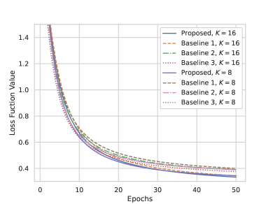
Figure 2: Loss of the MLP on the MNIST under $K=8$ and $K=16$.

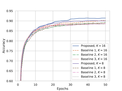
Figure 3: Accuracy of the MLP on the MNIST under $K=8$ and $K=16$.

Figs. 2 and 3 show the (testing) loss (function value) and accuracy, respectively, of the MLP on the MNIST when there are $K=8$ and $16$ subchannels. The $x$-axis indicates the global aggregations. It is seen that the FL algorithms show fast and smooth convergence within $50$ training epochs. The loss function value reaches about $0.35$, and the accuracy is about $0.92$ under OFDMA-F²L with the optimal selections. Given the number of subchannels, i.e., $K=8$ or $K=16$, OFDMA-F²L with the optimal selections outperforms the three baseline schemes with faster convergence speeds, smaller losses, and higher learning accuracies. In addition, Baseline 1 is better than Baseline 2 since Baseline 1 optimizes the client selection policy while Baseline 2 selects clients randomly. The performances of Baselines 2 and 3 are close since they each execute part of the proposed OFDMA-F²L with the optimal selections.

VI-B OFDMA-F²L on CNN Model

We also evaluate the impact of the optimal client, subchannel, and modulation selections on the learning performance (or convergence) of OFDMA-F²L on the CNN model. The CNN comprises two convolutional layers that have a kernel size of five, followed by three fully-connected layers. We train the CNN using the SGD optimizer. The ReLU units are used along with a softmax function that corresponds to ten classes for the CIFAR10 and ten digits of the FMNIST.

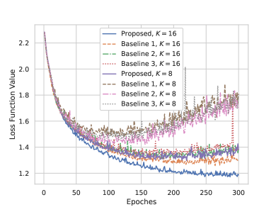
Figure 4: Loss of the CNN on the CIFAR10 under $K=8$ and $K=16$.

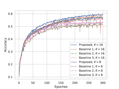
Figure 5: Accuracy of the CNN on the CIFAR10 under $K=8$ and $K=16$.

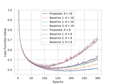
Figure 6: Loss of the CNN on the FMNIST under $K=8$ and $K=16$.

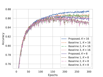
Figure 7: Accuracy of the CNN on the FMNIST under $K=8$ and $K=16$.

Figs. 4-7 show the (testing) losses and accuracies of the CNN on the CIFAR10 and FMNIST with $300$ training epochs. As the training progresses, the testing loss decreases, and the testing accuracy increases. At the beginning, the testing loss decreases rapidly, indicating that the model learns fast from the available data. Once a certain number of aggregations is reached, the rate of improvement slows down, and the testing loss converges to the minimum value, as shown in Figs. 4 and 6. Similarly, the testing accuracy increases rapidly at first, but levels off. The model reaches a plateau in its performance in Figs. 5 and 7.

It is observed in Figs. 4 and 5 that on the CIFAR10 dataset, the loss function value stabilizes around $1.2$ and the accuracy is about $0.6$ under OFDMA-F²L with the optimal selections. In contrast, the three baseline schemes yield higher loss function values and worse accuracies. In particular, when $K=8$, the (testing) losses of the three baselines first decrease and then increase as the training goes on, indicating a divergence of the model learned from the training data (or, in other words, the model incurs overfitting to the training data and does not generalize well to the testing data). This is because when $K$ is small (e.g., $K=8$), the total transmission rate is low, and the number of clients involved in the model aggregation is small, in which case, the baselines could not provide enough data for learning a good model.

It is also observed in Figs. 4 and 5 that Baseline 3 is the least stable, since it necessitates all selected clients to upload their local models simultaneously after completing the same number of iterations using Sync-FL. In this case, the global training can be significantly affected by clients with poor channels or low computing powers, especially when a large dataset is concerned.

In Figs. 6 and 7, we see that the FL algorithms are much smoother than on the CIFAR10 dataset and have faster convergence. This is because the FMNIST is a dataset of images of clothing items, which is considerably smaller compared to the CIFAR10 dataset. The images in the FMNIST dataset are also simpler and have fewer variations in color and texture, compared to the CIFAR10 images. As a result, OFDMA-F²L with the optimal selections may take a shorter time to converge to a satisfactory solution. When $K=16$, the accuracy of OFDMA-F²L with the optimal selections stabilizes at about $0.88$, while the accuracies of the three baselines are about $0.865$. In other words, OFDMA-F²L with the optimal selections has better learning performance than the baselines. When $K=8$, the (testing) loss function values of all four algorithms initially decrease and then increase during training, indicating that the models undergo overfitting. This is likely due to the low transmission rate and the limited number of clients involved in the training process, which are insufficient to capture the full complexity of the data distribution.

VI-C Performance Analysis of OFDMA-F²L

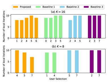
Figure 8: The number of local iterations in a selected aggregation round vs. the selected clients in the round.

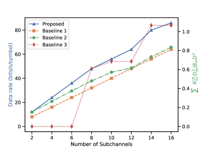
Figure 9: $\sum_{m\in{\cal M}}R^{\rm UL}_{m}\varrho_{m}^{2}/\beta_{m}$ and sum data rate vs. the number of subchannels.

Fig. 8 plots the client selection results and corresponding numbers of local iterations for each selected client at a specific training epoch of OFDMA-F²L and the other baselines when $K=8$ and $K=16$. Compared to the three baselines, more clients are selected under OFDMA-F²L with the optimal selections. Besides, OFDMA-F²L with the optimal selections accommodates more local iterations per aggregation round than the three baselines, shows a better learning performance than the baselines in Sections VI-A and VI-B. When $K=16$, Baseline 1 supports more local iterations per aggregation round than Baseline 2. When $K=8$, Baseline 1 accommodates fewer local iterations per aggregation round than Baseline 2. This is consistent with the learning performance of the three baselines presented in Sections VI-A and VI-B.

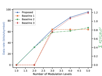
Figure 10: $\sum_{m\in{\cal M}}R^{\rm UL}_{m}D_{m}^{2}/\beta_{m}D^{2}$ and sum data rate vs. the number of modulation modes.

Figs. 9 and 10 show the objective value of problem P5 and the (uplink) sum rate of the proposed OFDMA-F²L with the optimal selections when the number of subchannels or modulation modes changes. In general, the performance metrics increase as the subchannels or modulation modes rise since the system can have a higher data rate, a shorter communication delay, and hence the lower objective function value and higher accuracy. OFDMA-F²L with the optimal selections significantly outperforms the three baselines, as the subchannels or modulations increase.

It is also observed in Fig. 9 that the objective value and data rate change linearly and synchronously with the number of subchannels under Baseline 1, as it has only two possible modulation modes. When the number of subchannels $K\leq 6$, the data rate is always zero under Baseline 3. This is because the total delay constraint cannot be satisfied with insufficient communication resources. It is further shown in Fig. 10 that when there are more than eight modulation modes, the performance of OFDMA-F²L with the optimal selections does not change, as the total power required reaches the power budget $P_{m}^{\max}$. When there are over three modulation modes, the performance of Baseline 1 stays the same since it only considers two modulation modes. In contrast, the unstable performance of Baseline 2 results from the random client selection policy. These results corroborate the merits of OFDMA-F²L with the optimal selections.

VII Conclusion

We have presented a new OFDMA-F²L framework, which allows clients to train varying numbers of iterations per aggregation round and concurrently upload their local models, thereby increasing participating clients and extending their training times. A convergence upper bound on OFDMA-F²L has been derived and minimized by jointly optimizing the selections of clients, subchannels, and modulations to maximize the weighted sum rate of the clients in each aggregation round of OFDMA-F²L. A Lagrange-dual based method has been developed to maximize the weighted sum rate, resulting in a “winner-takes-all” strategy delivering almost surely optimal selections of clients, subchannels, and modulations. As tested experimentally on MLP and CNN, OFDMA-F²L with the optimal selections can efficiently reduce communication delay, and improve the training convergence and accuracy, e.g., by about 18% and 5%, compared to its potential alternatives.

Appendix A Proof of Theorem 1

Assuming that the gradient of the global loss function is $L_{c}$-Lipschitz continuous and the first-order Taylor expansion can be conducted to obtain the upper bound of $F({\bm{\omega}}^{(\tau+1)})-F({\bm{\omega}}^{\tau})$, as provided by

$$F({\bm{\omega}}^{(\tau+1)})-F({\bm{\omega}}^{\tau}) \leq\nabla F\left({\bm{\omega}}^{\tau}\right)\left({\bm{\omega}}^{(\tau+1)}-{\bm{\omega}}^{\tau}\right)+\frac{L_{c}}{2}\left\|{\bm{\omega}}^{(\tau+1)}-{\bm{\omega}}^{\tau}\right\|^{2}.$$ (14bb)

By substituting (2) and (3) into (14bb), we have

$$F\left({\bm{\omega}}^{(\tau+1)}\right)-F\left({\bm{\omega}}^{\tau}\right) \leq-\nabla F\left({\bm{\omega}}^{\tau}\right)\sum_{m\in{\cal M}}\varrho^{\tau}_{m}\zeta^{\tau}_{m}\left(\sum^{I^{\tau}_{m}-1}_{i=0}\eta\nabla F_{m}({\bm{\omega}}^{\tau}_{m}(i))\right)$$

$$\quad+\frac{L_{c}}{2}\bigg{\|}-\sum_{m\in{\cal M}}\varrho^{\tau}_{m}\zeta^{\tau}_{m}\left(\sum^{I^{\tau}_{m}-1}_{i=0}\eta\nabla F_{m}({\bm{\omega}}^{\tau}_{m}(i))\right)\bigg{\|}^{2}$$ (14bca)

$$=\frac{\eta^{2}L_{c}}{2}\bigg{\|}\sum_{m\in{\cal M}}\varrho^{\tau}_{m}\zeta^{\tau}_{m}\left(\sum^{I^{\tau}_{m}-1}_{i=0}\nabla F_{m}({\bm{\omega}}^{\tau}_{m}(i))\right)\bigg{\|}^{2}$$

$$\quad-\eta\nabla F\left({\bm{\omega}}^{\tau}\right)\sum_{m\in{\cal M}}\varrho^{\tau}_{m}\zeta^{\tau}_{m}\left(\sum^{I^{\tau}_{m}-1}_{i=0}\nabla F_{m}({\bm{\omega}}^{\tau}_{m}(i))\right).$$ (14bcb)

We proceed by computing the expected value of both sides of (14bc) regarding ${\bm{{\cal B}}}^{\tau}$, representing the sampled mini-batches from $\cal D$ at the $\tau$-th global aggregation. It follows that

$$\mathbb{E}_{{\bm{{\cal B}}}^{\tau}}\!\left\{\!F\left({\bm{\omega}}^{(\tau+1)}\right)\right\} \leq F\left({\bm{\omega}}^{\tau}\right)-\eta\left\|\nabla F\left({\bm{\omega}}^{\tau}\right)\right\|^{2}$$ (14bd)

$$+\frac{\eta^{2}L_{c}}{2}\mathbb{E}_{{\bm{{\cal B}}}^{\tau}}\!\left\{\!\left\|\!\sum_{m\in{\cal M}}\varrho^{\tau}_{m}\zeta^{\tau}_{m}\left(\sum^{I^{\tau}_{m}-1}_{i=0}\nabla F_{m}({\bm{\omega}}^{\tau}_{m}(i);{\cal B}^{\tau}_{m}(i))\right)\right\|^{2}\!\right\}\!.$$

Since $\varrho^{\tau}_{m}=\frac{A}{I^{\tau}_{m}}\cdot\frac{D_{m}}{D}$, $\mathbb{E}_{{\bm{{\cal B}}}^{\tau}}\Big{\|}\sum_{m\in{\cal M}}\varrho^{\tau}_{m}\left(\sum^{I^{\tau}_{m}-1}_{i=0}\nabla F_{m}({\bm{\omega}}^{\tau}_{m}(i);{\cal B}^{\tau}_{m}(i))\right)\Big{\|}^{2}$ in (14bd) is rewritten as

$$\mathbb{E}_{{\bm{{\cal B}}}^{\tau}}\left\{\left\|\sum_{m\in{\cal M}}\frac{AD_{m}\zeta^{\tau}_{m}}{DI^{\tau}_{m}}\left(\sum^{I^{\tau}_{m}-1}_{i=0}\nabla F_{m}({\bm{\omega}}^{\tau}_{m}(i);{\cal B}^{\tau}_{m}(i))\right)\right\|^{2}\right\}$$ (14bea)

$$=\sum_{m\in{\cal M}}\frac{A^{2}D_{m}^{2}\zeta^{\tau}_{m}}{D^{2}}\mathbb{E}_{{{\cal B}}^{\tau}_{m}}\left\{\left\|\frac{1}{I^{\tau}_{m}}\sum^{I^{\tau}_{m}-1}_{i=0}\nabla F_{m}({\bm{\omega}}^{\tau}_{m}(i);{\cal B}^{\tau}_{m}(i))\right\|^{2}\right\}$$ (14beb)

$$=\sum_{m\in{\cal M}}\frac{A^{2}D_{m}^{2}\zeta^{\tau}_{m}}{D^{2}\left(I^{\tau}_{m}\right)^{2}}\sum^{I^{\tau}_{m}-1}_{i=0}\mathbb{E}_{{{\cal B}}^{\tau}_{m}(i)}\left\|\nabla F_{m}({\bm{\omega}}^{\tau}_{m}(i);{\cal B}^{\tau}_{m}(i))\right\|^{2}$$ (14bec)

$$\leq\sum_{m\in{\cal M}}\frac{A^{2}D_{m}^{2}\zeta^{\tau}_{m}}{D^{2}I^{\tau}_{m}}\left(\kappa_{1}+\kappa_{2}\|\nabla F(\bm{\omega}^{\tau})\|^{2}\right),$$ (14bed)

where (14beb) is due to the i.i.d. datasets of all clients; (14bec) is because the sampled mini-batches are considered to be i.i.d. between the two consecutive aggregations; and (14bed) is due to the assumption of $\mathbb{E}_{{\cal B}^{\tau}_{m}}\left\|\nabla F_{m}({\bm{\omega}}^{\tau}_{m}(i);{\cal B}^{\tau}_{m}(i))\right\|^{2}\leq\kappa_{1}+\kappa_{2}\|\nabla F(\bm{\omega}^{\tau})\|^{2},\forall m~{}\text{and}~{}\tau$.

Since $\mathbb{E}_{\bm{{\cal B}}^{\tau}}\{F({\bm{\omega}}^{\tau+1})\}=F({\bm{\omega}}^{\tau+1})$, we substitute (14be) into (14bd), yielding

$$F({\bm{\omega}}^{(\tau+1)}) \leq F({\bm{\omega}}^{\tau})-\phi_{2}\|\nabla F({\bm{\omega}}^{\tau})\|^{2}+\phi_{1},$$ (14bf)

where $\phi_{1}\triangleq\frac{\eta^{2}L_{c}}{2}\sum_{m\in{\cal M}}\frac{A^{2}\kappa_{1}D_{m}^{2}\zeta^{\tau}_{m}}{D^{2}I^{\tau}_{m}}$ and $\phi_{2}\triangleq\eta-\frac{\eta^{2}L_{c}}{2}\sum_{m\in{\cal M}}\frac{A^{2}\kappa_{2}D_{m}^{2}\zeta^{\tau}_{m}}{D^{2}I^{\tau}_{m}}$.

Detracting $F({\bm{\omega}}^{*})$ from both sides of (14bf), it follows

$$F({\bm{\omega}}^{(\tau+1)})-F({\bm{\omega}}^{*})\leq F({\bm{\omega}}^{\tau})-F({\bm{\omega}}^{*})-\phi_{2}\|\nabla F({\bm{\omega}}^{\tau})\|^{2}+\phi_{1}.$$ (14bg)

Considering Polyak-Lojasiewicz condition, we have

$$\|\nabla F({\bm{\omega}}^{\tau})\|^{2}\geq 2\rho\left(F(\bm{\omega}^{\tau})-F(\bm{\omega}^{\ast})\right).$$ (14bh)

By substituting (14bh) into (14bg), we have

$$F({\bm{\omega}}^{(\tau+1)})-F({\bm{\omega}}^{*})\leq(1-2\rho\phi_{2})\left[F({\bm{\omega}}^{\tau})-F({\bm{\omega}}^{*})\right]+\phi_{1}.$$ (14bi)

Based on (14bi), we can use mathematical induction and finally obtain

$$F({\bm{\omega}}^{\tau})-F({\bm{\omega}}^{*}) \leq\left[F({\bm{\omega}}^{0})-F({\bm{\omega}}^{*})\right]\left(1-2\rho\phi_{2}\right)^{\tau}$$ (14bj)

$$\quad+\phi_{1}\frac{1-\left(1-2\rho\phi_{2}\right)^{\tau}}{2\rho\phi_{2}},$$

which concludes this proof.

References

- [1] W. Y. B. Lim, N. C. Luong, D. T. Hoang, Y. Jiao, Y.-C. Liang, Q. Yang, D. Niyato, and C. Miao, “Federated learning in mobile edge networks: A comprehensive survey,” IEEE Commun. Surveys Tuts., vol. 22, no. 3, pp. 2031–2063, 3rd Quart. 2020.
- [2] S. Hu, X. Chen, W. Ni, E. Hossain, and X. Wang, “Distributed machine learning for wireless communication networks: Techniques, architectures, and applications,” IEEE Commun. Surveys Tuts., vol. 23, no. 3, pp. 1458–1493, 3rd Quart., 2021.
- [3] Z. Qu, S. Guo, H. Wang, B. Ye, Y. Wang, A. Y. Zomaya, and B. Tang, “Partial synchronization to accelerate federated learning over relay-assisted edge networks,” IEEE Trans. Mobile Comput., vol. 21, no. 12, pp. 4502–4516, Dec. 2022.
- [4] V.-D. Nguyen, S. K. Sharma, T. X. Vu, S. Chatzinotas, and B. Ottersten, “Efficient federated learning algorithm for resource allocation in wireless iot networks,” IEEE Internet Things J., vol. 8, no. 5, pp. 3394–3409, Mar. 2021.
- [5] J. Zhang and O. Simeone, “LAGC: Lazily aggregated gradient coding for straggler-tolerant and communication-efficient distributed learning,” IEEE Trans. Neural Netw. Learn. Syst., pp. 1–13, 2020.
- [6] Y. Ruan, X. Zhang, S.-C. Liang, and C. Joe-Wong, “Towards flexible device participation in federated learning,” in Proc. Int. Conf. Artif. Intell. Statist., vol. 130. PMLR, Apr. 2021, pp. 3403–3411.
- [7] C. Xie, S. Koyejo, and I. Gupta, “Asynchronous federated optimization,” in Annual Wrkshps Optim. Mach. Learn., 2020.
- [8] S. Yang and Y. Liu, “Training efficiency of federated learning: A wireless communication perspective,” in Proc. Int. Conf. Wireless Commun. Signal Process. (WCSP), Oct. 2020, pp. 922–926.
- [9] Q. Zeng, Y. Du, K. Huang, and K. K. Leung, “Energy-efficient radio resource allocation for federated edge learning,” in Proc. IEEE Int. Conf. Commun. Wrkshps. (ICC Wrkshps), Jun. 2020, pp. 1–6.
- [10] Y. Jiao, P. Wang, D. Niyato, B. Lin, and D. I. Kim, “Toward an automated auction framework for wireless federated learning services market,” IEEE Trans. Mobile Comput., vol. 20, no. 10, pp. 3034–3048, Oct. 2021.
- [11] J. Xu and H. Wang, “Client selection and bandwidth allocation in wireless federated learning networks: A long-term perspective,” IEEE Trans. Wireless Commun., vol. 20, no. 2, pp. 1188–1200, Feb. 2021.
- [12] X. Lin, J. Wu, J. Li, X. Zheng, and G. Li, “Friend-as-learner: Socially-driven trustworthy and efficient wireless federated edge learning,” IEEE Trans. Mobile Comput., vol. 22, no. 1, pp. 269–283, Jan. 2023.
- [13] A. Abutuleb, S. Sorour, and H. S. Hassanein, “Joint task and resource allocation for mobile edge learning,” in Proc. IEEE Globecom Conf. (GLOBECOM), Dec. 2020, pp. 1–6.
- [14] H. Chen, S. Huang, D. Zhang, M. Xiao, M. Skoglund, and H. V. Poor, “Federated learning over wireless iot networks with optimized communication and resources,” IEEE Internet of Things Journal, vol. 9, no. 17, pp. 16 592–16 605, Sep. 2022.
- [15] Z. Ji and Z. Qin, “Federated learning for distributed energy-efficient resource allocation,” in Proc. IEEE Int. Conf. Commun. (ICC), May 2022, pp. 1–6.
- [16] Z. Yang, M. Chen, W. Saad, C. S. Hong, and M. Shikh-Bahaei, “Energy efficient federated learning over wireless communication networks,” IEEE Trans. Wireless Commun., vol. 20, no. 3, pp. 1935–1949, Mar. 2021.
- [17] Y. He, M. Yang, Z. He, and M. Guizani, “Resource allocation based on digital twin-enabled federated learning framework in heterogeneous cellular network,” IEEE Trans. Veh. Tech., vol. 72, no. 1, pp. 1149–1158, Jan. 2023.
- [18] Y. Wu, Y. Song, T. Wang, L. Qian, and T. Q. S. Quek, “Non-orthogonal multiple access assisted federated learning via wireless power transfer: A cost-efficient approach,” IEEE Trans. Commun., vol. 70, no. 4, pp. 2853–2869, Apr. 2022.
- [19] M. Salehi and E. Hossain, “Federated learning in unreliable and resource-constrained cellular wireless networks,” IEEE Trans. Commun., vol. 69, no. 8, pp. 5136–5151, Aug. 2021.
- [20] Y. Chen, X. Sun, and Y. Jin, “Communication-efficient federated deep learning with layerwise asynchronous model update and temporally weighted aggregation,” IEEE Trans. Neural Netw. Learn. Syst., vol. 31, no. 10, pp. 4229–4238, Oct. 2020.
- [21] Z. Chai, Y. Chen, A. Anwar, L. Zhao, Y. Cheng, and H. Rangwala, “FedAT: A high-performance and communication-efficient federated learning system with asynchronous tiers,” in Proc. Int. Conf. High Perfor. Comput., Networking, Storage Analysis, 2021, pp. 1–17.
- [22] B. Gu, A. Xu, Z. Huo, C. Deng, and H. Huang, “Privacy-preserving asynchronous vertical federated learning algorithms for multiparty collaborative learning,” IEEE Trans. Neural Netw. Learn. Syst., vol. 33, no. 11, pp. 6103–6115, Nov. 2022.
- [23] Y. Zhang, D. Liu, M. Duan, L. Li, X. Chen, A. Ren, Y. Tan, and C. Wang, “FedMDS: An efficient model discrepancy-aware semi-asynchronous clustered federated learning framework,” IEEE Trans. Parall. Distr. Syst., vol. 34, no. 3, pp. 1007–1019, Mar. 2023.
- [24] H. Hu, Z. Salcic, L. Sun, G. Dobbie, and X. Zhang, “Source inference attacks in federated learning,” in 2021 IEEE International Conference on Data Mining (ICDM). IEEE, 2021, pp. 1102–1107.
- [25] X. Yuan, W. Ni, M. Ding, K. Wei, J. Li, and H. Vincent Poor, “Amplitude-varying perturbation for balancing privacy and utility in federated learning,” IEEE Trans. Inf. Forensics Security, vol. 18, pp. 1884–1897, 2023.
- [26] Z. Wang, Z. Zhang, Y. Tian, Q. Yang, H. Shan, W. Wang, and T. Q. S. Quek, “Asynchronous federated learning over wireless communication networks,” IEEE Trans. Wireless Commun., vol. 21, no. 9, pp. 6961–6978, Sep. 2022.
- [27] J. Liu, H. Xu, L. Wang, Y. Xu, C. Qian, J. Huang, and H. Huang, “Adaptive asynchronous federated learning in resource-constrained edge computing,” IEEE Trans. Mobile Comput., vol. 22, no. 2, pp. 674–690, Feb. 2023.
- [28] G. Zhu, Y. Wang, and K. Huang, “Broadband analog aggregation for low-latency federated edge learning,” IEEE Trans. Wireless Commun., vol. 19, no. 1, pp. 491–506, Jan. 2020.
- [29] G. Zhu, Y. Du, D. Gündüz, and K. Huang, “One-bit over-the-air aggregation for communication-efficient federated edge learning: Design and convergence analysis,” IEEE Trans. Wireless Commun., vol. 20, no. 3, pp. 2120–2135, Mar. 2021.
- [30] J. Du, B. Jiang, C. Jiang, Y. Shi, and Z. Han, “Gradient and channel aware dynamic scheduling for over-the-air computation in federated edge learning systems,” IEEE J. Sel. Areas Commun., vol. 41, no. 4, pp. 1035–1050, Apr. 2023.
- [31] C. Zhong, H. Yang, and X. Yuan, “Over-the-air federated multi-task learning over mimo multiple access channels,” IEEE Trans. Wireless Commun., vol. 22, no. 6, pp. 3853–3868, Jun. 2023.
- [32] X. Yu, B. Xiao, W. Ni, and X. Wang, “Optimal adaptive power control for over-the-air federated edge learning under fading channels,” IEEE Trans. Commun., vol. 71, no. 9, pp. 5199–5213, Sep. 2023.
- [33] B. McMahan, E. Moore, D. Ramage, S. Hampson, and B. A. y Arcas, “Communication-efficient learning of deep networks from decentralized data,” in Proc. Int. Conf. Artif. Intell. Statist. PMLR, 2017, pp. 1273–1282.
- [34] H. Viswanathan, “Capacity of Markov channels with receiver CSI and delayed feedback,” IEEE Trans. Inf. Theory, vol. 45, no. 2, pp. 761–771, 1999.
- [35] A. J. Goldsmith and S. . Chua, “Adaptive coded modulation for fading channels,” IEEE Trans. Commun., vol. 46, no. 5, pp. 595–602, 1998.
- [36] H. Malik, M. M. Alam, Y. Le Moullec, and Q. Ni, “Interference-aware radio resource allocation for 5G ultra-reliable low-latency communication,” in Proc. IEEE Globecom Workshops (GC Wkshps), 2018, pp. 1–6.
- [37] M. O’Searcoid, Metric Spaces, ser. Springer Undergraduate Mathematics Series. Springer London, 2006. [Online]. Available: https://books.google.com.au/books?id=aP37I4QWFRcC
- [38] H. Karimi, J. Nutini, and M. Schmidt, “Linear convergence of gradient and proximal-gradient methods under the Polyak-Lojasiewicz condition,” in Joint European Conference on Machine Learning and Knowledge Discovery in Databases. Springer, 2016, pp. 795–811.
- [39] T. He, X. Wang, and W. Ni, “Optimal chunk-based resource allocation for OFDMA systems with multiple BER requirements,” IEEE Trans. Veh. Technol., vol. 63, no. 9, pp. 4292–4301, 2014.
- [40] X. Yuan, S. Hu, W. Ni, R.-P. Liu, and X. Wang, “Joint user, channel, modulation-coding selection, and RIS configuration for jamming resistance in multiuser OFDMA systems,” IEEE Trans. Commun., vol. 71, no. 3, pp. 1631–1645, Mar. 2023.
- [41] S. Boyd and L. Vandenberghe, Convex Optimization. Cambridge university press, 2004.
- [42] N. Gao and X. Wang, “Optimal subcarrier-chunk scheduling for wireless OFDMA systems,” IEEE Trans. Wireless Commun., vol. 10, no. 7, pp. 2116–2123, 2011.
- [43] D. Lenz, “Singular spectrum of Lebesgue measure zero for one-dimensional quasicrystals,” Communications in mathematical physics, vol. 227, no. 1, pp. 119–130, 2002.
- [44] X. Chen, J. Cui, W. Ni, X. Wang, Y. Zhu, J. Zhang, and S. Xu, “DFT-s-OFDM: Enabling flexibility in frequency selectivity and multiuser diversity for 5G,” IEEE Consumer Electron. Mag., vol. 9, no. 6, pp. 15–22, Nov. 2020.
- [45] M. Chen, Z. Yang, W. Saad, C. Yin, H. V. Poor, and S. Cui, “A joint learning and communications framework for federated learning over wireless networks,” IEEE Trans. Wireless Commun., vol. 20, no. 1, pp. 269–283, Jan. 2021.