Factorized form of the dispersion relations of a traveling wave tube

Abstract

The traveling tube (TWT) design in a nutshell comprises of a pencil-like electron beam (e-beam) in vacuum interacting with guiding it slow-wave structure (SWS). In our prior studies the e-beam was represented by one-dimensional electron flow and SWS was represented by a transmission line (TL). We extend in this paper our previously constructed field theory for TWTs as well the celebrated Pierce theory by replacing there the standard transmission line (TL) with its generalization allowing for the low frequency cutoff. Both the standard TL and generalized transmission line (GTL) feature uniformly distributed shunt capacitance and serial inductance, but the GTL in addition to that has uniformly distributed serial capacitance. We remind the reader that the standard TL represents a waveguide operating at the so-called TEM mode with no low frequency cutoff. In contrast, the GTL represents a waveguide operating at the so-called TM mode featuring the low frequency cutoff. We develop all the details of the extended TWT field theory and using a particular choice of the TWT parameters we derive a physically appealing factorized form of the TWT dispersion relations. This form has two factors that represent exactly the dispersion functions of non-interacting GTL and the e-beam. We also find that the factorized dispersion relations comes with a number of interesting features including: (i) focus points that belong to each dispersion curve as TWT principle parameter varies; (ii) formation of “hybrid” branches of the TWT dispersion curves parts of which can be traced to non-interacting GTL and the e-beam.

I Introduction

We first review concisely the basics of traveling wave tubes. Traveling wave tube (TWT) utilizes the energy of the pencil-like electron beam (e-beam) as a flow of free electrons in a vacuum and converts it into an RF signal, see Fig. I.1. To facilitate the energy conversion and the signal amplification, the electron beam is enclosed in the so-called slow wave structure (SWS), which supports waves that are slow enough to effectively interact with the e-beam. As a result of this interaction, the kinetic energy of electrons is converted into the electromagnetic energy stored in the field, [19], Tsim [33], BBLN [3, Sec. 2.2], SchaB [28, Sec. 4]. Consequently, the key operational principle of a TWT is a positive feedback interaction between the slow-wave structure and the flow of electrons. The physical mechanism of radiation generation and its amplification is the electron bunching caused by the acceleration and deceleration of electrons along the e-beam.

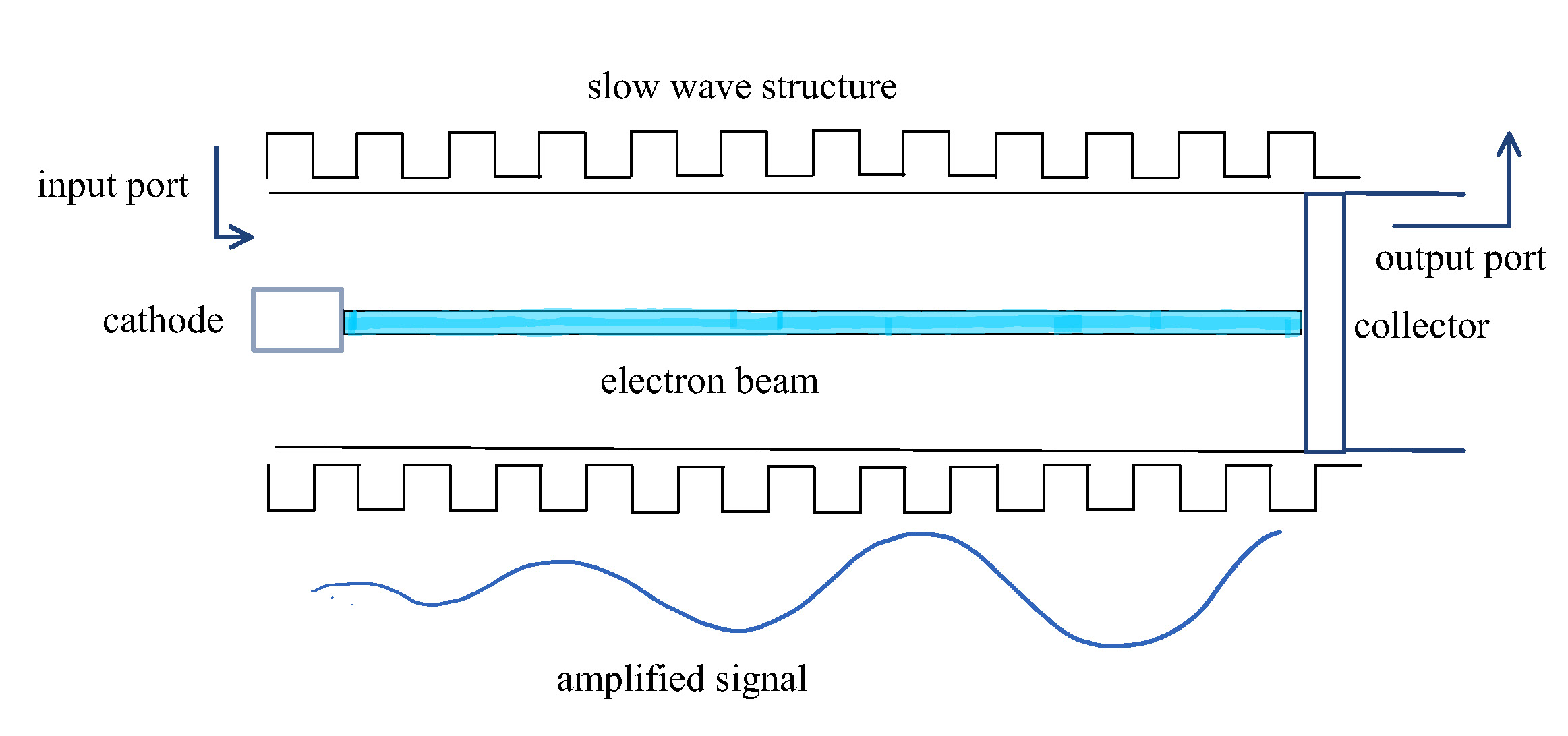
Figure I.1: The upper picture is a schematic presentation of a traveling wave tube. The lower picture shows an RF perturbation in the form of a space-charge wave that gets amplified exponentially as it propagates through the traveling wave tube.

A schematic sketch of typical TWT is shown in Fig. I.1. Such a typical TWT consists of a vacuum tube containing an e-beam that passes down the middle of an SWS such as the so-called RF circuit. It operates as follows. The left end of the RF circuit is fed with a low-powered RF signal to be amplified. The SWS electromagnetic field acts upon the e-beam causing electron bunching and the formation of the so-called space-charge wave. In turn, the electromagnetic field generated by the space charge wave induces more current back into the RF circuit with a consequent enhancement of electron bunching. As a result, the EM field is amplified as the RF signal passes down the structure until a saturation regime is reached and a large RF signal is collected at the output. The role of the SWS is to provide slow-wave modes to match up with the velocity of the electrons in the e-beam. This velocity is usually a fraction of the speed of light. Importantly, synchronism is required for an effective in-phase interaction between the SWS and the e-beam with optimal extraction of the kinetic energy of the electrons. A typical simple SWS is the helix, which reduces the speed of propagation according to its pitch. The TWT is designed so that the RF signal travels along the tube at nearly the same speed as electrons in the e-beam to facilitate effective coupling. A big picture on the flow of electrons in TWT is that they move with nearly constant velocity and loose some of their kinetic energy to the EM wave. This kind of energy transfer is observed in the Cherenkov radiation phenomenon that can be viewed then as a physical foundation for the convection instability and consequent RF signal amplification, [5, Sec. 1.1-1.2, 4.4, 4.8-4.9, 7.3, 7.6; Chap. 8].

Technical details on the designs and operation of TWTs can be found in [19], BBLN [3, Sec. 4] [27], Tsim [33]. As for a rich and interesting history of traveling wave tubes, we refer the reader to [24] and references therein.

An effective mathematical model for a TWT interacting with the e-beam was introduced by Pierce Pier51 [26, Sec. I], [27]. The celebrated Pierce model is one-dimensional; it accounts for the wave amplification, energy extraction from the e-beam and its conversion into microwave radiation in the TWT [19], [20], BBLN [3, Sec. 4], SchaB [28, Sec. 4], Tsim [33]. This model captures remarkably well significant features of the wave amplification and the beam-wave energy transfer, and is still used for basic design estimates. The Pierce theory assumes: (i) an idealized one-dimensional flow of electrons responding linearly to perturbations; (ii) a lossless transmission line (TL) representing the relevant eigenmode of the SWS that interacts with the e-beam; (iii) the TL is assumed to be spatially homogeneous with uniformly distributed shunt capacitance and serial inductance. In our paper FR [15], we have constructed a Lagrangian field theory by generalizing and extending the Pierce theory to the case of a possibly inhomogeneous MTL coupled to the e-beam. This work was extended to an analytic theory of multi-stream electron beams in traveling wave tubes in [11].

In this paper we extend first our previously constructed field theory for TWTs as well the celebrated Pierce theory by replacing there the standard transmission line (TL) with its generalization allowing for the low frequency cutoff. Both the standard TL and generalized transmission line (GTL) feature uniformly distributed shunt capacitance and serial inductance but the GTL in addition to that has uniformly distributed serial capacitance. We remind the reader that the standard TL represents a waveguide operating at the so-called TEM mode with no low frequency cutoff. In contrast, the GTL represents a waveguide operating at the so-called TM mode featuring the low frequency cutoff.

Second, using a particular choice of the TWT parameters we derive a physically appealing factorized form of the TWT dispersion relations. This form has two factors that represent exactly the dispersion functions of non-interacting GTL and the e-beam. We also find that the factorized dispersion relations imply a number of interesting features (i) focus points that belong to different dispersion curves as TWT principle parameter varies; (ii) formation of “hybrid” branches of the TWT dispersion curves parts of which can be traced to non-interacting GTL and the e-beam.

The paper is organized as follows. In Section II we review the main results of this paper. In Section III we introduce the GTL and construct the Lagrangian framework the extended analytic model for traveling wage tubes including the Euler-Lagrange field equations. In Section IV we introduce the factorized form of the dispersion relations and discuss its structure. In Section V we introduce “natural” units for our TWT theory and convert all important equations in their dimensionless form. Section VI is devoted to: (i) finding of special points as well so-called “cross-points” (at which both dispersion relations for the GTL and the e-beam are satisfied) for the TWT dispersion relations and the graphs the TWT dispersion relations; (ii) identification of a specific domain containing its graph based on the factorized of the TWT dispersion relations. In Section VII we show an exhibit of plots of the TWT dispersion curves for different values of the TWT principle parameter $\gamma$ demonstrating different topological patterns that depend on TWT parameters $\rho$ and $\chi$. In Section VIII we (i) consider a “big” picture of the TWT instabilities; (ii) introduce the concept of dispersion-instability graph and show a number of such dispersion-instability graphs demonstrating their qualitative dependence on the TWT main parameters $\gamma$, $\rho$ and $\chi$. In Section IX we consider the plots of the imaginary part $\Im\left\{k\left(\omega\right)\right\}$ of the frequency dependent dependent wavenumber $k\left(\omega\right)$ that satisfies the TWT dispersion relations. In Section X we introduce and study the “cross-point model” for the factorized dispersion relation defining a cross-point as a point $\left(k,\omega\right)$ at which the dispersion relations for the GTL and the e-beam hold simultaneously. This model is designed to demonstrate qualitative features of the TWT dispersion curve near the cross-points in the case of small coupling, that is when $\gamma\ll 1$. Finally, in Appendix we collect some additional information needed for out theoretical arguments.

Whenever possible we use figures to visualize features of our analytical developments.

II Review of main results

Leaving the detailed formulation the TWT theory including its variational Lagrangian framework to the following sections we review here concisely our main results.

The list of primary TWT parameters needed includes: (i) the GTL phase velocity $w$ in the high frequency limit; (ii) the GTL low cutoff frequency $\omega_{\mathrm{c}}$; (iii) the e-beam stationary velocity $\mathring{v}$; (iv) the so-called reduced plasma frequency $\omega_{\mathrm{rp}}$; (v) the TWT principal parameter $\gamma$ defined by, [11, 4, 24]

$$\gamma=\frac{b^{2}}{C}\frac{\sigma_{\mathrm{B}}}{4\pi}\omega_{\mathrm{rp}}^{2},$$ (II.1)

where $b$ is a dimensionless phenomenological coupling constant, and $C$ is the GTL shunt capacitance per of length and $\sigma_{\mathrm{B}}$ is the area of the cross-section of the e-beam. As formula (II.1) indicates the TWT principal parameter $\gamma$ is an integral TWT parameter. Further analysis shows that it appears naturally in factorized form of the TWT dispersion relations as a coupling parameter, and that can be explained by formula (II.1) showing that $\gamma$ is proportional to the square of the original coupling parameter $b$.

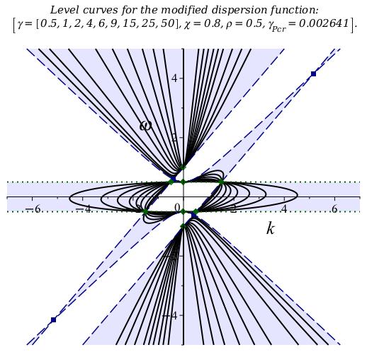
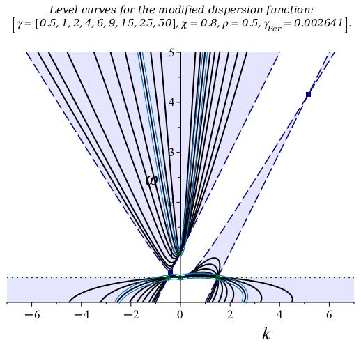
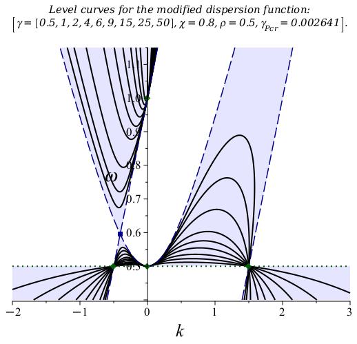
(a)                                               (b)                                               (c)

Figure II.1: Dispersion curves of the TWT dispersion relations (II.5), (II.8) for $\chi=0.8$, $\rho=0.5<1$ and $\gamma=0.5,1,2,4,6,9,15,25,50$, $\gamma_{\mathrm{Pcr}}\cong 0.002641$: (a) complete plot in the designated window; (b) a zoomed fragment of (a); (c) a zoomed fragment of (b). Solid (black) curves represent the TWT dispersion curves for indicated values of $\gamma$; dashed (blue) curves represent the dispersion curves $\mathrm{Gr}_{\mathrm{T}}$ and $\mathrm{Gr}_{\mathrm{B}}$ of non-interacting GTL and the e-beam. Shaded area identifies the dispersion domain $\mathbb{D}_{\mathrm{TB}}$, that is where $R_{\mathrm{TB}}\left(k,\omega\right)>0$. Doted (blue) horizontal straight lines represents points $\left(k,\omega_{\mathrm{c}}\right)$. Note the dispersion curves $\mathrm{Gr}_{\mathrm{TB}}\left(\gamma\right)$ pass through focal points defined by equations (II.9) marked as circle (green) dots. Square (blue) dots mark the TWT cross-points (see equations (VI.7), (VI.8)). Note also that the smaller $\gamma$ gets the closer graph $\mathrm{Gr}_{\mathrm{TB}}\left(\gamma\right)$ gets to $\mathrm{Gr}_{\mathrm{TB}}\left(0\right)=\mathrm{Gr}_{\mathrm{T}}\bigcup\mathrm{Gr}_{\mathrm{B}}$, whereas the larger $\gamma$ gets the closer graph $\mathrm{Gr}_{\mathrm{TB}}\left(\gamma\right)$ gets to $\mathrm{Gr}_{\mathrm{TB}}\left(\infty\right)$ defined by equation (VI.18).

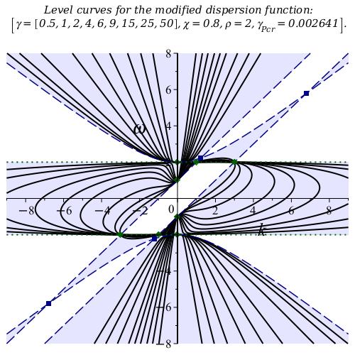
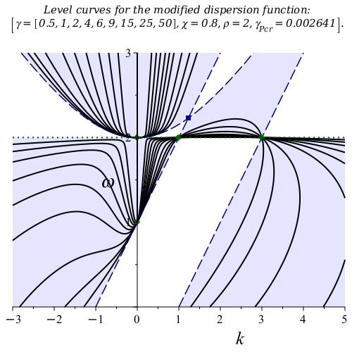
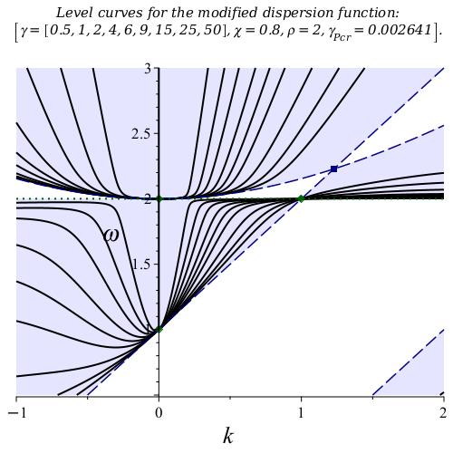
(a)                                           (b)                                           (c)

Figure II.2: Dispersion curves of the TWT dispersion relations (II.5), (II.8) for $\chi=0.8$, $\rho=2>1$ and $\gamma=0.5,1,2,4,6,9,15,25,50$, $\gamma_{\mathrm{Pcr}}\cong 0.002641$: (a) complete plot in the designated window; (b) a zoomed fragment of (a); (c) a zoomed fragment of (b). Solid (black) curves represent the TWT dispersion curves for indicated values of $\gamma$; dashed (blue) curves represent the dispersion curves of non-interacting TL and the e-beam. Shaded area identifies the dispersion domain $\mathbb{D}_{\mathrm{TB}}$, that is where $R_{\mathrm{TB}}\left(k,\omega\right)>0$. Doted (blue) horizontal straight lines represents points $\left(k,\omega_{\mathrm{c}}\right)$. Note the dispersion curves $\mathrm{Gr}_{\mathrm{TB}}\left(\gamma\right)$ pass through focal points defined by equations (II.9) marked as circle (green) dots. Square (blue) dots mark the TWT cross-points (see equations (VI.7), (VI.8)). Note also that the smaller $\gamma$ gets the closer graph $\mathrm{Gr}_{\mathrm{TB}}\left(\gamma\right)$ gets to $\mathrm{Gr}_{\mathrm{TB}}\left(0\right)=\mathrm{Gr}_{\mathrm{T}}\bigcup\mathrm{Gr}_{\mathrm{B}}$, whereas the larger $\gamma$ gets the closer graph $\mathrm{Gr}_{\mathrm{TB}}\left(\gamma\right)$ gets to $\mathrm{Gr}_{\mathrm{TB}}\left(\infty\right)$ defined by equation (VI.18).

In order to facilitate a dimensionless version of our theory we use the following three dimensionless parameters

$$\chi=\frac{w}{\mathring{v}},\quad\rho=\frac{\omega_{\mathrm{c}}}{\omega_{\mathrm{rp}}},\quad\gamma^{\prime}=\frac{\gamma}{\mathring{v}^{2}}.$$ (II.2)

We use consistently throughout this section the dimensionless settings omitting “prime” for $\gamma^{\prime}$ to have less cluttered equations.

The TWT system configuration is described by quantities $q\left(z,t\right)$ and $Q\left(z,t\right)$ which are position and time dependent charges associated with the e-beam and the GTL. They are defined as time integrals of the corresponding e-beam and GTL currents. We setup in Section III the TWT Lagrangian and obtain the Euler-Lagrange equations for $q\left(z,t\right)$ and $Q\left(z,t\right)$. We consider then the TWT system eigenmodes represented as follows:

$$Q\left(z,t\right)=\hat{Q}\left(k,\omega\right)\mathrm{e}^{-\mathrm{i}\left(\omega t-kz\right)},\quad q\left(z,t\right)=\hat{q}\left(k,\omega\right)\mathrm{e}^{-\mathrm{i}\left(\omega t-kz\right)}.$$ (II.3)

where $\omega$ and $k=k\left(\omega\right)$ are the frequency and the wavenumber, respectively. The dependence of $k\left(\omega\right)$ on the frequency $\omega$ can be found from the TWT dispersion relations analyzed in Section IV.

The Fourier transformation (see Appendix XII.1) in time $t$ and space variable $z$ of the TWT Euler-Lagrange equations can be written in the following matrix form:

$$M_{k\omega}x=0,\quad M_{k\omega}=\left[\begin{array}[]{rr}k^{2}+\frac{\rho^{2}-\omega^{2}}{\chi^{2}}&bk^{2}\\ bk^{2}&b^{2}\left[k^{2}-\frac{\left(\omega-k\right)^{2}-1}{\gamma}\right]\end{array}\right],\quad x=\left[\begin{array}[]{r}\hat{Q}\\ \hat{q}\end{array}\right].$$ (II.4)

Note that equations (II.4) can be viewed as an eigenvalue type problem for $k$ and $x$ assuming that $\omega$ and other parameters are fixed. The condition for equations (II.4) to have nontrivial nonzero solutions $x$ is $\det\left\{M_{k\omega}\right\}=0$. The later equation after algebraic transformation turns into

$$R_{\mathrm{TB}}\left(k,\omega\right)=\left[\frac{1}{k^{2}}-\frac{\chi^{2}}{\omega^{2}-\rho^{2}}\right]\left[\left(\omega-k\right)^{2}-1\right]=\gamma,$$ (II.5)

and we refer to it as the TWT dispersion relations. The TWT dispersion function $R_{\mathrm{TB}}\left(k,\omega\right)$ is evidently a rational function which is the product of two factors, namely

$$R_{\mathrm{T}}\left(k,\omega\right)\stackrel{{\scriptstyle\mathrm{def}}}{{=}}\frac{1}{k^{2}}-\frac{\chi^{2}}{\omega^{2}-\rho^{2}},\quad R_{\mathrm{B}}\left(k,\omega\right)\stackrel{{\scriptstyle\mathrm{def}}}{{=}}\left(\omega-k\right)^{2}-1,$$ (II.6)

where $R_{\mathrm{T}}\left(k,\omega\right)$ and $R_{\mathrm{B}}\left(k,\omega\right)$ are determined entirely respectively by the GTL and by the e-beam. In addition to that, if we set in equation (II.5) $\gamma=0$ we it turns into two equations:

$$R_{\mathrm{T}}\left(k,\omega\right)=\frac{1}{k^{2}}-\frac{\chi^{2}}{\omega^{2}-\rho^{2}}=0,\quad R_{\mathrm{B}}\left(k,\omega\right)=\left(\omega-k\right)^{2}-1,$$ (II.7)

which are evidently the dispersion relations of the GTL and the e-beam respectively when they do not interact. Points $\left(k,\omega\right)$ that solve simultaneously equations (II.7) are referred to as cross-points, and the exact formulas for those points are provided in Section VI.2. The cross-points are a commonly used in the TWT design since one might expect the interaction between the GTL and the e-beam to be the strongest in a vicinity of these points.

In summary, the factorized TWT dispersion relations (II.5) integrate naturally into it the dispersion relations of the non-interacting GTL and the e-beam. The TWT dispersion curves can be viewed as the “levels” of the rational function $R_{\mathrm{TB}}\left(k,\omega\right)$ determined by equation $R_{\mathrm{TB}}\left(k,\omega\right)=\gamma$.

The factorized TWT dispersion relations (II.4) can be readily recast into its polynomial form, that is

$$\left[\omega^{2}-\left(\chi^{2}k^{2}+\rho^{2}\right)\right]\left[\left(k-\omega\right)^{2}-1\right]=\gamma k^{2}\left(\omega^{2}-\rho^{2}\right),$$ (II.8)

The dispersion relations in the form (II.8) are also naturally factorized.

The TWT dispersion relations (II.5), (II.8) are studied first for the case when the both $\omega$ and $k$ are real, and that leads to the conventional dispersion curves. An important consequence of the factorized form of the TWT dispersion relations (II.5), (II.8) is that in generic case $\rho\neq 1$ there are exactly eight (or 10 if the multiplicity is counted) points $\left(k,\omega\right)$ that always satisfy them:

$$\left(0,\rho\right),\quad\left(0,\rho\right),\quad\left(0,1\right),\quad\left(\rho-1,\rho\right),\quad\left(\rho+1,\rho\right),$$ (II.9)

$$\left(0,-\rho\right),\quad\left(0,-\rho\right),\quad\left(0,-1\right),\quad\left(-\left(\rho-1\right),-\rho\right),\quad\left(-\left(\rho+1\right),-\rho\right).$$

We refer to points (II.9) as focal points since for any $\gamma>0$ the corresponding TWT dispersion curve passes through these points, see Figures II.1 and II.2 and more in Section VII.

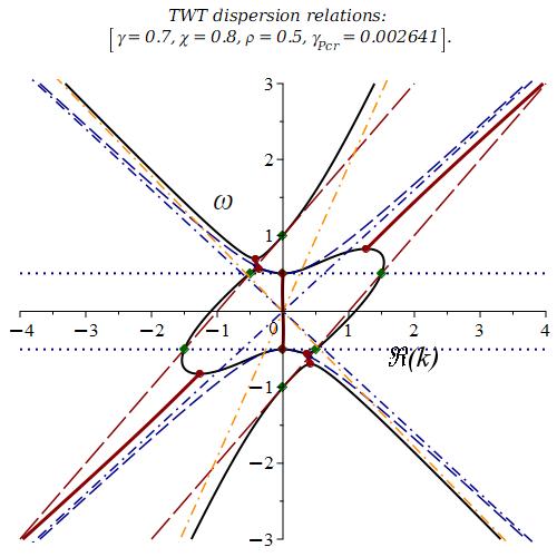
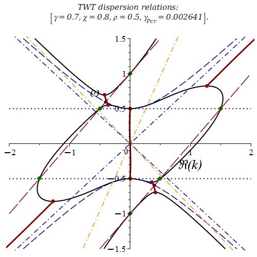
(a)                                                            (b)

Figure II.3: Dispersion-instability graph for $\chi=0.8$, $\rho=0.5<1$ and $\gamma=0.7>\gamma_{\mathrm{Pcr}}\cong 0.002641$: (a) larger version; (b) zoomed fragment of (a). Solid (black) curves represent the dispersion curves, dashed (blue) curves represent the dispersion curves for $\gamma=0$ as a reference. Dash-doted straight lines represented high frequency asymptotics for $\gamma=0.7$ (orange) and for $\gamma=0$ (blue). Doted (blue) horizontal straight lines represents points $\left(k,\pm\rho\right)$. Diamond (green) dots represent focal points defined by equations (II.9), diamond (blue) dots represent the cross-points $\mathrm{Gr}_{\mathrm{T}}\bigcap\mathrm{Gr}_{\mathrm{B}}$. The circular dots (red) identify transition to instability points (see Section VIII.1). The bold, solid (red) curves represent branches of points $\left(\Re\left\{k\right\},\omega\right)$ with real $\omega$ and $\Im\left\{k\right\}\neq 0$ which are points of the convection instability (see Section VIII.1).

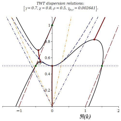
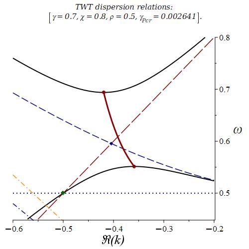
(a)                                                            (b)

Figure II.4: Zoomed fragments of the dispersion-instability graph in Fig. II.3 for $\chi=0.8$, $\rho=0.5<1$ and $\gamma=0.7>\gamma_{\mathrm{Pcr}}\cong 0.002641$: (a) zoomed fragment of Fig. II.3(b); (b) zoomed fragment of (a). Solid (black) curves represent the dispersion curves, dashed (blue) curves represent the dispersion curves for $\gamma=0$ as a reference. Dash-doted straight lines represented high frequency asymptotics for $\gamma=0.7$ (orange) and for $\gamma=0$ (blue). Doted (blue) horizontal straight lines represents points $\left(k,\pm\rho\right)$. Diamond (green) dots represent focal points defined by equations (II.9), diamond (blue) dots represent the cross-points $\mathrm{Gr}_{\mathrm{T}}\bigcap\mathrm{Gr}_{\mathrm{B}}$. The circular dots (red) identify transition to instability points (see Section VIII.1). The bold, solid (red) curves represent branches of points $\left(\Re\left\{k\right\},\omega\right)$ with real $\omega$ and $\Im\left\{k\right\}\neq 0$ which are points of the convection instability.

Fig. II.1, II.5 and II.6 show the TWT dispersion curves denoted as graphs $\mathrm{Gr}_{\mathrm{TB}}\left(\gamma\right)$. We also consider graphs $\mathrm{Gr}_{\mathrm{T}}$ and $\mathrm{Gr}_{\mathrm{B}}$ associated with dispersion equations (II.7) as natural reference frames. Graphs $\mathrm{Gr}_{\mathrm{TB}}\left(\gamma\right)$ are generated for a number of different values of $\gamma$ as the corresponding level curves for the TWT dispersion function $R_{\mathrm{TB}}\left(k,\omega\right)$. Note that all dispersion curves $\mathrm{Gr}_{\mathrm{TB}}\left(\gamma\right)$ pass through the focal points described by equations (II.9).

Figures II.3- II.6 display the TWT dispersion-instability graphs with many details described in the captions. In particular, in Figures II.5 and II.6 one can see the low and the high frequency cutoff for the convection instability that are similar to what was found in SchaFig [29] in the special case $\rho=0$.

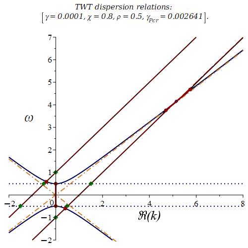
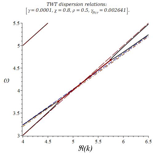
(a)                                                            (b)

Figure II.5: Dispersion-instability graph and its zoomed fragment for $\chi=0.8$, $\rho=0.5<1$ and $\gamma=0.001<\gamma_{\mathrm{Pcr}}\cong 0.002641$: (a) larger scale version; (b) zoomed fragment of (a). Solid (black) curves represent the dispersion curves, dashed (blue) curves represent the dispersion curves for $\gamma=0$ as a reference. Dash-doted straight lines represented high frequency asymptotics for $\gamma=0.7$ (orange) and for $\gamma=0$ (blue). Doted (blue) horizontal straight lines represents points $\left(k,\pm\rho\right)$. Diamond (green) dots represent focal points defined by equations (VI.1), diamond (blue) dots represent the cross-points $\mathrm{Gr}_{\mathrm{T}}\bigcap\mathrm{Gr}_{\mathrm{B}}$. The circular dots (red) identify transition to instability points (see Section VIII.1). The bold, solid (red) curves represent branches of points $\left(\Re\left\{k\right\},\omega\right)$ with real $\omega$ and $\Im\left\{k\right\}\neq 0$ which are points of the convection instability.

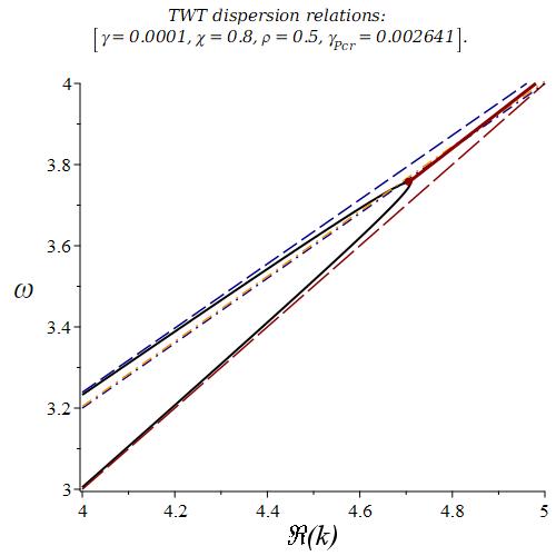
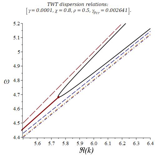
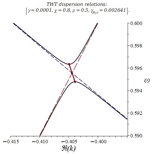
(a)                                           (b)                                           (c)

Figure II.6: Zoomed fragments of the dispersion-instability graph in Fig. II.5 for $\chi=0.8$, $\rho=0.5<1$ and $\gamma=0.001<\gamma_{\mathrm{Pcr}}\cong 0.002641$: (a) zoomed fragment of Fig. II.5(b); (b) another zoomed fragment of Fig. II.5(b); (c) zoomed fragment of Fig. II.5(a) for $\Re\left\{k\right\}<0$. Solid (black) curves represent the dispersion curves, dashed (blue) curves represent the dispersion curves for $\gamma=0$ as a reference. Dash-doted straight lines represented high frequency asymptotics for $\gamma=0.7$ (orange) and for $\gamma=0$ (blue). Doted (blue) horizontal straight lines represents points $\left(k,\pm\rho\right)$. Diamond (green) dots represent focal points defined by equations (VI.1), diamond (blue) dots represent the cross-points $\mathrm{Gr}_{\mathrm{T}}\bigcap\mathrm{Gr}_{\mathrm{B}}$. The circular dots (red) identify transition to instability points (see Section VIII.1). The bold, solid (red) curves represent branches of points $\left(\Re\left\{k\right\},\omega\right)$ with real $\omega$ and $\Im\left\{k\right\}\neq 0$ which are points of the convection instability.

We address at it is commonly done the important for TWT theory issues of instability and consequent amplification by considering complex-valued $\omega$ and $k$ solutions to the TWT dispersion relations (II.5), (II.8). More exactly, to identify two commonly studied instabilities - convective and absolute - one considers the TWT eigenmodes $f_{\omega,k}\left(z,t\right)$ of the exponential form $f_{\omega,k}\left(z,t\right)\sim\exp\left\{-\mathrm{i}\left(\omega t-kz\right)\right\}$ where possibly complex-valued $\omega$ and $k$ must satisfy the TWT dispersion relations (II.5), (II.8). In the case when $\omega$ is real and $\Im\left(k\right)\neq 0$ function $\left|f_{\omega k}\left(z,t\right)\right|$ grows or decays exponentially if $z\rightarrow\pm\infty$ and we refer to this situation as convection instability associated with amplification regimes. In the case $k$ is real but $\Im\left(\omega\right)\neq 0$ function $\left|f_{\omega k}\left(z,t\right)\right|$ grows or decays exponentially if $t\rightarrow\pm\infty$ and we refer to this situation as absolute instability associated with (exponentially growing) oscillations regimes. We focus mostly on the case of the convection instability. See Section VIII for more details.

The conventional plot of the TWT dispersion relation as shown in Fig. II.1 represents real-valued $\omega$ and $k$ that satisfies the TWT dispersion relations (II.5), (II.8). To help to visualize at least partly also the complex-valued valued solutions associated with instabilities we use the concept of dispersion-instability graph (plot) that we have developed in FigTWTbk [11, Chap. 7]. In a nutshell in the case of the convection instability, when $\omega$ is real and $k$ is complex-valued, we consider a solution $\left(k,\omega\right)$ to the TWT dispersion relations (II.5), (II.8) assuming that $k=k\left(\omega\right)$ and depict it as point $\left(\Re\left\{k\left(\omega\right)\right\},\omega\right)$ in $k\omega$-plane.

To distinguish graphically points $\left(k\left(\omega\right),\omega\right)$ associated with oscillatory modes when $k\left(\omega\right)$ is real-valued from points $\left(\Re\left\{k\left(\omega\right)\right\},\omega\right)$ associated with unstable modes when $k\left(\omega\right)$ is complex-valued with $\Im\left\{k\left(\omega\right)\right\}\neq 0$ we show points $\Im\left\{k\left(\omega\right)\right\}=0$ in black color whereas points with $\Im\left\{k\left(\omega\right)\right\}\neq 0$ are shown in red color. The corresponding curves are shown respectively as the solid (black) and solid (red) curves. We remind that every point $\left(\Re\left\{k\left(\omega\right)\right\},\omega\right)$ with $\Im\left\{k\left(\omega\right)\right\}\neq 0$ represents exactly two complex conjugate convectively unstable modes associated with $\pm\Im\left\{k\left(\omega\right)\right\}$.

Similarly, in the case of the absolute instability, when $k$ is real and $\omega$ is complex-valued, the corresponding solution $\left(k,\omega\right)$ to the TWT dispersion relations (II.4), (II.8) is depicted as point $\left(k,\Re\left\{\omega\left(k\right)\right\}\right)$ in $k\omega$-plane. To distinguish graphically points $\left(k,\omega\left(k\right)\right)$ associated with oscillatory modes when $\omega\left(k\right)$ is real-valued from points $\left(k,\Re\left\{\omega\left(k\right)\right\}\right)$ associated with absolutely unstable modes when $\omega\left(k\right)$ is complex-valued with $\Im\left\{\omega\left(k\right)\right\}\neq 0$ we show points with $\Im\left\{\omega\left(k\right)\right\}=0$ in in black color whereas points with $\Im\left\{\omega\left(k\right)\right\}\neq 0$ are shown in green color.

Fig. II.7 shows the plot shows the imaginary part $\Im\left\{k\right\}$ of the wavenumber $k=k\left(\omega\right)$ as a function of frequency $\omega$ for the selected values of the TWT parameters.

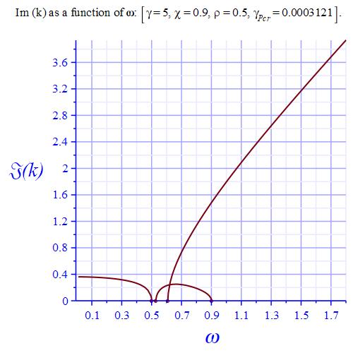
Figure II.7: The plot shows the imaginary part $\Im\left\{k\right\}$ of the wavenumber $k=k\left(\omega\right)$ as a function of frequency $\omega$ for $\gamma=5\gg\gamma_{\mathrm{Pcr}}\cong 0.0003121$, $\chi=0.9<1$ and $\rho=0.5$. Diamond square dots (red) on the $\omega$-axis mark the location of the low and the high frequency cutoffs. Note that in the case there is no high frequency cutoff.

III An extended analytic model of the traveling wave tube

We extend here an analytic model of traveling wave tube introduced and studied in our monograph [11, 4, 24]. This extended analytic model of TWT features a generalized transmission line (GTL) that can have a non-zero low frequency cutoff. More precisely, this model represents an ideal TWT as a system of a single-stream electron beam coupled to the GTL. Just as our simpler model this model is a generalization of the celebrated Pierce model [26, I], [27]. Let us start first with non-interacting e-beam and the GTL.

III.1 The non-interacting electron beam and the generalized transmission line

The main parameter describing the e-beam is the e-beam intensity

$$\beta=\frac{\sigma_{\mathrm{B}}}{4\pi}R_{\mathrm{sc}}^{2}\omega_{\mathrm{p}}^{2}=\frac{e^{2}}{m}R_{\mathrm{sc}}^{2}\sigma_{\mathrm{B}}\mathring{n},\quad\omega_{\mathrm{p}}^{2}=\frac{4\pi\mathring{n}e^{2}}{m},$$ (III.1)

where $-e$ is electron charge with $e>0$, $m$ is the electron mass, $\omega_{\mathrm{p}}$ is the e-beam plasma frequency, $\sigma_{\mathrm{B}}$ is the area of the cross-section of the e-beam, the constant $R_{\mathrm{sc}}$ is the plasma frequency reduction factor that accounts phenomenologically for finite dimensions of the e-beam cylinder as well as geometric features of the slow-wave structure, [6], [19, Sec. 9.2], BBLN [3, Sec. 3.3.3]. [11, 41, 63], and $\mathring{n}$ is the density of the number of electrons. It is assumed the electron flow of the e-beam has steady velocity $\mathring{v}>0$. Another important parameter related to e-beam when it interacts with containing it waveguide slow-wave structure is the so-called reduced plasma frequency, [19, 9.2], [7, Sec. 11.3.1]

$$\omega_{\mathrm{rp}}=R_{\mathrm{sc}}\omega_{\mathrm{p}},\quad\omega_{\mathrm{p}}^{2}=\frac{4\pi\mathring{n}e^{2}}{m}.$$ (III.2)

Note that the the interaction between the GTL and e-beam modifies the features of the e-beam by reducing the conventional plasma frequency $\omega_{\mathrm{p}}$ to the reduced plasma frequency $\omega_{\mathrm{rp}}$, and this reduction can be significant, [7, Sec. 11.3.1]. Equations (III.8) and (III.9) readily imply

$$\beta=\frac{\sigma_{\mathrm{B}}}{4\pi}\omega_{\mathrm{rp}}^{2},\quad\omega_{\mathrm{rp}}^{2}=R_{\mathrm{sc}}^{2}\frac{4\pi\mathring{n}e^{2}}{m}.$$ (III.3)

We would like to point out that there are two spatial scales related to the e-beam. The first one is

$$\lambda_{\mathrm{rp}}=\frac{2\pi\mathring{v}}{\omega_{\mathrm{rp}}},\quad\omega_{\mathrm{rp}}=R_{\mathrm{sc}}\omega_{\mathrm{p}}=R_{\mathrm{sc}}\sqrt{\frac{4\pi\mathring{n}e^{2}}{m}},$$ (III.4)

which is the distance passed by an electron for the time period $\frac{2\pi}{\omega_{\mathrm{rp}}}$ associated with the plasma oscillations at the reduced plasma frequency $\omega_{\mathrm{rp}}$. This scale is well known in the theory of klystrons and is referred to as the electron plasma wavelength, [19, 9.2], FigMCK [13]. Another spatial scale related to the e-beam that arises in our analysis is, FigCCTW [14]

$$g_{\mathrm{B}}=\frac{\sigma_{\mathrm{B}}}{4\lambda_{\mathrm{rp}}},$$ (III.5)

and we will refer to it as e-beam spatial scale.

Let us turn now to the GTL. We remind the reader that the standard transmission line (TL) has two important parameters: (i) (distributed) shunt capacitance $C>0$ per unit of length and (ii) (distributed) inductance $L>0$ per unit of length. It is well known that there are two important physical quantities phase associated with such a TL: (i) the phase velocity $w$ and (ii) the characteristic impedance $Z_{0}$ defined by the following equality, Franc [18, Sec. 7.2], MiaMaf [22, Chap. 4.2], Chip [8, Chap. 4, 5], Pain 25, Sec. 7:

$$w\stackrel{{\scriptstyle\mathrm{def}}}{{=}}\frac{1}{\sqrt{CL}},\quad Z_{0}\stackrel{{\scriptstyle\mathrm{def}}}{{=}}\sqrt{\frac{L}{C}}.$$ (III.6)

It is also known that the regular TL represents the so-called TEM mode.

To obtain a model of a wave-guided structure featuring a non-zero low frequency cutoff $\omega_{\mathrm{c}}$ one can extend the standard TL by adding to it the distributed serial capacitance $C_{\mathrm{c}}$ per unit of length, MilSchw [23, Sec. 5.1, Fig. 5.2]. The subindex “$\mathrm{c}$” in $C_{\mathrm{c}}$ is to remind that this serial capacitance is an origin of the low frequency cutoff. We refer to this extension of the standard TL as generalized transmission line (GTL). We introduce also GTL cutoff wave number $k_{\mathrm{c}}$ and the corresponding GTL cutoff frequency $\omega_{\mathrm{c}}$by the following formulas

$$k_{\mathrm{c}}\stackrel{{\scriptstyle\mathrm{def}}}{{=}}\sqrt{\frac{C}{C_{\mathrm{c}}}},\quad\omega_{\mathrm{c}}\stackrel{{\scriptstyle\mathrm{def}}}{{=}}wk_{\mathrm{c}}=w\sqrt{\frac{C}{C_{\mathrm{c}}}}=\frac{1}{\sqrt{C_{\mathrm{c}}L}}.$$ (III.7)

We use the Gaussian system of units of the physical dimensions. For the reader’s convenience we collect (i) all significant parameters related to the e-beam and the GTL and (ii) the relevant “natural” units in Tables III.1, III.2 and III.3.

$i$	current	$\frac{\left[\text{charge}\right]}{\left[\text{time}\right]}$
$q$	charge	$\left[\text{charge}\right]$
$\mathring{n}$	number of electrons p/u of volume	$\frac{\left[\text{1}\right]}{\left[\text{length}\right]^{3}}$
$\lambda_{\mathrm{rp}}=\frac{2\pi\mathring{v}}{\omega_{\mathrm{rp}}},\>\omega_{\mathrm{rp}}=R_{\mathrm{sc}}\omega_{\mathrm{p}}$	the electron plasma wavelength	$\left[\text{length}\right]$
$g_{\mathrm{B}}=\frac{\sigma_{\mathrm{B}}}{4\lambda_{\mathrm{rp}}}$	the e-beam spatial scale	$\left[\text{length}\right]$
$\beta=\frac{\sigma_{\mathrm{B}}}{4\pi}R_{\mathrm{sc}}^{2}\omega_{\mathrm{p}}^{2}=\frac{e^{2}}{m}R_{\mathrm{sc}}^{2}\sigma_{\mathrm{B}}\mathring{n}$	e-beam intensity	$\frac{\left[\text{length}\right]^{2}}{\left[\text{time}\right]^{2}}$

Table III.1: Physical dimensions of the e-beam parameters. Abbreviations: dimensionless – dim-less, p/u – per unit.

Frequency	Reduced plasma frequency	$\omega_{\mathrm{rp}}=R_{\mathrm{sc}}\omega_{\mathrm{p}}=R_{\mathrm{sc}}\sqrt{\frac{4\pi\mathring{n}e^{2}}{m}}$	$\frac{1}{\left[\text{time}\right]}$
Velocity	e-beam velocity	$\mathring{v}$	$\frac{\left[\text{length}\right]}{\left[\text{time}\right]}$
Wavenumber	Plasma oscillations wavenumber	$k_{\mathrm{rp}}=\frac{\omega_{\mathrm{rp}}}{\mathring{v}}=\frac{R_{\mathrm{sc}}\omega_{\mathrm{p}}}{\mathring{v}}$	$\frac{1}{\left[\text{length}\right]}$
Length	Plasma oscillations wavelength	$\lambda_{\mathrm{rp}}=\frac{2\pi}{k_{\mathrm{rp}}}=\frac{2\pi\mathring{v}}{\omega_{\mathrm{rp}}}$	$\left[\text{length}\right]$
Time	Plasma oscillations time period	$\tau_{\mathrm{rp}}=\frac{2\pi}{\omega_{\mathrm{rp}}}$	$\left[\text{time}\right]$

Table III.2: Natural units relevant to the e-beam parameters.

$I$	Current	$\frac{\left[\text{charge}\right]}{\left[\text{time}\right]}$
$Q$	Charge	$\left[\text{charge}\right]$
$C$	Shunt capacitance p/u of length	$\left[\text{dim-less}\right]$
$C_{\mathrm{c}}$	Serial capacitance p/u of length	$\left[\text{length}\right]^{2}$
$L$	Series inductance p/u of length	$\frac{\left[\text{time}\right]^{2}}{\left[\text{length}\right]^{2}}$
$w=\frac{1}{\sqrt{CL}}$	TL phase velocity	$\frac{\left[\text{length}\right]}{\left[\text{time}\right]}$
$k_{\mathrm{c}}=\sqrt{\frac{C}{C_{\mathrm{c}}}}$	GTL cutoff wavenumber	$\frac{1}{\left[\text{length}\right]}$
$\omega_{\mathrm{c}}=wk_{\mathrm{c}}=\frac{1}{\sqrt{C_{\mathrm{c}}L}}$	GTL cutoff frequency	$\frac{1}{\left[\text{time}\right]}$

Table III.3: Physical dimensions of the GTL related quantities. Abbreviations: dimensionless – dim-less, p/u – per unit.

The e-beam featuring space-charge effects has the following Lagrangian, [11, Chap. 24]

$$\mathcal{L}_{\mathrm{B}}=\frac{1}{2\beta}\left(\partial_{t}q+\mathring{v}\partial_{z}q\right)^{2}-\frac{2\pi}{\sigma_{\mathrm{B}}}q^{2}$$ (III.8)

whereas the GTL Lagrangian is

$$\mathcal{L}_{\mathrm{T}}=\frac{L}{2}\left(\partial_{t}Q\right)^{2}-\frac{1}{2C}\left(\partial_{z}Q\right)^{2}-\frac{1}{2C_{\mathrm{c}}}Q^{2},$$ (III.9)

where $q\left(z,t\right)$ and $Q\left(z,t\right)$ are position and time dependent charges associated with the e-beam and the GTL. They are defined as time integrals of the corresponding e-beam current $i(z,t)$ and the GTL current $I(z,t)$, that is

$$q(z,t)=\int^{t}i(z,t^{\prime})\,\mathrm{d}t^{\prime},\quad.Q(z,t)=\int^{t}I(z,t^{\prime})\,\mathrm{d}t^{\prime}.$$ (III.10)

Note the GTL Lagrangian $\mathcal{L}_{\mathrm{T}}$ defined by equation (III.9) has term $\frac{1}{2C_{\mathrm{c}}}Q^{2}$ that accounts for the energy stored in the GTL serial capacitance. This term has been added up to the TL Lagrangian introduced in [11, Chap. 24]. Note also that parameters $C$ and $C_{\mathrm{c}}$ representing respectively the shunt and the serial capacitances for the TL have different dimensions, namely the following identity holds for their dimensions: $\left[\frac{C}{C_{\mathrm{c}}}\right]=\left[\mathrm{L}^{2}\right]$ where $\mathrm{L}$ represents “length”.

The Euler-Lagrange (EL) equations corresponding to Lagrangians (III.8) and (III.9) are the following second-order differential equations:

$$L\partial_{t}^{2}Q-\frac{1}{C}\partial_{z}^{2}Q+\frac{1}{C_{\mathrm{c}}}Q=0,$$ (III.11)

$$\frac{1}{\beta}\left(\partial_{t}+\mathring{v}\partial_{z}\right)^{2}q+\frac{4\pi}{\sigma_{\mathrm{B}}}q=0,\quad\beta=\frac{\sigma_{\mathrm{B}}}{4\pi}\omega_{\mathrm{rp}}^{2}.$$ (III.12)

The Fourier transformation (see Section XII.1) in time $t$ and space variable $z$ of equations (III.11) and (III.12) yields

$$\left(\frac{k^{2}}{C}-\omega^{2}L+\frac{1}{C_{\mathrm{c}}}\right)\hat{Q}=0,\quad\frac{4\pi}{\sigma_{\mathrm{B}}}\left[1-\frac{\left(\omega-\mathring{v}k\right)^{2}}{\omega_{\mathrm{rp}}^{2}}\right]\hat{q}=0,$$ (III.13)

where $\omega$ and $k=k\left(\omega\right)$ are the frequency and the wavenumber, respectively, and functions $\hat{Q}=\hat{Q}\left(\omega,k\right)$ and $\hat{q}=\hat{q}\left(\omega,k\right)$ are the Fourier transforms of the system vector variables $Q\left(t,z\right)$ and $q\left(t,z\right)$, see Appendix XII.1.

Assuming $\hat{Q}$ and $\hat{q}$ in respective equations (III.13) to be non-zero we immediately obtain the dispersion relations for the GTL and the e-beam, namely

$$\omega=\omega_{\mathrm{T}}\left(k\right)=\pm\sqrt{w^{2}k^{2}+\omega_{\mathrm{c}}^{2}},\quad\omega=\omega_{\mathrm{B}}\left(k\right)=\mathring{v}k\pm\omega_{\mathrm{rp}}.$$ (III.14)

Then the corresponding GTL phase velocity $u_{\mathrm{T}}$ and the e-beam phase velocity $u_{\mathrm{B}}$ are

$$u=u_{\mathrm{T}}\left(\omega\right)=\pm\frac{\omega w}{\sqrt{\omega^{2}-\omega_{\mathrm{c}}^{2}}},\quad u=u_{\mathrm{B}}\left(\omega\right)=\frac{\mathring{v}\omega}{\omega\pm\omega_{\mathrm{rp}}},$$ (III.15)

The equations (III.14), (III.15) imply the following asymptotic formulas for $\omega_{\mathrm{T}}\left(k\right)$ and $u_{\mathrm{T}}\left(\omega\right)$:

$$\omega=\omega_{\mathrm{T}}\left(k\right)=\pm\left[wk+\frac{\omega_{\mathrm{c}}^{2}}{2wk}-\frac{\omega_{\mathrm{c}}^{4}}{8\left(wk\right)^{3}}+\frac{\omega_{\mathrm{c}}^{6}}{16\left(wk\right)^{5}}+O\left(\frac{1}{k^{7}}\right)\right],\quad k\rightarrow\infty,$$ (III.16)

$$u=u_{\mathrm{T}}\left(\omega\right)=w\left[1+\frac{\omega_{\mathrm{c}}^{2}}{2\omega^{2}}+\frac{3\omega_{\mathrm{c}}^{4}}{8\omega^{4}}+\frac{5\omega_{\mathrm{c}}^{6}}{16\omega^{6}}+O\left(\frac{1}{\omega^{8}}\right)\right],\quad\omega\rightarrow\infty.$$ (III.17)

In particular, it follows from equation (III.17) that

$$\lim_{\omega\rightarrow\infty}u_{\mathrm{T}}\left(\omega\right)=\pm w=\pm\frac{1}{\sqrt{CL}}.$$ (III.18)

Equations (III.16)-(III.18) indicate that at high frequency and wavenumbers the difference between the TL and the GTL becomes negligibly small.

III.2 The TWT Lagrangian and the evolution equations

The TWT-system Lagrangian $\mathcal{L}{}_{\mathrm{TB}}$ is defined similarly to its expression in [11, 4, 24] with the only difference that there is an additional term related to serial capacitance $C_{\mathrm{c}}$ as in equation (III.9), namely

$$\mathcal{L}{}_{\mathrm{TB}}=\mathcal{L}_{\mathrm{B}}+\mathcal{L}_{\mathrm{Tb}},\;\mathcal{L}_{\mathrm{B}}=\frac{1}{2\beta}\left(\partial_{t}q+\mathring{v}\partial_{z}q\right)^{2}-\frac{2\pi}{\sigma_{\mathrm{B}}}q^{2},$$ (III.19)

$$\mathcal{L}_{\mathrm{Tb}}=\frac{L}{2}\left(\partial_{t}Q\right)^{2}-\frac{1}{2C}\left(\partial_{z}Q+b\partial_{z}q\right)^{2}-\frac{1}{2C_{\mathrm{c}}}Q^{2},$$

where $b$ is the so-called coupling constant which is a dimensionless phenomenological parameter and other parameters are discussed in Section III.1. Constant $b$ is assumed often to satisfy $0<b\leq 1$ effectively reducing the inductive input of the e-beam current into the shunt current, see FigTWTbk [11, Chap. 3] for more details. Note that coupling between the GTL and e-beam is introduced through term $-\frac{1}{2C}\left(\partial_{z}Q+b\partial_{z}q\right)^{2}$indicating that the GTL distributed shunt capacitance $C$ is shared with e-beam. Following to developments in [11, 4, 24] as well equations (III.3) we introduce the TWT principal parameter $\gamma$ defined by

$$\gamma=\frac{b^{2}}{C}\beta=\frac{b^{2}}{C}\frac{\sigma_{\mathrm{B}}}{4\pi}\omega_{\mathrm{rp}}^{2},\quad\omega_{\mathrm{rp}}^{2}=R_{\mathrm{sc}}^{2}\frac{4\pi\mathring{n}e^{2}}{m}.$$ (III.20)

The Euler-Lagrange (EL) equations corresponding to the Lagrangian $\mathcal{L}{}_{\mathrm{TB}}$ defined by equations (III.19) are the following system of the second-order differential equations

$$L\partial_{t}^{2}Q-\frac{1}{C}\partial_{z}^{2}\left(Q+bq\right)+\frac{1}{C_{\mathrm{c}}}Q^{2}=0,$$ (III.21)

$$\frac{1}{\beta}\left(\partial_{t}+\mathring{v}\partial_{z}\right)^{2}q+\frac{4\pi}{\sigma_{\mathrm{B}}}q-\frac{b}{C}\partial_{z}^{2}\left(Q+bq\right)=0,\quad\beta=\frac{\sigma_{\mathrm{B}}}{4\pi}\omega_{\mathrm{rp}}^{2}.$$ (III.22)

The Fourier transformation (see Appendix XII.1) in time $t$ and space variable $z$ of equations (III.21) and (III.22) yields

$$\left(\frac{k^{2}}{C}-\omega^{2}L+\frac{1}{C_{\mathrm{c}}}\right)\hat{Q}+k^{2}\frac{b}{C}\hat{q}=0,$$ (III.23)

$$\frac{bk^{2}}{C}\hat{Q}+\left\{\frac{b^{2}k^{2}}{C}+\frac{4\pi}{\sigma_{\mathrm{B}}}\left[1-\frac{\left(\omega-\mathring{v}k\right)^{2}}{\omega_{\mathrm{rp}}^{2}}\right]\right\}\hat{q}=0,$$ (III.24)

where functions $\hat{Q}=\hat{Q}\left(k,\omega\right)$ and $\hat{q}=\hat{q}\left(k,\omega\right)$ are the Fourier transforms of the system variables $Q\left(t,z\right)$ and $q\left(t,z\right)$. We will refer to equations (III.23), (III.24) as transformed EL equations. The TWT-system eigenmodes are naturally assumed to be of the form

$$Q\left(z,t\right)=\hat{Q}\left(k,\omega\right)\mathrm{e}^{-\mathrm{i}\left(\omega t-kz\right)},\quad q\left(z,t\right)=\hat{q}\left(k,\omega\right)\mathrm{e}^{-\mathrm{i}\left(\omega t-kz\right)},$$ (III.25)

where $\omega$ and $k=k\left(\omega\right)$ are the frequency and the wavenumber, respectively. The dependence of $k\left(\omega\right)$ on the frequency $\omega$ can be found from the TWT dispersion relations analyzed in Section IV.

Multiplying the EL equations (III.23), (III.24) by $C$ we can recast them into the following matrix form:

$$M_{k\omega}x=0,\quad M_{k\omega}=\left[\begin{array}[]{rr}k^{2}-\frac{\omega^{2}}{w^{2}}+\frac{C}{C_{\mathrm{c}}}&bk^{2}\\ bk^{2}&b^{2}k^{2}+\frac{4\pi C}{\sigma_{\mathrm{B}}}\left[1-\frac{\left(\omega-\mathring{v}k\right)^{2}}{\omega_{\mathrm{rp}}^{2}}\right]\end{array}\right],\quad x=\left[\begin{array}[]{r}\hat{Q}\\ \hat{q}\end{array}\right].$$ (III.26)

Note that equations (III.26) can be viewed as an eigenvalue type problem for $k$ and $x$ assuming that $\omega$ and other parameters are fixed.

Taking into account expressions (III.6), (III.6) for $w$ and $\omega_{\mathrm{c}}$ as well as expression (III.20) for the TWT principle parameter $\gamma$ we can rewrite equations (III.26) as

$$M_{k\omega}x=0,\quad M_{k\omega}=M_{k\omega}\left(b\right)=\left[\begin{array}[]{rr}k^{2}+\frac{\omega_{\mathrm{c}}^{2}-\omega^{2}}{w^{2}}&bk^{2}\\ bk^{2}&b^{2}\left[k^{2}+\frac{\omega_{\mathrm{rp}}^{2}-\left(\omega-\mathring{v}k\right)^{2}}{\gamma}\right]\end{array}\right],\quad x=\left[\begin{array}[]{r}\hat{Q}\\ \hat{q}\end{array}\right].$$ (III.27)

Yet another equivalent form of equations (III.27) can be obtained by using phase velocity $u=\frac{\omega}{k}$ instead of wavenumber $k$ in equation (III.27), namely

$$M_{u\omega}x=0,\quad M_{u\omega}=M_{u\omega}\left(b\right)=\left[\begin{array}[]{rr}\frac{\omega^{2}}{u^{2}}+\frac{\omega_{\mathrm{c}}^{2}-\omega^{2}}{w^{2}}&\frac{b\omega^{2}}{u^{2}}\\ \frac{b\omega^{2}}{u^{2}}&\left[\frac{\omega^{2}}{u^{2}}+\frac{1}{\gamma}\left(\omega_{\mathrm{rp}}^{2}-\frac{\omega^{2}\left(u-\mathring{v}\right)^{2}}{u^{2}}\right)\right]b^{2}\end{array}\right],\quad x=\left[\begin{array}[]{r}\hat{Q}\\ \hat{q}\end{array}\right],$$ (III.32)

where we use once again the principal TWT parameter $\gamma=\frac{b^{2}}{C}\beta=\frac{b^{2}}{C}\frac{\sigma_{\mathrm{B}}}{4\pi}\omega_{\mathrm{rp}}^{2}$ defined by equations (III.20).

Note that matrices $M_{k\omega}\left(b\right)$ and $M_{u\omega}\left(b\right)$ satisfy the following factorized representations

$$M_{k\omega}\left(b\right)=D_{b}M_{k\omega}\left(1\right)D_{b},\quad M_{u\omega}\left(b\right)=D_{b}M_{u\omega}\left(1\right)D_{b}\quad D_{b}=\left[\begin{array}[]{rr}1&0\\ 0&b\end{array}\right],$$ (III.33)

where matrices $M_{k\omega}\left(1\right)$ and $M_{u\omega}\left(1\right)$ evidently do not depend on $b$.

IV The dispersion relations in factorized form

As it was already mentioned the matrix form of the EL equations (III.27) and (III.32) can be viewed as a kind of eigenvalue problem for $k$ and $u$ with other involved parameters including frequency $\omega$ considered as being fixed. The condition for these equations to have nontrivial nonzero solutions $x$ is that the determinants of matrices $M_{k\omega}$ and $M_{u\omega}$ defined respectively by equations (III.27) and (III.32) must be zero, that is

$$\det\left\{M_{k\omega}\right\}=0,\quad\det\left\{M_{u\omega}\right\}=0.$$ (IV.1)

Equations (IV.1) establish relations between $k$ or $u$ and $\omega$ and consequently they can be viewed respectively as the dispersion relation or the velocity dispersion relation. After tedious algebraic transformations equations (IV.1) can be turned respectively into the following factorized forms:

$$\left[\frac{1}{k^{2}}-\frac{w^{2}}{\omega^{2}-\omega_{\mathrm{c}}^{2}}\right]\left[\left(\omega-\mathring{v}k\right)^{2}-\omega_{\mathrm{rp}}^{2}\right]=\gamma,\quad\gamma=\frac{b^{2}}{C}\frac{\sigma_{\mathrm{B}}}{4\pi}\omega_{\mathrm{rp}}^{2}$$ (IV.2)

$$\left[u^{2}-\frac{w^{2}\omega^{2}}{\omega^{2}-\omega_{\mathrm{c}}^{2}}\right]\left[\frac{\left(u-\mathring{v}\right)^{2}}{u^{2}}-\frac{\omega_{\mathrm{rp}}^{2}}{\omega^{2}}\right]=\gamma,\quad u=\frac{\omega}{k}.$$ (IV.3)

We refer to equations (IV.2) and (IV.3) respectively as the factorized form of the TWT dispersion relations and the TWT velocity dispersion relations. These equations suggest a natural interpretation of the TWT principle parameter $\gamma$ as a coupling parameter between GTL and the e-beam. Note that equations (IV.2) and (IV.3) do not involve parameter $b$ explicitly but rather through the TWT principle parameter $\gamma$, and that is explained by identities (III.33).

Sometimes it is advantageous to use the following polynomial equation which is evidently equivalent to the TWT dispersion relations (IV.2):

$$\left[\omega^{2}-\left(w^{2}k^{2}+\omega_{\mathrm{c}}^{2}\right)\right]\left[\left(\omega-\mathring{v}k\right)^{2}-\omega_{\mathrm{rp}}^{2}\right]=\gamma k^{2}\left(\omega^{2}-\omega_{\mathrm{c}}^{2}\right).$$ (IV.4)

For every fixed $\omega$ equation (IV.4) is exactly forth degree polynomial equation for $k=k\left(\omega\right)$, and for every fixed $k$ equation (IV.4) is exactly forth degree polynomial equation for $\omega=\omega\left(k\right)$. The factorized form (IV.4) of the TWT dispersion relations naturally integrates into it the dispersion relations (III.14) of the GTL and the e-beam. Equation (IV.4) is instrumental for our analysis of analytical properties the TWT dispersion relations.

To emphasize the structure of the factorized form (IV.4) of the TWT dispersion relation we introduce

$$G_{\mathrm{T}}\left(k,\omega\right)\stackrel{{\scriptstyle\mathrm{def}}}{{=}}\omega^{2}-\left(w^{2}k^{2}+\omega_{\mathrm{c}}^{2}\right);\quad G_{\mathrm{B}}\left(k,\omega\right)\stackrel{{\scriptstyle\mathrm{def}}}{{=}}\left(\omega-\mathring{v}k\right)^{2}-\omega_{\mathrm{rp}}^{2};\quad G_{\mathrm{cT}}\left(k,\omega\right)\stackrel{{\scriptstyle\mathrm{def}}}{{=}}k^{2}\left(\omega^{2}-\omega_{\mathrm{c}}^{2}\right),$$ (IV.5)

where $G_{\mathrm{T}}\left(k,\omega\right)$ and $G_{\mathrm{B}}\left(k,\omega\right)$ are the dispersion functions related to respectively the GTL and the e-beam. Then the TWT dispersion relation (IV.4) can be readily recast as

$$G_{\mathrm{T}}\left(k,\omega\right)G_{\mathrm{B}}\left(k,\omega\right)=\gamma G_{\mathrm{cT}}\left(k,\omega\right),$$ (IV.6)

where $\gamma$ can be naturally interpreted as the coupling parameter and $G_{\mathrm{cT}}\left(k,\omega\right)$ as a supplementary coupling function that dependents only on the GTL through its cutoff frequency $\omega_{\mathrm{c}}$.

Using equations (IV.5) we can recast the dispersion relation in the form (IV.2) as follows

$$R_{\mathrm{TB}}\left(k,\omega\right)\stackrel{{\scriptstyle\mathrm{def}}}{{=}}\frac{G_{\mathrm{T}}\left(k,\omega\right)G_{\mathrm{B}}\left(k,\omega\right)}{G_{\mathrm{cT}}\left(k,\omega\right)}=\gamma,\quad k\neq 0,\quad\omega^{2}\neq\omega_{\mathrm{c}}^{2},$$ (IV.7)

$$R_{\mathrm{TB}}\left(k,\omega\right)=\left[\frac{1}{k^{2}}-\frac{w^{2}}{\omega^{2}-\omega_{\mathrm{c}}^{2}}\right]\left[\left(\omega-\mathring{v}k\right)^{2}-\omega_{\mathrm{rp}}^{2}\right].$$ (IV.8)

The significance of the TWT dispersion relation in the form (IV.7), (IV.8) is that its right-hand side is just a coupling constant $\gamma$. Consequently, these equations represent the TWT dispersion curves as the level curves of the factorized function $R_{\mathrm{TB}}\left(k,\omega\right)$ with its first and the second factors associated respectively with the GTL and the e-beam. In particular, the coupling parameter $\gamma$ appears in equation (IV.7) as the “level” of function $R_{\mathrm{TB}}\left(k,\omega\right)$. The factorized form (IV.8) for function $R_{\mathrm{TB}}\left(k,\omega\right)$ and equation (IV.7) demonstrate once again that parameter $\gamma$ plays a role of a coupling parameter between the GTL and the e-beam.

If we set in equation (IV.4) $\gamma=0$ the equation turns readily into the dispersion relations (IV.9) of non-interacting GTL and the e-beam, namely

$$G_{\mathrm{T}}\left(k,\omega\right)=\omega^{2}-\left(w^{2}k^{2}+\omega_{\mathrm{c}}^{2}\right)=0,\quad G_{\mathrm{B}}\left(k,\omega\right)=\left(\omega-\mathring{v}k\right)^{2}-\omega_{\mathrm{rp}}^{2}=0,\quad\gamma=0.$$ (IV.9)

It is worth noting that the dispersion relations (IV.9) for non-interacting GTL and e-beam clearly identify two natural frequency scales: (i) the cutoff frequency $\omega_{\mathrm{c}}$ associated with the GTL; (ii) the plasma frequency $\omega_{\mathrm{p}}$ associated with the e-beam.

Note also that if $\gamma\rightarrow\infty$ then dividing both sides of equation (IV.6) by $\gamma$ we obtain in the limit

$$G_{\mathrm{cT}}\left(k,\omega\right)=k^{2}\left(\omega^{2}-\omega_{\mathrm{c}}^{2}\right)=0,\quad\gamma\rightarrow\infty.$$ (IV.10)

As to the TWT velocity the dispersion relations (IV.3) we can proceed similarly to the case of the TWT dispersion relations (IV.2). We first introduce dispersion functions $F_{\mathrm{T}}\left(u\right)$ and $F_{\mathrm{B}}\left(u\right)$ corresponding respectively to the GTL and the e-beam as follows:

$$F_{\mathrm{T}}\left(u\right)\stackrel{{\scriptstyle\mathrm{def}}}{{=}}u^{2}-\frac{w^{2}\omega^{2}}{\omega^{2}-\omega_{\mathrm{c}}^{2}},\quad F_{\mathrm{B}}\left(u\right)\stackrel{{\scriptstyle\mathrm{def}}}{{=}}\frac{\left(u-\mathring{v}\right)^{2}}{u^{2}}-\frac{\omega_{\mathrm{rp}}^{2}}{\omega^{2}},\quad u=\frac{\omega}{k},$$ (IV.11)

where $u$ is the phase velocity. Then the TWT velocity dispersion relations (IV.3) takes the form

$$F_{\mathrm{T}}\left(u\right)F_{\mathrm{B}}\left(u\right)=\left[u^{2}-\frac{w^{2}\omega^{2}}{\omega^{2}-\omega_{\mathrm{c}}^{2}}\right]\left[\frac{\left(u-\mathring{v}\right)^{2}}{u^{2}}-\frac{\omega_{\mathrm{rp}}^{2}}{\omega^{2}}\right]=\gamma,\quad u=\frac{\omega}{k},$$ (IV.12)

Note for $\gamma=0$ we readily recover from the TWT velocity dispersion equation (IV.12) equations

$$F_{\mathrm{T}}\left(u\right)=u^{2}-\frac{w^{2}\omega^{2}}{\omega^{2}-\omega_{\mathrm{c}}^{2}}=0,\quad F_{\mathrm{B}}\left(u\right)=\frac{\left(u-\mathring{v}\right)^{2}}{u^{2}}-\frac{\omega_{\mathrm{rp}}^{2}}{\omega^{2}}=0,$$ (IV.13)

that match the velocity dispersion relations (III.15) for non-interacting GTL and the e-beam.

Recall that the Pierce theory emerges from our field theory as the high-frequency limit $\omega\rightarrow\infty$, FigTWTbk [11, Chap. 4.2, 29, 62]. Consequently the high-frequency limit of dispersion relations (IV.12) is

$$\left(u^{2}-w^{2}\right)\frac{\left(u-\mathring{v}\right)^{2}}{u^{2}}=\gamma,\quad u=\frac{\omega}{k},\quad\omega\rightarrow\infty,$$ (IV.14)

$$F\left(u\right)=\frac{\left(u^{2}-{\it\chi}^{2}\right)\left(u-1\right)^{2}}{u^{2}}=\gamma>0.$$ (IV.15)

which is exactly the velocity dispersion relation for the Pierce theory, FigTWTbk [11, Chap. 4.2, 29, 62].

V Dimensionless set up

We pursue here a dimensionless setup for the theory developed in previous sections. We often use symbol “prime” to indicate that we are dealing with the dimensionless version of a variable or a parameter. It is often convenient to use the following dimensionless variables and parameters, FigTWTbk [11, Chap. 3, 4, 30].

$$u^{\prime}=\frac{u}{\mathring{v}},\quad\gamma^{\prime}=\frac{\gamma}{\mathring{v}{}^{2}},\quad\omega^{\prime}=\frac{\omega}{\omega_{\mathrm{rp}}},\quad\rho\stackrel{{\scriptstyle\mathrm{def}}}{{=}}\frac{\omega}{\omega_{\mathrm{rp}}}\quad\chi\stackrel{{\scriptstyle\mathrm{def}}}{{=}}\frac{w}{\mathring{v}},$$

where when defining dimensionless parameter $\rho$ we tacitly assume that $\omega_{\mathrm{rp}}>0$. The definitions of the GTL and e-beam parameters are provided in Section III.1.

For the reader convenience expressions for dimensionless variables and dimensionless TWT parameters are collected respectively in Tables V.1 and V.2

Frequency	$\omega^{\prime}=\frac{\omega}{\omega_{\mathrm{rp}}},\quad\omega_{\mathrm{rp}}=R_{\mathrm{sc}}\omega_{\mathrm{p}},\quad\omega_{\mathrm{p}}=\sqrt{\frac{4\pi\mathring{n}e^{2}}{m}}$
Velocity	$v^{\prime}=\frac{v}{\mathring{v}}$
Wavenumber	$k^{\prime}=\frac{k}{k_{\mathrm{rp}}},\quad k_{\mathrm{rp}}=\frac{\omega_{\mathrm{rp}}}{\mathring{v}}=\frac{R_{\mathrm{sc}}\omega_{\mathrm{p}}}{\mathring{v}}$
Length	$\lambda^{\prime}=\frac{\lambda}{\lambda_{\mathrm{rp}}},\quad\lambda_{\mathrm{rp}}=\frac{2\pi}{k_{\mathrm{rp}}}=\frac{2\pi\mathring{v}}{\omega_{\mathrm{rp}}}$
Time	$t^{\prime}=\frac{t}{\tau_{\mathrm{rp}}},\quad\tau_{\mathrm{rp}}=\frac{2\pi}{\omega_{\mathrm{rp}}}$

Table V.1: Dimensionless primary variables based on the e-beam natural units, see Table III.2 .

The main dimensionless TWT parameters are collected in Table V.2.

$\chi=\frac{w}{\mathring{v}}=\frac{1}{\mathring{v}\sqrt{CL}}$	TL dim-less phase velocity
$\rho=\frac{\omega_{\mathrm{c}}}{\omega_{\mathrm{rp}}}=\frac{1}{\omega_{\mathrm{rp}}\sqrt{C_{\mathrm{c}}L}}$	GTL dimensionless cutoff frequency
$\beta^{\prime}=\frac{\beta}{\mathring{v}^{2}}=\frac{\pi\sigma_{\mathrm{B}}}{\lambda_{\mathrm{rp}}^{2}}=\frac{4\pi g_{\mathrm{B}}}{\lambda_{\mathrm{rp}}}$	dimensionless e-beam intensity
$\gamma^{\prime}=\frac{b^{2}}{C}\beta^{\prime}=\frac{b^{2}\beta}{C\mathring{v}^{2}}=\frac{b^{2}\pi\sigma_{\mathrm{B}}}{C\lambda_{\mathrm{rp}}^{2}}$	dimensionless TWT parameter

Table V.2: Dimensionless TWT variables, see Table III.1.

To avoid cluttered equations we often omit “prime” symbol when writing expressions with dimensionless variables and parameters presuming that it is clear from the context if the dimensionless variables are used. For instance, it is the case when dimensionless parameters $\chi$ and/or $\rho$ enter the relevant expressions.

The dimensionless form of equations (III.27) and (III.32) is

$$M_{k\omega}x=0,\quad M_{k\omega}=\left[\begin{array}[]{rr}k^{2}+\frac{\rho^{2}-\omega^{2}}{\chi^{2}}&bk^{2}\\ bk^{2}&b^{2}\left[k^{2}-\frac{\left(\omega-k\right)^{2}-1}{\gamma}\right]\end{array}\right],\quad x=\left[\begin{array}[]{r}\hat{Q}\\ \hat{q}\end{array}\right]$$ (V.1)

$$M_{u\omega}x=0,\quad M_{u\omega}=\left[\begin{array}[]{rr}\frac{\omega^{2}}{u^{2}}+\frac{\rho^{2}-\omega^{2}}{\chi^{2}}&\frac{b\omega^{2}}{u^{2}}\\ \frac{b\omega^{2}}{u^{2}}&\left[\frac{\omega^{2}}{u^{2}}+\frac{1}{\gamma}\left(1-\frac{\omega^{2}\left(u-1\right)^{2}}{u^{2}}\right)\right]b^{2}\end{array}\right],\quad x=\left[\begin{array}[]{r}\hat{Q}\\ \hat{q}\end{array}\right]$$ (V.2)

The dimensionless form of the TWT dispersion relations (IV.2) and (IV.4) is

$$\left[\frac{1}{k^{2}}-\frac{\chi^{2}}{\omega^{2}-\rho^{2}}\right]\left[\left(\omega-k\right)^{2}-1\right]=\gamma,$$ (V.3)

$$\left[\omega^{2}-\left(\chi^{2}k^{2}+\rho^{2}\right)\right]\left[\left(k-\omega\right)^{2}-1\right]=\gamma k^{2}\left(\omega^{2}-\rho^{2}\right),$$ (V.4)

The dimensionless form of the TWT velocity dispersion relations (IV.3) is

$$\left[u^{2}-\frac{\chi^{2}\omega^{2}}{\omega^{2}-\rho^{2}}\right]\left[\frac{\left(u-1\right)^{2}}{u^{2}}-\frac{1}{\omega^{2}}\right]=\gamma,\quad u=\frac{\omega}{k},$$ (V.5)

The dimensionless form of the TWT velocity dispersion relations (IV.14) for the Pierce theory, which is the high-frequency limit $\omega\rightarrow\infty$ of our theory, FigTWTbk [11, Chap. 4.2, 29, 62], is

$$\frac{\left(u^{2}-{\it\chi}^{2}\right)\left(u-1\right)^{2}}{u^{2}}=\gamma,\quad u=\frac{\omega}{k}.$$ (V.6)

The dimensionless form of the dispersion functions (IV.5) is

$$G_{\mathrm{T}}\left(k,\omega\right)\stackrel{{\scriptstyle\mathrm{def}}}{{=}}\omega^{2}-\left(\chi^{2}k^{2}+\rho^{2}\right);\quad G_{\mathrm{B}}\left(k,\omega\right)\stackrel{{\scriptstyle\mathrm{def}}}{{=}}\left(k-\omega\right)^{2}-1;\quad G_{\mathrm{cT}}\left(k,\omega\right)\stackrel{{\scriptstyle\mathrm{def}}}{{=}}k^{2}\left(\omega^{2}-\rho^{2}\right),$$ (V.7)

The dimensionless form of the dispersion relations (IV.9) for non-interacting GTL and the e-beam is

$$G_{\mathrm{T}}\left(k,\omega\right)=\omega^{2}-\left(\chi^{2}k^{2}+\rho^{2}\right)=0,\quad G_{\mathrm{B}}\left(k,\omega\right)=\left(k-\omega\right)^{2}-1=0,\quad\gamma=0.$$ (V.8)

Finally, the dimensionless form of the TWT dispersion relations (IV.7) and (IV.8) is

$$R_{\mathrm{TB}}\left(k,\omega\right)\stackrel{{\scriptstyle\mathrm{def}}}{{=}}\frac{G_{\mathrm{T}}\left(k,\omega\right)G_{\mathrm{B}}\left(k,\omega\right)}{G_{\mathrm{cT}}\left(k,\omega\right)}=\gamma,\quad k\neq 0,\quad\omega^{2}\neq\rho^{2},$$ (V.9)

$$R_{\mathrm{TB}}\left(k,\omega\right)=\left[\frac{1}{k^{2}}-\frac{\chi^{2}}{\omega^{2}-\rho^{2}}\right]\left[\left(k-\omega\right)^{2}-1\right].$$ (V.10)

VI Dispersion graphs and domains

In this section we introduce and study geometric and topological concepts related to the TWT dispersion relations (V.3), (V.4), (V.9) and (V.10) as well as the GTL and e-beam dispersion relations (V.8). The topological concepts we have in mind are the structural features of the connected components of the relevant dispersion curves. Importantly their qualitative properties the those features dependent on values of parameters $\gamma$, $\chi$ and $\rho$ . In particular, we find that topological properties of the dispersion curves depend significantly on whether $\chi<1$ or $\chi>1$, and on whether $\rho<1$ or $\rho>1$. Our studies of geometric and topological properties of the dispersion curves allow to see how the features of the non-interacting GTL and the e-beam are related to and integrated into the TWT dispersion relations. As it was already pointed out the TWT principle parameter $\gamma$ plays also a role of the coupling constant. As $\gamma$ gets smaller some parts of the TWT dispersion curves get closer to the GTL and the e-beam dispersion curves as one might expect.

VI.1 Special points of the dispersion curves

Note that if a point $\left(k,\omega\right)$ being on the graph of the TWT dispersion relations (V.4) belongs also at least one of the graphs of the dispersion relations of the TL or the e-beam then the right-hand side $\gamma k^{2}\left(\omega^{2}-\rho^{2}\right)$ of equation (V.4) must vanish. Then at least one of equations $k=0$, $\omega=\pm\rho$ must hold. On the other hand if either $k=0$ or $\omega=\pm\rho$ then at least of equations (V.8) must hold. These observations identify in generic case $\rho\neq 1$ the following eight (or 10 if the multiplicity is counted) points $\left(k,\omega\right)$ that always satisfy the TWT dispersion relation (V.4):

$$\left(0,\rho\right),\quad\left(0,\rho\right),\quad\left(0,1\right),\quad\left(\rho-1,\rho\right),\quad\left(\rho+1,\rho\right),\quad\rho=\frac{\omega_{\mathrm{c}}}{\omega_{\mathrm{rp}}}$$ (VI.1)

$$\left(0,-\rho\right),\quad\left(0,-\rho\right),\quad\left(0,-1\right),\quad\left(-\left(\rho-1\right),-\rho\right),\quad\left(-\left(\rho+1\right),-\rho\right).$$

We refer to points (VI.1) as focal points for the TWT dispersion curves for all $\gamma>0$ pass through this points, see Section VII and Figures II.1, II.2, VII.1-VII.9

Note also that for $\omega=0$ equation (V.4) yields the following equation for $k$

$$\left(\chi^{2}k^{2}+\rho^{2}\right)\left(k^{2}-1\right)=-\gamma k^{2}\rho^{2},\quad\omega=0.$$ (VI.2)

Solving the above equations for $k^{2}$ we obtain the following expressions for the solutions

$$k^{2}=\frac{\rho^{2}\left(\gamma-1\right)+\chi^{2}+\sqrt{\left(\rho^{2}\left(\gamma-1\right)+\chi^{2}\right)^{2}+4\chi^{2}\rho^{2}}}{2\chi^{2}},$$ (VI.3)

$$k^{2}=-\frac{2\rho^{2}}{\rho^{2}\left(\gamma-1\right)+\chi^{2}+\sqrt{\left(\rho^{2}\left(\gamma-1\right)+\chi^{2}\right)^{2}+4\chi^{2}\rho^{2}}}.$$ (VI.4)

In particular in case of $\rho=0$ the equations (VI.3) and (VI.4) are reduced to

$$k^{2}=1,\quad k^{2}=0.$$ (VI.5)

VI.2 Cross-points

Another set of important points that are commonly considered in the theory of TWTs are the cross-points (intersection points) of the graphs of the GTL and e-beam dispersion relations (V.8) defined as solutions to the following system of equations:

$$G_{\mathrm{T}}\left(k,\omega\right)=\omega^{2}-\left(\chi^{2}k^{2}+\rho^{2}\right)=0,\quad G_{\mathrm{B}}\left(k,\omega\right)=\left(k-\omega\right)^{2}-1=0.$$ (VI.6)

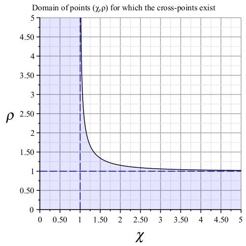
Figure VI.1: The plot of the critical value function $\rho_{\mathrm{cr}}\left(\chi\right)=\frac{\chi}{\sqrt{\chi^{2}-1}}$ for $\chi>1$. The shaded area represent all points $\left(\chi,\rho\right)$ for which there are exactly 4 cross-points. The blue dashed lines represent the asymptotes of $\rho_{\mathrm{cr}}\left(\chi\right)$ as $\chi\rightarrow 1$ and $\chi\rightarrow\infty$.

In other words, a cross-point is a point $\left(k,\omega\right)$ at which the dispersion relations for the GTL and the e-beam hold simultaneously. The solutions to the system of equations (VI.6) can be readily found as follows. We solve first equation $G_{\mathrm{B}}\left(k,\omega\right)=0$ yielding two solutions $\omega=k\pm 1$. Then we substitute for $\omega$ in the equation $G_{\mathrm{T}}\left(k,\omega\right)=0$ these two solutions obtaining two quadratic equations for $k$. Solving those quadratic equations for $k$ we find exactly four (counting the multiplicity) solutions (cross-points) to the system of equations (VI.6):

$$\left(\frac{\pm 1+d}{\chi^{2}-1},\frac{\pm 1+d}{\chi^{2}-1}\pm 1\right),\quad\left(\frac{\pm 1-d}{\chi^{2}-1},\frac{\pm 1-d}{\chi^{2}-1}\pm 1\right),$$ (VI.7)

$$d\stackrel{{\scriptstyle\mathrm{def}}}{{=}}d\left(\chi,\rho\right)=\sqrt{\rho^{2}+\left(1-\rho^{2}\right)\chi^{2}}=\sqrt{\rho^{2}\left(1-\chi^{2}\right)+\chi^{2}}.$$ (VI.8)

We note then either all four points defined by equations (VI.7) and (VI.8) have real components or they have complex-valued components depending on whether or not $d^{2}\left(\chi,\rho\right)\geq 0$. If $0<\chi\leq 1$ then it readily follows from equation (VI.8) that $d\geq 0$ and consequently all four solutions have real-valued components implying that we have exactly four (counting multiplicity) cross-points.

The cross-points are a commonly used in the TWT design since as one might expect the interaction between the GTL and the e-beam to be the strongest in a vicinity of these points.

If $\chi>1$ then the condition $d^{2}\left(\chi,\rho\right)\geq 0$ can be recast as

$$\rho\leq\rho_{\mathrm{cr}}\left(\chi\right)\stackrel{{\scriptstyle\mathrm{def}}}{{=}}\frac{\chi}{\sqrt{\chi^{2}-1}},\quad\chi>1.$$ (VI.9)

Evidently function $\rho_{\mathrm{cr}}\left(\chi\right)$ defined in relations (VI.9) determines the critical value $\rho_{\mathrm{cr}}\left(\chi\right)$ such that for $\chi>1$ the validity of inequality $\rho\leq\rho_{\mathrm{cr}}\left(\chi\right)$ determines if there are exactly four (counting multiplicity) cross-points or there are none. Since $\rho=\frac{\omega_{\mathrm{c}}}{\omega_{\mathrm{rp}}}$ we may view $\rho_{\mathrm{cr}}\left(\chi\right)$ can be viewed as critical vale of the relative low frequency cutoff $\rho=\frac{\omega_{\mathrm{c}}}{\omega_{\mathrm{rp}}}$. In other words $\rho=\frac{\omega_{\mathrm{c}}}{\omega_{\mathrm{rp}}}$ has to be smaller than $\rho_{\mathrm{cr}}\left(\chi\right)$ for the cross-points to exist.

Fig. VI.1 shows the plot of the critical low frequency cutoff $\rho_{\mathrm{cr}}\left(\chi\right)$. The corresponding critical value $\omega_{\mathrm{ccr}}$ of the the low cutoff frequency $\omega_{\mathrm{c}}$ is

$$\omega_{\mathrm{ccr}}=\frac{\chi}{\sqrt{\chi^{2}-1}}\omega_{\mathrm{rp}},$$ (VI.10)

and $\omega_{\mathrm{c}}$ must be smaller than $\omega_{\mathrm{ccr}}$ for the cross-points to exist. Note also the straight line defined by equation

$$\omega=k+\frac{\rho\sqrt{\chi^{2}-1}}{\chi},\quad\chi>1,$$ (VI.11)

is tangent to the GTL dispersion curve at the following point $\left(k,\omega\right):$

$$\left(k,\omega\right)=\left(\frac{\rho}{\chi\sqrt{\chi^{2}-1}},\frac{\rho\chi}{\sqrt{\chi^{2}-1}}\right),\quad\chi>1.$$ (VI.12)

VI.3 Dispersion graphs

We start with representing geometrically the dispersion relations (V.8) and (V.9) for the TWT, the GTL and the e-beam as follows:

$$\mathrm{Gr}_{\mathrm{TB}}\left(\gamma\right)\stackrel{{\scriptstyle\mathrm{def}}}{{=}}\left\{\left(k,\omega\right):\left[\omega^{2}-\left(\chi^{2}k^{2}+\rho^{2}\right)\right]\left[\left(k-\omega\right)^{2}-1\right]=\gamma k^{2}\left(\omega^{2}-\rho^{2}\right)\right\},\quad\gamma>0,$$ (VI.13)

$$\mathrm{Gr}_{\mathrm{T}}\stackrel{{\scriptstyle\mathrm{def}}}{{=}}\left\{\left(k,\omega\right):G_{\mathrm{T}}\left(k,\omega\right)=\omega^{2}-\left(\chi^{2}k^{2}+\rho^{2}\right)=0\right\},$$ (VI.14)

$$\mathrm{Gr}_{\mathrm{B}}\stackrel{{\scriptstyle\mathrm{def}}}{{=}}\left\{\left(k,\omega\right):G_{\mathrm{T}}\left(k,\omega\right)=\left(k-\omega\right)^{2}-1=0\right\},$$ (VI.15)

$$\mathrm{Gr}_{\mathrm{cT}}\stackrel{{\scriptstyle\mathrm{def}}}{{=}}\left\{\left(k,\omega\right):G_{\mathrm{cT}}\left(k,\omega\right)=k^{2}\left(\omega^{2}-\rho^{2}\right)=0\right\}.$$ (VI.16)

$$\mathrm{Gr}_{\mathrm{TB}}\left(0\right)\stackrel{{\scriptstyle\mathrm{def}}}{{=}}\mathrm{Gr}_{\mathrm{T}}\bigcup\mathrm{Gr}_{\mathrm{B}},$$ (VI.17)

$$\mathrm{Gr}_{\mathrm{TB}}\left(\infty\right)\stackrel{{\scriptstyle\mathrm{def}}}{{=}}\left\{\left(0,\omega\right):\left|\omega\right|\geq 1\right\}\bigcup\left\{\left(k,\rho\right),\left(k,-\rho\right):k\in\mathbb{R}\right\}.$$ (VI.18)

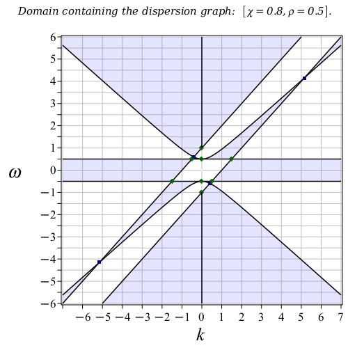
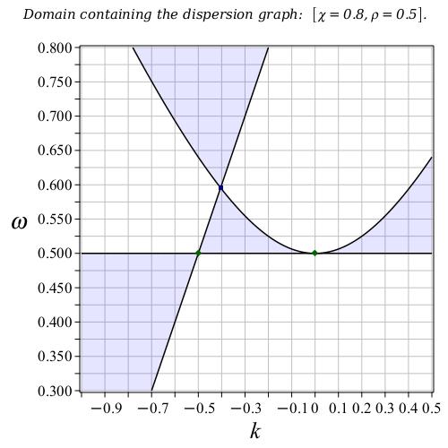
(a)                                                                             (b)

Figure VI.2: Dispersion domain $\mathbb{D}_{\mathrm{TB}}$ (where $R_{\mathrm{TB}}\left(k,\omega\right)>0$) is shown as shadowed (blue) area for $\chi=0.8$ and $\rho=0.5<1$: (a) complete plot in the designated window; (b) a zoomed fragment of the plot (a). Solid (black) curves represent the boundary $\partial\mathbb{D}_{\mathrm{TB}}$ of dispersion domain $\mathbb{D}_{\mathrm{TB}}$, that is the union $\mathrm{Gr}_{\mathrm{T}}\bigcup\mathrm{Gr}_{\mathrm{B}}\bigcup\mathrm{Gr}_{\mathrm{cT}}$ of graphs defined by equations (VI.14), (VI.15) and (VI.16). Diamond (green) dots represent focal points defined by equations (VI.1), square (blue) dots represent the cross-points $\mathrm{Gr}_{\mathrm{T}}\bigcap\mathrm{Gr}_{\mathrm{B}}$. For the chosen values of parameters the dispersion domain $\mathbb{D}_{\mathrm{TB}}$ has four unbounded connected components and four bounded ones for $\left|\omega\right|>\left|\rho\right|$.

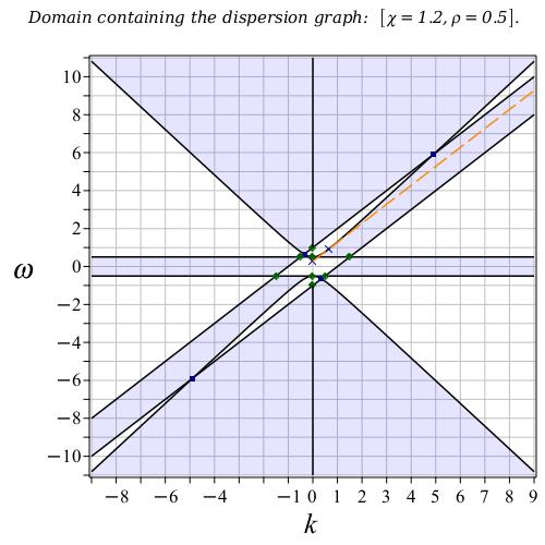
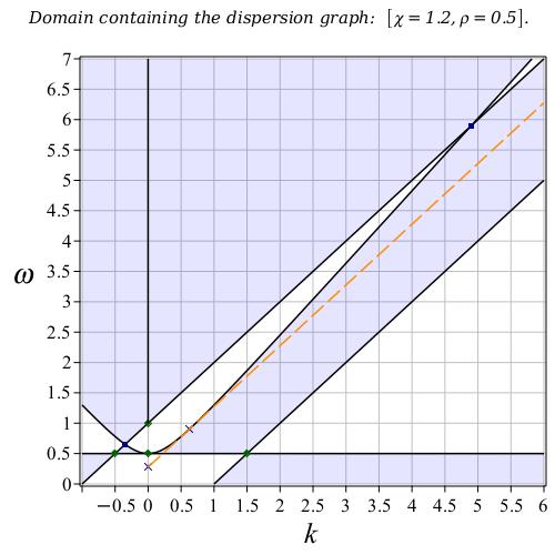
(a)                                                                     (b)

Figure VI.3: Dispersion domain $\mathbb{D}_{\mathrm{TB}}$ (where $R_{\mathrm{TB}}\left(k,\omega\right)>0$) is shown as shadowed (blue) area for $\chi=1.2$ and $\rho=0.5<1$: (a) complete plot in the designated window; (b) a zoomed fragment of the plot (a). Solid (black) curves represent the boundary $\partial\mathbb{D}_{\mathrm{TB}}$ of dispersion domain $\mathbb{D}_{\mathrm{TB}}$, that is the union $\mathrm{Gr}_{\mathrm{T}}\bigcup\mathrm{Gr}_{\mathrm{B}}\bigcup\mathrm{Gr}_{\mathrm{cT}}$ of graphs defined by equations (VI.14), (VI.15) and (VI.16). Diamond (green) dots represent focal points defined by equations (VI.1), square (blue) dots represent the cross-points $\mathrm{Gr}_{\mathrm{T}}\bigcap\mathrm{Gr}_{\mathrm{B}}$. The orange dashed straight line described by equation (VI.11) is parallel to the e-beam lines $\omega=k\pm 1$ and it is tangent to the graph $\mathrm{Gr}_{\mathrm{T}}$. The corresponding diagonal cross dot represents its intersection with $\omega$-axis described by (VI.12). For the chosen values of parameters the dispersion domain $\mathbb{D}_{\mathrm{TB}}$ has four unbounded connected components and no bounded ones for $\left|\omega\right|>\left|\rho\right|$.

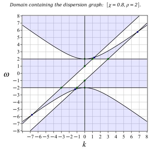
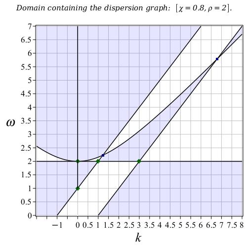
(a)                                                                         (b)

Figure VI.4: Dispersion domain $\mathbb{D}_{\mathrm{TB}}$ (where $R_{\mathrm{TB}}\left(k,\omega\right)>0$) is shown as shadowed (blue) area for $\chi=0.8$ and $\rho=2>1$: (a) complete plot in the designated window; (b) a zoomed fragment of the plot (a). Solid (black) curves represent the boundary $\partial\mathbb{D}_{\mathrm{TB}}$ of dispersion domain $\mathbb{D}_{\mathrm{TB}}$, that is the union $\mathrm{Gr}_{\mathrm{T}}\bigcup\mathrm{Gr}_{\mathrm{B}}\bigcup\mathrm{Gr}_{\mathrm{cT}}$ of graphs defined by equations (VI.14), (VI.15) and (VI.16). Diamond (green) dots represent focal points defined by equations (VI.1), square (blue) dots represent the cross-points $\mathrm{Gr}_{\mathrm{T}}\bigcap\mathrm{Gr}_{\mathrm{B}}$. For the chosen values of parameters the dispersion domain $\mathbb{D}_{\mathrm{TB}}$ has four unbounded connected components and two bounded ones for $\left|\omega\right|>\left|\rho\right|$.

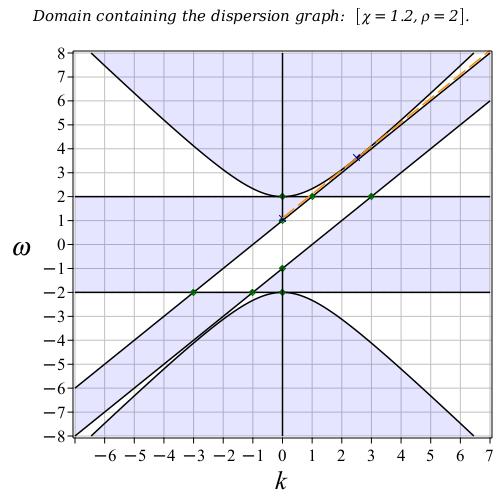
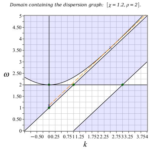
(a)                                                                     (b)

Figure VI.5: Dispersion domain $\mathbb{D}_{\mathrm{TB}}$ (where $R_{\mathrm{TB}}\left(k,\omega\right)>0$) is shown as shadowed (blue) area for $\chi=1.2$ and $\rho=2>1$: (a) complete plot in the designated window; (b) a zoomed fragment of the plot (a). Solid (black) curves represent the boundary $\partial\mathbb{D}_{\mathrm{TB}}$ of dispersion domain $\mathbb{D}_{\mathrm{TB}}$, that is the union $\mathrm{Gr}_{\mathrm{T}}\bigcup\mathrm{Gr}_{\mathrm{B}}\bigcup\mathrm{Gr}_{\mathrm{cT}}$ of graphs defined by equations (VI.14), (VI.15) and (VI.16). Diamond (green) dots represent focal points defined by equations (VI.1), square (blue) dots represent the cross-points $\mathrm{Gr}_{\mathrm{T}}\bigcap\mathrm{Gr}_{\mathrm{B}}$. The orange dashed straight line described by equation (VI.11) is parallel to the e-beam lines $\omega=k\pm 1$ and it is tangent to the graph $\mathrm{Gr}_{\mathrm{T}}$. The corresponding diagonal cross dot represents its intersection with $\omega$-axis described by (VI.12). For the chosen values of parameters the dispersion domain $\mathbb{D}_{\mathrm{TB}}$ has four unbounded connected components and no bounded ones for $\left|\omega\right|>\left|\rho\right|$.

Domain definitions (VI.16) and (VI.18) readily imply that

$$\mathrm{Gr}_{\mathrm{TB}}\left(\infty\right)\subseteq\mathrm{Gr}_{\mathrm{cT}}.$$ (VI.19)

It is instructive to see what happens with the graphs $\mathrm{Gr}_{\mathrm{TB}}\left(\gamma\right)$ as $\gamma\rightarrow 0$ and $\gamma\rightarrow+\infty$. The analysis of the plots of the graphs suggests that for any square $\mathrm{Sq}\left(a\right)=\left[-a,a\right]\times\left[-a,a\right]$, in $k\omega$-plane we have

$$\lim_{\gamma\rightarrow+0}\mathrm{Gr}_{\mathrm{TB}}\left(\gamma\right)\bigcap\mathrm{Sq}\left(a\right)=\left[\mathrm{Gr}_{\mathrm{T}}\bigcup\mathrm{Gr}_{\mathrm{B}}\right]\bigcap\mathrm{Sq}\left(a\right),\quad a>0,$$ (VI.20)

$$\lim_{\gamma\rightarrow+\infty}\mathrm{Gr}_{\mathrm{TB}}\left(\gamma\right)\bigcap\mathrm{Sq}\left(a\right)=\mathrm{Gr}_{\mathrm{TB}}\left(\infty\right)\bigcap\mathrm{Sq}\left(a\right),\quad a>0,$$ (VI.21)

that is points of the graph $\mathrm{Gr}_{\mathrm{TB}}\left(\gamma\right)$ residing also in square $\mathrm{Sq}\left(a\right)$ approach the union of graphs $\mathrm{Gr}_{\mathrm{T}}\bigcup\mathrm{Gr}_{\mathrm{B}}$ as $\gamma\rightarrow+0$ and these points approach graph $\mathrm{Gr}_{\mathrm{TB}}\left(\infty\right)$ as $\gamma\rightarrow+\infty$. Indeed, since $\left|k\right|,\left|\omega\right|\leq a$ equations (V.4) and (V.8) imply limit relations (VI.20) and (VI.21).

Let us introduce the following parallelogram domain

$$\Pi_{\mathrm{TB}}=\left\{\left(k,\omega\right):k-1<\omega<k+1,\quad-\rho<\omega<\rho\right\}.$$ (VI.22)

Note that based on an elementary analysis of the signs of the factors $G_{\mathrm{T}}\left(k,\omega\right)$, $G_{\mathrm{B}}\left(k,\omega\right)$ and $G_{\mathrm{cT}}\left(k,\omega\right)$ and the definition (V.9), (V.10) of function $R_{\mathrm{TB}}\left(k,\omega\right)$ we can obtain the following inequality

$$R_{\mathrm{TB}}\left(k,\omega\right)<0,\quad\left(k,\omega\right)\in\Pi_{\mathrm{TB}}.$$ (VI.23)

Consequently, there no real-valued solutions to the dispersion equation $R_{\mathrm{TB}}\left(k,\omega\right)=\gamma>0$ in parallelogram $\Pi_{\mathrm{TB}}$, that is

$$\mathrm{Gr}_{\mathrm{TB}}\left(\gamma\right)\bigcap\Pi_{\mathrm{TB}}=\emptyset.$$ (VI.24)

Note also that for $k=0$ the dispersion equation (V.4) turns into

$$\left[\omega^{2}-\rho^{2}\right]\left[\omega^{2}-1\right]=0,$$ (VI.25)

readily implying that it has no real-valued solutions for $\omega\neq\pm 1$ with an exception of $\omega=\pm\rho$ in case when $\rho\neq 1$.

VI.4 Dispersion domains

In this section we identify domains that contain the TWT dispersion graphs $\mathrm{Gr}_{\mathrm{TB}}\left(\gamma\right)$ defined by equations (VI.13) based on the signs of the factors $G_{\mathrm{T}}\left(k,\omega\right)$, $G_{\mathrm{B}}\left(k,\omega\right)$ and $G_{\mathrm{cT}}\left(k,\omega\right)$ entering the TWT dispersion relation (V.4), (V.4) , (V.9) and (V.10). We proceed with introducing dispersion domains $\mathbb{D}_{\mathrm{TB}}$, $\mathbb{D}_{\mathrm{T}}\left(\sigma\right)$ and $\mathbb{D}_{\mathrm{B}}\left(\sigma\right)$ for $\sigma=\pm 1$ related respectively to the TWT, the GTL and the e-beam as follows:

$$\mathbb{D}_{\mathrm{TB}}\stackrel{{\scriptstyle\mathrm{def}}}{{=}}\left\{\left(k,\omega\right)\in\mathbb{R}^{2}:R_{\mathrm{TB}}\left(k,\omega\right)>0\right\}=\bigcup_{\gamma>0}\mathrm{Gr}_{\mathrm{TB}}\left(\gamma\right),$$ (VI.26)

$$\mathbb{D}_{\mathrm{T}}\left(\sigma\right)\stackrel{{\scriptstyle\mathrm{def}}}{{=}}\left\{\left(k,\omega\right):\mathrm{sign}\left[G_{\mathrm{T}}\left(k,\omega\right)\right]=\mathrm{sign}\left[\omega^{2}-\left(\chi^{2}k^{2}+\rho^{2}\right)\right]=\sigma\right\},\quad\sigma=\pm 1,$$ (VI.27)

$$\mathbb{D}_{\mathrm{B}}\left(\sigma\right)\stackrel{{\scriptstyle\mathrm{def}}}{{=}}\left\{\left(k,\omega\right):\mathrm{sign}\left[G_{\mathrm{B}}\left(k,\omega\right)\right]=\mathrm{sign}\left[\left(k-\omega\right)^{2}-1\right]=\sigma\right\},\quad\sigma=\pm 1.$$ (VI.28)

In addition to that, we make use of domain

$$\mathbb{D}_{\mathrm{cT}}\left(\sigma\right)\stackrel{{\scriptstyle\mathrm{def}}}{{=}}\left\{\left(k,\omega\right):\mathrm{sign}\left[G_{\mathrm{cT}}\left(k,\omega\right)\right]=\mathrm{sign}\left[\omega^{2}-\rho^{2}\right]=\sigma\right\},\quad\sigma=\pm 1.$$ (VI.29)

Based on definitions (VI.14), (VI.15) and (VI.16) we obtain

$$\partial\mathbb{D}_{\mathrm{TB}}=\mathrm{Gr}_{\mathrm{T}}\bigcup\mathrm{Gr}_{\mathrm{B}}\bigcup\mathrm{Gr}_{\mathrm{cT}}.$$ (VI.30)

VII Dispersion curves for varying coupling

We exhibit and discuss here a series of plots of the TWT dispersion curves generated for different values of the TWT principle parameter $\gamma$, see Figures II.1, II.2 and Figures VII.1-VII.9. The goal we pursue when generating these plots is to demonstrate different topological patterns occurring for different sets of the involved parameters. In particular, the plots show qualitatively different topological patterns that occur when: (i) $\rho>1$ or $\rho<1$; (ii) $\chi>1$ or $\chi<1$; (iii) $\gamma$ is small or large. The point for generating a number of dispersive curves for particular selections of sets of different $\gamma$ is to demonstrate: (i) the closer proximity of the TWT dispersion curves for smaller values $\gamma$ to the dispersion curves of the non-interacting GTL and the e-beam used as the reference frames; (ii) the focal points that belong to all the TWT dispersion curves. Another benefit of looking into the TWT dispersive curves for small values of $\gamma$ is that indicate their naturally hybrid nature. Indeed, when the principle TWT parameter $\gamma$, which also plays the role of a coupling constant in the TWT dispersion equations (V.3), gets smaller some parts each of the TWT dispersive curves get closer to the dispersion curves of the non-interacting GTL whereas other parts get closer to the dispersion curves of the non-interacting e-beam. To see the hybrid natures of the TWT dispersive curves we integrated into each plot the dispersion curves of non-interacting GTL and the e-beam as reference frames.

We invite a curious reader to explore Figures II.1, II.2 and Figures VII.1-VII.9 displaying different patterns of the selected sets of the TWT dispersion curves including focal points and the dispersion curves of the non-interacting GTL and the e-beam used as the reference frames.

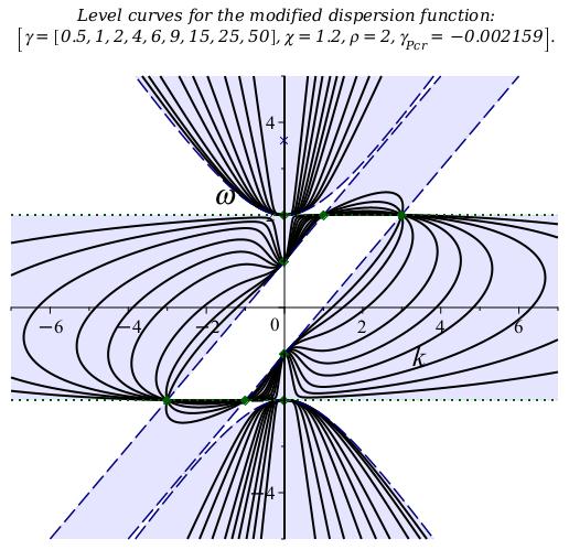
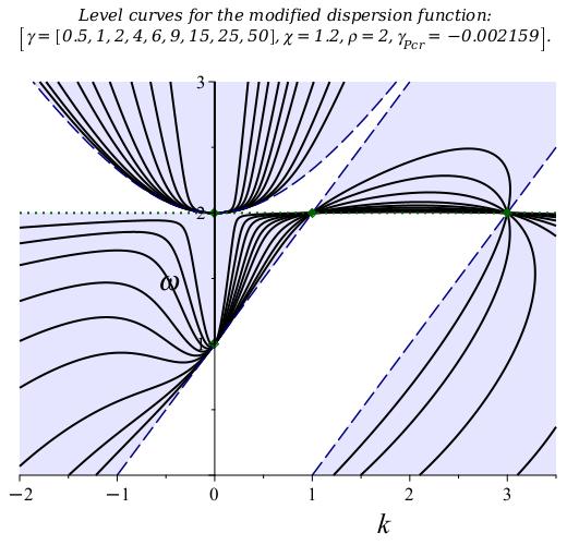
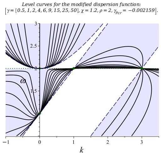
(a)                                               (b)                                               (c)

Figure VII.1: Dispersion curves of the TWT dispersion relations (V.3) and (V.4) for $\chi=1.2$, $\rho=0.5<1$ and $\gamma=0.5,1,2,4,6,9,15,25,50$, $\gamma_{\mathrm{Pcr}}\cong 0.002641$: (a) complete plot in the designated window; (b) a zoomed fragment of (a); (c) a zoomed fragment of (b). Solid (black) curves represent the TWT dispersion curves for indicated values of $\gamma$; dashed (blue) curves represent the dispersion curves of non-interacting TL and the e-beam for $\gamma=0$ as a reference. Shaded area identifies the dispersion domain $\mathbb{D}_{\mathrm{TB}}$, that is where $R_{\mathrm{TB}}\left(k,\omega\right)>0$. Doted (green) horizontal straight lines represents points $\left(k,\pm\rho\right)$. Note the dispersion curves $\mathrm{Gr}_{\mathrm{TB}}\left(\gamma\right)$ pass through focal points defined by equations (VI.1) marked as circle (green) dots. Square (blue) dots mark the TWT cross-points (see equations (VI.7), (VI.8)). Note also that the smaller $\gamma$ gets the closer graph $\mathrm{Gr}_{\mathrm{TB}}\left(\gamma\right)$ gets to $\mathrm{Gr}_{\mathrm{TB}}\left(0\right)=\mathrm{Gr}_{\mathrm{T}}\bigcup\mathrm{Gr}_{\mathrm{B}}$, whereas the larger $\gamma$ gets the closer graph $\mathrm{Gr}_{\mathrm{TB}}\left(\gamma\right)$ gets to $\mathrm{Gr}_{\mathrm{TB}}\left(\infty\right)$ defined by equation (VI.18).

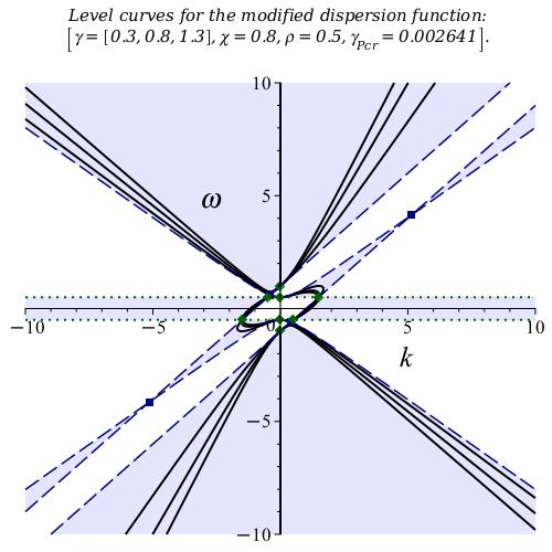
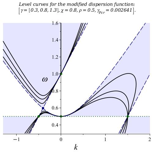
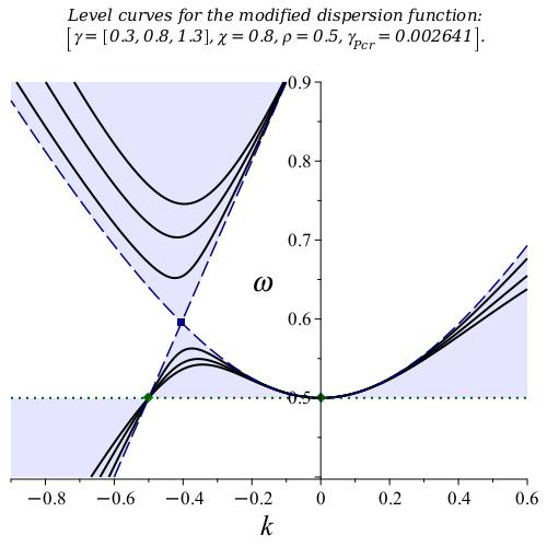
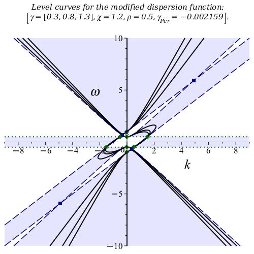
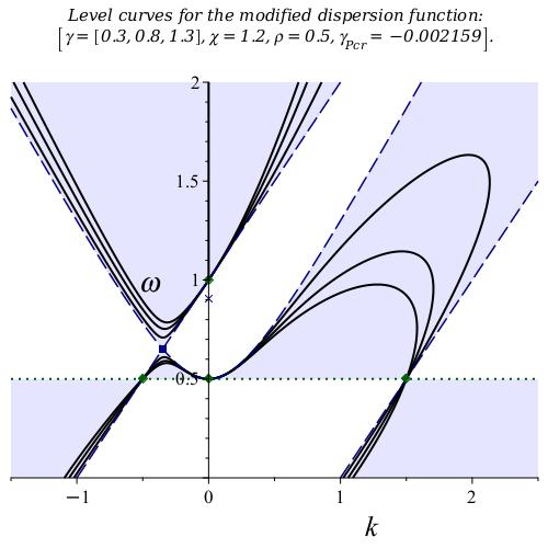
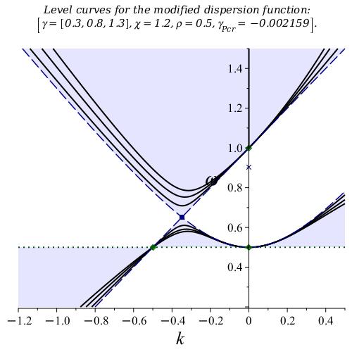
(a)                                               (b)                                               (c)

Figure VII.2: Dispersion curves of the TWT dispersion relations (V.3) and (V.4) for $\chi=0.8$, $\rho=0.5<1$ and $\gamma=0.3,0.8,1.3$, $\gamma_{\mathrm{Pcr}}\cong 0.002641$: (a) complete plot in the designated window; (b) a zoomed fragment of (a); (c) a zoomed fragment of (b). Solid (black) curves represent the TWT dispersion curves for indicated values of $\gamma$; dashed (blue) curves represent the dispersion curves of non-interacting TL and the e-beam for $\gamma=0$ as a reference. Shaded area identifies the dispersion domain $\mathbb{D}_{\mathrm{TB}}$, that is where $R_{\mathrm{TB}}\left(k,\omega\right)>0$. Doted (green) horizontal straight lines represents points $\left(k,\pm\rho\right)$. Note the dispersion curves pass through focal points $\left(0,\pm 1\right)$. Note the dispersion curves $\mathrm{Gr}_{\mathrm{TB}}\left(\gamma\right)$ pass through focal points defined by equations (VI.1) marked as circle (green) dots. Square (blue) dots mark the TWT cross-points (see equations (VI.7), (VI.8)). Note also that the smaller $\gamma$ gets the closer graph $\mathrm{Gr}_{\mathrm{TB}}\left(\gamma\right)$ gets to $\mathrm{Gr}_{\mathrm{TB}}\left(0\right)=\mathrm{Gr}_{\mathrm{T}}\bigcup\mathrm{Gr}_{\mathrm{B}}$, whereas the larger $\gamma$ gets the closer graph $\mathrm{Gr}_{\mathrm{TB}}\left(\gamma\right)$ gets to $\mathrm{Gr}_{\mathrm{TB}}\left(\infty\right)$ defined by equation (VI.18).

(a)                                               (b)                                               (c)

Figure VII.3: Dispersion curves of the TWT dispersion relations (V.3) and (V.4) for $\chi=1.2$, $\rho=0.5<1$ and $\gamma=0.3,0.8,1.3$, $\gamma_{\mathrm{Pcr}}\cong-0.002159$: (a) complete plot in the designated window; (b) a zoomed fragment of (a); (c) a zoomed fragment of (b). Solid (black) curves represent the TWT dispersion curves for indicated values of $\gamma$; dashed (blue) curves represent the dispersion curves of non-interacting TL and the e-beam for $\gamma=0$ as a reference. Shaded area identifies the dispersion domain $\mathbb{D}_{\mathrm{TB}}$, that is where $R_{\mathrm{TB}}\left(k,\omega\right)>0$. Doted (green) horizontal straight lines represents points $\left(k,\pm\rho\right)$. Note the dispersion curves pass through focal points $\left(0,\pm 1\right)$. Note the dispersion curves $\mathrm{Gr}_{\mathrm{TB}}\left(\gamma\right)$ pass through focal points defined by equations (VI.1) marked as circle (green) dots. Square (blue) dots mark the TWT cross-points (see equations (VI.7), (VI.8)). Note also that the smaller $\gamma$ gets the closer graph $\mathrm{Gr}_{\mathrm{TB}}\left(\gamma\right)$ gets to $\mathrm{Gr}_{\mathrm{TB}}\left(0\right)=\mathrm{Gr}_{\mathrm{T}}\bigcup\mathrm{Gr}_{\mathrm{B}}$, whereas the larger $\gamma$ gets the closer graph $\mathrm{Gr}_{\mathrm{TB}}\left(\gamma\right)$ gets to $\mathrm{Gr}_{\mathrm{TB}}\left(\infty\right)$ defined by equation (VI.18).

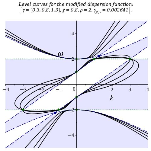
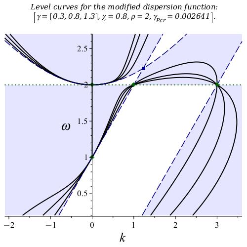
(a)                                                            (b)

Figure VII.4: Dispersion curves of the TWT dispersion relations (V.3) and (V.4) for $\chi=0.8$, $\rho=2>1$ and $\gamma=0.3,0.8,1.3$, $\gamma_{\mathrm{Pcr}}\cong 0.002641$: (a) complete plot in the designated window; (b) a zoomed fragment of (a); (c) a zoomed fragment of (b). Solid (black) curves represent the TWT dispersion curves for indicated values of $\gamma$; dashed (blue) curves represent the dispersion curves of non-interacting TL and the e-beam for $\gamma=0$ as a reference. dashed (blue) curves represent the dispersion curves of non-interacting TL and the e-beam. Shaded area identifies the dispersion domain $\mathbb{D}_{\mathrm{TB}}$, that is where $R_{\mathrm{TB}}\left(k,\omega\right)>0$. Doted (green) horizontal straight lines represents points $\left(k,\pm\rho\right)$. Note the dispersion curves passing through points focal points $\left(0,\pm 1\right)$. Note the dispersion curves $\mathrm{Gr}_{\mathrm{TB}}\left(\gamma\right)$ pass through focal points defined by equations (VI.1) marked as circle (green) dots. Square (blue) dots mark the TWT cross-points (see equations (VI.7), (VI.8)). Note also that the smaller $\gamma$ gets the closer graph $\mathrm{Gr}_{\mathrm{TB}}\left(\gamma\right)$ gets to $\mathrm{Gr}_{\mathrm{TB}}\left(0\right)=\mathrm{Gr}_{\mathrm{T}}\bigcup\mathrm{Gr}_{\mathrm{B}}$, whereas the larger $\gamma$ gets the closer graph $\mathrm{Gr}_{\mathrm{TB}}\left(\gamma\right)$ gets to $\mathrm{Gr}_{\mathrm{TB}}\left(\infty\right)$ defined by equation (VI.18).

Figures VII.5-VII.9 indicate in particular the low and the high frequency cutoff for the convection instability that are similar to what was found in SchaFig [29] for the special case $\rho=0$.

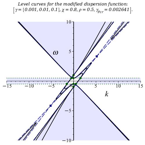
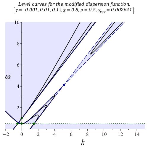
(a)                                                                     (b)

Figure VII.5: Dispersion curves of the TWT dispersion relations (V.3) and (V.4) for $\chi=0.8$, $\rho=0.5<1$ and $\gamma=0.001,0.01,0.1$, $\gamma_{\mathrm{Pcr}}\cong 0.002641$: (a) complete plot in the designated window; (b) a zoomed fragment of (a); (c) a zoomed fragment of (b). Solid (black) curves represent the TWT dispersion curves for indicated values of $\gamma$; dashed (blue) curves represent the dispersion curves of non-interacting TL and the e-beam for $\gamma=0$ as a reference. Shaded area identifies the dispersion domain $\mathbb{D}_{\mathrm{TB}}$, that is where $R_{\mathrm{TB}}\left(k,\omega\right)>0$. Doted (green) horizontal straight lines represents points $\left(k,\pm\rho\right)$. Note the dispersion curves $\mathrm{Gr}_{\mathrm{TB}}\left(\gamma\right)$ pass through focal points defined by equations (VI.1) marked as circle (green) dots. Square (blue) dots mark the TWT cross-points (see equations (VI.7), (VI.8)). Note also that the smaller $\gamma$ gets the closer graph $\mathrm{Gr}_{\mathrm{TB}}\left(\gamma\right)$ gets to $\mathrm{Gr}_{\mathrm{TB}}\left(0\right)=\mathrm{Gr}_{\mathrm{T}}\bigcup\mathrm{Gr}_{\mathrm{B}}$, whereas the larger $\gamma$ gets the closer graph $\mathrm{Gr}_{\mathrm{TB}}\left(\gamma\right)$ gets to $\mathrm{Gr}_{\mathrm{TB}}\left(\infty\right)$ defined by equation (VI.18).

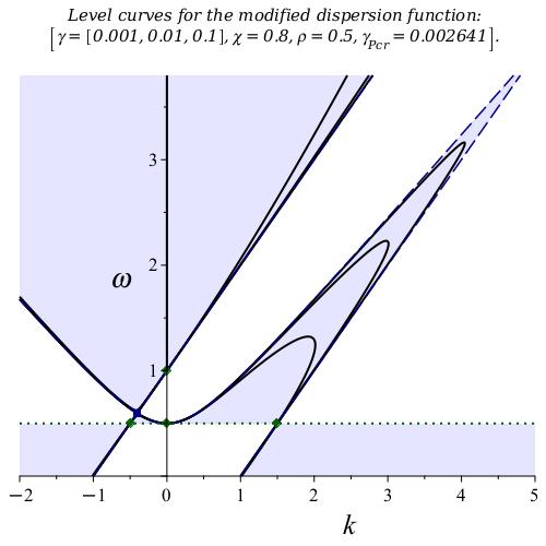
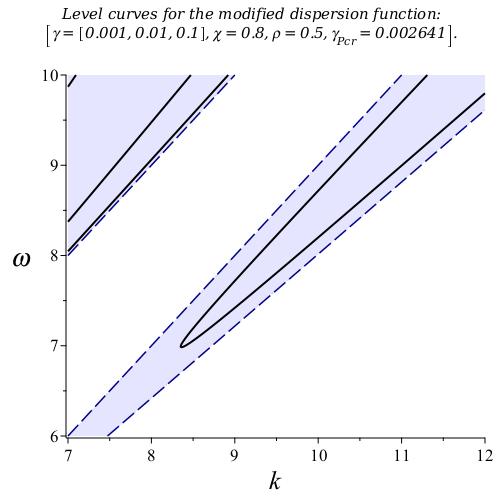
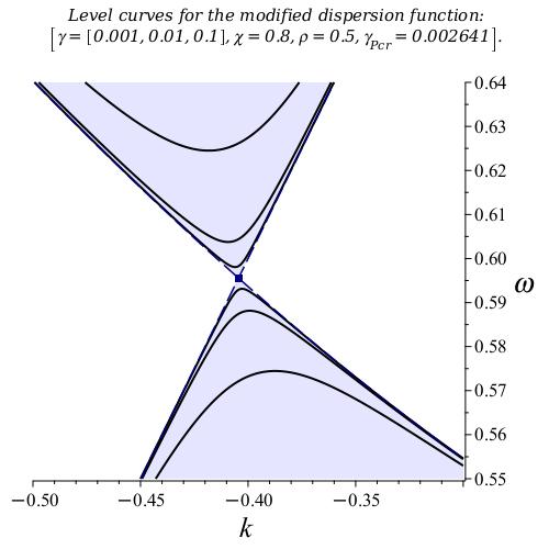
(a)                                               (b)                                               (c)

Figure VII.6: Dispersion curves of the TWT dispersion relations (V.3) and (V.4) for $\chi=0.8$, $\rho=0.5<1$ and $\gamma=0.001,0.01,0.1$, $\gamma_{\mathrm{Pcr}}\cong 0.002641$: (a) zoomed fragment of Fig. VII.5(b) for $k>0$; (b); another zoomed fragment of Fig. VII.5(b) for $k>0$; (c) zoomed fragment of Fig. VII.5(a) for $k<0$. Solid (black) curves represent the TWT dispersion curves for indicated values of $\gamma$; dashed (blue) curves represent the dispersion curves of non-interacting TL and the e-beam for $\gamma=0$ as a reference. Shaded area identifies the dispersion domain $\mathbb{D}_{\mathrm{TB}}$, that is where $R_{\mathrm{TB}}\left(k,\omega\right)>0$. Doted (blue) horizontal straight lines represents points $\left(k,\pm\rho\right)$. Doted (green) horizontal straight lines represents points $\left(k,\pm\rho\right)$. Note the dispersion curves $\mathrm{Gr}_{\mathrm{TB}}\left(\gamma\right)$ pass through focal points defined by equations (VI.1) marked as circle (green) dots. Square (blue) dots mark the TWT cross-points (see equations (VI.7), (VI.8)). Note also that the smaller $\gamma$ gets the closer graph $\mathrm{Gr}_{\mathrm{TB}}\left(\gamma\right)$ gets to $\mathrm{Gr}_{\mathrm{TB}}\left(0\right)=\mathrm{Gr}_{\mathrm{T}}\bigcup\mathrm{Gr}_{\mathrm{B}}$, whereas the larger $\gamma$ gets the closer graph $\mathrm{Gr}_{\mathrm{TB}}\left(\gamma\right)$ gets to $\mathrm{Gr}_{\mathrm{TB}}\left(\infty\right)$ defined by equation (VI.18).

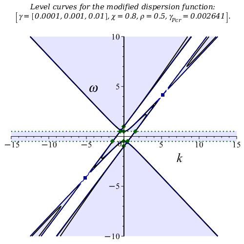
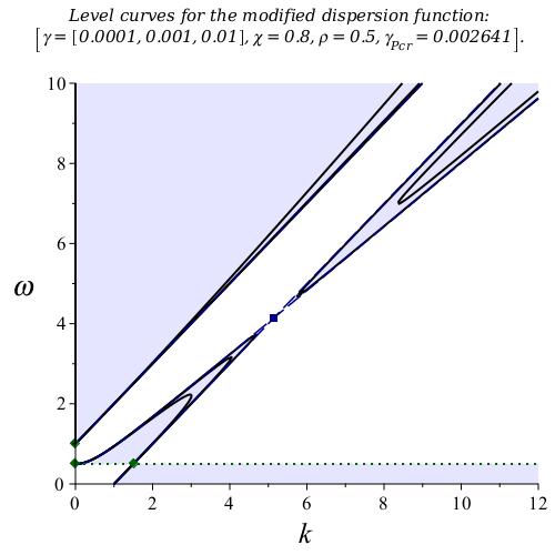
(a)                                                            (b)

Figure VII.7: Dispersion curves of the TWT dispersion relations (V.3) and (V.4) for $\chi=0.8$, $\rho=0.5<1$ and $\gamma=0.0001,0.001,0.01$, $\gamma_{\mathrm{Pcr}}\cong 0.002641$: (a) complete plot in the designated window; (b) a zoomed fragment of (a); (c) a zoomed fragment of (b). Solid (black) curves represent the TWT dispersion curves for indicated values of $\gamma$; dashed (blue) curves represent the dispersion curves of non-interacting TL and the e-beam for $\gamma=0$ as a reference. Shaded area identifies the dispersion domain $\mathbb{D}_{\mathrm{TB}}$, that is where $R_{\mathrm{TB}}\left(k,\omega\right)>0$. Doted (green) horizontal straight lines represents points $\left(k,\pm\rho\right)$. Note the dispersion curves $\mathrm{Gr}_{\mathrm{TB}}\left(\gamma\right)$ pass through focal points defined by equations (VI.1) marked as circle (green) dots. Square (blue) dots mark the TWT cross-points (see equations (VI.7), (VI.8)). Note also that the smaller $\gamma$ gets the closer graph $\mathrm{Gr}_{\mathrm{TB}}\left(\gamma\right)$ gets to $\mathrm{Gr}_{\mathrm{TB}}\left(0\right)=\mathrm{Gr}_{\mathrm{T}}\bigcup\mathrm{Gr}_{\mathrm{B}}$, whereas the larger $\gamma$ gets the closer graph $\mathrm{Gr}_{\mathrm{TB}}\left(\gamma\right)$ gets to $\mathrm{Gr}_{\mathrm{TB}}\left(\infty\right)$ defined by equation (VI.18).

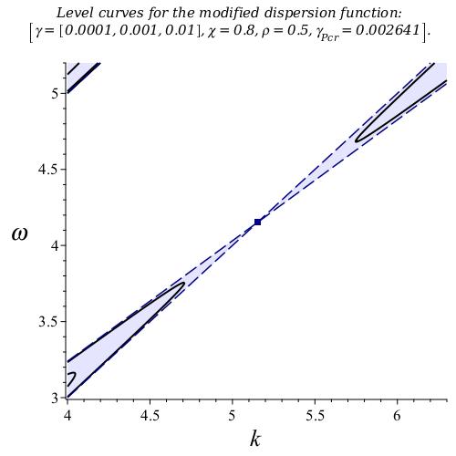
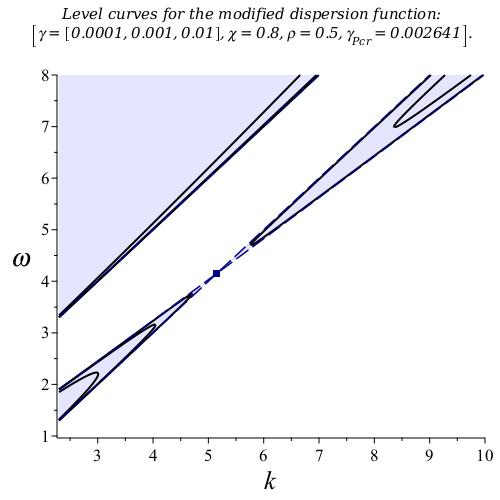
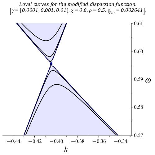
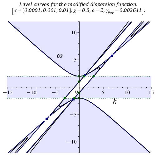
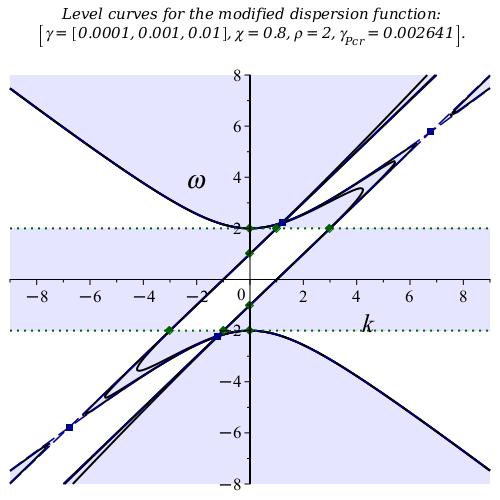
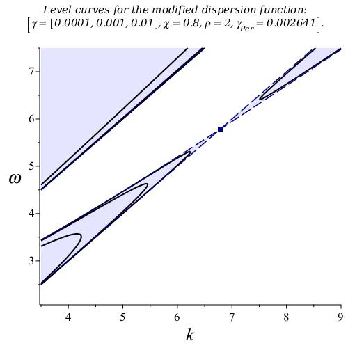
(a)                                           (b)                                           (c)

Figure VII.8: Dispersion curves of the TWT dispersion relations (V.3) and (V.4) for $\chi=0.8$, $\rho=0.5<1$ and $\gamma=0.0001,0.001,0.01$, $\gamma_{\mathrm{Pcr}}\cong 0.002641$: (a) zoomed fragment of Fig. VII.7(b) for $k>0$; (b) another zoomed fragment of Fig. VII.7(b) for $k>0$; (c) zoomed fragment of Fig. VII.7(a) for $k<0$. Solid (black) curves represent the TWT dispersion curves for indicated values of $\gamma$; dashed (blue) curves represent the dispersion curves of non-interacting TL and the e-beam for $\gamma=0$ as a reference. Shaded area identifies the dispersion domain $\mathbb{D}_{\mathrm{TB}}$, that is where $R_{\mathrm{TB}}\left(k,\omega\right)>0$. Doted (green) horizontal straight lines represents points $\left(k,\pm\rho\right)$. Note the dispersion curves $\mathrm{Gr}_{\mathrm{TB}}\left(\gamma\right)$ pass through focal points defined by equations (VI.1) marked as circle (green) dots. Square (blue) dots mark the TWT cross-points (see equations (VI.7), (VI.8)). Note also that the smaller $\gamma$ gets the closer graph $\mathrm{Gr}_{\mathrm{TB}}\left(\gamma\right)$ gets to $\mathrm{Gr}_{\mathrm{TB}}\left(0\right)=\mathrm{Gr}_{\mathrm{T}}\bigcup\mathrm{Gr}_{\mathrm{B}}$, whereas the larger $\gamma$ gets the closer graph $\mathrm{Gr}_{\mathrm{TB}}\left(\gamma\right)$ gets to $\mathrm{Gr}_{\mathrm{TB}}\left(\infty\right)$ defined by equation (VI.18).

(a)                                               (b)                                               (c)

Figure VII.9: Dispersion curves of the TWT dispersion relations (V.3) and (V.4) for $\chi=0.8$, $\rho=2>1$ and $\gamma=0.0001,0.001,0.01$, $\gamma_{\mathrm{Pcr}}\cong 0.002641$: (a) zoomed fragment of Fig. VII.7(b) for $k>0$; (b); another zoomed fragment of Fig. VII.7(b) for $k>0$; (c) zoomed fragment of Fig. VII.7(a) for $k<0$. Solid (black) curves represent the TWT dispersion curves for indicated values of $\gamma$; dashed (blue) curves represent the dispersion curves of non-interacting TL and the e-beam for $\gamma=0$ as a reference. Shaded area identifies the dispersion domain $\mathbb{D}_{\mathrm{TB}}$, that is where $R_{\mathrm{TB}}\left(k,\omega\right)>0$. Doted (green) horizontal straight lines represents points $\left(k,\pm\rho\right)$. Note the dispersion curves $\mathrm{Gr}_{\mathrm{TB}}\left(\gamma\right)$ pass through focal points defined by equations (VI.1) marked as circle (green) dots. Square (blue) dots mark the TWT cross-points (see equations (VI.7), (VI.8)). Note also that the smaller $\gamma$ gets the closer graph $\mathrm{Gr}_{\mathrm{TB}}\left(\gamma\right)$ gets to $\mathrm{Gr}_{\mathrm{TB}}\left(0\right)=\mathrm{Gr}_{\mathrm{T}}\bigcup\mathrm{Gr}_{\mathrm{B}}$, whereas the larger $\gamma$ gets the closer graph $\mathrm{Gr}_{\mathrm{TB}}\left(\gamma\right)$ gets to $\mathrm{Gr}_{\mathrm{TB}}\left(\infty\right)$ defined by equation (VI.18).

VIII Instabilities and dispersion-instability graphs

It is clear that the electron beam has to supply the exponentially growing in space - the phenomenon known as convection instability. Slowing down of the EM wave facilitates more efficient interaction with the electron flow manifested in electron bunching and synchronism that are essential for the RF signal amplification. The flow of electrons in TWT move with nearly constant velocity and loose some of their kinetic energy to the EM wave. This kind of energy transfer is observed in the Cherenkov radiation phenomenon that can be viewed then as a physical foundation for the convection instability and consequent RF signal amplification, [5, Sec. 1.1-1.2, 4.4, 4.8-4.9, 7.3, 7.6; Chap. 8]. Based on a Lagrangian field theory, we developed in our work SchaFig [29] a convincing argument that the collective Cherenkov effect in TWTs is, in fact, a convective instability, that is, amplification. We also derive there expressions of the low- and high-frequency cutoffs for amplification in TWTs. Relations “wave-particle interactions” and origins of instability is discussed in FigTWTbk [11, Chap. 5].

As to instabilities in general we remind the reader that as amplification regimes are based on the convective instability oscillation regimes are based on the absolute instability, [31], [4]. The difference between the two instabilities in a nutshell is as follows. The convective instability is when the original pulse disturbance convect from its origin in space as it grows in amplitude but at every fixed point of space the disturbance is bounded by a time independent constant. In contrast, the absolute instability is when the original pulse disturbance grows without a bound in time at least in some points of space. Note that the labeling of an instability is always with respect to a particular reference frame, since a convective instability would appear as an absolute instability to an observer moving along with the ”pulse”.

In order to identify convection and absolutes instabilities in TWTs one commonly considers the relevant eigenmodes of the following exponential form

$$f_{\omega,k}\left(z,t\right)=a_{\omega k}\exp\left\{-\mathrm{i}\left(\omega t-kz\right)\right\},$$ (VIII.1)

where $a_{\omega k}$ is a complex-valued constant and $\omega$ and $k$ are respectively the frequency and wave-number that can possibly be complex-valued. Importantly, for $f_{\omega,k}\left(z,t\right)$ to be an eigenmode $\omega$ and $k$, that can be complex-valued now, must satisfy the TWT dispersion relations (IV.2), (IV.4), (V.3) and (V.4). In the case when $\omega$ is real and $\Im\left(k\right)\neq 0$ function $\left|f_{\omega k}\left(z,t\right)\right|$ grows or decays exponentially if $z\rightarrow\pm\infty$ and we refer to this situation as convection instability associated with amplification regimes. In the case $k$ is real but $\Im\left(\omega\right)\neq 0$ function $\left|f_{\omega k}\left(z,t\right)\right|$ grows or decays exponentially if $t\rightarrow\pm\infty$ and we refer to this situation as absolute instability associated with (exponentially growing) oscillations regimes.

Note that for complex-valued $\omega$ and $k$ the phase velocity $u=\frac{\omega}{\omega}$ can be also complex-valued satisfying the TWT velocity dispersion relations (IV.3), (IV.12).

In Sections VI and VII we considered the graphs of the conventional dispersion relations. It is useful to integrate the information about the TWT instabilities into the dispersion relations using the concept of dispersion-instability graph that we have developed in FigTWTbk [11, Chap. 7]. Typical examples of the dispersion-instability graphs are shown in Figures II.3-VIII.5. Recall that the conventional dispersion relations are defined as the relations between real-valued frequency $\omega$ and real-valued wavenumber $k$ associated with the relevant eigenmodes. In the case of the convection instability frequency $\omega$ is real and wavenumber $k$ can be complex-valued, whereas in the case of absolute instability $k$ is real and $\omega$ can be complex-valued. To represent the corresponding modes geometrically as points in real $k\omega$-plane we proceed as follows, [11, 7].

In this paper we focus primarily on the convection instability with the only exception made in Section X where we consider also absolutely unstable modes.

First, let us consider the case of the convection instability when $\omega$ is real and $k$ is complex-valued. In this case we parametrize every mode of the TWT system uniquely by the pair $\left(k\left(\omega\right),\omega\right)$ where $\omega$ is its frequency and $k\left(\omega\right)$ is its wavenumber. If $k\left(\omega\right)$ is degenerate, it is counted a number of times according to its multiplicity. We can naturally partition all the system modes represented by pairs $\left(k\left(\omega\right),\omega\right)$ into two distinct classes – oscillatory modes and (convectively) unstable ones – based on whether the wavenumber $k\left(\omega\right)$ is real- or complex-valued with $\Im\left\{k\left(\omega\right)\right\}\neq 0$. We refer to a mode (eigenmode) of the system as an oscillatory mode if its wavenumber $k\left(\omega\right)$ is real-valued. We associate with such an oscillatory mode point $\left(k\left(\omega\right),\omega\right)$ in the $k\omega$-plane with $k$ being the horizontal axis and $\omega$ being the vertical one. Similarly, we refer to a mode (eigenmode) of the system as a convectively unstable mode if its wavenumber $k=k\left(\omega\right)$ is complex-valued with a nonzero imaginary part, that is, $\Im\left\{k\left(\omega\right)\right\}\neq 0$. We associate with such an unstable mode point $\left(\Re\left\{k\left(\omega\right)\right\},\omega\right)$ in the $k\omega$-plane.

Based on the above considerations, we represent the set of all the oscillatory and convectively unstable modes of the system geometrically by the set of the corresponding modal points $\left(k\left(\omega\right),\omega\right)$ and $\left(\Re\left\{k\left(\omega\right)\right\},\omega\right)$ in the $k\omega$-plane. We name this set the dispersion-instability graph. To distinguish graphically points $\left(k\left(\omega\right),\omega\right)$ associated with oscillatory modes when $k\left(\omega\right)$ is real-valued from points $\left(\Re\left\{k\left(\omega\right)\right\},\omega\right)$ associated with unstable modes when $k\left(\omega\right)$ is complex-valued with $\Im\left\{k\left(\omega\right)\right\}\neq 0$ we show points $\Im\left\{k\left(\omega\right)\right\}=0$ in black color whereas points with $\Im\left\{k\left(\omega\right)\right\}\neq 0$ are shown in red color. The corresponding curves are shown respectively as the solid (black) and solid (red) curves. We remind that every point $\left(\Re\left\{k\left(\omega\right)\right\},\omega\right)$ with $\Im\left\{k\left(\omega\right)\right\}\neq 0$ represents exactly two complex conjugate convectively unstable modes associated with $\pm\Im\left\{k\left(\omega\right)\right\}$.

To integrate into the dispersion-instability graph the information about the absolute instability, we proceed similarly to the case of the convection instability. In this case we assume $k$ to be real whereas $\omega$ can be complex-valued. Then every relevant mode can be represented uniquely by the pair $\left(k,\omega\left(k\right)\right)$ where $\omega\left(k\right)$ is the mode frequency and $k$ is its wavenumber. If $\omega\left(k\right)$ is degenerate, it is counted a number of times according to its multiplicity. Similarly to the convection instability we partition all the modes into two distinct classes – oscillatory modes and unstable ones – based on whether the frequency $\omega\left(k\right)$ is real- or complex-valued with $\Im\left\{\omega\left(k\right)\right\}\neq 0$. As before we refer to a mode (eigenmode) of the system as an oscillatory mode if its frequency is real-valued. Note that the class of oscillatory modes for both convection and absolute instability are exactly the same. We refer to a mode (eigenmode) of the system as absolutely unstable mode if its frequency $\omega\left(k\right)$ is complex-valued with a nonzero imaginary part, that is, $\Im\left\{\omega\left(k\right)\right\}\neq 0$. We associate with such an absolutely unstable mode point $\left(k,\Re\left\{\omega\left(k\right)\right\}\right)$ in $k\omega$-plane. Notice that every point $\left(k,\Re\left\{\omega\left(k\right)\right\}\right)$ is in fact associated with two complex conjugate system modes with $\pm\Im\left\{\omega\left(k\right)\right\}$. Consequently, each point on the curve associated with the absolute instability represents exactly two complex-conjugate wave number absolutely unstable modes.

To distinguish graphically points $\left(k,\omega\left(k\right)\right)$ associated with oscillatory modes when $\omega\left(k\right)$ is real-valued from points $\left(k,\Re\left\{\omega\left(k\right)\right\}\right)$ associated with absolutely unstable modes when $\omega\left(k\right)$ is complex-valued with $\Im\left\{\omega\left(k\right)\right\}\neq 0$ we show points with $\Im\left\{\omega\left(k\right)\right\}=0$ in black color whereas points with $\Im\left\{\omega\left(k\right)\right\}\neq 0$ are shown in green color.

In Section X we study a simpler cross-point model for the factorized dispersion relation. In that particular case we studied not only the convectively unstable modes but also absolutely unstable ones. To integrate those absolutely unstable modes into the dispersion-instability graph we proceed similarly to the case of the convection instability. But in this case we assume $k$ to be real whereas $\omega$ is allowed to be complex-valued. We refer to a mode (eigenmode) of the system as absolutely unstable mode if its frequency $\omega\left(k\right)$ is complex-valued with a nonzero imaginary part, that is, $\Im\left\{\omega\left(k\right)\right\}\neq 0$. We associate with such an absolutely unstable mode point $\left(k,\Re\left\{\omega\left(k\right)\right\}\right)$ in the $k\omega$-plane. Notice that every point $\left(k,\Re\left\{\omega\left(k\right)\right\}\right)$ represents exactly two complex conjugate system modes with imaginary part equal to $\pm\Im\left\{\omega\left(k\right)\right\}$. Similarly to the convection instability we add the absolutely unstable modes to the set of oscillatory modes. Note that the set of oscillatory modes for both convection and absolute instability are exactly the same. To distinguish graphically points $\left(k,\Re\left\{\omega\left(k\right)\right\}\right)$ associated with absolutely unstable modes with $\Im\left\{\omega\left(k\right)\right\}\neq 0$ we show them in green color and the corresponding curves are shown as the dashed (green) curves.the TWT dispersion relations (V.3)

To visualize our analytical developments for the TWT dispersion relations and the instability branches we show here a number of dispersion-instability graphs and their fragments. To demonstrate important features of the dispersion relations (V.3) and the instability branches we have selected several sets of relevant TWT parameters and generated for them the dispersion-instability graphs shown in Figures II.3- VIII.5. Just as stated for dispersion curves in Section VI the dispersion-instability graphs depend significantly on whether $\chi<1$ or $\chi>1$, and on whether $\rho<1$ or $\rho>1$. They also depend significantly on if TWT principal parameter $\gamma$ is small or large. It is based on these considerations we made a selection of the several sets of parameters used in Figures II.3- VIII.5.

VIII.1 Transition to instability points

Following to our prior studies on the TWT instabilities in FigTWTbk [11, Sec. 13, 30] we introduce and describe points $\left(k,\omega\right)$ that signify the onset of the TWT convective instability. These points are identified as points of extreme values for the TWT dispersion relation $\omega\left(k\right)$, that is the points points $\left(k,\omega\right)$ for which $\frac{d\omega\left(k\right)}{dk}=0$.

Since function $\omega\left(k\right)$ is defined a solution to the TWT dispersion relations (V.4) we proceed with recasting first the polynomial TWT dispersion relations (IV.4) as

$$H_{\mathrm{TB}}\left(k,\omega\right)\stackrel{{\scriptstyle\mathrm{def}}}{{=}}\left[\omega^{2}-\left(\chi^{2}k^{2}+\rho^{2}\right)\right]\left[\left(k-\omega\right)^{2}-1\right]-\gamma k^{2}\left(\omega^{2}-\rho^{2}\right)=0.$$ (VIII.2)

Then an elementary analysis shows that the extreme points of function $\omega\left(k\right)$ can be found as solutions to the following system of equations

$$H_{\mathrm{TB}}\left(k,\omega\right)=0,\quad\frac{\partial H_{\mathrm{TB}}\left(k,\omega\right)}{\partial k}=0.$$ (VIII.3)

Exact expression for functions involved in equations (VIII.3) can be readily found from the definition (VIII.2) of function $H_{\mathrm{TB}}$but since they are not particular enlightening we omit them here. We refer to the extreme points $\left(k,\omega\right)$ of $\omega\left(k\right)$ that are solutions to the system of equations (VIII.3) as transition to (convection) instability points for an infinitesimally small vicinity of these points contains points $\left(k,\omega\right)$ with $\Im\left\{k\right\}\neq 0$ satisfying the TWT dispersion relations (IV.4) and consequently they are associated with the convection instability.

The case of the absolute instability can treated similarly. Namely we consider points of extreme values for the TWT dispersion relation written now in the form $k=k\left(\omega\right)$. The extreme points then are points $\left(k,\omega\right)$ for which $\frac{dk\left(\omega\right)}{d\omega}=0$ and proceeding the same way as above we find that the extreme points $\left(k,\omega\right)$ satisfy the following equations:

$$H_{\mathrm{TB}}\left(k,\omega\right)=0,\quad\frac{\partial H_{\mathrm{TB}}\left(k,\omega\right)}{\partial\omega}=0.$$ (VIII.4)

We refer to the extreme points $\left(k,\omega\right)$ satisfying the system of equations (VIII.4) as transition to (absolute) instability points. Similarly to considered case of the convection instability an infinitesimally small vicinity of the points satisfying equations (VIII.4) contains points $\left(k,\omega\right)$ with $\Im\left\{\omega\right\}\neq 0$ satisfying the TWT dispersion relations (IV.4) and consequently they are associated with the absolute instability.

Remark 1 (transition to instability points).

A transition to instability point satisfying either equation (VIII.3) or (VIII.4) is also an exceptional points of degeneracy (EPD). By definition an EPD is point of a degeneracy of the relevant system matrix when not only some eigenvalues coincide but the corresponding eigenvectors coincide also, see Kato [21, Sec. II.1]. In the case of $\omega_{\mathrm{c}}=0$ or $\rho=0$ the transition to (convective) instability points were thoroughly studied in FigTWTbk [11, Sec. 4.4] and FigtwtEPD [12], where we referred to EPDs respectively as “eigenvector degeneracy points” and “nodal points”. We also developed in FigtwtEPD [12, Sec. IV] an approach of how to constructively use EPDs occurring in TWTs for enhanced sensing. More information on the usage of EPDs for enhanced sensing can be found in Wie [34], Wie1 [35] are references therein.

VIII.2 Examples of the dispersion-instability graphs

We show and discuss here a series of dispersion-instability plots generated for different values for selected values of the TWT parameter $\gamma$, $\rho$ and $\chi$. Just as in Section VII we selected different sets of values for the TWT parameters to demonstrate different topological patterns of the dispersion-instability plots that occur when: (i) $\rho>1$ or $\rho<1$; (ii) $\chi>1$ or $\chi<1$; (iii) $\gamma$ is small or large. The TWT dispersive curves for small values of $\gamma$ indicate their natural hybrid nature. Indeed, one can see when the $\gamma$ gets smaller some parts the TWT dispersive curves get closer to the dispersion curves of the non-interacting GTL whereas other parts are closer to the dispersion curves of the non-interacting e-beam.

We invite the reader to explore Figures VIII.1- VIII.5 different patterns of dispersion-instability plots where we displayed graphically the detailed information of the TWT dispersion relations (V.3) including the dispersion curves of the non-interacting GTL and the e-beam as reference frames, the transition to instability points, the focal points, the branches of the TWT convective instability and more.

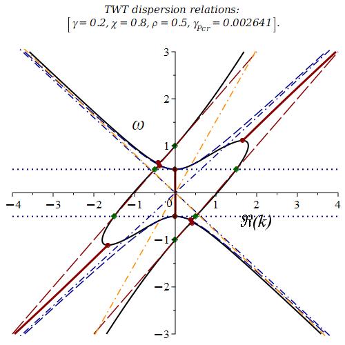
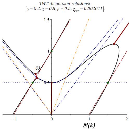
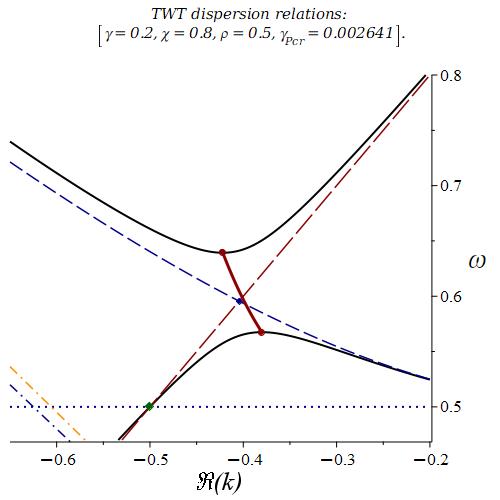
(a)                                               (b)                                               (c)

Figure VIII.1: Dispersion-instability graph and its zoomed fragments for $\chi=0.8$, $\rho=0.5<1$ and $\gamma=0.2>\gamma_{\mathrm{Pcr}}\cong 0.002641$: (a) larger scale version; (b) zoomed fragment of (a); (c) zoomed fragment of (b) for $\Re\left\{k\right\}<0$. Solid (black) curves represent the dispersion curves, dashed (blue) curves represent the dispersion curves for $\gamma=0$ as a reference. Dash-doted straight lines represented high frequency asymptotics for $\gamma=0.7$ (orange) and for $\gamma=0$ (blue). Doted (blue) horizontal straight lines represents points $\left(k,\omega_{\mathrm{c}}\right)$. Diamond (green) dots represent focal points defined by equations (VI.1), diamond (blue) dots represent the cross-points $\mathrm{Gr}_{\mathrm{T}}\bigcap\mathrm{Gr}_{\mathrm{B}}$. The circular dots (red) identify transition to instability points (see Section VIII.1). The bold, solid (red) curves represent branches of points $\left(\Re\left\{k\right\},\omega\right)$ with real $\omega$ and $\Im\left\{k\right\}\neq 0$ which are points of the convection instability.

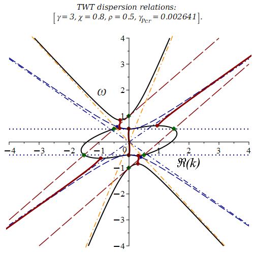
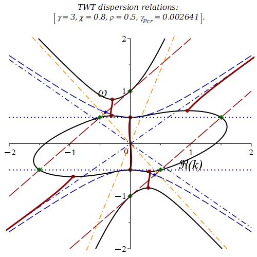
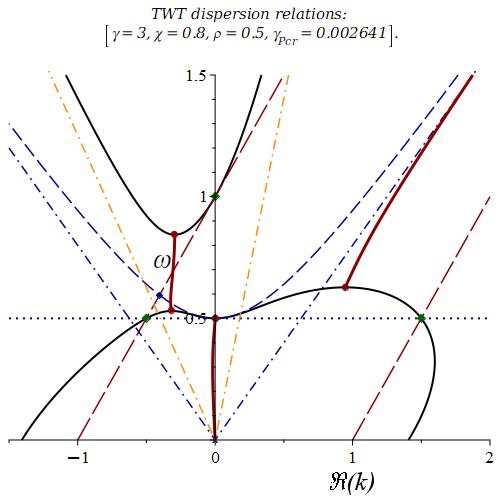
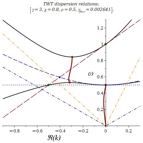
(a)                                                            (b)

Figure VIII.2: Dispersion-instability graph for $\chi=0.8$, $\rho=0.5<1$ and $\gamma=3\gg\gamma_{\mathrm{Pcr}}\cong 0.002641$: (a) larger scale version; (b) zoomed fragment of (a). Solid (black) curves represent the dispersion curves, dashed (blue) curves represent the dispersion curves for $\gamma=0$ as a reference. Dash-doted straight lines represented high frequency asymptotics for $\gamma=0.7$ (orange) and for $\gamma=0$ (blue). Doted (blue) horizontal straight lines represents points $\left(k,\omega_{\mathrm{c}}\right)$. Diamond (green) dots represent focal points defined by equations (VI.1), diamond (blue) dots represent the cross-points $\mathrm{Gr}_{\mathrm{T}}\bigcap\mathrm{Gr}_{\mathrm{B}}$. The circular dots (red) identify transition to instability points (see Section VIII.1). The bold, solid (red) curves represent branches of points $\left(\Re\left\{k\right\},\omega\right)$ with real $\omega$ and $\Im\left\{k\right\}\neq 0$ which are points of the convection instability.

(a)                                                                     (b)

Figure VIII.3: Zoomed fragments of the dispersion-instability graph in Fig. VIII.2 for $\chi=0.8$, $\rho=0.5<1$ and $\gamma=3\gg\gamma_{\mathrm{Pcr}}\cong 0.002641$: (a) zoomed fragment of Fig. VIII.2(b); (b) zoomed fragment of (a). Solid (black) curves represent the dispersion curves, dashed (blue) curves represent the dispersion curves for $\gamma=0$ as a reference. Dash-doted straight lines represented high frequency asymptotics for $\gamma=0.7$ (orange) and for $\gamma=0$ (blue). Doted (blue) horizontal straight lines represents points $\left(k,\omega_{\mathrm{c}}\right)$. Diamond (green) dots represent focal points defined by equations (VI.1), diamond (blue) dots represent the cross-points $\mathrm{Gr}_{\mathrm{T}}\bigcap\mathrm{Gr}_{\mathrm{B}}$. The circular dots (red) identify transition to instability points (see Section VIII.1). The bold, solid (red) curves represent branches of points $\left(\Re\left\{k\right\},\omega\right)$ with real $\omega$ and $\Im\left\{k\right\}\neq 0$ which are points of the convection instability.

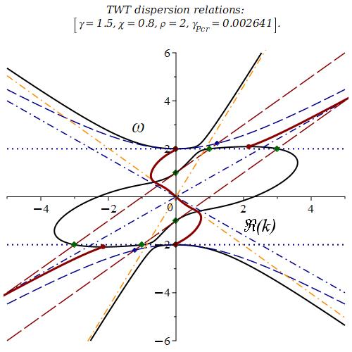
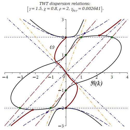
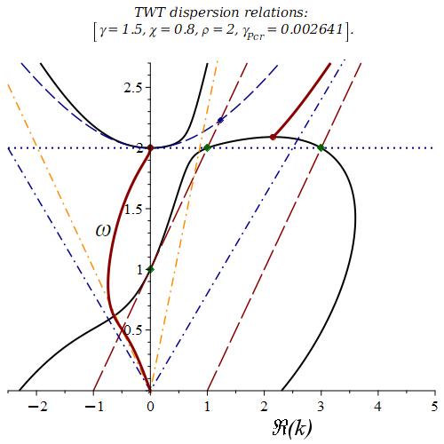
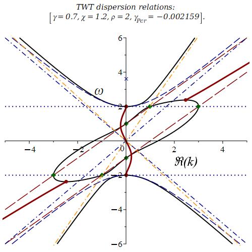
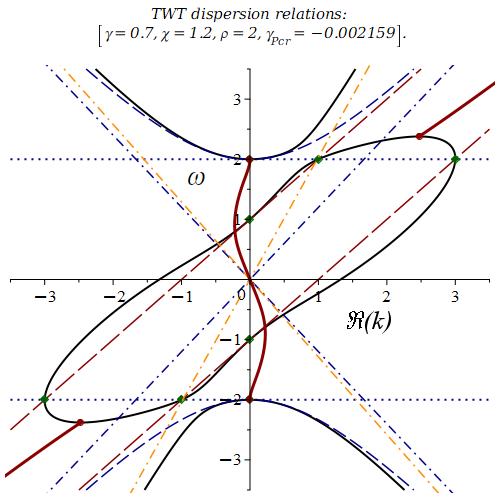
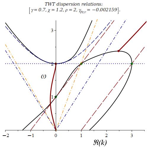
(a)                                           (b)                                               (c)

Figure VIII.4: Dispersion-instability graph and its zoomed fragments for $\chi=0.8$, $\rho=2>1$ and $\gamma=1.3\gg\gamma_{\mathrm{Pcr}}\cong 0.002641$: (a) larger scale version; (b) zoomed fragment of (a); (c) zoomed fragment of (b). Solid (black) curves represent the dispersion curves, dashed (blue) curves represent the dispersion curves for $\gamma=0$ as a reference. Dash-doted straight lines represented high frequency asymptotics for $\gamma=0.7$ (orange) and for $\gamma=0$ (blue). Doted (blue) horizontal straight lines represents points $\left(k,\omega_{\mathrm{c}}\right)$. Diamond (green) dots represent focal points defined by equations (VI.1), diamond (blue) dots represent the cross-points $\mathrm{Gr}_{\mathrm{T}}\bigcap\mathrm{Gr}_{\mathrm{B}}$. The circular dots (red) identify transition to instability points (see Section VIII.1). The bold, solid (red) curves represent branches of points $\left(\Re\left\{k\right\},\omega\right)$ with real $\omega$ and $\Im\left\{k\right\}\neq 0$ which are points of the convection instability.

(a)                                               (b)                                               (c)

Figure VIII.5: Dispersion-instability graph and its zoomed fragments for $\chi=1.2$, $\rho=2>1$ and $\gamma=0.7$: (a) larger scale version; (b) zoomed fragment of (a); (c) zoomed fragment of (b). Solid (black) curves represent the dispersion curves, dashed (blue) curves represent the dispersion curves for $\gamma=0$ as a reference. Dash-doted straight lines represented high frequency asymptotics for $\gamma=0.7$ (orange) and for $\gamma=0$ (blue). Doted (blue) horizontal straight lines represents points $\left(k,\omega_{\mathrm{c}}\right)$. Diamond (green) dots represent focal points defined by equations (VI.1). The circular dots (red) identify transition to instability points (see Section VIII.1). The bold, solid (red) curves represent branches of points $\left(\Re\left\{k\right\},\omega\right)$ with real $\omega$ and $\Im\left\{k\right\}\neq 0$ which are points of the convection instability.

IX Imaginary part of the wave number as a measure of the amplification

The dispersion-instability graphs considered in Section VIII contain only partial information about the instabilities since the information about the imaginary part $\Im\left\{k\right\}$ is suppressed there. In this section we complement dispersion-instability graphs in Section VIII with plots of the imaginary part $\Im\left\{k\left(\omega\right)\right\}$ as a function of real-valued frequency $\omega$. We remind that $\Im\left\{k\left(\omega\right)\right\}$ is responsible for the amplification since the eigenmode dependence of $t$ and $z$ is proportional to $\exp\left\{-\mathrm{i}\left(\omega t-kz\right)\right\}$.

Figures II.7, IX.1, IX.2 and IX.3 show the dependence of the imaginary part $\Im\left\{k\right\}$of the wavenumber $k$ on frequency $\omega$. Note that according to Figures IX.2 and IX.3 operational frequencies and amplitudes of $\Im\left\{k\right\}$ are much higher in the case of $\chi=1.1>1$ compare to the of $\chi=0.9<1$ shown in II.7 and IX.1.

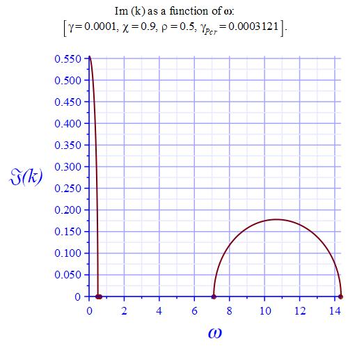
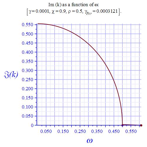
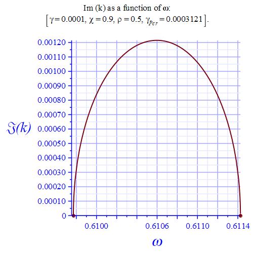
(a)                                               (b)                                               (c)

Figure IX.1: The plot (a) shows the imaginary part $\Im\left\{k\right\}$ of the wavenumber $k=k\left(\omega\right)$ as a function of frequency $\omega$ for $\gamma=0.0001<\gamma_{\mathrm{Pcr}}\cong 0.0003121$, $\chi=0.9<1$ and $\rho=0.5$. The plots (b) and (c) are fragments of the plot (a). Diamond square dots (red) on the $\omega$-axis mark the location of the low and the high frequency cutoffs. Note that in the case there is no high frequency cutoff.

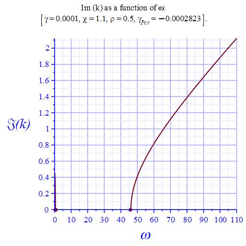
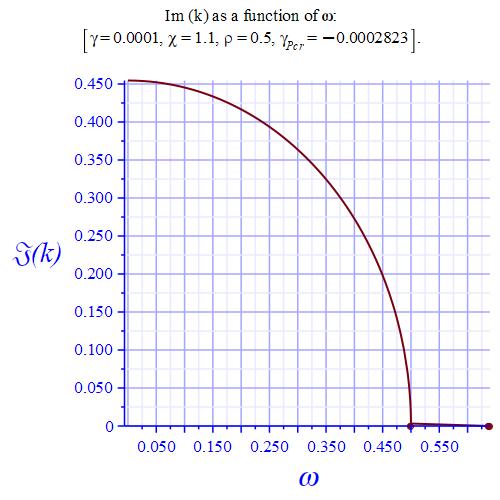
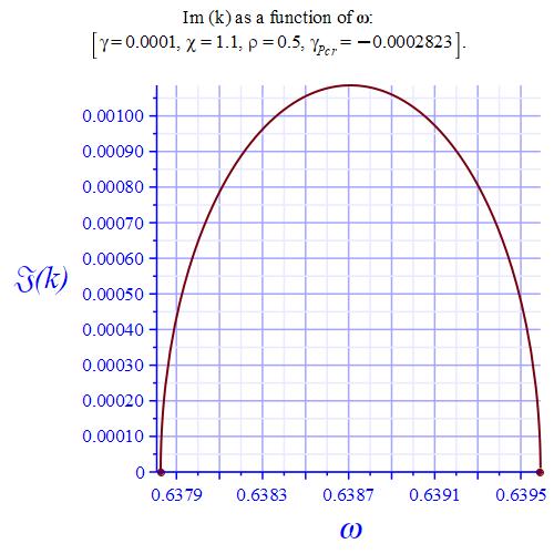
(a)                                               (b)                                               (c)

Figure IX.2: The plot (a) shows the imaginary part $\Im\left\{k\right\}$ of the wavenumber $k=k\left(\omega\right)$ as a function of frequency $\omega$ for $\gamma=0.0001<\gamma_{\mathrm{Pcr}}\cong 0.0003121$, $\chi=1.1>1$ and $\rho=0.5$. The plots (b) and (c) are fragments of the plot (a). Diamond square dots (red) on the $\omega$-axis mark the location of the low and the high frequency cutoffs. Note that in the case there is no high frequency cutoff.

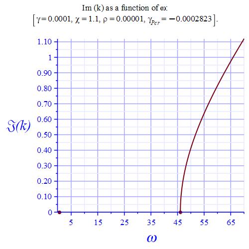
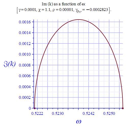
(a)                                                                         (b)

Figure IX.3: The plot (a) shows the imaginary part $\Im\left\{k\right\}$ of the wavenumber $k=k\left(\omega\right)$ as a function of frequency $\omega$ for $\gamma=0.0001<\gamma_{\mathrm{Pcr}}\cong 0.0003121$, $\chi=1.1>1$ and $\rho=0.5$. The plot (b) is fragments of the plot (a). Diamond square dots (red) on the $\omega$-axis mark the location of the low and the high frequency cutoffs. Note that in the case there is no high frequency cutoff.

X Cross-point model for factorized dispersion relations

Our spectral analysis of TWTs suggests that some aspects of the TWT factorized dispersion relations may apply to other systems that might have factorized dispersion relations. With that in mind let us consider a system composed of some two interacting components. Suppose that the dispersion relations for each of this components when they don’t interact in known and the corresponding dispersion relations are defined by the following equations:

$$G_{1}\left(k,\omega\right)=0,\quad G_{2}\left(k,\omega\right)=0.$$ (X.1)

Motivated by the expressions (IV.6), (V.9) of the factorized TWT dispersion relations let us assume that a system composed of some two interacting components satisfying equations (X.1) has the dispersion relation that can be written as follows:

$$G_{1}\left(k,\omega\right)G_{2}\left(k,\omega\right)=\gamma G_{\mathrm{c}}\left(k,\omega\right),$$ (X.2)

where $\gamma$ is the coupling coefficient and to $G_{\mathrm{c}}\left(k,\omega\right)$ as the coupling function. It seems that a special form of equation (X.2) for $G_{\mathrm{c}}\left(k,\omega\right)=1$, that was setup at hoc, appeared in literature but we could not point to a specific reference.

Assuming that the system dispersion relations (X.2) hold we proceed with making more specific assumptions about representation of functions $G_{1}\left(k,\omega\right)$, $G_{2}\left(k,\omega\right)$ and $G_{\mathrm{c}}\left(k,\omega\right)$. Once again, inspired by the factorized TWT dispersion equations (IV.4)-(IV.6) and (V.3), (V.4) we assume that these functions can be completely factorized, that is

$$G_{j}\left(k,\omega\right)\stackrel{{\scriptstyle\mathrm{def}}}{{=}}\prod_{m=1}^{N_{j}}\left(\omega-\omega_{jm}\left(k\right)\right),\quad j=1,2;\quad G_{\mathrm{c}}\left(k,\omega\right)=\prod_{m=1}^{N_{\mathrm{c}}}\left(\omega-\omega_{\mathrm{c}m}\left(k\right)\right),$$ (X.3)

where $N_{1}$, $N_{2}$ and $N_{\mathrm{c}}$ are positive integers, and $\omega_{jm}\left(k\right)$ and $\omega_{\mathrm{c}m}\left(k\right)$ are smooth functions presumed to be known.

The first question that comes to mind is whether one can formulate conditions under which a physical system defined by its Lagrangian would have the dispersion relations that can be written in the factorized form (X.2), (X.3). We admit that answering this question require considerable efforts, and it is outside of the scope of this paper. The reason for introducing general factorized dispersion relations (X.2) is rather for setting up a general framework that can be used to construct a simple approximation to the TWT dispersion equations (V.3), (V.4) in a vicinity of a cross-point as explained in the following section.

X.1 Cross-point model of factorized dispersion relations

Suppose that $\left(\omega_{0},k_{0}\right)$ is a “cross-point” of the graphs of functions $G_{1}$ and $G_{2}$, that a point satisfying the system of two dispersion relations (X.1), namely

$$G_{1}\left(\omega_{0},k_{0}\right)=0,\quad G_{2}\left(\omega_{0},k_{0}\right)=0.$$ (X.4)

Suppose also coupling parameter $\gamma$ to be small, and consider solutions to equation (X.2) in a small vicinity of point $\left(\omega_{0},k_{0}\right)$, that is

$$\left(k,\omega\right)=\left(k_{0}+\delta,\omega_{0}+\delta\right),\quad\left|\delta\right|,\left|\kappa\right|\ll 1,$$ (X.5)

Assuming that equations (X.4) and (X.4) hold and that variables $\gamma$, $\delta$ and $\delta$ are small, that is

$$\left|\gamma\right|\ll 1,\quad\left|\delta\right|\ll 1,\quad\left|\delta\right|\ll 1,$$ (X.6)

we arrive at the following cross-point approximation to the dispersion equation (X.2)

$$\left(g_{1\omega}\delta+g_{1k}\kappa\right)\left(g_{2\omega}\delta+g_{2k}\kappa\right)=\gamma g_{\gamma},$$ (X.7)

where the constants $g_{j\omega}$, $g_{jk}$ and $g_{\gamma}$ are defined by

$$g_{j\omega}=\left(\partial_{\omega}G_{j}\right)\left(\omega_{0},k_{0}\right),\quad g_{jk}=\left(\partial_{k}G_{j}\right)\left(\omega_{0},k_{0}\right),\quad j=1,2;\quad g_{\gamma}=G_{\mathrm{c}}\left(\omega_{0},k_{0}\right).$$ (X.8)

Suppose now that the values of coefficients $g_{j\omega}$, $g_{jk}$ and $g_{\gamma}$ are generic in the sense that functions $g_{1\omega}\delta+g_{1k}\kappa$ and $g_{2\omega}\delta+g_{2k}\kappa$ are linearly independent. Under this assumption we can transform equation (X.7) into a simple special form by the following change of coordinates

$$g_{1\omega}\delta+g_{1k}\kappa=\delta^{\prime}+\kappa^{\prime},\quad g_{2\omega}\delta+g_{2k}\delta=\delta^{\prime}-\kappa^{\prime}.$$ (X.9)

Indeed equation (X.7) can be recast in terms these variables as

$$\delta^{\prime 2}-\kappa^{\prime 2}=\gamma g_{\gamma}.$$ (X.10)

Note now that the graph of equation (X.10) is a hyperbola implying that the graph of original equation (X.7) is a linear transformation of the hyperbola associated with special form (X.10).

In summary, we conclude that generically if the coupling parameter $\gamma$ is small then the graph of the dispersion relations of two interacting systems in a vicinity of the relevant cross-point is a linear transformation of a hyperbola.

In case when $g_{1\omega}\neq 0$ and $g_{2\omega}\neq 0$ we can divide both sides of equation (X.7) by $g_{1\omega}g_{2\omega}$ obtaining the following equivalent equation

$$\left(\delta+g_{1}\kappa\right)\left(\delta+g_{2}\kappa\right)=\gamma g_{\gamma},\quad g_{1}\stackrel{{\scriptstyle\mathrm{def}}}{{=}}\frac{g_{1k}}{g_{1\omega}},\quad g_{2}\stackrel{{\scriptstyle\mathrm{def}}}{{=}}\frac{g_{2k}}{g_{2\omega}},\quad g_{\gamma}\stackrel{{\scriptstyle\mathrm{def}}}{{=}}\frac{g_{\mathrm{c}}}{g_{1\omega}g_{2\omega}}.$$ (X.11)

$$\delta=\omega-\omega_{0},\quad\kappa=k-k_{0}.$$

The equations (X.11) can be viewed as an approximation to the TWT dispersion relation in a small vicinity of point $\left(k_{0},\omega_{0}\right)$.

Motivated by equations ((X.11) we introduce now the following dispersion relations

$$\left(\omega+g_{1}k\right)\left(\omega+g_{2}k\right)=\gamma g_{\gamma},$$ (X.12)

where $g_{1},$$g_{2}$ and $g_{\gamma}$ are given real constant. We refer to dispersion equation (X.12) as the cross-point model dispersion relations. Equation (X.12) can be recast into the following quadratic with respect $\omega$ and $k$ equation

$$\omega^{2}-\left(g_{1}+g_{2}\right)k\omega+g_{1}g_{2}k^{2}-\gamma g_{\gamma}=0.$$ (X.13)

Note that to obtain dispersion relations (X.11) from dispersion relations (X.12) and (X.13) evidently we need to apply the following translation transformation in the $k\omega$-plane

$$\omega\rightarrow\omega-\omega_{0},\quad k\rightarrow k-k_{0}.$$ (X.14)

Quadratic equation (X.13) can readily solved for $\omega$ and $k$ yielding respectively the following representation for cross-model dispersion relations (X.12) and (X.13):

$$\omega=\Omega_{\pm}\left(\gamma,k\right)\stackrel{{\scriptstyle\mathrm{def}}}{{=}}\frac{1}{2}\left[-k\left(g_{1}+g_{2}\right)\pm\sqrt{\left(g_{1}-g_{2}\right)^{2}k^{2}+4\gamma g_{\gamma}}\right],$$ (X.15)

$$k=K_{\pm}\left(\gamma,\omega\right)\stackrel{{\scriptstyle\mathrm{def}}}{{=}}\frac{1}{2g_{1}g_{2}}\left[-\omega\left(g_{1}+g_{2}\right)\pm\sqrt{\left(g_{1}-g_{2}\right)^{2}\omega^{2}+4\gamma g_{1}g_{2}g_{\gamma}}\right].$$ (X.16)

Note that definitions (X.15) and (X.16) of $\Omega_{\pm}$ and $K_{\pm}$ readily imply the following scaling properties of these functions:

$$\Omega_{\pm}\left(s^{2}\gamma,sk\right)=s\Omega_{\pm}\left(\gamma,k\right),\quad K_{\pm}\left(s^{2}\gamma,s\omega\right)=sK_{\pm}\left(\gamma,\omega\right),s>0.$$ (X.17)

These definitions imply also the following inversion symmetry properties

$$\Omega_{+}\left(\gamma,k\right)=-\Omega_{-}\left(\gamma,-k\right),\quad K_{+}\left(\gamma,\omega\right)=-K_{-}\left(\gamma,-\omega\right).$$ (X.18)

Scaling properties (X.17) imply the following identities:

$$\Omega_{\pm}\left(\gamma,k\right)=\sqrt{\gamma}\Omega_{\pm}\left(1,\frac{k}{\sqrt{\gamma}}\right),\quad,K_{\pm}\left(\gamma,\omega\right)=\sqrt{\gamma}K_{\pm}\left(1,\frac{\omega}{\sqrt{\gamma}}\right).$$ (X.19)

Equations (X.19) in turn imply that being given $\gamma>0$ the cross-model dispersion relations (X.12) and (X.13) can be written in the following alternative form:

$$\frac{\omega}{\sqrt{\gamma}}=\Omega_{\pm}\left(1,\frac{k}{\sqrt{\gamma}}\right),\quad\frac{k}{\sqrt{\gamma}}=K_{\pm}\left(1,\frac{\omega}{\sqrt{\gamma}}\right).$$ (X.20)

Note that equations (X.20) manifest a simple scaling property for the graphs of the cross-model dispersion relation as $\gamma$ varies. Indeed, according to equations (X.20) the graph of the cross-model dispersion relation for arbitrary positive $\gamma$ can be obtain from its graph for $\gamma=1$ by the following simple linear scaling transformation by factor $\sqrt{\gamma}$ (see Figures X.3, X.4 and X.5):

$$\omega\rightarrow\sqrt{\gamma}\omega,\quad k\rightarrow\sqrt{\gamma}k$$ (X.21)

Remark 2 (scaling of the cross-point model).

Observe that scaling formula (X.21) shows that two branches of the cross-model dispersion relations written in either form (X.15) or (X.16) are separated by a distance proportional to $\sqrt{\gamma}$. Since evidently $\sqrt{\gamma}\gg\gamma$ for small $\gamma$, one can think of using small coupling of any two systems with a cross point for enhanced sensing, see Remark 1.

Equations (X.15) and (X.16) are useful for our studies of respectively the absolute and the convection instabilities. Consequently, the requirement for $\Omega_{\pm}\left(\gamma,k\right)$ and $K_{\pm}\left(\gamma,k\right)$ defined by equations (X.15) and (X.15 to be real is immediately satisfied if respectively $g_{\gamma}\geq 0$ and $g_{1}g_{2}g_{\gamma}\geq 0$. But in the case when $g_{\gamma}<0$ or $g_{1}g_{2}g_{\gamma}<0$ the $\Omega_{\pm}\left(\gamma,k\right)$ and $K_{\pm}\left(\gamma,k\right)$ are respectively real if and only if the expression under the square root an non-negative, that is

$$\Omega_{\pm}\left(\gamma,k\right)\text{ is real if and only if }\left|k\right|\geq\frac{2\sqrt{\gamma\left|g_{\gamma}\right|}}{\left|g_{1}-g_{2}\right|},\quad g_{\gamma}<0,$$ (X.22)

$$K_{\pm}\left(\gamma,\omega\right)\text{ is real if and only if }\left|\omega\right|\geq\frac{2\sqrt{\gamma\left|g_{1}g_{2}g_{\gamma}\right|}}{\left|g_{1}-g_{2}\right|},\quad g_{1}g_{2}g_{\gamma}<0,$$ (X.23)

Using relations (X.15), (X.22) we may conclude that

$$\Im\left\{\Omega_{\pm}\left(\gamma,k\right)\right\}\neq 0,\text{ for real }k,\text{if and only if }g_{\gamma}<0\text{ and }\left|k\right|\leq\frac{2\sqrt{\gamma\left|g_{\gamma}\right|}}{\left|g_{1}-g_{2}\right|}.$$ (X.24)

In addition to that the following representation holds for complex-valued $\Omega_{\pm}\left(\gamma,k\right)$:

$$\Omega_{\pm}\left(\gamma,k\right)=\frac{1}{2}\left[-k\left(g_{1}+g_{2}\right)\pm\mathrm{i}\sqrt{\left|\left(g_{1}-g_{2}\right)^{2}k^{2}+4\gamma g_{\gamma}\right|}\right],$$ (X.25)

$$\text{ for real }k,\text{ if and only if }g_{\gamma}<0\text{ and }\left|k\right|\leq\frac{2\sqrt{\gamma\left|g_{\gamma}\right|}}{\left|g_{1}-g_{2}\right|}.$$

Evidently relations (X.24) and (X.25) are associated with the absolute instability for wavenumbers in interval $\left|k\right|\leq\frac{2\sqrt{\gamma\left|g_{\gamma}\right|}}{\left|g_{1}-g_{2}\right|}$.

Using relations (X.16), (X.23) we may conclude that

$$\Im\left\{K_{\pm}\left(\gamma,\omega\right)\right\}\neq 0,\text{ for real }\omega,\text{if and only if }g_{1}g_{2}g_{\gamma}<0\text{ and }\left|\omega\right|\leq\frac{2\sqrt{\gamma\left|g_{1}g_{2}g_{\gamma}\right|}}{\left|g_{1}-g_{2}\right|}.$$ (X.26)

In addition to that the following representation holds for complex-valued $K_{\pm}\left(\gamma,\omega\right)$:

$$K_{\pm}\left(\gamma,\omega\right)=\frac{1}{2g_{1}g_{2}}\left[-\omega\left(g_{1}+g_{2}\right)\pm\mathrm{i}\sqrt{\left|\left(g_{1}-g_{2}\right)^{2}\omega^{2}+4\gamma g_{1}g_{2}g_{\gamma}\right|}\right],$$ (X.27)

$$\text{ for real }\omega,\text{ if and only if }g_{1}g_{2}g_{\gamma}<0\text{ and }\left|\omega\right|\leq\frac{2\sqrt{\gamma\left|g_{1}g_{2}g_{\gamma}\right|}}{\left|g_{1}-g_{2}\right|}.$$

Evidently relations (X.26) and (X.27) are associated with the convection instability for frequencies in interval $\left|\omega\right|\leq\frac{2\sqrt{\gamma\left|g_{1}g_{2}g_{\gamma}\right|}}{\left|g_{1}-g_{2}\right|}$.

Figures X.1- X.3 show the plots of the cross-point dispersion relations (X.12) and (X.13) and shaded areas there represent points $\left(k,\omega\right)$ for which at least one of $k$ and $\omega$ becomes complex-valued according to relations (X.25) and (X.27). Figures X.1- X.3 assume efficiently that $\omega_{0}=0$ and $k_{0}=0$ with understanding that in the case of arbitrary real $\omega_{0}$ and $k_{0}$ we need to apply translation transformation (X.12) in the $k\omega$-plane to the relevant graphs.

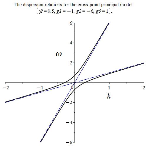
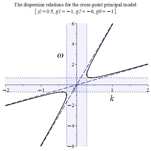
(a)                                                            (b)

Figure X.1: Plots of the cross-point model dispersion relations (X.11) for $\gamma=0.5$, $g_{1}=-1$, $g_{2}=-6$ and (a) $g_{\gamma}=1>0$; (b) $g_{\gamma}=-1<0$. Solid (black) curves represent the dispersion curves for $\gamma=0.5$ whereas dashed (blue) straight lines represent the dispersion curves for $\gamma=0$ as a reference, that is the case when the two subsystems do not interact. The doted (blue) lines identify instability edges and shaded area represent points $\left(k,\omega\right)$ for which at least one of $k$ and $\omega$ becomes complex-valued according to relations (X.25) and (X.27). The circular dots (red) identify the transition to instability points.

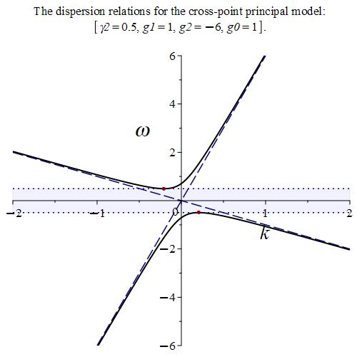
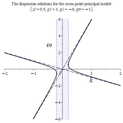
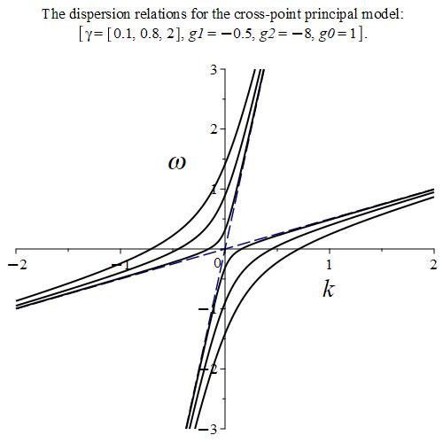
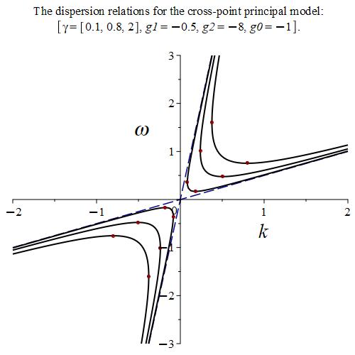
(a)                                                            (b)

Figure X.2: Plots of the cross-point model dispersion relations (X.11) for $\gamma=0.5$, $g_{1}=1$, $g_{2}=-6$ and (a) $g_{\gamma}=1>0$; (b) $g_{\gamma}=-1<0$. Solid (black) curves represent the dispersion curves for $\gamma=0.5$ whereas dashed (blue) straight lines represent the dispersion curves for $\gamma=0$ as a reference, that is the case when the two subsystems do not interact. The doted (blue) lines identify gap edges and shaded area represent points $\left(k,\omega\right)$ for which at least one of $k$ and $\omega$ becomes complex-valued according to relations (X.25) and (X.27). The circular dots (red) identify the transition to instability points.

(a)                                                            (b)

Figure X.3: Plots of the cross-point model dispersion relations (X.11) for $\gamma=0.1,0.8,2$, $g_{1}=-0.5$, $g_{2}=-8$ and (a) $g_{\gamma}=1>0$; (b) $g_{\gamma}=-1<0$. Solid (black) curves represent the dispersion curves for $\gamma=0.1,0.8,2$ whereas dashed (blue) straight lines represent the dispersion curves for $\gamma=0$ as a reference, that is the case when the two subsystems do not interact. The solid curves that are closer to the dashed straight lines correspond to smaller values of coupling coefficient $\gamma$. The circular dots (red) identify the transition to instability points.

Compare Fig. X.3 with Figures VII.2(c), VII.3(c), VII.5(b), VII.6(c), VII.7(b), VII.8(b), (c), VII.9 (c).

X.2 Convection and absolute instability branches

Figures X.4 and X.5 show the dispersion-instability plots that extend plots in Figures X.1(b) and X.1 by adding up there the convection and absolute instability branches. Note that just in case of Figures X.1- X.3 X.4 and X.5 assume efficiently that $\omega_{0}=0$ and $k_{0}=0$ with understanding that in the case of arbitrary real $\omega_{0}$ and $k_{0}$ we need to apply translation transformation (X.12) in the $k\omega$-plane to the relevant graphs.

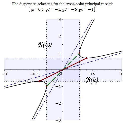
Figure X.4: Dispersion-instability graph of the cross-point model dispersion relations (X.11) for $\gamma=0.5$, $g_{1}=-1$, $g_{2}=-6$ and $g_{\gamma}=-1<0$. Solid (black) curves represent the dispersion curves for $\gamma=0.5$ whereas dashed (blue) straight lines represent the dispersion curves for $\gamma=0$ as a reference, that is the case when the two subsystems do not interact. The doted (blue) lines identify instability edges and shaded area represent points $\left(k,\omega\right)$ for which at least one of $k$ and $\omega$ becomes complex-valued according to relations (X.25) and (X.27). The circular dots (red) identify points of transition from stability to instability. The bold, solid (red) segment represents a branch of points $\left(\Re\left\{k\right\},\omega\right)$ with real $\omega$ and $\Im\left\{k\right\}\neq 0$ which are points of the convection instability described by relations (X.27). The bold dashed (green) segment represents points $\left(k,\Re\left\{\omega\right\}\right)$ with $k$ real and $\Im\left\{\omega\right\}\neq 0$ which are points of the absolute instability described by relations (X.25). The circular dots (red) identify the transition to instability points.

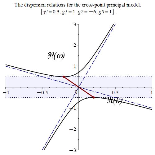
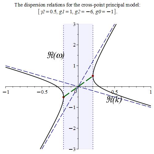
(a)                                                            (b)

Figure X.5: Dispersion-instability graph of the cross-point model dispersion relations (X.11) for $\gamma=0.5$, $g_{1}=1$, $g_{2}=-6$ and (a) $g_{\gamma}=1>0$; (b) $g_{\gamma}=-1<0$. Solid (black) curves represent the dispersion curves for $\gamma=0.5$ whereas dashed (blue) straight lines represent the dispersion curves for $\gamma=0$ as a reference, that is the case when the two subsystems do not interact. The doted (blue) lines identify instability edges and shaded area represent points $\left(k,\omega\right)$ for which at least one of $k$ and $\omega$ becomes complex-valued according to relations (X.25) and (X.27). The circular dots (red) identify points of transition from stability to instability. The bold, solid (red) segment represents a branch of points $\left(\Re\left\{k\right\},\omega\right)$ with real $\omega$ and $\Im\left\{k\right\}\neq 0$ which are points of the convection instability as described by described by relations (X.27). The bold dashed (green) segment represents points $\left(k,\Re\left\{\omega\right\}\right)$ with $k$ real and $\Im\left\{\omega\right\}\neq 0$ which are points of the absolute instability described by relations (X.25). The circular dots (red) identify the transition to instability points.

X.3 Lagrangian framework for the cross-point model

With cross-point model dispersion relations (X.13) in mind let us consider the following form of the dispersion function and the corresponding dispersion relations

$$G_{0}\left(k,\omega\right)\stackrel{{\scriptstyle\mathrm{def}}}{{=}}A\omega^{2}+2\omega kB+Ck^{2}-D,\quad G_{0}\left(k,\omega\right)=0,$$ (X.28)

where $A$, $B$, $C$ and $D$, are real-valued coefficients. The choice of signs before coefficients in equations (X.28) is motivated by its applications to the GTL, the e-beam and other physical systems. Note that equation (X.13) and hence equation (X.28) tacitly assume that $\omega_{0}=0$ and $k_{0}=0$.

It is natural and important to ask if the dispersion relations (X.28) can be associated with a “real physical system”, that is with the Euler-Lagrange equations of a Lagrangian? The answer to this question is positive, and an expression for such a Lagrangian $\mathcal{L}_{G}$ is as follows:

$$\mathcal{L}_{G_{0}}\left(\partial_{t}Q,\partial_{z}Q,Q\right)\stackrel{{\scriptstyle\mathrm{def}}}{{=}}\frac{Q^{2}}{2}G\left(\frac{\partial_{z}Q}{Q},\frac{\partial_{t}Q}{Q}\right)\equiv\frac{1}{2}\left[A\left(\partial_{t}Q\right)^{2}-2B\partial_{t}Q\partial_{z}Q+C\left(\partial_{z}Q\right)^{2}-DQ^{2}\right],$$ (X.29)

where $Q=Q\left(z,t\right)$. Indeed, the EL equations for Lagrangian $\mathcal{L}_{G}$ defined by equations (X.29) are

$$\left[A\partial_{t}^{2}-2B\partial_{t}\partial_{z}+C\partial_{z}^{2}+D\right]Q=0.$$ (X.30)

To find the dispersion relations associated with the EL equation (X.30) we proceed in the standard fashion and consider the system eigenmodes of the form

$$Q\left(z,t\right)=\hat{Q}\left(k,\omega\right)\mathrm{e}^{-\mathrm{i}\left(\omega t-kz\right)}.$$ (X.31)

Plugging in expression (X.30) for $Q\left(z,t\right)$ in the EL equation (X.30) after elementary evaluations we obtain

$$\mathrm{e}^{-\mathrm{i}\left(\omega t-kz\right)}\hat{Q}\left(k,\omega\right)\left[A\omega^{2}+2\omega kB+Ck^{2}-D\right]=0.$$ (X.32)

Assuming naturally that $\hat{Q}\left(k,\omega\right)$ being an amplitude of an eigenmode is not zero we recover from equation (X.32) the following dispersion relation associated with the EL equation (X.30)

$$A\omega^{2}+2\omega kB+Ck^{2}-D=0,$$ (X.33)

which is evidently equivalent to the original dispersion relation (X.28). Hence indeed the Lagrangian $\mathcal{L}_{G_{0}}$ defined by equation (X.29) yields indeed the EL equation having the desired dispersion relation (X.28).

Motivated by the cross-point dispersion relations (X.11) we introduce cross-point dispersion relations

$$G_{\mathrm{crp}}\left(k,\omega\right)\stackrel{{\scriptstyle\mathrm{def}}}{{=}}\left(\omega+g_{1}k\right)\left(\omega+g_{2}k\right)-\gamma g_{\gamma},\quad G_{\mathrm{crp}}\left(k,\omega\right)=0.$$ (X.34)

Then according to formula (X.29) the corresponding to dispersion relations (X.34) Lagrangian $\mathcal{L}_{\mathrm{crp}}$ is of the form

$$\mathcal{L}_{\mathrm{crp}}=\frac{1}{2}\left[\left(\partial_{t}Q+g_{1}\partial_{z}Q\right)\left(\partial_{t}Q+g_{2}\partial_{z}Q\right)-\gamma g_{\gamma}Q^{2}\right].$$ (X.35)

The expression (X.35) can be also readily obtained from the last expression of relations (X.29) by setting up there the following values of coefficients:

$$A=1,\quad B=\frac{g_{1}+g_{2}}{2},\quad C=g_{1}g_{2},\quad D=\gamma g_{\gamma}.$$ (X.36)

Recall that when setting up equation (X.28) we tacitly assumed that $\omega_{0}=0$ and $k_{0}=0$. In case of arbitrary real $\omega_{0}$ and $k_{0}$ representation (X.28) has to be replaced with

$$G\left(k,\omega\right)\stackrel{{\scriptstyle\mathrm{def}}}{{=}}A\left(\omega-\omega_{0}\right)^{2}-2\left(\omega-\omega_{0}\right)\left(k-k_{0}\right)B-C\left(k-k_{0}\right)^{2}-D,\quad G\left(k,\omega\right)=0.$$ (X.37)

We can ask the same question as before. Namely, is the dispersion relations (X.37) can be associated with a “real physical system”, that is with the Euler-Lagrange equations of a Lagrangian? To answer this question we note that the dispersion relation $G\left(k,\omega\right)=0$ turns into the relevant differential operator with respect to variables $t$ and $z$ under substitution

$$\omega\rightarrow-\mathrm{i}\partial_{t}-\omega_{0},\quad k\rightarrow\mathrm{i}\partial_{z}-k_{0}.$$ (X.38)

It is an elementary exercise to compute an expression of that differential operator. It turns out that that expression contains terms $2\mathrm{i}\left(A\omega_{0}+Bk_{0}\right)\partial_{t}$ and $-2\mathrm{i}\left(B\omega_{0}+Ck_{0}\right)\partial_{z}$ which evidently have pure imaginary coefficients, unless $A\omega_{0}+Bk_{0}=B\omega_{0}+Ck_{0}=0$. The presence of these terms rules out a possibility of the existence of a Lagrangian for arbitrary real $\omega_{0}$ and $k_{0}$ unless $A=B=C=0$.

XI Conclusions

We extended here our previously constructed field theory for TWTs as well the celebrated Pierce theory by replacing there the standard transmission line (TL) with its generalization allowing for the low frequency cutoff. We developed all the details of the extended TWT field theory and using a particular choice of the TWT parameters we derived a physically appealing factorized form of the TWT dispersion relations. This form has two factors that represent exactly the dispersion functions of non-interacting generalized transmission line (GTL) and the electron beam (e-beam). We found that the factorized dispersion relations comes with a number of interesting features including: (i) focus points that belong to each dispersion curve as TWT principle parameter varies; (ii) formation of “hybrid” branches of the TWT dispersion curves parts of which can be traced to non-interacting GTL and the e-beam. We also introduced and studied a simple “cross-point model dispersion relation”. This models accounts for the TWT dispersion relation behavior near the cross-points of the dispersion functions of non-interacting GTL and the e-beam when coupling between the GTL and e-beam is small.

ACKNOWLEDGMENT: This research was supported by AFOSR MURI Grant FA9550-20-1-0409 administered through the University of New Mexico. The author is grateful to E. Schamiloglu for sharing his deep and vast knowledge of high power microwave devices and inspiring discussions.

XII Appendix

XII.1 Fourier transform

The several common variations different in signs and constants. Our preferred form of the Fourier transform $\widehat{f}=f^{\land}$ of $f$ and the inverse Fourier transform $f^{\land}$ of $f$ follows to [1, 1.1.7], [2, 20.2], [9, Notations], [16, 7.2, 7.5], [32, 25]:

$$\widehat{f}\left(k\right)\stackrel{{\scriptstyle\mathrm{def}}}{{=}}\int_{-\infty}^{\infty}f\left(z\right)e^{-\mathrm{i}kz}\,dz,\quad f\left(z\right)=\left[\widehat{f}\left(k\right)\right]^{\lor}=\frac{1}{2\pi}\int_{-\infty}^{\infty}\widehat{f}\left(k\right)\mathrm{e}^{\mathrm{i}kz}\,\mathrm{d}k$$ (XII.1)

$$\widehat{f}\left(\omega\right)\stackrel{{\scriptstyle\mathrm{def}}}{{=}}\int_{-\infty}^{\infty}f\left(t\right)e^{\mathrm{i}\omega t}\,\mathrm{d}t,\quad f\left(t\right)=\frac{1}{2\pi}\int_{-\infty}^{\infty}\widehat{f}\left(\omega\right)\mathrm{e}^{-\mathrm{i}\omega t}\,\mathrm{d}\omega,$$ (XII.2)

$$\widehat{f}\left(k,\omega\right)\stackrel{{\scriptstyle\mathrm{def}}}{{=}}\int_{-\infty}^{\infty}f\left(z,t\right)e^{\mathrm{i}\left(\omega t-kz\right)}\,dz\mathrm{d}t,$$ (XII.3)

$$f\left(z,t\right)=\left[\widehat{f}\left(k,\omega\right)\right]^{\lor}=\frac{1}{\left(2\pi\right)^{2}}\int_{-\infty}^{\infty}\widehat{f}\left(k,\omega\right)\mathrm{e}^{-\mathrm{i}\left(\omega t-kz\right)}\,\mathrm{d}k\mathrm{d}\omega.$$

Note the difference of the choice of the sign for time $t$ and spacial variable $z$ in the above formula. It is motivated by the desire to have “wave” form for exponential $\mathrm{e}^{-\mathrm{i}\left(\omega t-kz\right)}$ when both variables $t$ and $z$ are present.

For multi-dimensional space variable $x\in\mathbb{R}^{n}$ the Fourier transform $\widehat{f}$ of $f$ and the inverse Fourier transform $f^{\land}$ of $f$ are defined by, [1, 1.1.7], [9, Notations], [16, 7.5]:

$$\widehat{f}\left(k\right)\stackrel{{\scriptstyle\mathrm{def}}}{{=}}\int_{\mathbb{R}^{n}}\widehat{f}\left(x\right)\mathrm{e}^{-\mathrm{i}k\cdot x}\,\mathrm{d}x,\quad f\left(x\right)=\left[\widehat{f}\left(k\right)\right]^{\lor}=\frac{1}{\left(2\pi\right)^{n}}\int_{\mathbb{R}^{n}}\widehat{f}\left(k\right)\mathrm{e}^{\mathrm{i}k\cdot x}\,\mathrm{d}k,\quad k,x\in\mathbb{R}^{n},$$ (XII.4)

which is consistent with equations (XII.1). Then the Plancherel-Parseval formula reads, [10, 4.3.1], [16, 7.5], [17, 0.26]:

$$\left(f,g\right)=\left(2\pi\right)^{-n}\left(\widehat{f},\widehat{g}\right),\quad\left\|f\right\|=\left(2\pi\right)^{-n/2}\left\|\widehat{f}\right\|,$$ (XII.5)

$$\left(f,g\right)\stackrel{{\scriptstyle\mathrm{def}}}{{=}}\int_{\mathbb{R}^{n}}\overline{f\left(x\right)}g\left(x\right)\,\mathrm{d}x,\quad\left\|f\right\|\stackrel{{\scriptstyle\mathrm{def}}}{{=}}\sqrt{\left(f,f\right)}.$$

This preference was motivated by the fact that the so-defined Fourier transform of the convolution of two functions has its simplest form. Namely, the convolution $f\ast g$ of two functions $f$ and $g$ is defined by Evans 10, 4.3.1, [16, 7.2, 7.5],

$$\left[f\ast g\right]\left(t\right)=\left[g\ast f\right]\left(t\right)=\int_{-\infty}^{\infty}f\left(t-t^{\prime}\right)g\left(t^{\prime}\right)\,\mathrm{d}t^{\prime},$$ (XII.6)

$$\left[f\ast g\right]\left(z,t\right)=\left[g\ast f\right]\left(z,t\right)=\int_{-\infty}^{\infty}f\left(z-z^{\prime},t-t^{\prime}\right)g\left(z^{\prime},t^{\prime}\right)\,\mathrm{d}z^{\prime}\mathrm{d}t^{\prime}.$$ (XII.7)

Then its Fourier transform as defined by equations (XII.1)-(XII.3) satisfies the following properties:

$$\left[f\ast g\right]^{\land}\left(\omega\right)=\widehat{f}\left(\omega\right)\widehat{g}\left(\omega\right),$$ (XII.8)

$$\left[f\ast g\right]^{\land}\left(k,\omega\right)=\widehat{f}\left(k,\omega\right)\widehat{g}\left(k,\omega\right).$$ (XII.9)

XII.2 The Pierce theory concise review

This section is essentially an excerpt from our analysis in SchaFig [29]. The dispersion relation of the Pierce model written in terms of propagation constant $\beta$ reads, Gilm1 [19, Sec. 12.2.2, 12.2.3], [27, 2.2, 2.3]

$$\frac{2C_{\mathrm{P}}^{3}\beta_{\mathrm{e}}}{\left(\beta-\beta_{\mathrm{e}}\right)^{2}}\frac{\beta^{2}\beta_{\mathrm{c}}}{\beta^{2}-\beta_{\mathrm{c}}^{2}}+1=0,\quad\beta=\frac{\omega}{u},\quad\beta_{\mathrm{e}}=\frac{\omega}{\mathring{v}},\quad\beta_{\mathrm{c}}=\frac{\omega}{w},$$ (XII.10)

where $C_{\mathrm{P}}$ is the so-called Pierce gain parameter, $\beta$, $\beta_{\mathrm{e}}$ and $\beta_{\mathrm{c}}$ are wavenumbers (propagation constants) of the eigenmode, the electron beam and the “circuit”, that is, the transmission line, respectively, and $u$, $\mathring{v}$ and $w$ are the corresponding phase velocities. We refer to $\beta$ and to the corresponding

$$\frac{2C_{\mathrm{P}}^{3}\widetilde{\beta}_{\mathrm{e}}}{\left(\beta-\beta_{\mathrm{e}}\right)^{2}}\frac{\beta^{2}\beta_{\mathrm{c}}}{\beta^{2}-\beta_{\mathrm{c}}^{2}}+1=0,\quad\beta=\frac{\omega}{u},\quad\beta_{\mathrm{e}}=\frac{\omega}{\mathring{v}},\quad\beta_{\mathrm{c}}=\frac{\omega}{w},$$ (XII.11)

Equation (XII.10) can be readily transformed into

$$\frac{2\mathring{v}wC_{\mathrm{P}}^{3}}{w^{2}-u^{2}}+\frac{\left(u-\mathring{v}\right)^{2}}{u^{2}}=0,\quad u=\frac{\omega}{\beta},$$ (XII.12)

and we refer to its solutions $u$ as characteristic velocities. The TWT characteristic equation can be viewed as an equivalent representation of the TWT dispersion relations in terms of the phase velocity associated with the relevant TWT eigenmode.

The dimensionless form of equation (XII.12) is

$$\frac{\gamma}{\chi^{2}-u^{\prime 2}}+\frac{\left(u^{\prime}-1\right)^{2}}{u^{\prime 2}}=0,\quad u^{\prime}=\frac{u}{\mathring{v}},\quad\chi=\frac{w}{\mathring{v}},\quad\gamma=2\chi C_{\mathrm{P}}^{3}.$$ (XII.13)

The Pierce theory emerges from the TWT field theory as its high-frequency limit, that is when $\omega\rightarrow\infty$, FigTWTbk [11, Chap. 4.2, 29, 62], with the following characteristic equation in dimensionless form:

$$\mathscr{D}\left(u^{\prime}\right)=\frac{\gamma}{\chi^{2}-u^{\prime 2}}+\frac{\left(u^{\prime}-1\right)^{2}}{u^{\prime 2}}=0,\quad\gamma^{\prime}=\frac{\gamma}{\mathring{v}{}^{2}},\quad u^{\prime}=\frac{u}{\mathring{v}},\quad\chi=\frac{w}{\mathring{v}}.$$ (XII.14)

It can be readily verified that equation (XII.14) is equivalent to equation (XII.13) of the Pierce theory. Note also that equations (XII.13) and (XII.14) are identical if the following relation holds between our TWT principal parameter $\gamma$ and the Pierce gain parameter $C_{\mathrm{P}}$, FigTWTbk [11, Chap. 62]:

$$\gamma=\frac{b^{2}}{C}\frac{e^{2}}{m}R_{\mathrm{sc}}^{2}\sigma_{\mathrm{B}}\mathring{n}=2\mathring{v}wC_{\mathrm{P}}^{3}\;\text{ or }\gamma^{\prime}=\frac{\gamma}{\mathring{v}{}^{2}}=2\frac{w}{\mathring{v}}C_{\mathrm{P}}^{3}=2\chi C_{\mathrm{P}}^{3}.$$ (XII.15)

Note that $C_{\mathrm{P}}^{3}$ is defined as one-quarter of the ratio of the circuit (transmission line) impedance $Z_{0}$ to the e-beam impedance $\frac{V_{0}}{I_{0}}$, [27, Sec. 2.3], [19, Sec. 12.2.2, 12.2.3], FigTWTbk [11, Chap. 62]:

$$C_{\mathrm{P}}^{3}=\frac{Z_{0}I_{0}}{4V_{0}},$$ (XII.16)

where $I_{0}$ and $V_{0}$ are the current and the voltage associated with the e-beam. The quantities used above satisfy the following equations

$$Z_{0}=\sqrt{\frac{L}{C}},\quad I_{0}=e\sigma_{\mathrm{B}}\mathring{n},\quad eV_{0}=\frac{m\mathring{v}^{2}}{2},\quad w=\frac{1}{\sqrt{LC}}.$$ (XII.17)

A straightforward verification confirms the consistency of equations (XII.16) and (XII.17) with equation (XII.15).

XII.2.1 Critical value of parameter $\gamma$ in the Pierce theory

An equivalent form of the characteristic equation (XII.13) for the Pierce model is

$$F\left(u\right)=\frac{\left(u^{2}-{\it\chi}^{2}\right)\left(u-1\right)^{2}}{u^{2}}=\gamma>0.$$ (XII.18)

Fig. provides graphical representation of function $F\left(u\right)$ defined by equations (XII.18) for two cases: $\chi=0.9<1$ and $\chi=1.1>1$. Fig. shows an important difference between the two cases since in equations (XII.18) in $\gamma>0$.

An analysis of the characteristic equation (XII.18) shows that in case when $\chi<1$ there exists a critical value $\gamma_{\mathrm{Pcr}}>0$ of the parameter $\chi$ such that:

1. for $0<\gamma<\gamma_{\mathrm{Pcr}}$ all solutions $u$ to equation (XII.18) are real-valued, there is no amplification;

2. for $\gamma>\gamma_{\mathrm{Pcr}}$ there are exactly two different real-valued solutions $u$ to equation (XII.18) and exactly two different complex-valued solutions that are complex-conjugate, that is there is an amplification.

Consequently, in case when $\chi<1$ the amplification is possible if only if $\gamma>\gamma_{\mathrm{Pcr}}$ and if that is the case it occurs for all frequencies. The critical value $\gamma_{\mathrm{Pcr}}$ and the corresponding to it critical value $u_{\mathrm{Pcr}}$ satisfy the following relations:

$$u_{\mathrm{Pcr}}\left(\chi\right)=\chi^{\frac{2}{3}},\quad\gamma_{\mathrm{Pcr}}\left(\chi\right)=\left.\frac{\left(u^{2}-{\it\chi}^{2}\right)\left(u-1\right)^{2}}{u^{2}}\right|_{u=u_{\mathrm{Pcr}}}=\left(1-\chi^{\frac{2}{3}}\right)^{3}=\left(1-u_{\mathrm{Pcr}}\left(\chi\right)\right)^{3}.$$ (XII.19)

Equations (XII.19) imply that

$$u_{\mathrm{Pcr}}\left(\chi\right)=1-\gamma_{\mathrm{Pcr}}\left(\chi\right)^{\frac{1}{3}}.$$ (XII.20)

Formulas (XII.19) readily imply also that $\gamma_{\mathrm{Pcr}}>0$ if $\chi<1$ whereas $\gamma_{\mathrm{Pcr}}<0$ if $\chi>1,$and

$$\lim_{\chi\rightarrow 1}\gamma_{\mathrm{Pcr}}\left(\chi\right)=0,\quad\lim_{\chi\rightarrow 1}u_{\mathrm{Pcr}}\left(\chi\right)=1.$$ (XII.21)

Hence in the case of $\chi>1$ we have $\gamma_{\mathrm{Pcr}}<0<\gamma$ implying that for any $\gamma>0$ there are always exactly two non-real solutions $u$ to equation (XII.18) and consequently there is always amplification. In contract, in the case $\chi<1$ the amplification exists if and only if $\gamma>\gamma_{\mathrm{Pcr}}>0$.

The value of $\gamma_{\mathrm{Pcr}}\left(\chi\right)$ can be used as natural benchmark unit for given $\chi$. The Fig. XII.1 tabulates the values if $\gamma_{\mathrm{Pcr}}$ for different values of $\chi<1.$

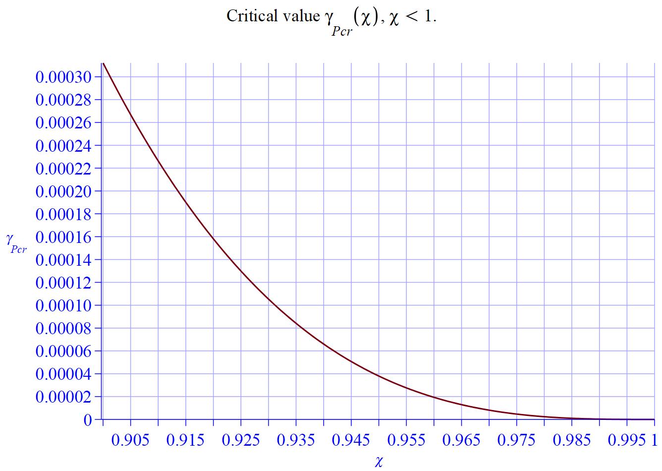
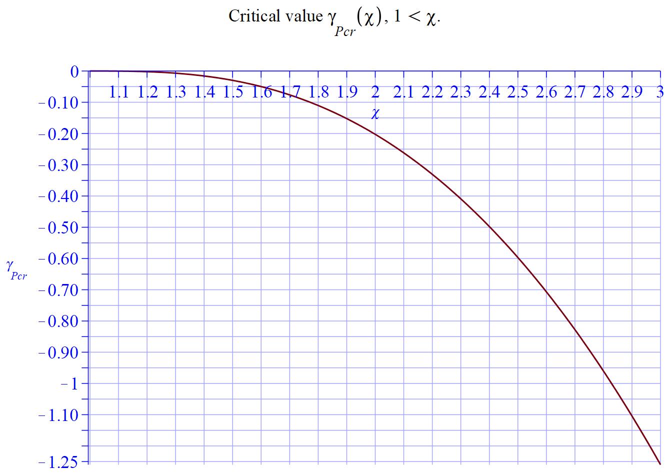
(a)                                                                     (b)

Figure XII.1: The plot of the critical value function $\gamma_{\mathrm{Pcr}}\left(\chi\right)$ defined by formula (XII.19) for : (a) $0.9<\chi<1$; (b) $\chi>1$. Note that $\gamma_{\mathrm{Pcr}}\left(\chi\right)$ is negative for $\chi>1$ implying that always $\gamma>0>\gamma_{\mathrm{Pcr}}\left(\chi\right)$. We remind that the typical values of $\check{\gamma}$ are between $2\cdot 10^{-6}$ and $0.00675$ (see Remark 3).

Remark 3 (typical values of the Pierce parameter and our TWT principal parameter).

For recent studies of the Pierce parameters we refer the reader to [30]. In particular, according [30, Sec. II, p. 3], the typical values of the Pierce parameter $C_{\mathrm{P}}$ are between $0.01$ and $0.15$. Then, in view of relations (XII.15), the corresponding expected typical values of $\check{\gamma}$ are between $2\cdot 10^{-6}$ and $0.00675$.

DATA AVAILABILITY: The data that support the findings of this study are available within the article.

References

- AdamHed [1999] Adams D. and Hedberg L,. Function Spaces and Potential Theory, Springer, 1999.
- ArfWeb [2013] Arfken G. and Weber H., Mathematical Methods for Physicists - A Comprehensive Guide, 7th edn., Academic Press, 2013.
- BBLN [2005] R. Barker., J. Booske, N. Luhmann and G. Nusinovich, Modern Microwave and Millimeter-Wave Power Electronics, Wiley, 2005.
- Brig [1964] R. Briggs, Electron-Stream Interaction with Plasmas, MIT Press, 1964.
- BenSweSch [2016] J. Benford, A. Swegle and E. Schamiloglu, High Power Microwaves, 3rd ed., CRC Press, 2016.
- BraMih [1955] Branch G. and Mihran T., Plasma-frequency Reduction Factors in Electron Beams, IRE Trans.-Electron Devices, April, 3-11, 1955.
- Cart [2018] R. Carter, Microwave and RF Vacuum Electronic Power Sources, Cambridge University Press, 2018.
- Chip [1968] R. Chipman, Transmission Lines, McGraw-Hill Book Co., 1968.
- DauLio1 [2000] Dautray R. and Lions J., Mathematical Analysis and Numerical Methods for Science and Technology, Vol. 1, Physical Origins and Classical Methods, Springer, 2000.
- Evans [1998] Evans L., Partial Differential Equations, AMS, 1998.
- FigTWTbk [2020] A. Figotin, An Analytic Theory of Multi-stream Electron Beams in Traveling Wave Tubes, World Scientific, 2020.
- FigtwtEPD [2021] Figotin A., Exceptional points of degeneracy in traveling wave tubes, J. Math. Phys., 62, 082701 (2021).
- FigMCK [2022] A. Figotin, Analytic theory of multicavity klystrons, Journal of Mathematical Physics, 63, 062703 (2022).
- FigCCTW [2023] A. Figotin, Analytic theory of coupled-cavity traveling tubes, Journal of Mathematical Physics, 64, 042703 (2023).
- FR [2013] A. Figotin and G. Reyes, Multi-transmission-line-beam interactive system, J. Math. Phys., 54, 111901 (2013).
- Foll [1997] Folland G., Fourier analysis and its applications, Princeton Univ. Press, 1992.
- FolPDE [1995] Folland G., Introduction to Partial Differential equations, & Brooks, 1995.
- Franc [1997] Franceschetti G., Electromagnetics, Springer 1997.
- Gilm1 [2011] A. S. Gilmour, Principles of Klystrons, Traveling Wave Tubes, Magnetrons, Cross-Field Amplifiers, and Gyrotrons, Artech House, 2011.
- Gilm [1994] Gilmour A., Principles of Traveling Wave Tubes, Artech House, 1994.
- Kato [1995] Kato T., Perturbation theory for linear operators, Springer 1995.
- MiaMaf [2001] G. Miano and A. Maffucci, Transmission Lines and Lumped Circuit, Academic Press, 2001.
- MilSchw [2006] Milton K. and Schwinger J., Electromagnetic Radiation: Variational Methods, Waveguides and Accelerators, Springer, 2006.
- MAEAD [2019] Minenna D., Andre F., Elskens Y., Auboin J-F., Doveil F., The Traveling-Wave Tube in the History of Telecommunication, Eur. Phys. J., 44(1), 1-36, 2019.
- Pain [2005] H. Pain, The Physics of Vibrations and Waves, 6th ed., Wiley, 2005.
- Pier51 [1951] J. Pierce, Waves in Electron Streams and Circuits, Bell Sys. Tech. Jour., 30, 626-651, (1951).
- PierTWT [1950] J. Pierce, Traveling-Wave Tubes, D. van Nostrand, 1950.
- SchaB [2011] L. Schachter, Beam-Wave Interaction in Periodic and Quasi-Periodic Structures, 2nd ed., Springer, 2011.
- SchaFig [2023] E. Schamiloglu1 and A. Figotin, The Field Theory of Collective Cherenkov Radiation Associated with Electron Beams, arXiv:2310.20152v1 [physics.plasm-ph] 31 Oct 2023.
- Sim17 [2017] D. Simon et.al., On the Evaluation of Pierce Parameters C and Q in a Traveling Wave Tube, Phys. of Plasma, 24, 033114, 2017.
- Stur58 [1958] P. Sturrock, Kinematics of Growing Waves, Phys. Rev., 112(5), 1488-1503, 1958.
- TreB [1975] Treves F., Basic Linear Partial Differential Equations, Academic Press, 1975.
- Tsim [2011] S. Tsimring, Electron Beams and Microwave Vacuum Electronics, Wiley, 2007.
- Wie [2014] Wiersig J., Enhancing the Sensitivity of Frequency and Energy Splitting Detection by Using Exceptional Points - Application to Microcavity Sensors for Single-Particle Detection, Phys. Rev. Lett., 112, 203901 (2014).
- Wie1 [2016] Wiersig J., Sensors operating at exceptional points: General theory, Phys. Rev. A, 93, 033809 (2016).