Near-power-law temperature dependence of the superfluid stiffness in strongly disordered superconductors

Abstract

In BCS superconductors, the superfluid stiffness is virtually constant at low temperature and only slightly affected by the exponentially low density of thermal quasiparticles. Here, we present an experimental and theoretical study on the temperature dependence of superfluid stiffness $\Theta\left(T\right)$ in a strongly disordered pseudo-gaped superconductor, amorphous $\text{InO}_{x}$, which exhibits non-BCS behavior. Experimentally, we report an unusual power-law suppression of the superfluid stiffness $\delta\Theta\left(T\right)\propto T^{b}$ at $T\ll T_{c}$, with $b\sim 1.6$, which we measured via the frequency shift of microwave resonators. Theoretically, by combining analytical and numerical methods to a model of a disordered superconductor with pseudogap and spatial inhomogeneities of the superconducting order parameter, we found a qualitatively similar low-temperature power-law behavior with exponent $b\sim 1.6-3$ being disorder-dependent. This power-law suppression of the superfluid density occurs mainly due to the broad distribution of the superconducting order parameter that is known to exist in such superconductors [1], even moderately far from the superconductor-insulator transition. The presence of the power-law dependence $\delta\Theta\left(T\right)\propto T^{b}$ at low $T\ll T_{c}$ demonstrates the existence of low-energy collective excitations; in turn, it implies the presence of a new channel of dissipation in inhomogeneous superconductors caused by sub-gap excitations that are not quasiparticles. Our findings have implications for the use of strongly disordered superconductors as superinductance in quantum circuits.

I Introduction

Superconducting superinductors, proposed about decade ago [2, 3, 4, 5, 6, 7] as important elements of quantum circuits, now constitute an intensively developing sub-field in the physics of strongly disordered superconductors, as some selected examples [8, 9, 10, 11, 12, 13] demonstrate. Superconducting films used for the construction of superinductors must combine high kinetic inductance per square $L_{K}$ with low dissipation in the microwave frequency range. Large $L_{K}$ corresponds to small 2D superfluid stiffness $\Theta=(2ec/\hbar)^{2}/L_{K}$, and the latter can be achieved close to the Superconducting-Insulator Transition (SIT). The condition of low losses naturally points to a family of superconducting materials in which the SIT occurs without closing the single-particle spectral gap [14]: Indium Oxide [1], Titanium Nitride [15], Niobium Nitride [16], and, possibly, granular Aluminum [17]. Indeed, the absence of low-energy quasiparticles naturally decreases the absorption of microwave electromagnetic field. However, it does not guarantee the absence of other channels of dissipation.

Far away from the SIT, moderately dirty superconductors described by the semiclassical BCS-like theory have a sharp gap $\Delta$ in the excitation spectrum, leading to exponentially low density of quasiparticles at low temperatures, i.e. $n\left(T\right)\propto\exp(-\Delta/T)$. One then expects similar temperature dependence in all other physical quantities, e.g., $\Theta\propto\int dE\,\nu\left(E\right)\,E\,e^{-E/T}\sim T\,n\left(T\right)$. However, such a connection between the DoS and the temperature dependence of $\Theta$ is not observed experimentally at strong disorder. In particular, it was found in Ref. [18] that the temperature dependence of the kinetic inductance per square $L_{K}\propto 1/\Theta$ in strongly disordered TiN films is much stronger than the one predicted within usual Mattis-Bardeen model [19] for the single-electron DoS extracted by Scanning Tunneling Spectroscopy in the same experiment.

In the present paper we report even more striking behavior of the low-temperature suppression of superfluid stiffness, $\delta\Theta(T)=\Theta(0)-\Theta(T)$, in strongly disordered amorphous $\text{InO}_{x}$, as deduced from the dispersion law of one-dimensional plasmon waves in a long superconducting stripe. Namely, we observe the power-law-like temperature dependence $\delta\Theta/\Theta\sim\left(T/T_{0}\right)^{b}$ with $b\sim 1.6-1.7$ and $T_{0}\sim\left(1-7\right)\times 10^{1}\,\text{K}$. This unusual dependence as well as the large magnitude of the effect confidently defy any semiclassical explanation based on mean thermal quasiparticle density.

Addressing $\delta\Theta$ by a semiclassical approach is additionally hindered by the fact that strongly disordered $\text{InO}_{x}$ is known [1, 20] to posses a hard gap $\Delta_{P}\sim 5\text{ K}$ in the single-particle DoS even above the transition temperature $T_{c}\sim 2\text{ K}$. As a result, the electron-hole quasiparticle excitations can be safely neglected at $T\ll T_{c}$ and thus cannot account for the experimentally observed suppression of the superfluid stiffness $\Theta$ with temperature reported in this paper.

To understand the latter, one instead should turn to the properties of the collective modes. While certain contribution to $\delta\Theta$ comes from the aforementioned 1D long-wavelength plasmonic excitations, a simple calculation presented in Section II below quickly demonstrates that the associated effect is too weak at low temperatures. One should thus address the behavior of short-range collective excitations. This latter issue was initially considered within the approximate analytical theory of Ref [21], where it was found that low-energy collective excitations are expected to exist in a broad range of disorder, not necessarily close to the SIT. Unfortunately, the approximation of the space-independent order parameter $\Delta$ employed in Ref. [21] was later found to be to rather crude [22], prompting the issue of short-range low-energy collective modes to be reconsidered.

In the present paper, we show that a proper account of strong inhomogeneity of the order parameter $\Delta(\mathbf{r})$ in a specific model of a pseudo-gaped superconductor allows one to describe near-power-law temperature dependence of the superfluid stiffness $\Theta$, with the order of magnitude of the effect comparable to that in the experimental data. We find that the exponent $b$ of the power law decreases with the increase of disorder, with $b\in(1.5,3)$ in a wide range of disorder parameters. We predict such behavior in a broad range of low temperatures, $\lambda\Delta_{0}\leq T\leq\Delta_{0}/2$, where $\Delta_{0}$ is the typical energy scale of the order parameter, and $\lambda\ll 1$ is the dimensionless Cooper coupling constant. The broad distribution of the order parameter $P(\Delta)$, similar to the one found in Ref. [22], plays a crucial role in our theoretical description. Our theoretical results are in a good qualitative agreement with the experimental data.

The paper is organized as follows: Section II presents the experimental results; Section III formulates the theoretical model; the results of the calculations (both numerical and analytical) are presented in Section IV. Qualitative comparison between experimental and theoretical results, discussions of our findings, and conclusions are present in Section V. The paper is supplemented by a number of Appendices containing various technical details of the analytical approach.

II Suppression of superfluid stiffness in strongly disordered amorphous indium oxide resonators

II.1 Experimental results

The low-temperature evolution of superfluid stiffness in strongly disordered superconductors can be probed experimentally by studying the shift in resonance frequency of a microwave resonator due to the increase of kinetic inductance $L_{K}\propto 1/\Theta$ with temperature [18, 23], a method originally developed for the field of microwave kinetic inductance detectors (MKIDs) [24].

In this work we fabricated open-ended $\lambda/2$ microstrip resonators made from five strongly disordered amorphous indium oxide thin films of different disorder and constant thickness $d=40\leavevmode\nobreak\ \mathrm{nm}$. The film disorder is characterized in situ at cryogenic temperatures using a co-deposited Hall bar and is shown to be increasingly strong, as evidenced by the significant reduction of critical temperature $T_{c}$ and enhancement of normal-state resistance above the superconducting transition. Details of sample disorder are summarized in Table 1. Importantly the disorder range shown here is known to be characterized by the presence of a pseudogap and spatial inhomogeneities of the order parameter [1].

The microwave resonators are long ($L=3.5\leavevmode\nobreak\ \mathrm{mm}$) and narrow ($w=1\leavevmode\nobreak\ \mathrm{\mu m}$) indium oxide strips deposited on a silicon dielectric substrate under which a gold metallic layer acts as a ground plane. Through capacitive coupling to a microwave feedline, a collective motion of Cooper pairs in the resonator can be excited by an AC drive, giving rise to the propagation of plasmon waves with velocity $v=1/\sqrt{lc}$, (where $l$ and $c$ are kinetic inductance and capacitance per unit length respectively) [25, 26, 27].

The open boundary conditions at each ends of the strip lead to Fabry-Pérot-like standing wave resonances with nearly linear dispersion relation $f(k_{n})\sim(1/2\pi)vk_{n}$, where $k_{n}=n\pi/L$ is the wave vector for mode $n$.

The superfluid stiffness of a given $\text{InO}_{x}$ resonator can be extracted from the velocity of plasmons since $v\propto 1/\sqrt{l}\propto\sqrt{\Theta}$. Upon increase of temperature the superfluid density decreases, leading to a decrease of resonance frequency. The evolution of $\Theta(T)$ with temperature can therefore be extracted from the relative frequency shift $\delta f(T)/f=\left[f(20\leavevmode\nobreak\ \mathrm{mK})-f(T)\right]/f(20\leavevmode\nobreak\ \mathrm{mK})\approx(1/2)\,\delta\Theta(T)/\Theta$ defined with respect to the lowest achievable temperature. Further details on the experimental setup and samples can be found in [28].

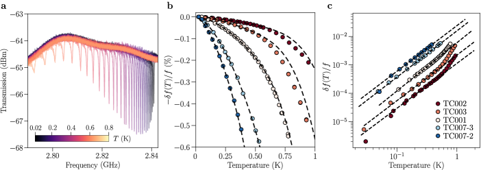
Figure 1: Temperature frequency shift of amorphous indium oxide microwave resonators. a. Transmission resonance as a function of frequency of sample TC007-3 for different temperatures. Upon increasing temperature, the resonance shifts towards lower frequencies. b. Relative frequency shift $\left[f(20\leavevmode\nobreak\ \mathrm{mK})-f(T)\right]/f(20\leavevmode\nobreak\ \mathrm{mK})$ for the five samples of Table 1. The low-temperature part of the data departs from the standard Mattis-Bardeen behavior but can be fitted by adding a power law contribution as in Eq. (1), as shown by the black dashed lines. The power law exponent is $1.57\leq b\leq 1.69$. c. Frequency shift in log-log scale. At the lowest temperatures all curves show a power law with exponent $b\sim 1.6$. Above $0.5\,\text{K}\sim 0.2\leavevmode\nobreak\ T_{c}$ the Mattis-Bardeen mechanism kicks in and the frequency shift retrieves an exponential behavior for the moderately disordered samples (TC002, TC003 and TC001).

The main experimental data are shown in Fig. 1a which displays the transmission as a function of temperature for sample TC007-3. The resonance exhibits a frequency shift upon increasing the temperature from $20\,\text{mK}$ up to $0.8\,\text{K}$. The resulting relative frequency shift $\delta f(T)/f$ is plotted in Fig. 1b together with that of the other four samples listed in Table 1. We readily see that $\delta f(T)/f$ is not exponentially suppressed at low temperatures, in stark contrast with usual BCS dirty superconductors in which the superfluid density is reduced as $\delta\Theta(T)\propto\exp\left\{-\Delta/T\right\}$, due to thermally activated quasiparticles. In log-log scale shown in Fig. 1c, these data exhibit a nearly power-law dependence, $\delta f(T)/f\propto\left(T/T_{0}\right)^{b}$, at the lowest temperature with an exponent $b\sim 1.7$ independent of disorder. This non-BCS power-law dependence of the frequency shift is the central result of this work.

Table 1: Critical temperature, normal-state resistance and zero-temperature superfluid stiffness of disordered indium oxide samples measured in this work. Power law exponent $b$ and temperature scale $T_{0}$ extracted from the temperature-induced frequency shift are also displayed. Where possible, the energy gap $\Delta_{1}$ corresponding to the best fit to Mattis-Bardeen theory at higher temperatures is presented.

Sample	$T_{c}\,(\text{K})$	$R_{n}\leavevmode\nobreak\ \mathrm{(k\Omega/\square)}$	$\Theta(0)\,(\text{K})$	$T_{0}\,(\text{K})$	$b$	$\Delta_{1}\,(\text{K})$
TC002	3.2	1.45	13.3	74.5	1.57	6.8
TC003	2.8	2.0	8.6	45.8	1.60	6.0
TC001	2.2	3.4	4.4	20.5	1.69	4.9
TC007-3	1.6	5.95	1.9	12.9	1.62	–
TC007-2	1.4	7.47	1.4	10.3	1.60	–

Inspecting Fig. 1c in the high temperature range, we see that deviations from this power law with a stronger frequency shift occur for temperatures above about $0.5\,\text{K}$, as shown by the upward curvature of the data in Fig. 1c. We conjecture that these high-temperature deviations most likely relate to the thermally activated quasiparticles and can be phenomenologically described by standard Mattis-Bardeen (MB) theory to account for thermal activation. We thus describe the entire temperature dependence of the frequency shift with:

$$\frac{\delta f(T)}{f}=\left(\frac{T}{T_{0}}\right)^{b}+\left(\frac{\delta f(T)}{f}\right)_{\mathrm{MB}},$$ (1)

where $(\delta f(T)/f)_{\mathrm{MB}}$ is the MB contribution accounting for the high-$T$ deviations. The resulting dashed lines in Fig. 1b fit well data with $b=1.6-1.7$ and $\Delta_{1}\sim 2\leavevmode\nobreak\ T_{c}$, which is a reasonable approximation of the single particle gap for the moderately disordered samples[1]. For the samples TC007-3 and TC007-2 (in blue and light blue on Fig. 1b and c), there is no MB contribution in the measured temperature range.

Interestingly, we found that the $T_{0}$ values resulting from the fits scale linearly with the low temperature superfluid stiffness $\Theta(0)$ that we extracted from the plasmon dispersion of the resonators. Fig. 2 shows $T_{0}$ as a function of $\Theta(0)$ together with a linear fit of slope $5.5$. This particular dependence points to a phase-fluctuation origin of this power law suppression of the frequency shift and thus of the superfluid stiffness.

These experimental observations suggest the existence of low-energy excitations with energies $E\ll T_{c}$ which cannot be captured by the semiclassical BCS-like theory. Indeed, for a given density of bosonic excitation states $\nu\left(E\right)$, the frequency shift is given by $\hbar\delta f\left(T\right)\sim\int dE\,\nu\left(E\right)\,E/\left(e^{\beta E}-1\right)$, so for a power-law dependence of $\delta f(T)\sim T^{b}$ with $b\sim 2$ one needs a finite density of states at $E\sim T$, viz., $\nu\left(E\sim T\right)\sim E^{b-2}$. Otherwise, all thermal effects are exponentially suppressed.

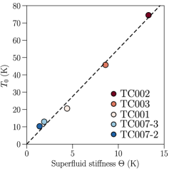
Figure 2: Dependence of the energy scale $T_{0}$ obtained from the fit of the frequency shift with Eq. (1) as a function of the zero-temperature superfluid stiffness $\Theta(0)$. Dashed line is a linear fit indicating that $T_{0}=5.5\leavevmode\nobreak\ \Theta(0)$.

II.2 Thermal excitation of one-dimensional plasma waves

One possible source of low-energy excitations is provided, in principle, by one-dimensional plasmon waves as we discuss below. We first describe the behavior of plasmon excitations at $T=0$, and then calculate the effect of the latter on the superfluid stiffness at low $T$.

It is well known that the application of an electromagnetic drive on a superconductor in the dirty limit leads to a non-linear current-phase relation [29] (see for instance, Eqs. (12-14) in Ref. [29], derived in the framework of the Gor’kov’s equations). For a one-dimensional superconducting wire in the dirty limit and at low frequencies $\omega\ll\Delta$ such non-linearity translates into the appearance of higher-order terms in the expansion of the 2D current density $\boldsymbol{j}_{\text{2D}}$ with respect to vector potential $\boldsymbol{A}$:

$$\boldsymbol{j}_{\text{2D}}=-\frac{\rho_{S}d}{c}\boldsymbol{A}\left(1-\alpha\xi^{2}\left(\frac{2e}{\hbar c}\boldsymbol{A}\right)^{2}\right),$$ (2)

where $\alpha=\frac{\pi}{4}+\frac{3}{4\pi}\approx 1.02$, $\rho_{S}$ is the superfluid density, $d$ is the film thickness, and $\xi$ is the dirty-limit superconducting coherence length. Eq. (2) is analogous to the current-phase relation for a Josephson junction $I(\varphi)=I_{c}\sin\varphi\approx I_{c}\left(\varphi-\varphi^{3}/6\right)$, where $\varphi$ is the superconducting phase-difference across the junction and $I_{c}$ is the critical current.

The Hamiltonian describing long-wavelength plasmons along the wire can be split into two parts: $H=H_{0}+\delta H$. $H_{0}$ is the Hamiltonian related to the linear part of the current-phase relation, and can be diagonalized in a basis of normal modes as $H_{0}=\sum_{n}\hbar\omega_{n}a_{n}^{\dagger}a_{n}$ where $a_{n}^{\dagger}$ and $a_{n}$ are bosonic creation and annihilation operators. The effect of nonlinearity in Eq. (2) translates into the perturbation $\delta H=-\frac{\alpha}{4}\Theta\xi^{2}\int d^{2}\boldsymbol{r}\,|\nabla\varphi|^{4}$, where $\nabla\varphi$ is the superconducting phase gradient.

The relevant part of the Hamiltonian then takes the form (see derivation in F):

$$H_{0}+\delta H=\sum_{n}\hbar\omega_{n}^{\prime}\,a_{n}^{\dagger}a_{n}-\frac{\hbar}{2}\sum_{n,m}K_{nm}\,a_{n}^{\dagger}a_{n}\,a_{m}^{\dagger}a_{m},$$ (3)

with $\omega_{n}^{\prime}=\omega_{n}-\left(K_{nn}+\sum_{m}K_{nm}\right)/4$ being the renormalized frequency, and the Kerr coefficients $K_{nm}$ for the strip geometry defined as

$$K_{nm}=3\alpha\left(1-\frac{1}{4}\delta_{nm}\right)\frac{\xi^{2}}{Lw}\,\frac{\hbar\omega_{n}}{\Theta(0)}\,\omega_{m},$$ (4)

where $\alpha=\frac{\pi}{4}+\frac{3}{4\pi}\approx 1.02$ relates to the strength of the current-phase nonlinearity, $L$ and $w$ are the strip length and width, respectively. Eq. (3) is well-known in quantum optics and is used to describe the interaction of a given mode $n$ with itself (through the self-Kerr coefficient $K_{nn}$), and with another mode $m$ (via the cross-Kerr coefficient $K_{nm}$). The corresponding Kerr effect is seen as the reduction of a normal mode’s frequency due to occupation of other modes:

$$\omega_{n}\to\omega_{n}^{\prime}-\frac{1}{2}\sum_{m}K_{nm}N_{m},$$ (5)

where $N_{m}=\langle a_{m}^{\dagger}a_{m}\rangle$ is the bosonic occupation number of a given normal mode.

A result similar to Eq. (3) for a chain of Josephson junctions can be found in Refs. [30, 31], where authors find a good agreement between experimental and theoretical Kerr coefficients. Both Eq. (4) and the model of [31] with short-range capacitive coupling give the exact same result if one identifies $\Theta(0)$ with the Josephson junction energy $E_{J}$, and $Lw/(2\xi^{2})$ with the number of junctions in he chain $N$, and sets $\alpha=1/6$, corresponding to the coefficient of the cubic term in the expansion of $\sin\varphi$.

We emphasize that the results above are applicable to a homogeneous superconducting strip made of a moderately dirty superconductor in the diffusive limit. The presence of a pseudogap and other non-trivial consequences of strong disorder are, therefore, completely neglected.

We now discuss how one-dimensional plasmons induce a frequency shift as a function of temperature. Upon increase of temperature, the thermal population of plasmonic modes is increased, following the Bose-Einstein distribution $N_{m}=\left[e^{\hbar\beta\omega_{m}}-1\right]^{-1}$, where $\beta=1/k_{B}T$. As a result, the frequency of a given mode $n$ is reduced due to the interaction with other thermally populated modes. Using Eqs. (5) and (4), the total frequency shift with temperature can be expressed as

$$\frac{\delta f(T)}{f}=\frac{3}{2}\alpha\,\frac{\xi^{2}}{Lw}\sum_{m\geq 1}\frac{\hbar\omega_{m}/\Theta(0)}{e^{\hbar\beta\omega_{m}}-1}.$$ (6)

To calculate the sum over modes, the dispersion law $\omega\left(k\right)$ of the plasmonic modes with the wave number $k$ is required, and the latter depends on the electrostatic properties of the system. While generally one expects logarithmic corrections to the linear dispersion law due to long-range Coulomb interaction [26], in the present experimental setup the plasmonic modes with $kh\ll 1$ are not affected due to the screening from the ground plain at distance $h\sim 300\text{ $\mu$m}$, see F for details. For the lowest temperatures, one can thus approximate the plasmonic spectrum by a purely linear dispersion relation, corresponding to $\omega_{m}=m\omega_{1}$, where $\omega_{1}$ is the fundamental mode’s angular frequency. For temperatures higher than $\hbar\omega_{1}/k_{B}$, the sum in Eq. (6) then evaluates to

$$\frac{\delta f(T)}{f}\approx\frac{3}{2}\,\alpha\,\frac{\xi^{2}}{Lw}\,\frac{\hbar\omega_{1}}{\Theta(0)}\,\frac{\pi^{2}}{6}\,\left[\frac{\hbar\omega_{1}}{k_{B}T}\right]^{-2}=\left(\frac{T}{T_{\mathrm{K}}}\right)^{2},$$ (7)

leading to a power-law frequency shift with the temperature scale $T_{\mathrm{K}}$ given by

$$k_{B}T_{\mathrm{K}}=\frac{2}{\pi\sqrt{\alpha}}\,\frac{\sqrt{Lw}}{\xi}\,\sqrt{\Theta(0)\,\hbar\omega_{1}}.$$ (8)

Since $\omega_{1}\propto\sqrt{\Theta(0)}$, $T_{K}$ should scale with the superfluid stiffness as $T_{K}\propto\left[\Theta(0)\right]^{3/4}$. Eq. (7) is applicable while $\hbar\omega_{1}\ll k_{B}T\ll\hbar\omega_{1}\,L/h\sim 10\,\hbar\omega_{1}$, which translates to $0.02\,\text{K}\apprle T\apprle 0.2\,\text{K}$ for the parameters of the present experimental setup. At higher temperatures, the logarithmic corrections to the plasmonic spectrum should be taken into account, resulting in a weak (logarithmic in $T$) enhancement of the effect. Nevertheless, Eq. (7) allows one to correctly estimate the magnitude of the frequency shift due to the plasmonic resonances.

In particular, the estimate Eq. (7) predicts a power-law frequency shift at low temperatures with an exponent $b=2$ close to the experimental value of $\sim 1.6$. However, the magnitude of the effect is much smaller than observed experimentally: using a reasonable estimate for the coherence length in disordered Indium Oxide $\xi\approx 5\,\text{nm}$ [32] and the experimental values of $\Theta(0)$ and $\omega_{1}/(2\pi)\sim 0.4\,\text{GHz}$, one obtains $T_{\mathrm{K}}\sim 3900\,\text{K}$ for the lowest disorder and $T_{K}\sim 1300\,\text{K}$ for the highest disorder, both of which are two orders of magnitude larger than the values of $T_{0}$ observed experimentally (see table 1 and Fig. 2).

We now discuss theoretically how the features of strong disorder can lead to collective modes that suppress the superfluid stiffness at low temperatures.

III Model and Theoretical Approach

In the present section, we outline the theoretical approach that consistently describes the superfluid stiffness $\Theta$ in a strongly disordered superconductor. Subsections III.1 and III.2 present the Hamiltonian of a pseudogapped superconductor and the corresponding current operator; III.3 discusses the problem of macroscopic electromagnetic response of a disordered superconductors and presents a semi-phenomenological connection between $\Theta$ and the statistics of the microscopic current response; III.4 then provides a way to calculate the latter in a particular disorder realization by means of a certain generalization of Belief Propagation, and III.5 describes the numerical procedure for calculating the statistics of the microscopic response. As a result, one obtains a controllable approach to calculate the temperature dependence $\Theta\left(T\right)/\Theta\left(0\right)$ for various disorder strengths.

III.1 Model Hamiltonian

As demonstrated both experimentally [1, 20] and theoretically [33], the materials in question feature localized Cooper pairs even above the transition temperature, whereas the single-particle spectrum exhibits a spectral gap $\Delta_{P}$ several times larger than the bulk transition temperature. Quasiparticle excitation are thus practically absent at low temperatures, and the low-energy physics is governed by hopping of Cooper pairs between localized single-particle states. This can be captured by the following pseudo-spin Hamiltonian:

$$H=-\sum_{i}2\xi_{i}S_{i}^{z}-\sum_{\left\langle ij\right\rangle}4J_{ij}\left(S_{i}^{x}S_{j}^{x}+S_{i}^{y}S_{j}^{y}\right).$$ (9)

Here, $i$ is the index of the single-particle state, $S_{i}^{\alpha}$ are the pseudo-spin operators derived from the fermionic operators as $2S_{i}^{z}=a_{i\downarrow}^{\dagger}a_{i\downarrow}+a_{i\uparrow}^{\dagger}a_{i\uparrow}-1$, $S_{i}^{+}=a_{i\uparrow}^{\dagger}a_{i\downarrow}^{\dagger}$, $S_{i}^{-}=a_{i\downarrow}a_{i\uparrow}$. Then, $\xi_{i}$ are random energies of single-particles states, with probability density at the Fermi level $\xi=0$ expressed in terms of the true single-particle density of states $\nu_{0}$ per spin projection as $P\left(\xi=0\right)=\nu_{0}/n$, with $n$ being the electron concentration, and the summation $\left\langle ij\right\rangle$ goes over all pairs of states that interact due to Cooper attraction with amplitude $J_{ij}$. The latter is given by the corresponding matrix element of the form $J_{ij}=g\intop dr\,\left|\psi_{i}\left(\boldsymbol{r}\right)\right|^{2}\left|\psi_{j}\left(\boldsymbol{r}\right)\right|^{2}$, with $g$ being an interaction constant, and $\psi_{i}\left(\boldsymbol{r}\right)$ corresponding to single-particle wave function of state $i$. While the value of $J_{ij}$ generally vanishes for sites that are localized sufficiently far apart from each other (further than several localizations lengths $\xi_{\text{loc}}$), the randomness of the $\psi_{i}\left(\boldsymbol{r}\right)$ renders the magnitudes of the matrix elements between spatially close states random. To simplify this situation, one adopts three approximations: i) all pairs of states are classified as either strongly interacting or not interacting at all, ii) each state interacts with a large constant number $K+1$ of other states, such that $1\ll K+1\ll N_{\text{loc}}$, with $N_{\text{loc}}=nV_{\text{loc}}$ being the total number of other states available within the localization volume and iii) the interaction amplitude can be replaced by a constant value $J_{ij}=\lambda n/2\nu_{0}K$, where $\lambda\ll 1$ is the dimensionless Cooper coupling constant. While these approximations might seem too crude, a detailed analysis shows [22] that the ignored effects mostly amount to renormalization of physical quantities and inessential corrections, with one notable exception of approximation iii) discussed later. An extended discussion and derivation of this model can be found in [33, 22], while Ref. [34] directly addresses the Superconductor-Insulator Transition in this model.

The proposed structure of interaction matrix elements $J_{ij}$ suggests the notion of interaction graph, in which each single-particle state represents a vertex, while each pair of interacting states $\left\langle ij\right\rangle$ corresponds to an edge. In essence, Hamiltonian (9) reduces the problem to hopping of Cooper pairs (equivalent to hard-core bosons) along this interaction graph, with each site representing a point in real 3D space with some approximate coordinate $\boldsymbol{r}_{i}$ (e.g. the center of mass of the corresponding localized wave function $\psi_{i}$), and each edge $\left\langle ij\right\rangle$ describing the tunneling amplitude between the two “points” $\boldsymbol{r}_{i}$ and $\boldsymbol{r}_{j}$. Crucially, this graph features locally tree-like topology, i.e. for a given site $i$ the neighborhood of size $m_{\text{tree}}\sim\ln N_{\text{loc}}/\ln K\gg 1$ hops along the graph is unlikely to contain any loops, which is the direct consequence of the sparsity of the graph controlled by the parameter $K/N_{\text{loc}}\ll 1$ [35]. As a result, the graph is indistinguishable from a portion of the Bethe lattice as long as any local quantity is concerned, allowing one to apply the rich palette of methods available for analysis of tree-like systems (as done e.g. in Ref. [34]). On the other hand, at distance $r\sim\xi_{\text{loc}}\sqrt{m_{\text{tree}}}\gg\xi_{\text{loc}}$ from a given point $\boldsymbol{r}_{i}$ the actual 3D structure of the model reveals itself via the presence of many loops of length $\geq 2m_{\text{tree}}$ hops containing the chosen site $i$ in the interaction graph. This connection between the structure in the real 3D space and the interaction graph allows one to calculate spatially resolved quantities, as demonstrated e.g. in Ref. [36], where a similar graph model was used in the framework of single-particle Anderson localization problem.

The model (9) possesses a natural superconducting energy scale $\Delta_{0}\approx e^{-1/\lambda}\,n/\nu_{0}$, as explained in [22]. In what follows, all energy quantities in the problem are expressed in units of $\Delta_{0}$. Along with this scale goes the dimensionless disorder strength $\kappa$, also introduced in [22]:

$$\kappa=\frac{\lambda n}{2\nu_{0}\Delta_{0}K}=\frac{\lambda e^{1/\lambda}}{2K}.$$ (10)

We expect that all qualitative properties of the model are defined by physical parameters, such as temperature $T$ and the dimensionless strength of disorder $\kappa$. In particular, the value of other microscopic parameters, such as $\lambda$ and $K$, are not essential as long as the values of $\kappa$ and $T$ (in units of $\Delta_{0}$) are set.

III.2 Current operator

The only possible way to transfer charge in the system described by the Hamiltonian of Eq. (9) is hopping of the Cooper pairs between different states. This implies that the current density operator is described as

$$\boldsymbol{j}\left(r,t\right)=\frac{1}{2}\sum_{e}I_{e}\boldsymbol{D}_{e}\left(r\right),$$ (11)

with the sum going over all directed edges of the interaction graph, hence the factor 1/2. Here, $I_{e}$ is the operator of the current through a given directed edge $e=i\rightarrow j$:

$$I_{e}=2eV_{e}-\frac{4e^{2}}{c}N_{e}A_{e},$$ (12)

where $V_{e}$ plays the role of the velocity operator

$$V_{i\rightarrow j}=J_{ij}\left(S_{i}^{x}S_{j}^{y}-S_{j}^{x}S_{i}^{y}\right),$$ (13)

and the second term represents the diamagnetic contribution to the current:

$$N_{ij}=J_{ij}\left(S_{i}^{x}S_{j}^{x}+S_{i}^{y}S_{j}^{y}\right),$$ (14)

$$A_{e}=\intop d^{3}r\;\left(\boldsymbol{D}_{e}\left(r\right),\boldsymbol{A}\left(r\right)\right)$$ (15)

with $\boldsymbol{A}\left(\boldsymbol{r}\right)$ being the vector potential. Both in $\boldsymbol{j}\left(r\right)$ and in the diamagnetic term, $\boldsymbol{D}_{e}\left(r\right)$ is a short-range vector field that translates the graph topology to the real space, i.e. describes the distribution of the current density $\boldsymbol{j}\left(\boldsymbol{r}\right)$ induced by the process of hopping of a Cooper pair from one site to the other. The exact value of $\boldsymbol{D}_{e}\left(\boldsymbol{r}\right)$ is expressed via the response of the interaction matrix elements $J_{ij}$ to external vector potential and it thus also inherits the randomness of the matrix elements themselves (see III.1). Importantly for us, $\boldsymbol{D}_{e}$ is antisymmetric w.r.t the edge direction, viz. $\boldsymbol{D}_{i\rightarrow j}=-\boldsymbol{D}_{j\rightarrow i}$, and it also obeys the following exact identity due to charge conservation in real space:

$$2\text{div}\boldsymbol{D}_{i\rightarrow j}\left(\boldsymbol{r}\right)=\left|\psi_{i}\left(\boldsymbol{r}\right)\right|^{2}-\left|\psi_{j}\left(\boldsymbol{r}\right)\right|^{2},$$ (16)

where $\psi_{i}\left(\boldsymbol{r}\right)$ are single-particle wave functions.

III.3 Macroscopic superfluid stiffness

We determine the macroscopic superfluid stiffness at low frequencies via the relation $\Theta=\left(\hbar/2e\right)^{2}\rho_{S}d$, where $d$ is the film thickness, and $\rho_{S}$ is the superfluid density entering the London’s equation:

$$\overline{\boldsymbol{j}}=-\frac{1}{c}\rho_{S}\overline{\boldsymbol{A}_{\text{ext}}},\,\,\,\text{div}\boldsymbol{A}_{\text{ext}}=0,$$ (17)

where $\overline{\boldsymbol{A}_{\text{ext}}}$ and $\overline{\boldsymbol{j}}$ are, respectively, the external vector potential and the current density averaged over a macroscopically large region. The current density is, in turn, determined from the response equation at vanishing frequency $\omega\rightarrow 0$:

$$j^{\alpha}=-\intop d^{3}\boldsymbol{r}^{\prime}\,Q_{0}^{\alpha\beta}\left(\boldsymbol{r},\boldsymbol{r}^{\prime}\right)\,A^{\beta}\left(\boldsymbol{r}^{\prime}\right),$$ (18)

with $Q_{\omega}$ being the Fourier transform of the microscopic current response to external vector potential $Q^{\alpha\beta}\left(t-t^{\prime};\boldsymbol{r},\boldsymbol{r}^{\prime}\right)=-\delta\left\langle j^{\alpha}\left(t,\boldsymbol{r}\right)\right\rangle/\delta A^{\beta}\left(t^{\prime},\boldsymbol{r}^{\prime}\right)$. Due to the microscopic disorder, the $Q$ kernel depends on both coordinates $\boldsymbol{r},\boldsymbol{r}^{\prime}$ rather than on their difference $\boldsymbol{r}-\boldsymbol{r}^{\prime}$ and has a nontrivial tensor structure. As a result, the current density induced by the external field $\boldsymbol{A}_{\text{ext}}$ does not automatically satisfy the charge conservation,

$$\text{div}\boldsymbol{j}=0,$$ (19)

so the current $\boldsymbol{j}$ induces additional electromagnetic field $\boldsymbol{A}_{\text{int}}$ such that the current response (18) to the total field $\boldsymbol{A}_{\text{ext}}+\boldsymbol{A}_{\text{int}}$ satisfies Eq. (19).

Consider first the case of weak disorder with diffusive transport in the normal state characterized by $k_{F}l\gg 1,$ where $l$ is the mean free path, and $k_{F}$ is the Fermi wave number. The average current response $\overline{\boldsymbol{j}}$ to a smooth external field $\boldsymbol{A}_{\text{ext}}$ obeying $\text{div}\boldsymbol{A}_{\text{ext}}=0$ already satisfies the charge conservation (19), while the disorder-induced deviation $\delta\boldsymbol{j}=\boldsymbol{j}-\overline{\boldsymbol{j}}$ turns out to be small [37]: $\delta\boldsymbol{j}^{2}/\overline{\boldsymbol{j}}^{2}\sim\frac{\sqrt{\xi_{0}/l}}{k_{F}l}\ll 1$, where $\xi_{0}$ is the zero-temperature coherence length. This allows one to neglect the contribution of $\boldsymbol{A}_{\text{int}}$ to current response and calculate $\rho_{S}$ simply as $\rho_{S}\delta^{\alpha\beta}=c\,\intop d^{3}\boldsymbol{r}^{\prime}\,\overline{Q_{0}^{\alpha\beta}\left(\boldsymbol{r},\boldsymbol{r}^{\prime}\right)}$, where $\overline{\bullet}$ denotes average over disorder, which in this case is carried out by means of the impurity technique [38].

In our model, on the other hand, the statistical and spatial fluctuations $\boldsymbol{j}-\overline{\boldsymbol{j}}$ of the response to a smooth external field are much larger than $\overline{\boldsymbol{j}}$ itself, necessitating a consistent account of the induced field $\boldsymbol{A}_{\text{int}}$. However, we can still assume that the spatial scale at which the total response $\boldsymbol{j}$ convergence to its average value is much smaller than the London’s penetration length $\lambda_{L}=\sqrt{c^{2}/4\pi\rho_{S}}$. In this case, one can neglect the induced magnetic field $B=\text{rot}\boldsymbol{A}_{\text{int}}$ at the relevant length scales, so $\boldsymbol{A}_{\text{int}}$ is dominated by its potential component, viz. $\boldsymbol{A}_{\text{int}}\approx-\frac{c}{i\omega}\nabla\phi$. The current distribution is then described by Eq. (18), where the induced component $\boldsymbol{A}_{\text{int}}$ of total electromagnetic field $\boldsymbol{A}_{\text{ext}}+\boldsymbol{A}_{\text{int}}$ is found self-consistently from the following system of equations:

$$\text{div}\boldsymbol{j}=0,\,\,\,\text{rot}\boldsymbol{A}_{\text{int}}=0,$$ (20)

In particular, due to the assumed division of scales, one can set $\boldsymbol{A}_{\text{ext}}=\overline{\boldsymbol{A}_{\text{ext}}}=\text{const}$. A more detailed derivation of (20) is presented in A.

Due to Eqs. (11) and (16), the problem (18-20) is equivalent to the following discrete system of equations on the values of the onsite electric potential $\phi_{i}$:

$$\sum_{j\in\partial i}I_{i\rightarrow j}=0,\,\,\,E_{i\rightarrow j}=-\left(\phi_{j}-\phi_{i}\right),$$

$$I_{i\rightarrow j}=\frac{c}{i\omega}Q_{ij}\left(\omega=0\right)E_{i\rightarrow j},$$ (21)

with the sum in the first equation going over all neighbors of site $i$, and $Q_{ij}\left(\omega\right)=\intop dt\,e^{i\omega t}Q_{ij}\left(t\right)$ being the Fourier transform of the current response of the graph edge $\left\langle ij\right\rangle$:

$$Q_{ij}\left(t\right)=-\frac{4e^{2}}{c}\left[\left\langle\left[V_{i\rightarrow j}\left(t\right),V_{i\rightarrow j}\left(0\right)\right]\right\rangle-\left\langle N_{ij}\right\rangle\delta\left(t\right)\right].$$ (22)

While one would expect non-local current response $\propto\left\langle\left\langle I_{e}I_{e^{\prime}}\right\rangle\right\rangle$ with $e\neq e^{\prime}$ to be also present in Eq. (21), all such contributions vanish due to locally tree-like structure of the underlying graph, as explained in detail in B. Eq. (21) should be solved for the values of $\phi_{i}$ for all sites $i$ of the system, which then also yields the values of the edge currents $I_{i\rightarrow j}$. The distribution of the electric potential in the real space $\phi\left(r\right)$ and the associated electric field $\boldsymbol{E}\left(\boldsymbol{r}\right)=-\nabla\phi\left(\boldsymbol{r}\right)$ are then restored by inverting the following relation:

$$\phi_{i}=\intop d^{3}r\,\phi\left(r\right)\,\left|\psi_{i}\left(r\right)\right|^{2},$$ (23)

where $\psi_{i}\left(\boldsymbol{r}\right)$ are the single-electron wave functions, see III.1. Upon also computing the current density $\boldsymbol{j}\left(\boldsymbol{r}\right)$ with the help of Eq. (11), one is able to calculate the true superfluid density by means of the last relation in Eq. (20).

One can, however, avoid the procedure of calculating the fields $\phi\left(\boldsymbol{r}\right)$ and $\boldsymbol{j}\left(\boldsymbol{r}\right)$ in real space altogether by noting that Eq. (21) is structurally identical to the Kirchhoff’s law and the Ohm’s law for the interaction graph, with $Q_{ij}c/i\omega$ playing the role of graph edge conductance and $\rho_{S}/i\omega$ corresponding to macroscopic conductance. Macroscopic Ohm’s law then suggests that for a system with the geometry of a brick with macroscopical sizes $L\times w\times d$ the total “conductance” along the $L$ direction is equal to $\Delta\phi/I_{\text{total}}=\left(\rho_{S}/i\omega\right)\,\left(L/wd\right)$, where $I_{\text{total}}$ is the total current through all boundary sites and $\Delta\phi$ is the potential difference between the two boundaries. This constitutes a way to calculate the superfluid stiffness numerically for a given realization of disorder, as done in C.

The resemblance of Eq. (21) to the local Ohm’s law also bears certain physical meaning: according to the second Josephson’s relation, the quantity $\varphi_{i}=-\frac{2e}{\hbar}\phi_{i}/i\omega$ is precisely the superconducting phase of a given site, whereas the last two relations in Eq. (21) express the first Josephson’s relation linearized w.r.t the phase difference. The local structure of Eq. (21) thus becomes a direct consequence of the fact that the system conducts via coherent tunneling of the Cooper pairs.

We are interested in estimating the macroscopic superfluid stiffness analytically, and there are currently no means to do this for a general setting, especially given that the values of the current response $Q_{ij}$ are randomly distributed across many orders of magnitude. However, our numerical experiments on the solution of (21) for 2D systems have shown (see C for details) that the following approximate expression is applicable to our problem for $\kappa\geq 1$:

$$\Theta\left(T\right)\approx C\,\exp\left\{\left\langle\ln Q_{ij}\left(\omega=0\right)\right\rangle\right\}=C\cdot Q_{\text{typ}}\left(T\right),$$ (24)

where $C$ is a prefactor that depends only on the details of the graph structure (such as $K$, $\xi_{\text{loc}}$ and concentration $n$), but not on temperature $T$. As it is explained in E, one can estimate $C\sim nL_{0}^{2}dK$, where $L_{0}\sim\xi_{\text{loc}}$ is the interaction length from III.1, $n$ is site concentration, and $d$ is the thickness of the film. The exact value of $C$ is additionally modified by the presence of short-range correlations in $Q_{ij}$, but this does not change the order of magnitude of the answer, as explained in C. We therefore approximate the temperature change of the superfluid stiffness by that of the typical current response $Q_{\text{typ}}$.

The qualitative origin of the result (24) could be understood by noting that both the original problem (20-18) and its discrete reformulation (21-22) are similar to the problem of macroscopic conductivity of disordered media studied in the seminal paper [39] by A.M. Dykhne. In Ref. [39] it was shown that the macroscopic conductance $\sigma_{\text{eff}}$ of a 2D random medium is equal to the typical value of the microscopic conductance $\sigma_{\text{typ}}=\exp\left\{\left\langle\ln\sigma\left(\boldsymbol{r}\right)\right\rangle\right\}$ provided that $\ln\sigma\left(\boldsymbol{r}\right)$ is distributed symmetrically around its mean value. At first glance, our problem is different: it is three-dimensional, and there are no a priori reasons to assume that either the actual current response $Q_{\omega}^{\alpha\beta}\left(r,r^{\prime}\right)$ or its discrete counterpart $Q_{ij}$ satisfy the requirement on the symmetry of the distribution (although for large enough $\kappa$ the distribution turns out to be sufficiently close to the symmetric log-normal one, as shown in C). However, there are no qualitative reasons for $\Theta$ to differ substantially from the typical current response (at least, in temperature dependence). Indeed, while the calculation of Ref. [39] formally relies on certain duality properties of the 2D problem, it still illustrates the general intuition for the conductance of random media: regions with large conductance can be short-circuited, while regions with small conductance do not conduct at all, rendering the typical conductance to be the only relevant scale of the problem. In the future, we plan to address the validity of the approximate relation (24) in more detail.

III.4 Current response in a given disorder realization

The next step is to calculate the local current response $Q_{ij}$. This is done by means of the extension of the Method of Belief Propagation (BP) to quantum problems. The standard BP scheme is applicable to classical Hamiltonians with discrete local degrees of freedom (e.g. Ising spins). These include several prominent examples in the theory of spin glasses, where the BP method is also known as the cavity method [40, 41]. In essence, BP method tries to accurately describe the structure of local two-point correlations in the Gibbs ensemble, resulting in a system of algebraic self-consistency equations that describe the conditional distributions of one site with respect to the other [42]. Among other things, the BP approach is known to be exact for the systems with tree-like topology, i.e. the ones with no loops in the interaction graph [42].

Remarkably, this latter property is not sensitive to the particular structure of the local degrees of freedom, and a generalization is available to thermal averages of quantum Hamiltonians, such as Eq. (9). The quantum nature of the problem implies replacing the algebraic equations with functional ones, with the latter being analytically intractable in general case. In some cases [43] it is sufficient to characterize the whole problem, in addition to the set of local static fields, by the common intensity of effective quantum noise acting on the spins. In our problem, corrections to the static approximation can be shown to be proportional to small interaction constant $\lambda\ll 1$ and definitely negligible at $\kappa\leq 1$. Although it is not evident that these quantum corrections are irrelevant at large $\kappa$ as well, the numerical analysis provided in Sec. IIIG of Ref. [34] indicates they are weak even very close to SIT. In the present paper we will use static approximation, leaving the account of quantum noise for future work. One can interpret the proposed Approximate Quantum Belief Propagation (AQBP) scheme as the mean field theory of the same type as that of Ref. [22] but with the Onsager reaction terms taken into account, essentially representing the analogue of the classical Thouless-Anderson-Palmer equations [44] for our system.

The central object of the AQBP scheme is the set of local fields $h_{k\rightarrow i}^{\alpha}$ that describe the contribution of spin $k$ to the action of spin $i$, so the latter is described by the effective Hamiltonian:

$$H_{\text{eff}}=-2\xi_{i}S_{i}^{z}+\frac{1}{Z_{i}-1}\sum_{j\in\partial i}2h_{j\rightarrow i}^{\alpha}S_{i}^{\alpha},$$ (25)

where $Z_{i}$ is the number of neighbors of the given site $i$ (equal to $K+1=\text{const}$ within our model). The AQBP provides the self-consistency equations on the values of those fields:

$$h_{k\rightarrow i}^{\alpha}=\sum_{j\in\partial i\backslash\left\{k\right\}}J_{ij}\left\langle 2\hat{S}_{j}^{\alpha}\right\rangle_{j\left(i\right)},\,\,\,\alpha=x,y,$$ (26)

where the summation now goes over all neighbors of $i$ except $k$ (i.e. $K$ summation terms), and $\left\langle 2\hat{S}_{j}^{\alpha}\right\rangle_{j\left(i\right)}$ is the thermal expectation of yet another single-spin Hamiltonian:

$$H_{j\left(i\right)}=-2\xi_{i}\hat{S}_{i}^{z}-2h_{j\rightarrow i}^{x}\hat{S}_{j}^{x}-2h_{j\rightarrow i}^{y}\hat{S}_{j}^{y},$$ (27)

$$\left\langle 2\hat{S}_{j}^{\alpha}\right\rangle_{j\left(i\right)}:=\frac{h_{i\rightarrow j}^{\alpha}}{B_{i\rightarrow j}}\tanh\beta B_{i\rightarrow j},$$ (28)

with $B_{i\rightarrow j}^{2}=\xi_{j}^{2}+\left(h_{i\rightarrow j}^{x}\right)^{2}+\left(h_{i\rightarrow j}^{y}\right)^{2}$.

In order to compute any observable in a given disorder realization, one has to solve this system of algebraic equations for the $h$ fields. In particular, the values of $Q_{ij}$ at frequency $\omega$ are computed as quantum averages over two-spin Hamiltonians that depend on the $h$ fields:

$$\frac{Q_{ij}\left(\omega\right)}{\left(2e\right)^{2}/c}=\sum_{m,n=0}^{3}\left|\left\langle m\left|V_{i\rightarrow j}\right|n\right\rangle\right|^{2}\frac{1}{Z}\frac{\left(\lambda_{n}-\lambda_{m}\right)\left(e^{-\beta\lambda_{n}}-e^{-\beta\lambda_{m}}\right)}{\left(\lambda_{n}-\lambda_{m}\right)^{2}-\left(\omega+i0\right)^{2}}+\sum_{n=0}^{3}\frac{e^{-\beta\lambda_{n}}}{Z}\left\langle n\left|N_{ij}\right|n\right\rangle,\,\,\,Z=\sum_{n=0}^{3}e^{-\beta\lambda_{n}}.$$ (29)

Here $V_{i\rightarrow j}$ and $N_{ij}$ are given by (13) and (14), and $\left\{\lambda_{n},\left|n\right>\right\},\,n=0,1,2,3$ are the eigensystem of the following two-spin Hamiltonian:

$$H_{\left\langle ij\right\rangle} =-\sum_{n=i,j}2\xi_{n}S_{n}^{z}-4J_{ij}\left(S_{i}^{x}S_{j}^{x}+S_{i}^{y}S_{j}^{y}\right)$$

$$-\sum_{\alpha=x,y}\left(2h_{i\rightarrow j}^{\alpha}S_{j}^{\alpha}+2h_{j\rightarrow i}^{\alpha}S_{i}^{\alpha}\right).$$ (30)

At this point we can identify the main reason behind the temperature dependence of $Q_{\text{typ}}$ in Eq. (24). Almost by definition, this quantity is contributed by the most probable disorder configurations. Now, the majority of the disorder configurations have $\left|\xi_{i}\right|,\left|\xi_{j}\right|\gg J,h,T$, hence the spectral problem for Hamiltonian (30) can be addressed perturbatively, rendering $\lambda\approx\pm\xi_{1}\pm\xi_{2}$, with corrections being small as $J/\xi,h/\xi$. As a result, the value of $Q_{ij}$ for such disorder configurations at low temperatures can be estimated as

$$\frac{Q_{ij}}{\left(2e\right)^{2}/c}\approx-2\sum_{n=1}^{3}\frac{\left|\left\langle n\left|V_{i\rightarrow j}\right|0\right\rangle\right|^{2}}{E_{n0}-\left(\omega+i0\right)^{2}/E_{n0}}+\left\langle 0\left|N_{ij}\right|0\right\rangle,$$ (31)

with $n=0$ denoting the ground state, $n>0$ enumerating the excited states, and $E_{n0}=\lambda_{n}-\lambda_{1}\sim E_{F}\gg\Delta_{0},J$. Generally, temperature influences the values of $h$, thus modifying both the matrix elements and the spectral gaps $E_{n0}.$ The latter, however, are only shifted by a quantity of the order $\Delta_{0},J\ll E_{F}$, hence this effect can be discarded along with the frequency dependence, as we are interested in $\omega\sim\Delta_{0}$. The main temperature dependence is thus given by the matrix elements, and by means of the perturbation theory it can be estimated as

$$\frac{Q_{ij}}{\left(2e\right)^{2}/c}\approx\frac{4Jh_{1}h_{2}}{E_{10}E_{20}},$$ (32)

from which it immediately follows that

$$\frac{Q_{\text{typ}}\left(T\right)}{Q_{\text{typ}}\left(T=0\right)}\approx\frac{h_{\text{typ}}^{2}\left(T\right)}{h_{\text{typ}}^{2}\left(T=0\right)}.$$ (33)

To obtain this latter Eq. (33), we used the fact that $h_{i\rightarrow j},h_{j\rightarrow i}$ are all uncorrelated (see below), so the r.h.s of Eq. (33) is expressed via the typical value of the $h$ field. Essentially, this implies that the relative change of the superfluid stiffness mirrors that of the typical order parameter at low temperatures.

III.5 Statistical properties of the current response

According to the Eq. (24), the information about the temperature dependence of the superfluid stiffness is encoded in the statistical distribution of the local current response $Q_{ij}$ in the form of the typical value $Q_{\text{typ}}$. It is thus our aim to compute the average of this quantity over various realizations of disorder. As Eq. (29) suggests, the value of $Q_{ij}$ is expressed via the values of $\xi_{i},\xi_{j}$ on the neighboring sites and on the pair of values $h_{i\rightarrow j},h_{j\rightarrow i}$. Crucially, all four quantities are statistically independent. Indeed, for region of parameters in question, the solution to Eq. (26) is short-correlated due to the large number of summation terms in the right-hand side, as discussed in [22]. As a result, the statistics of $h$ on a given edge does not depend on whether this edge is a part of a tree or a locally tree-like interaction graph that is realized in our case. Iteratively expanding the r.h.s of Eq. (26) then reveals, that these equations possess a directed structure, in contrast to similar equations of Ref. [22]. In other words, the value of $h$ on edge $i\rightarrow j$ gathers statistical information only from the the finite branch rooted at $i$ and not containing edge $i\rightarrow j$ or sites $i$ or $j$. From this, it follows straightforwardly that all four quantities $h_{i\rightarrow j},h_{j\rightarrow i},\xi_{i},\xi_{j}$ are uncorrelated.

As a result, we can substantially simplify the procedure of calculating the value of $Q_{\text{typ}}$: instead of solving the system (26) on a finite size instance of the interaction graph, we can only track the distribution of the $h$ fields with subsequent averaging of the $Q_{ij}$ value (29) over the the distribution of $h$ and $\xi$. The distribution of $h$ can, in turn, be found using the Method of Population Dynamics (MPD), which boils down to claiming that the two sides of Eq. (26) are equal in distribution, which follows from the aforementioned directed structure of Eq. (26) and the short range of correlations in the solution. MPD then allows one to efficiently prepare large number of samples from this distribution: given a large initial pool of $h$ values, one updates each value by replacing it with the value of the r.h.s of Eq. (26), where the values of $\xi$ are sampled randomly for each term, and the values of $h$ are randomly selected from the current pool. After a number of such updates, the pool of $h$ values converges to a large sample from the target distribution. The required number of iterations is not large because the corresponding distribution does not have fat tails in the given range of parameters [22, Sec. III C]. In our implementation, we terminated the process once the mean value $\left\langle h\right\rangle$ has converged. The pool sizes should simply be sufficient to capture the rare events responsible for the formation of the relevant parts of the distribution. In particular, for all simulations presented below, pools of size $10^{7}$ or larger were used to guarantee the convergence of low-value tails of the distribution.

It is worth noting that the assumption of short correlation distance is crucial for this procedure and is not guaranteed in general. In particular, the work [34] analyzes Eq. (26) in the context of the disorder-driven Superconductor-Insulator Transition (SIT) and finds that for $K\leq K_{\text{RSB}}=\lambda\exp\left\{1/2\lambda\right\}$ the distribution of the $h$ fields becomes fat-tailed, and the associated spatial configuration is not at all short-correlated. We are thus interested in the interval $K>K_{\text{RSB}}$, which still contains rich physics, as shown in [22].

IV Theoretical results

IV.1 Numerical results

We start by discussing the qualitative shape of the temperature dependence of the local current response presented on 3. There are three temperature regimes: i) at very low temperatures, one observes exponentially small change in the superfluid stiffness, with the numerical method being unable to properly resolve these values. ii) At moderately low temperatures $T\sim 0.05\,\Delta_{0}-0.3\,\Delta_{0}$ the dependence resembles a power law, although the exponent decreases with temperature. Crucially, the apparent exponent of the power law also decreases with disorder, as shown on 4. iii) At higher temperatures $0.3\,\Delta_{0}\leq T<\Delta_{0}$ the local current response continues to decrease until it vanishes at the transition point. We do not analyze the region of higher temperatures $T\sim\Delta_{0}$, which might also be influenced by quaisparticles due to finite value of the single-particle pseudogap $\Delta_{P}$.

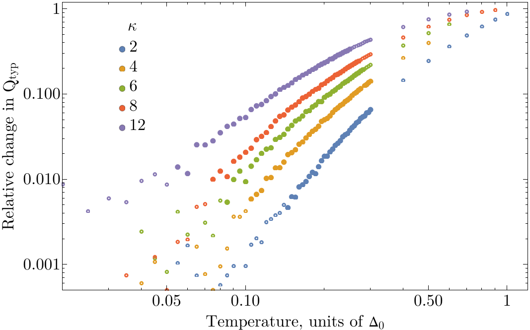
Figure 3: The temperature dependence of the relative change of typical local current response $1-Q_{\text{typ}}\left(T\right)/Q_{\text{typ}}\left(T=0\right)$ in logarithmic scale along both axes for various dimensionless disorder strength $\kappa$ and $K=15$. The temperature is measured in units of $\Delta_{0}$. The points with solid filling are selected according to the empirically chosen criteria $T\in\left[\lambda\left\langle\Delta\right\rangle,\lambda\left\langle\Delta\right\rangle+0.2\Delta_{0}\right]$ with $\left\langle\Delta\right\rangle$ being the mean order parameter at zero temperature. These highlighted points are used for power-law fitting on 4.

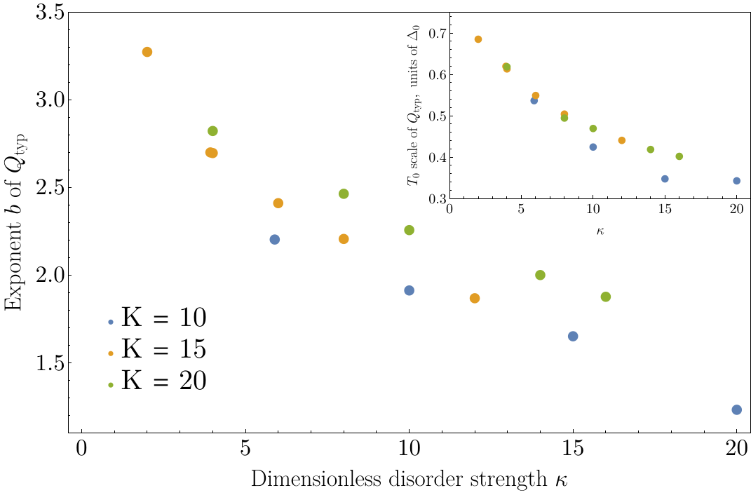
Figure 4: Dependence of the parameters $b$ (main panel) and $T_{0}$ (inset) of the power-law fit $\left(T/T_{0}\right)^{b}$ of the portion of numerical data for $\delta Q_{\text{typ}}\left(T\right)/Q_{\text{typ}}\left(0\right)$. For each set of parameters, the points for fitting are selected according to the empirically chosen criteria $T\in\left[\lambda\left\langle\Delta\right\rangle,\lambda\left\langle\Delta\right\rangle+0.2\Delta_{0}\right]$, with $\left\langle\Delta\right\rangle$ being the mean order parameter at zero temperature, so the dataset for $K=15$ corresponds to highlighted points on 3. The value of $\kappa$ was varied by changing the value of $\lambda$ while keeping $K$ constant, and various colors correspond to various values of $K$.

Another important observation from the numerical results is that the relative change in the typical current response $\delta Q_{\text{typ}}/Q_{\text{typ}}$ goes in line with that of the mean order parameter $\delta\left\langle\Delta\right\rangle/\left\langle\Delta\right\rangle$. In particular, it is true that

$$\frac{\delta\left\langle\Delta\right\rangle/\left\langle\Delta\right\rangle}{\delta Q_{\text{typ}}/Q_{\text{typ}}}=0.5\pm 0.05,$$ (34)

for all points highlighted on 3, regardless of the model parameters. This result is in agreement with the qualitative prediction (33), as our numerical experiments show that $\Delta_{\text{typ}}$ and $\left\langle\Delta\right\rangle$ differ by a temperature-independent factor. In addition, this numerical relation is roughly consistent with the result of Ref. [45], where the relation $\rho_{S}\propto\Delta^{2}\sim h^{2}$ is claimed. While our numerical experiments clearly imply that such a relation does not hold literally, it is apparently correct as far as the relative temperature variations are concerned. Eq. (34) then allows us to calculate the temperature dependence of $Q_{\text{typ}}$ from that of $\left\langle\Delta\right\rangle$. The latter, as it turns out, is amenable for analytical description.

IV.2 Analytical analysis of low-$T$ behavior

While calculating $Q_{ij}$ requires diagonalization of the two-spin Hamiltonian (30), the order parameter $\Delta$ is almost directly accessible from the statistics of the $h$ fields. Indeed, from (25) and (26) one obtains:

$$\Delta_{i}=\sum_{j\in\partial i}J_{ij}\left\langle 2\hat{S}_{j}^{\alpha}\right\rangle_{j\left(i\right)},$$ (35)

which coincides with the Eq. (26) for $h$ itself for up to the difference in the summation number of terms in the r.h.s ($K+1$ instead of $K$).

In what follows, we will compute the expectation $\left\langle h\right\rangle$ of the $h$ field, which coincides with the average order parameter $\left\langle\Delta\right\rangle$ up to an insignificant factor $\left(K+1\right)/K$, as can be seen from Eq. (35). At the cost of additional technical effort, our theory also allows us to calculate the typical value $h_{\text{typ}}=\exp\left\{\left\langle\ln h\right\rangle\right\}$, which is more relevant for the value of the superfluid stiffness according to Eq. (33). However, this appears to be unnecessary: the statistical data for the $h$ field obtained by the MPD (see III.5) demonstrates that the relation $\left\langle h\right\rangle/h_{\text{typ}}$ is nearly temperature-independent up until the transition region $T\sim\Delta_{0}$. This also explains why we chose to use the mean value of $\left\langle\Delta\right\rangle$ rather than the typical value $\Delta_{\text{typ}}$ in the numerical relation (34): the former is easier to calculate analytically while being proportional to the latter with a nearly temperature-independent coefficient in the relevant range of temperatures.

The distribution of $h$ fields can be computed straightforwardly by means presented earlier in [22], although the calculations are considerably simpler due to the absence of the self-action. Indeed, the work [22] dealt with the necessity to disentangle the mutual correlation between the values of $\Delta$ on neighboring sites due to their equivalence in the self-consistency equation. On the other hand, the value of $h_{j\rightarrow i}$ only collects information about the values of $\xi_{k}$ and $h_{l\rightarrow m}$ in one direction (safe for the present of loops, that, however, do not influence the value of $h$ due to rapid decay of correlations with distance on the graph), This feature has made this problem amenable to the MPD in the first place, and the latter is equivalent to claiming that the two sides of the Eq. (26) are equal in distributional sense, with all random variables in the r.h.s being statistically independent:

$$P_{h}\left(h\right)=\prod_{k=1}^{K}\intop_{0}^{\infty}P_{h}\left(h_{k}\right)dh_{k}\int P_{\xi}\left(\xi_{k}\right)d\xi_{k}\cdot\delta\left(h-\frac{\lambda}{K}\sum_{k=1}^{K}f\left(h_{k},\xi_{k}\right)\right),$$ (36)

where $f\left(h_{k},\xi_{k}\right)$ is the spin average in the r.h.s of Eq. (26). As soon as the equation on distribution of $h$ is obtained in such a way, the approach described below is similar to that of [22]. In particular, at zero temperature one finds for the cumulant generating function $m\left(s\right)$:

$$m\left(s\right):=\ln\left\langle e^{ish}\right\rangle=is\left\langle h\right\rangle+\frac{\lambda\left\langle h\right\rangle}{\kappa}F\left(\kappa s\right),\,\,\,\text{Im}s\ll e^{1/\lambda},$$ (37)

$$F\left(\sigma\right)=\intop_{0}^{1}dw\frac{e^{i\sigma w}-1-i\sigma w}{w^{2}\sqrt{1-w^{2}}},$$ (38)

with $\left\langle h\right\rangle$ determined self-consistently from

$$\left\langle h\ln h\right\rangle=0.$$ (39)

Here, the l.h.s is calculated by using the expression (37) for $m\left(s\right)$, thus representing a function of $\left\langle h\right\rangle$, and Eq. (39) has to be solved for $\left\langle h\right\rangle$. In the same way, one can show that the statistics of the order parameter is described by the following generating function:

$$\ln\left\langle\exp\left\{is\Delta\right\}\right\rangle=\frac{K+1}{K}m\left(s\right),$$ (40)

and we once again remind that both $h$ and $\Delta$ are now measured in units of $\Delta_{0}$. We are interested in $K\gg 1$, hence the prefactor in front of $m$, arising from the different number of summation terms in Eqs. (26) and (35), can be discarded.

It is expected that any effect that is larger than the BCS-like exponential dependence of the form $e^{-2\left\langle\Delta\right\rangle/T}$ will be produced by anomalously low values of the order parameter (the unusual factor 2 in the exponent is due to the absence of single-electron quasiparticles in our model). In other words, we are interested in the probability of the order parameter $\Delta$ and the $h$ field to attain values of the order of temperature, with latter being much smaller than mean order parameter $\left\langle\Delta\right\rangle$. Quantitatively, the extreme value statistics of $h$ is encoded in the asymptotic of the $m$ function at $s=it,t\gg 1$, as shown in [22]. This asymptotic is given by

$$m\left(it\right)\approx-At+Bt\ln t,\,\,\,1\ll t\ll t^{*}\sim e^{A/B-1},$$ (41)

$$A=\left\langle h\right\rangle\left\{1-\lambda\left[\gamma-1+\ln 2\kappa\right]\right\},\,\,\,B=\lambda\left\langle h\right\rangle,$$ (42)

where $\gamma=0.577...$ is the Euler-Mascheroni constant, and the estimation for $t^{*}$ follows from the fact that expression (41) is only valid until it no longer represents a decreasing function. The distribution function $P\left(h\right)$ for $h<\left\langle h\right\rangle$ behaves as follows:

$$P\left(h\right)\approx\sqrt{\frac{\zeta\left(h\right)}{2\pi B^{2}}}\exp\left\{-\zeta\left(h\right)\right\},$$ (43)

$$\zeta\left(h\right)=B\exp\left\{\frac{A-h}{B}-1\right\}.$$ (44)

For instance, at $T=0$, one uses Eq. (42) to obtain $\zeta\left(h\right)=\frac{\lambda\left\langle h\right\rangle e^{-\gamma}}{2\kappa}\exp\left\{\frac{1}{\lambda}\left(1-h/\left\langle h\right\rangle\right)\right\}$. Note that while the exponent in $\zeta\left(h\right)$ features a large factor $\sim 1/\lambda\gg 1$, the prefactor $\sim\lambda\left\langle h\right\rangle/2\kappa$ in front of this exponent is actually small in the region of interest, rendering the probability density (43) a complicated function of $h$.

Eq. (43) ceases to work at sufficiently small $h$, where the relevant value of $t$ exceeds $t^{*}$, rendering Eq. (41) inapplicable. This corresponds to $\zeta\left(h\right)$ reaching the value of $Bt^{*}$, which happens at

$$h\sim h_{\min}=B=\lambda\left\langle h\right\rangle.$$ (45)

Physically, $h_{\min}$ plays the role of the minimum value of the $h$ field in the sense that the average $\left\langle e^{-2h/T}\right\rangle$ for $T\ll 2h_{\min}$ is essentially given by $e^{-2h_{\min}/T}$, which can also be expressed by the following description of the $m$ function for $t\geq t^{*}$ :

$$m\left(it\right)\sim-h_{\min}t,\,\,t\gg t^{*}.$$ (46)

The value of $h_{\min}$ is then consistent with the continuity of $m$, i.e. the values of $m\left(it^{*}\right)$ given by the two asymptotic expressions (41) and (46) coincide.

We also note that the expression (41) is only valid for sufficiently weak fluctuations of the interaction matrix elements $J_{ij}$ of the original Hamiltonian (9), viz. $\delta J/J\ll\sqrt{\lambda/\kappa}$ [22], whereas our model assumes $J_{ij}=\text{const}$ for all connected sites (see approximation iii) in III.1).

The same analysis that lead to Eq. (37) shows that for finite temperatures the value of $m\left(it\right)$ acquires a correction

$$\delta m\left(it\right)\approx+\lambda t\frac{\partial}{\partial\beta}\intop_{0}^{1}dw\frac{e^{m\left(2i\beta/w\right)}}{\sqrt{1-w^{2}}},$$ (47)

which is produced by the leading term in the expansion of $\tanh\beta\sqrt{\xi^{2}+\Delta^{2}}$ in Eq. (28) in powers of $\exp\left\{-2\beta\sqrt{\xi^{2}+\Delta^{2}}\right\}$. As already anticipated, the integral in the r.h.s is only sensitive to the asymptotic of the $m$ function at $s=it,t\gg 1$. The correction itself amounts to renormalization of the $A$ coefficient in Eq. (41):

$$A\left(T\right)-A\left(0\right)=-\lambda\frac{\partial}{\partial\beta}\intop_{0}^{1}dw\frac{e^{m\left(2i\beta/w\right)}}{\sqrt{1-w^{2}}}.$$ (48)

Eq. (39) for the value of $\left\langle h\right\rangle$ also changes to

$$\left\langle h\ln h\right\rangle\approx+\frac{\partial}{\partial\beta}\intop_{0}^{1}dw\frac{e^{m\left(2i\beta/w\right)}}{\sqrt{1-w^{2}}},$$ (49)

and contains exactly the same $w$ integral as the one in (48). One has to solve the new equation for $\left\langle h\right\rangle$, similarly to the zero-temperature case.

It is then natural to replace $m\left(it\right)$ in Eqs. (48-49) with its intermediate asymptotic expression (41) to obtain a closed system of equations on $A$ and $B=\lambda\left\langle h\right\rangle$. The emerging divergence of the integrals at small values of $w$ should be cut at $w\sim w^{*}=2\beta/t^{*}$, in accordance with the limit of applicability of the intermediate asymptotic (41). The remaining region $w\leq w^{*}$ produces an exponentially small contribution because for $t\geq t^{*}$ the value of $e^{m\left(it\right)}$ is exponentially small: $e^{m\left(it\right)}\sim e^{-h_{\text{min}}t}\ll 1$. If the temperatures are also exponentially small, i.e. $T\leq T^{*}=2/t^{*}=e^{\gamma}e^{-1/\lambda}/\kappa\ll 1$ one obtains $w^{*}\geq 1$, so a more accurate calculation of the $w$ integral has to be performed in this case. However, the same Eq. (46) still implies that the value of the $w$ integrals is of the order of $e^{-2h_{\min}/T}\leq e^{-h_{\min}t^{*}}\ll 1$, implying an exponentially small change in all physical quantities, which is consistent with the numerical data on 3.

We also note that Eqs. (47-49) are applicable while the approximation $1-\tanh x\approx 2e^{-2x}$ is applicable for the typical values of $x=\beta\sqrt{\xi^{2}+h^{2}}$, which is true for $T\leq T_{\max}\sim 2\left\langle h\right\rangle$.

The qualitative behavior of the solution to Eqs. (48-49) can be understood by employing the direct perturbation theory in $T$. Namely, one treats the change in $A$ and $\left\langle h\right\rangle$ as a perturbation, and the leading order of the latter is given by:

$$\delta h\propto I\left(T\right)=\frac{\partial}{\partial\beta}\intop_{w^{*}}^{1}dw\frac{e^{-A\frac{2\beta}{w}+B\frac{2\beta}{w}\ln\frac{2\beta}{w}}}{\sqrt{1-w^{2}}},\,\,w^{*}=\frac{2}{T}e^{1-A/B},$$ (50)

where the values $A,B$ are taken at $T=0$, i.e. from (42), and the omitted positive coefficient of proportionality is temperature-independent (but does depend on $\kappa,\lambda$). The r.h.s of this equation is negative, and the plot of its absolute value for a reasonable choice of the parameters is shown on 5. It clearly indicates the same type of power-law-like behavior as the one shown on 3, although the power varies with $T$, as can be see e.g. by the values of the log-derivative $d\ln I/d\ln T$.

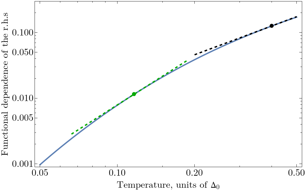
Figure 5: Temperature dependence of the r.h.s of (50) for $\left\langle h\right\rangle=0.46,\,\,\kappa=10,\,\,\lambda=0.123$. The dashed straight lines visualize the log-derivative $b=d\ln I\left(T\right)/d\ln T$, green: $T=T_{\min}=2\lambda\left\langle h\right\rangle$, $b=2.48$, black: $T=0.4$, $b=1.46$.

The comparison of the approximate theory with the numerical calculation by means of the MPD is shown on 6 and is rather satisfying. Discrepancies are only visible at high temperature, where the expressions (47-49) are no longer applicable due to higher powers of $e^{-\beta x}$ in the low-temperature expansion of $\tanh\beta x$. This theory allows us to give more quantitative description to the claims above:

1. At low temperatures $T\leq T_{\max}\sim\left\langle\Delta\right\rangle$ the temperature dependence of the superfluid stiffness $\delta\Theta\left(T\right)=\Theta\left(T=0\right)-\Theta\left(T\right)$ follows that of the mean order parameter:

   $$\frac{\delta\Theta\left(T\right)}{\Theta\left(T=0\right)}\approx 2\,\frac{\delta\left\langle\Delta\right\rangle\left(T\right)}{\left\langle\Delta\right\rangle\left(T=0\right)}$$ (51)

2. For $\lambda\left\langle\Delta\right\rangle\sim T_{\min}\leq T\leq T_{\max}\sim\left\langle\Delta\right\rangle$ a complicated profile of the temperature dependence of the superfluid stiffness is observed. It can be roughly described by a power law

   $$\frac{\delta\Theta}{\Theta}\approx\frac{\delta Q_{\text{typ}}}{Q_{\text{typ}}}\approx 2\frac{\delta\left\langle\Delta\right\rangle}{\left\langle\Delta\right\rangle}\sim\left(T/T_{0}\right)^{b},$$ (52)

   although the power $b$ gradually decreases with $T$, which also allows other descriptions of the data (see D). The common trend is that $b$ decreases with disorder strength $\kappa$. The qualitative shape of the dependence is described by the integral of the form (50). We also note that our analysis suggests that the shape of this dependence is sensitive to certain details of the microscopic model as the latter determine the statistics of low values of the order parameter.

3. At $T\leq T_{\min}$ the dependence of all physical quantities on temperature roughly follows an activation profile:

   $$\frac{\delta\Theta}{\Theta}\approx\frac{\delta Q_{\text{typ}}}{Q_{\text{typ}}}\approx 2\frac{\delta\left\langle\Delta\right\rangle}{\left\langle\Delta\right\rangle}\sim\exp\left\{-\frac{2T_{\min}}{T}\right\}.$$ (53)

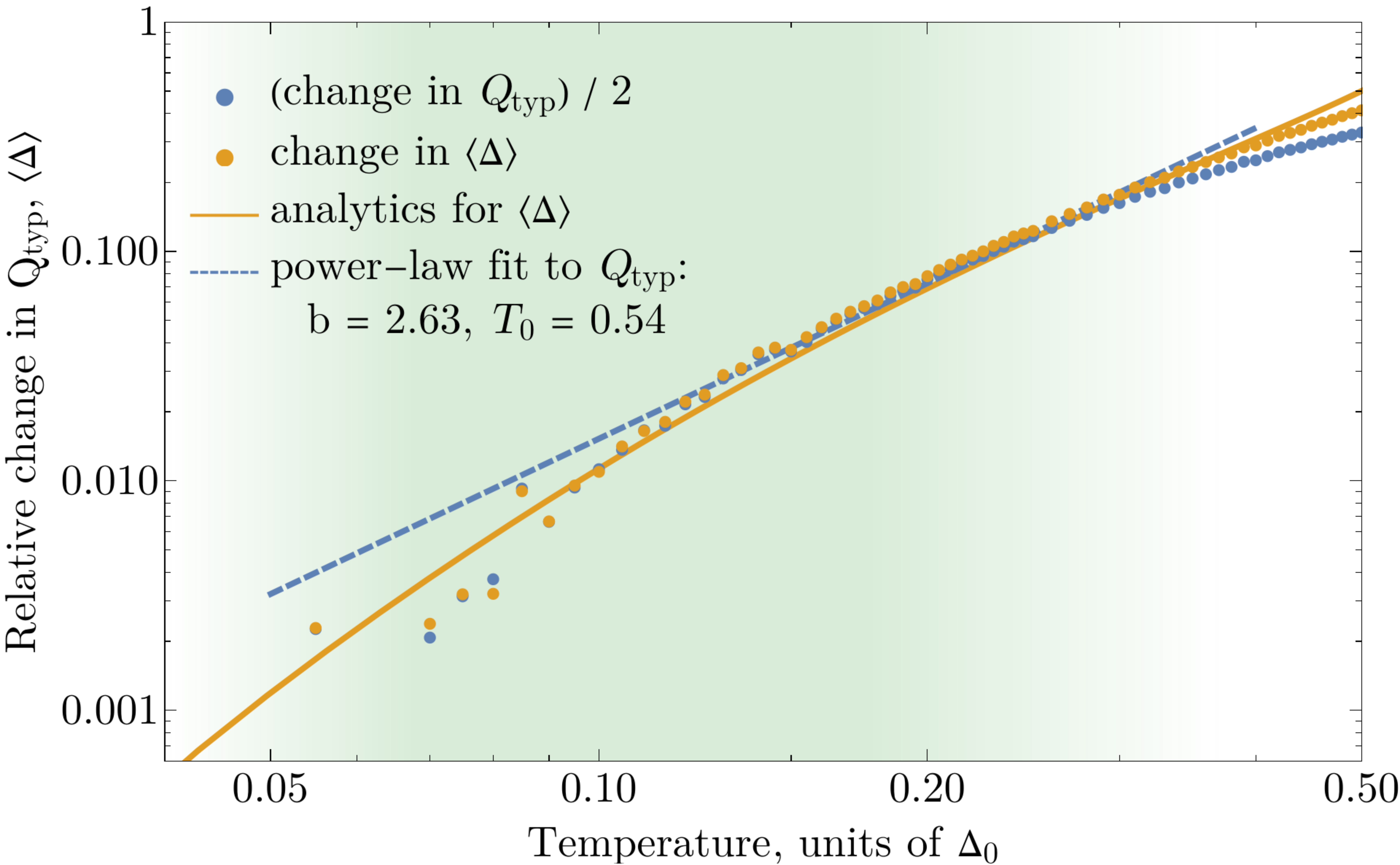
Figure 6: Low-temperature dependence of the relative changes in the typical local current response $\delta_{Q}=1-Q_{\text{typ}}\left(T\right)/Q_{\text{typ}}\left(T=0\right)$ and the mean order parameter $\delta_{\Delta}=1-\left\langle\Delta\right\rangle\left(T\right)/\left\langle\Delta\right\rangle\left(T=0\right)$ according to the numerical MPD (solid dots) and theoretical description given by Eqs. (48-49) (solid line) in logarithmic scale along both axes. The values of $\delta_{Q}$ are divided by two, which makes relation (34) apparent. The dashed line corresponds to the power-law fit $\left(T/T_{0}\right)^{b}$ of numerical data for $\delta_{Q}$ in the range $T\in\left[\lambda\left\langle\Delta\right\rangle,\lambda\left\langle\Delta\right\rangle+0.2\right]$, with $\left\langle\Delta\right\rangle=0.49\,\Delta_{0}$ (the values of the fitting curve are also divided by two). The parameters of the model are $K=20,\,\kappa=10$. The green region delineates the limits of applicability of the theoretical approach corresponding to $\lambda\left\langle\Delta\right\rangle\leq T\leq\left\langle\Delta\right\rangle/2$.

We also note that the proposed description naturally incorporates the small disorder limit $\kappa\ll 1$. In this case, the distribution of the order parameter is accurately described by a narrow Gaussian distribution, leading to a BCS-like behavior of the form $e^{-2\left\langle\Delta\right\rangle/T}$ for both $\delta Q_{\text{typ}}$ and $\delta\left\langle\Delta\right\rangle$, as demonstrated on 7. In terms of our analysis, this corresponds to replacing the $m$ function by a Gaussian one:

$$m\left(it\right)\approx-\left\langle h\right\rangle t-\frac{\pi\kappa\lambda}{4}t^{2},$$ (54)

which corresponds to small-$t$ expansion of the exact expression (37). This further reinforces the general conclusion: the nontrivial power-law-like behavior of physical quantities is the direct consequence of the nontrivial distribution of the order parameter $\Delta$. We also emphasize that the BCS-like result on 7 is obtained in the model with no quasi-particles (due to large pseudo-gap); as a result, the activation energy is equal to twice superconducting gap, instead of the gap itself.

One may wonder if some modified activation-type behavior could describe the data and our simulation results even at large $\kappa$. The corresponding analysis is presented in D. In particular, 11 shows that the activation-law fit $\delta\Theta(T)\sim\exp\left\{-T_{1}/T\right\}$ works in a limited range of temperature, and the latter shrinks as the dimensionless disorder strength $\kappa$ increases. However, for a larger value of the coordination number, $K=20$, we cannot numerically resolve the distinction between power-law and exponential fits, see 12.

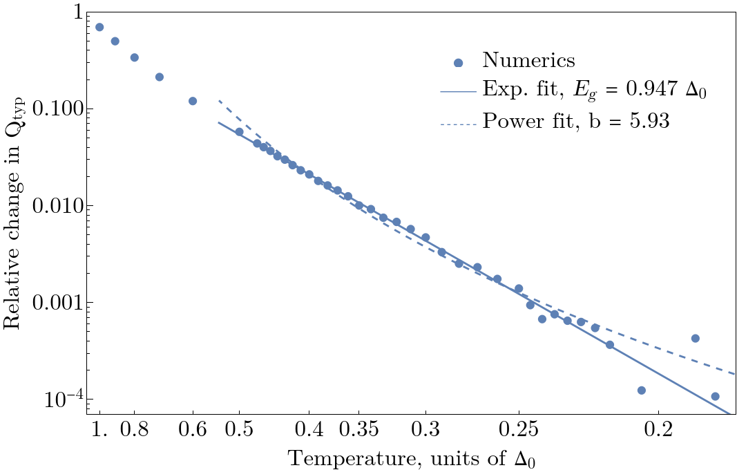
Figure 7: The temperature dependence of the relative change of typical local current response $1-Q_{\text{typ}}\left(T\right)/Q_{\text{typ}}\left(T=0\right)$ for $\kappa=0.25,\,\,K=10$ (small disorder). The temperature is measured in units of $\Delta_{0}$. The scale along the horizontal axis is reciprocal ($1/T$), and the scale of the vertical axis is logarithmic. The solid line corresponds to fit of the points with $T\leq 0.45\,\Delta_{0}$ with $A\exp\left\{-2E_{g}/T\right\}$, resulting in $A=2.41,\,\,E_{g}=0.947\,\Delta_{0}$, which is consistent with the standard BCS theory. Attempting to fit the same points with a power law $\left(T/T_{0}\right)^{b}$ results in $b\sim 5.9$ (shown with the dashed line).

V Discussion and Conclusions

We presented both experimental data and analytical theory of the low-temperature suppression of superfluid stiffness, $\delta\Theta(T)=\Theta(0)-\Theta(T)$, in strongly disordered pseudogapped superconductors.

The direct measurement of the superfluid stiffness at low temperatures $T\ll T_{c}$ in amorphous $\text{InO}_{x}$ films revealed (see Fig. 1 c) a strong deviation from the activation-like behavior expected within the semiclassical theory [19]. We observed instead a power-law

$$\delta\Theta(T)/\Theta(0)\sim\left(T/T_{0}\right)^{b},$$ (55)

with an exponent $b\sim 1.6$ that is weakly sensitive to the disorder strength and a characteristic scale $T_{0}$ that is roughly proportional to the superfluid stiffness at low temperatures, viz., $T_{0}\sim 5.5\,\Theta(0)$, see Fig. 2. A systematic departure from (55) towards higher values of $\delta\Theta$ is observed at higher temperatures ($T\apprge 0.2T_{c}\approx 0.5\,\text{K}$) for the less disordered films, and might be attributed to the conventional Mattis-Bardeen contribution due to quasiparticles.

To describe the experimental data, we developed an analytical approach based on a microscopic model of strongly disordered superconductor previously proposed in the literature [46, 33, 22]. The key ingredient of the model is the presence of a broad distribution of the local pairing amplitude $\Delta(\mathbf{r})\neq\text{const}$. The latter is known to exist [1] in a relatively wide range of normal-state resistances and was described theoretically in Ref. [22]. The qualitative behavior of the whole model is characterized primarily by the dimensionless disorder strength $\kappa$. In particular, an estimation for $\kappa$ can be extracted from the observed shape of the pairing amplitude distribution $P(\Delta)$ at large values [22]. The main challenge of the theoretical description is to connect theoretically computable distribution $P\left(\Delta\right)$ with physically observable quantities (e.g., the superfluid stiffness $\Theta$), as the latter can no longer be expressed via the pairing amplitude in a simple fashion.

By combining analytical and numerical methods, we have shown that this model also exhibits near-power-law suppression (55) of the superfluid stiffness with temperature (see 3), with disorder-dependent exponent $b\sim 1.6-3$ in the region of large disorder, $\kappa\gg 1$. In particular, the exponent $b$ decreases with disorder and may become less than 2, as shown on 4. The characteristic temperature $T_{0}$ in Eq. (55) is found to be of the order of the mean pairing amplitude $\left\langle\Delta\right\rangle$. The dependence (55) takes place in the temperature range $\lambda\left\langle\Delta\right\rangle\leq T\leq\left\langle\Delta\right\rangle/2$, and the temperature range itself reaches low temperatures $T\ll\left\langle\Delta\right\rangle$ due to the smallness of the dimensionless Cooper coupling constant $\lambda$. However, even within this temperature interval the power-law profile is only approximate, rendering the effective values of $b$ and $T_{0}$ temperature-dependent. In particular, 5 demonstrates that the "local" value of $b$ decrease with the growth of temperature. At very low temperatures $T\apprle\lambda\left\langle\Delta\right\rangle$, the value of $\delta\Theta$ is better described by an activation law $\delta\Theta/\Theta\sim\exp\left\{-2\lambda\left\langle\Delta\right\rangle/T\right\}$ with a diminished value of the gap in comparison to its semiclassical value. This behavior results in lower values of $\delta\Theta$ than those suggested by Eq. (55). At high temperatures $T\sim\Delta$, our theory is not applicable to the complete lack of quasiparticles within the proposed model.

However, even in the absence of the latter, we find within the same formalism for the case of small disorder $\kappa\ll 1$ the activation behavior $\delta\Theta/\Theta\sim\exp\left\{-2\left\langle\Delta\right\rangle/T\right\}$, but with twice the standard value of the gap, see 7. The effective gap is doubled since the energy $2\Delta$ corresponds in our case to a single excitation instead of two quasi-particles in the usual BCS theory.

As a result, one can claim qualitative agreement between theory and experiment, while a quantitative match is currently beyond reach due to numerous simplifications employed in the theoretical model. The quantitative result of our theory (summarized on 6) is only valid in the model (9) with weak statistical fluctuations of the magnitude of interaction matrix elements $J_{ij}$. As discussed in Ref. [22], strong fluctuations of the matrix elements render the low-value tail of the distribution of the order parameter even more pronounced and can thus increase the reported suppression of $\Theta$ as well as change the overall shape of the temperature dependence. As a result, the latter will still resemble a power-law, probably with a smaller exponent $b$, due to a substantial fraction of system sites with $\Delta_{i}<\left\langle\Delta\right\rangle$. An accurate description of the matrix element $J_{ij}$ and the resulting effects on the superfluid density and other physical observables are subjects of future work. We also emphasize that these unusual low-$T$ properties are predicted to exist even at relatively large $K\geq\lambda\exp(1/2\lambda)$, where the replica-symmetry-breaking theory of the SIT [34] is not yet relevant. An additional element missed in our simplified theory is the implication of the energy dependence of matrix elements $J_{ij}$, which is present due to Mott hybridization mechanism, as discussed in Ref. [33, Sec. 2.2.5]; this issue we also leave for future studies.

Among other things to be considered in the future is the issue of the relation between the macroscopic superfluid stiffness $\Theta$ and the local current response $Q^{\alpha\beta}\left(\omega;r,r^{\prime}\right)$ discussed in III.3. The approximate Eq. (24) is currently supported by certain preliminary simulations as well as similarity to the problem of the macroscopic response of disordered 2D media discussed in Ref. [39], while a qualitative solution to this problem is to be addressed in the near future. Importantly, the employed approximation does not give access to the superfluid stiffness itself, providing only its relative suppression with temperature $\delta\Theta/\Theta$. This difficulty can be traced down to the fact that kinetic quantities, such as $\Theta$, include information about the embedding of the model in real space. For instance, the semiclassical expression $\Theta\left(T=0\right)=\hbar\pi\Delta/(2e)^{2}R_{\square}$ valid for weak disorder contains this information via the normal-state resistivity per square $R_{\square},$ with the latter typically determined experimentally. However, sufficiently disordered a:InO films as well as the theoretical model used in the present paper demonstrate insulating behavior in the normal state [28], so experimentally measured $R_{\square}$ at $T>T_{c}$ might be delivered by a different mechanism than the one responsible for the formation of finite superfluid stiffness $\Theta$ for $T<T_{c}$, rendering $R_{\square}$ irrelevant for the value of $\Theta$. A consistent treatment of this issue would include a more elaborate account of the microscopic properties of the underlying single-particle Anderson localization problem, as the latter unavoidably enter the kinetic quantities.

Another important point worth examining more thoroughly is the validity of description of the local current response proposed in III.4. This comprises neglecting i) the quantum fluctuation and ii) the role of short loops that might be present in the interaction graph of the system. There does exist certain evidence in favor of the first approximation [34], but a more detailed analysis is required. The second of these approximations is at least partially controllable [35], but because our description involves dealing with extreme value statistics, small loops might be important for certain physical quantities. However, estimations of Ref. [22] indicate that finite concentration of short loops does not change the distribution of the order parameter at low temperature, leaving the effect on physical quantities for future studies.

On purely phenomenological grounds, the presence of nearly power-law behavior (55) indicates the existence of low-energy excitations with energies much below $\left\langle\Delta\right\rangle$. The nature of these excitations can be revealed by the analysis of dissipation properties of the same microwave resonances used to determine the spectrum of plasmon waves [28, 47]. We expect that the majority of these modes are localized at the scale of the typical interaction length between preformed Cooper pairs (up to few localization lengths). Therefore these modes may represent a specific kind of two level quantum systems (TLS). While those are usually related with atomic degrees of freedom in amorphous solids [48] or localized quasiparticles [49], in our case those TLS are formed by the coherent hopping of the Cooper pairs across several neighboring sites. An indication of the presence of TLS is the non-monotonic temperature dependence of the microwave resonance quality factor $Q(T)$, with a maximum at some nonzero temperature [28]. However, the observed data does not rule out the existence of additional mechanisms of dissipation at non-zero frequency. One such mechanism could be an analogue of the Debye relaxation recently discussed in relation with superconductors in the mixed state [50, 51].

Appendix A Electrodynamics of a disordered superconductor

In this Appendix, we formulate the low-frequency description of the electromagnetic response of a disordered superconductor, with the particular aim of deriving Eq. (20).

Consider the Fourier transform of the Maxwell equations for the electromagnetic potentials $\left(\varphi,\boldsymbol{A}\right)$ in the Coulomb gauge $\text{div}\boldsymbol{A}=0$:

$$\begin{cases}-\Delta\varphi=4\pi\rho/\varepsilon\left(\omega\right),\\ \left(-\Delta+\left(\frac{i\omega}{c}\right)^{2}\right)\boldsymbol{A}+\nabla\left(\frac{i\omega}{c}\varphi\right)=\frac{4\pi}{c}\boldsymbol{j},\\ \boldsymbol{E}=-\nabla\varphi-\frac{i\omega}{c}\boldsymbol{A}.\end{cases}$$ (56)

where $\varepsilon\left(\omega\right)$ is the dielectric permittivity due to the media surrounding the superconductor and the electrons deep within the Fermi surface (for simplicity, we neglect its spatial dependence, it can straightforwardly be restored). All fields here depend on the frequency $\omega$ and on the coordinate $\boldsymbol{r}$. The material response fields $\rho,\boldsymbol{j}$ are to be determined from

$$\begin{cases}j^{\alpha}\left(r\right)=\frac{c}{i\omega}\intop dr^{\prime}\,Q^{\alpha\beta}\left(\omega,r,r^{\prime}\right)\,E^{\beta}\left(r^{\prime}\right),\\ \rho\left(r\right)=-\frac{c}{i\omega}\intop dr^{\prime}\,R^{\beta}\left(\omega,r,r^{\prime}\right)E^{\beta}\left(r^{\prime}\right),\end{cases}$$ (57)

and are bound to satisfy the charge conservation law

$$i\omega\rho+\text{div}\boldsymbol{j}=0.$$ (58)

Here, the kernels $Q$ and $R$ are the material responses of the medium to the vector potential computed as direct variational derivatives:

$$Q^{\alpha\beta}\left(t-t^{\prime};r,r^{\prime}\right)=-\frac{\delta\left\langle j^{\alpha}\left(t,r\right)\right\rangle}{\delta A^{\beta}\left(r^{\prime},t^{\prime}\right)},$$

$$R^{\beta}\left(t-t^{\prime};r,r^{\prime}\right)=\frac{\delta\left\langle\rho\left(t,r\right)\right\rangle}{\delta A^{\beta}\left(r^{\prime},t^{\prime}\right)}.$$ (59)

As per usual, the system (56-58) is over-complete because the second equation in Eq. (57) describing the charge density response is actually satisfied automatically by the true configuration of the electromagnetic fields due to the charge conservation law, Eq. (58), so we can discard this equation. We can then exclude the charge variable with the help of Eq. 56 and obtain

$$\begin{cases}\text{div}\boldsymbol{j}=i\omega\,\frac{\Delta\varphi}{4\pi\varepsilon\left(\omega\right)}\\ \left(-\Delta+\left(\frac{i\omega}{c}\right)^{2}\right)\boldsymbol{A}+\nabla\left(\frac{i\omega}{c}\varphi\right)=\frac{4\pi}{c}\boldsymbol{j},\\ \text{div}\boldsymbol{A}=0,\\ \boldsymbol{E}=-\nabla\varphi-\frac{i\omega}{c}\boldsymbol{A},\\ j^{\alpha}\left(r\right)=\frac{c}{i\omega}\intop dr^{\prime}\,Q^{\alpha\beta}\left(\omega,r,r^{\prime}\right)E^{\beta}\left(r^{\prime}\right).\end{cases}$$ (60)

We now want to calculate the superconducting response to a given external electromagnetic field $E_{\text{ext}}\left(r,t\right)$, which is created by currents other than those in the material in question. Certainly, this external field automatically satisfies the first four relations in system (60), but with the current density $\boldsymbol{j}$ produced by some external sources (whose currents are obviously unaltered by the response of the medium). Therefore, to analyze the response of the target medium we have to the substitute the full electric field $\boldsymbol{E}_{\text{full}}=\boldsymbol{E}+\boldsymbol{E}_{\text{ext}}$ in the last expression describing the current response of the medium. In this way, the Eqs. (60) are rendered inhomogeneous, so the response problem is well-formulated.

The main difference of the resulting system of equations (60) with the standard semiclassical description is that due to the inhomogeneity of the superconducting state the current conservation law is not satisfied “automatically” by an appropriate choice of gauge. Instead, the system adjusts the values of microscopic currents and induced electromagnetic field in order to satisfy the charge conservation, making the resulting value of the macroscopic response much more complicated than simply the mean value of the miscroscopic response. In this way, the problem is similar to the one of the macroscopic conductance of a disordered media, where the potential distribution is determined from the charge conservation (or, equivalently, the Kirchhoff’s rule for a discrete system).

We are interested in the low-frequency limit of the system (60). Because the system is superconducting, the zero-frequency response function $Q^{\alpha\beta}\left(\omega=0,r,r^{\prime}\right)$ does not vanish. Eqs. 60 then suggest the following substitution to reproduce the correct low-frequency behavior of the response:

$$\boldsymbol{j}=\frac{\boldsymbol{u}}{i\omega},\,\,\,\boldsymbol{A}=-\frac{c}{i\omega}\boldsymbol{\mathcal{E}}$$ (61)

which then leads to the following equivalent system:

$$\begin{cases}\text{div}\boldsymbol{u}=\left(i\omega\right)^{2}\,\frac{\Delta\varphi}{4\pi\varepsilon\left(\omega\right)},\\ \left(-\Delta+\left(\frac{i\omega}{c}\right)^{2}\right)\left(-c\boldsymbol{\mathcal{E}}\right)+\nabla\left(\frac{\left(i\omega\right)^{2}}{c}\varphi\right)=\frac{4\pi}{c}\boldsymbol{u},\\ \text{div}\boldsymbol{\mathcal{E}}=0,\\ \boldsymbol{E}=-\nabla\varphi_{r}+\boldsymbol{\mathcal{E}},\\ u^{\alpha}\left(r\right)=c\intop dr^{\prime}\,Q^{\alpha\beta}\left(\omega;r,r^{\prime}\right)\,E_{\text{full}}^{\beta}\left(r^{\prime}\right).\end{cases}$$ (62)

One can then take the zero-frequency limit of these equations by simply putting $\omega=0$, which renders

$$\begin{cases}\text{div}\boldsymbol{u}=0,\\ \Delta\boldsymbol{\mathcal{E}}=\frac{4\pi}{c^{2}}\boldsymbol{u},\\ \text{div}\boldsymbol{\mathcal{E}}=0,\\ \boldsymbol{E}=-\nabla\varphi_{r}+\boldsymbol{\mathcal{E}},\\ u^{\alpha}\left(r\right)=c\intop dr^{\prime}\,Q^{\alpha\beta}\left(0;r,r^{\prime}\right)\,E_{\text{full}}^{\beta}\left(r^{\prime}\right).\end{cases}$$ (63)

As we can see, even in the limit of vanishing frequency, the medium generally responses both by electric and magnetic fields, as $\text{rot}\boldsymbol{E}=\text{rot}\boldsymbol{\mathcal{E}}\neq\boldsymbol{0}$. However, there’s a natural division of scales in this equations, which allows one to simplify the system significantly as far as the value of the superfluid stiffness is concerned. Let’s decompose all fields into a sum of fast and slow components, with the distinction made along the scale $l_{\text{m}}$ at which one can consider the superfluid stiffness as a self-averaging quantity. The order of $l_{\text{m}}$ can roughly be estimated by the size of the tree-like structure of the underlying interaction graph (see III.1 of the main text), so $l_{\text{m}}\sim C\xi_{\text{loc}}$, where $C$ is a number of order 2. In this case, all equations except the last in system (63) independently describe slow and fast components, while the last equation in system (63) mixes both slow and fast components of the field $\boldsymbol{E}$ due to small spatial scale of the change in the $Q$ kernel. However, from the second equation in system (63) the fast component of $\boldsymbol{\mathcal{E}}$ can be estimated as

$$\boldsymbol{\mathcal{E}}^{\left(\text{fast}\right)}\sim\frac{4\pi}{c^{2}}l_{\text{m}}^{2}\boldsymbol{u}\sim\frac{4\pi}{c}l_{\text{m}}^{2}\rho_{S}\boldsymbol{E}\sim\frac{l_{\text{m}}^{2}}{\lambda_{L}^{2}}\boldsymbol{E},$$ (64)

where $\lambda_{L}=\sqrt{c^{2}/4\pi\rho_{S}}$ is the London penetration depth. Because we expect $\lambda_{L}\gg l_{m}$, this contribution to the electric field is small, so we can neglect it and obtain

$$\begin{cases}\text{div}\boldsymbol{u}=0,\\ \boldsymbol{E}=-\nabla\varphi,\\ u^{\alpha}\left(r\right)=c\intop dr^{\prime}\,Q^{\alpha\beta}\left(0;r,r^{\prime}\right)E_{\text{full}}^{\beta}\left(r^{\prime}\right),\end{cases}$$ (65)

which is equivalent to Eq. (20) presented in the main text. Note that this only works for the response at small scales, while at large scales one still has to solve the exact system (63). However, because we expect that the superfluid responses averages over scales $l_{\text{m}}$, one can replace the last equation with a simple London-type relation at large scales:

$$\begin{cases}\text{div}\boldsymbol{u}=0,\\ \Delta\boldsymbol{\mathcal{E}}=\frac{4\pi}{c^{2}}\boldsymbol{u},\\ \text{div}\boldsymbol{\mathcal{E}}=0,\\ \boldsymbol{E}=-\nabla\varphi+\boldsymbol{\mathcal{E}},\\ u^{\alpha}\left(r\right)=\rho_{S}E_{\text{full}}^{\beta}\left(r\right),\end{cases}$$ (66)

which can be cast in the form of the standard London equations because for $\rho_{S}=\text{const}$ the solution for $\varphi$ is trivial, viz. $\varphi\left(r\right)=0$:

$$\begin{cases}\text{div}\boldsymbol{j}=0,\\ -\Delta\boldsymbol{A}=\frac{4\pi}{c}\boldsymbol{j},\\ \text{div}\boldsymbol{A}=0,\\ \boldsymbol{j}=-\frac{1}{c}\rho_{S}\boldsymbol{A}_{\text{full}}.\end{cases}$$ (67)

Another case where the approximate Eqs. (65) are applicable is that of a response of a thin film, for which the magnetic part of the response is small regardless of the scale, so one neglect it and put $\boldsymbol{\mathcal{E}}=\boldsymbol{0}$.

As a result, the system (62) accurately describes the full electromagnetic response of a disordered superconductor, with the system (63) being the corresponding low-frequency limit. This includes both the microscopic effects arising from strongly inhomogeneous superconducting state and the macroscopic effects such as the Meissner effect. At the same time, the division of scales or smallness of the absolute value of the currents in the material (such as in case of a thin film) allow one to determine the superfluid density of such a superconductor by using the potential approximation, Eqs. (65), i.e., neglecting the magnetic part of the response.

Appendix B Spatial structure of the current response to a potential electric field

In this Appendix, we analyze the spatial structure of the low-frequency current response to a potential electric field. In particular, we derive Eq. (21) used to determine the superfluid density in the system via the characteristics of the problem on a graph. We start from verifying the discrete current conservation identity. According to Eq. (11), the charge conservation condition $\text{div}\boldsymbol{j}=0$ corresponds to

$$0=\frac{1}{2}\sum_{e}\text{div}\boldsymbol{D}_{e}\left(\boldsymbol{r}\right)\,I_{e},$$ (68)

where $I_{e}$ is the current along directed edge $e$. Due to identity (16), this equation reduces to

$$0=\sum_{i}\left|\psi_{i}\left(\boldsymbol{r}\right)\right|^{2}\,\sum_{j\in\partial i}I_{i\rightarrow j},$$ (69)

where we have used current anti-symmetry $I_{i\rightarrow j}=-I_{j\rightarrow i}$. This should be true for any point $\boldsymbol{r}$, which is only possible if the coefficient in front of each $\left|\psi_{i}\left(\boldsymbol{r}\right)\right|^{2}$ vanishes, rendering the discrete charge conservation, Eq. (21).

We should now establish the connection between the current response function in real space and that on the graph. The vector potential is coupled to the system as $H_{\text{EM}}=-\frac{1}{c}\intop d\boldsymbol{r}^{\prime}\,\left(\boldsymbol{j}\left(\boldsymbol{r}\right),\boldsymbol{A}\left(\boldsymbol{r}\right)\right)$, which, together with Eq. (11), implies that the response of $I_{e}\left(t\right)$ to $\boldsymbol{A}\left(t,\boldsymbol{r}\right)$ reads

$$I_{e}\left(t\right)=-\frac{1}{2}\sum_{e^{\prime}}\,\intop dt^{\prime}\,Q_{ee^{\prime}}\left(t,t^{\prime}\right)\,A_{e^{\prime}}\left(t^{\prime}\right),$$ (70)

where the discrete edge potential $A_{e^{\prime}}$ is given by (15), and $Q_{ee^{\prime}}\left(t,t^{\prime}\right)$ is the nonlocal current response on the graph, including the diamagnetic term due to the explicit dependence of the current operator on the vector potential, Eq (12).

According to Eq. (20), we are interested in the current response to a potential vector field $\boldsymbol{A}=c/i\omega\,\nabla\phi$, for which Eqs. (15) and (16) allow to express the corresponding discrete edge potential as

$$A_{e}=\frac{c}{i\omega}\,\frac{\phi_{\text{end}\left(e\right)}-\phi_{\text{beg}\left(e\right)}}{2},$$ (71)

where for a directed edge $e=i\rightarrow j$ we denoted $\text{end}\left(e\right)=j$ and $\text{beg}\left(e\right)=i$, and the discrete field $\phi_{i}$ is defined according to Eq. (23) of the main text. This expression can further be reformulated in terms of the edge potential induced by a scalar potential applied to a given site $j$:

$$A_{e}=\sum_{j}A_{e}^{\left(j\right)},\,\,\,A_{e}^{\left(j\right)}=\begin{cases}\frac{c}{i\omega}\frac{\phi_{j}}{2},&\text{end}\left(e\right)=j,\\ -\frac{c}{i\omega}\frac{\phi_{j}}{2},&\text{beg}\left(e\right)=j,\\ 0,&\text{otherwise}.\end{cases}$$ (72)

Our next step will be to compute the response of the current along a given edge $e$ to the edge potential of the form (72) within the AQBP scheme described in III.4 of the main text. Together with Eqs. (70) and (11), this allows us to calculate the density current $\boldsymbol{j}\left(\boldsymbol{r}\right)$ in the response to the potential field at low frequencies and eventually derive Eq. (21) the main text.

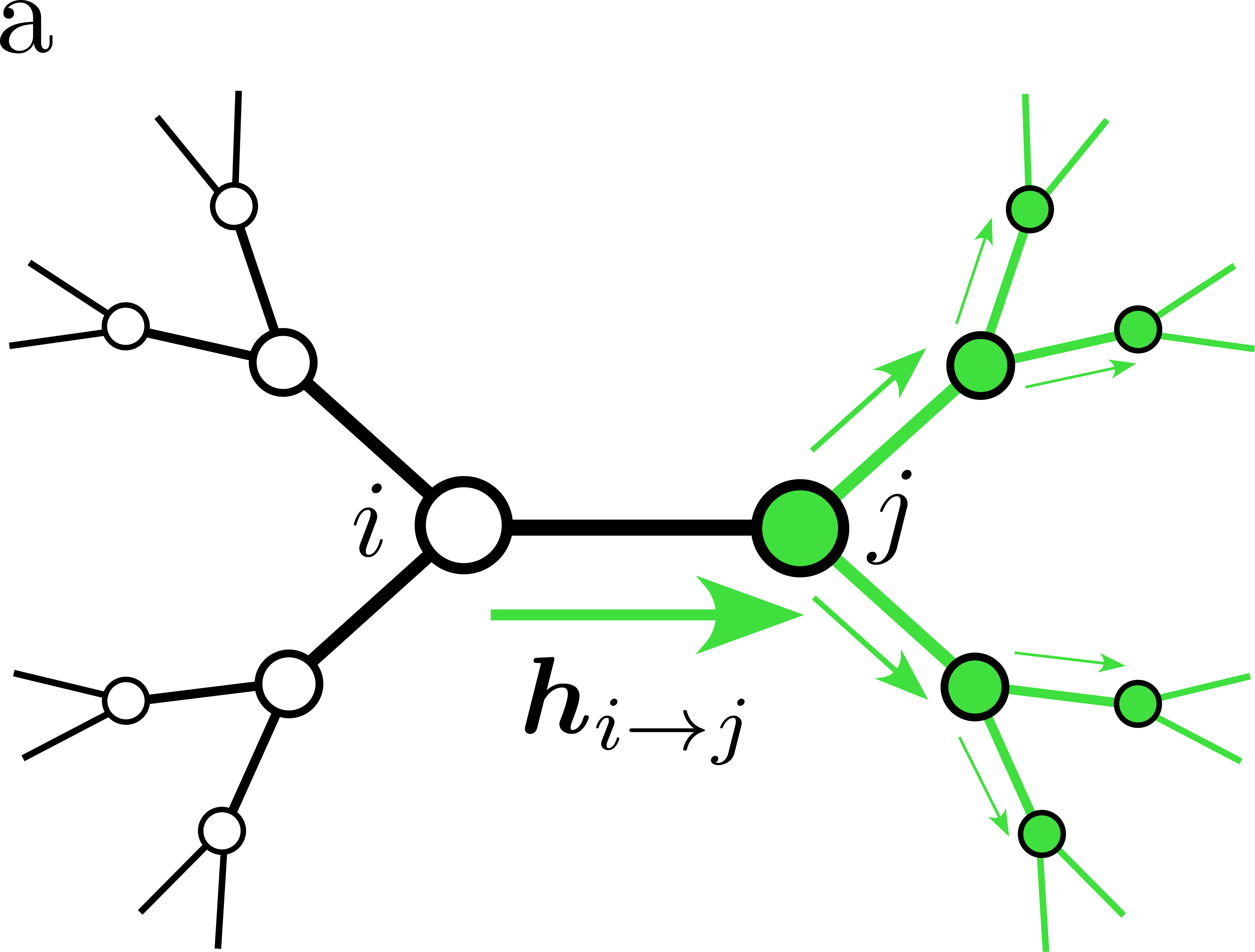
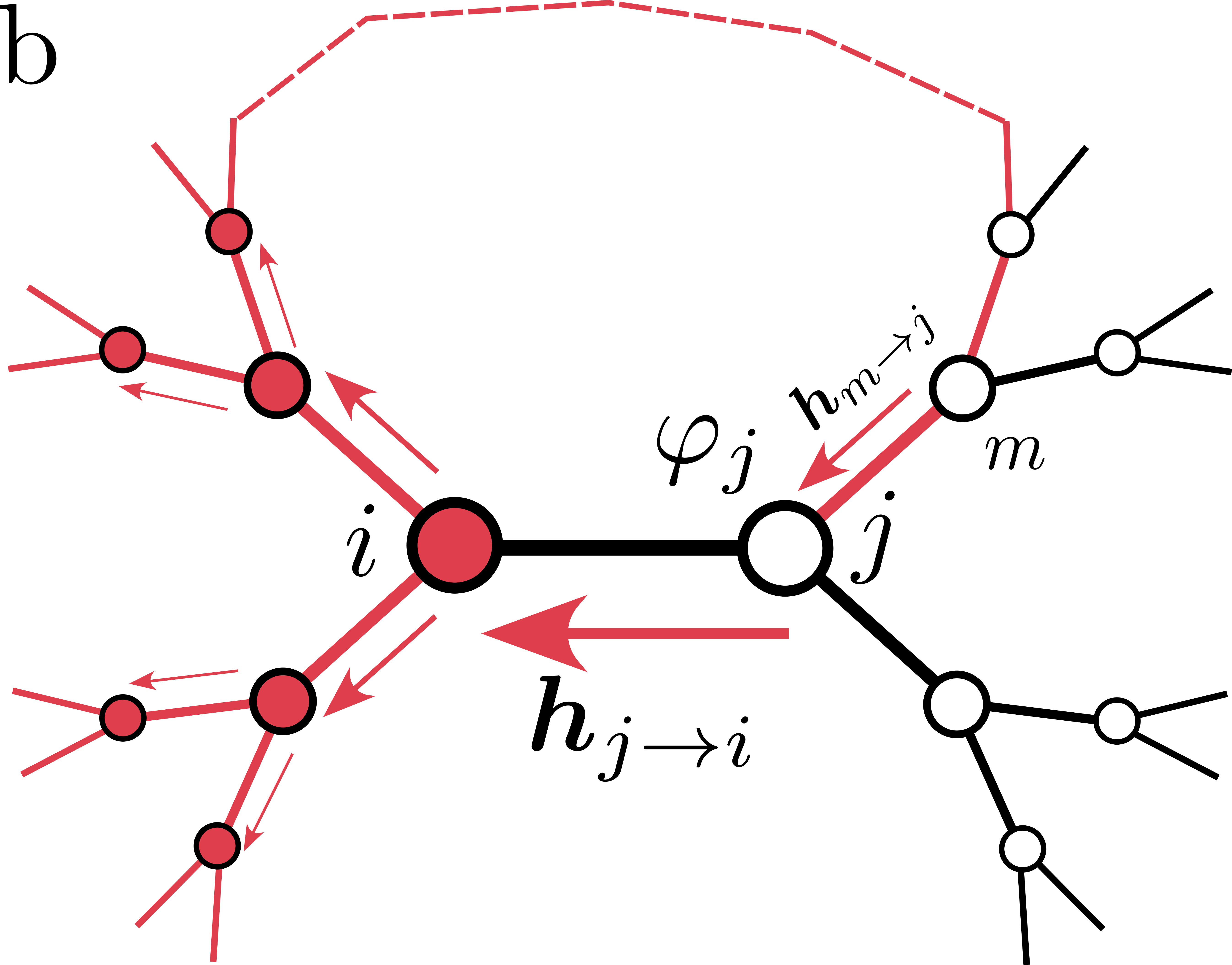
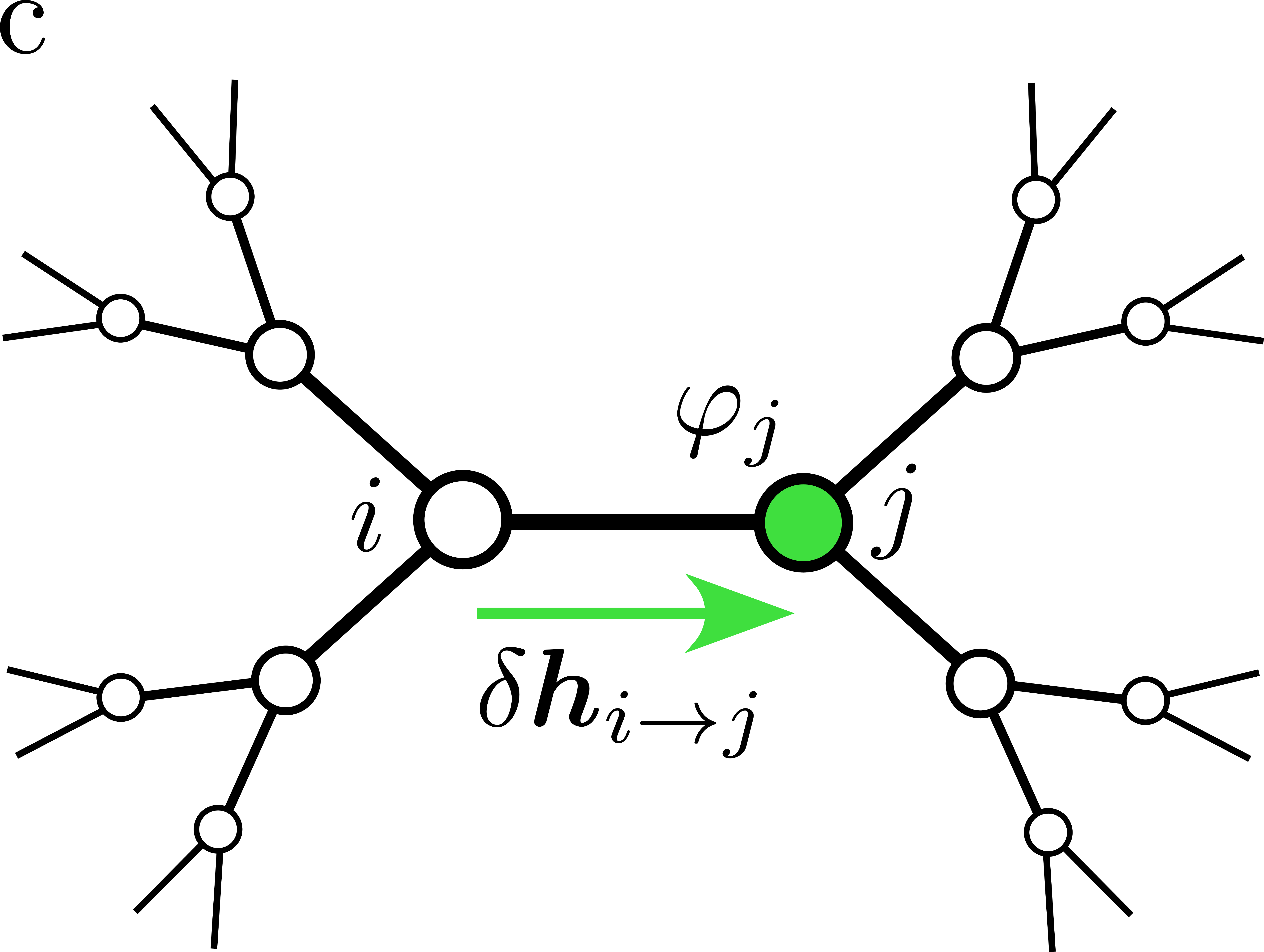
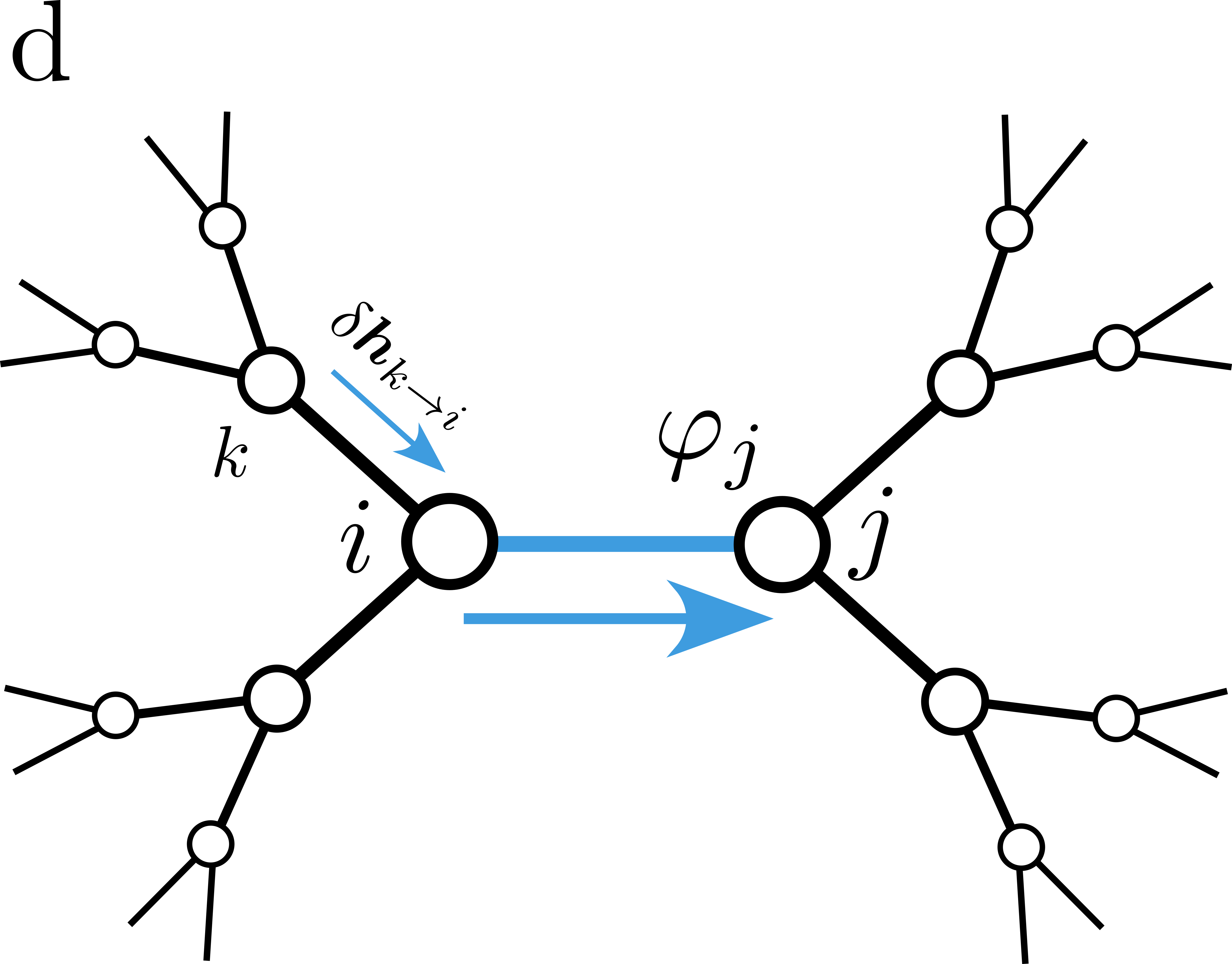
Figure 8: Visualization of the structure of dependencies in the self-consistency equation (74) on a locally tree-like graph with coordination number $Z=3$. a) the value of the $h$ associated with a given directed edge is influenced by the branch originating from the end vertex of this directed edge (colored in green), and only the values of $h$ along the edges oriented in the same direction contribute to the equation. b) Due to the presence of a large loop (red dashed line), the other branch of the graph also has some influence over the value of $h$, but according to Eq. (74), each edge in this loop contributes with an additional factor of $JP\sim 1/Z$ to the magnitude of this influence. As a result, the change of $h$ practically vanishes for all edges pointing away from the source site $j$. c) The change of $h$ on the edge ending at the source site $j$ is thus only sensitive to the source term itself d) The change of $h$ on the edge at distance greater than 1 away from the source site $j$ is sensitive only to the change of $h$ on the edge that precedes it on the path to the source.

The first step is to figure out the way to calculate the non-local response, by which we refer to the case when the edge $e$ in Eq. (70) does not belong the to the nearest neighborhood of site $j$ from Eq. (72). Within the AQBP scheme, any change in the operator on edge $e$ by a perturbation on a different edge $e^{\prime}\neq\pm e$ is produced by the response of the order parameter $\delta h_{e}$, so one has

$$Q_{ee^{\prime}}\left(t,t^{\prime}\right)=-\intop dt^{\prime\prime}\,\left[\frac{\delta\left\langle I_{e}\left(t\right)\right\rangle}{\delta\boldsymbol{h}_{e}\left(t^{\prime\prime}\right)}\cdot\frac{\delta\left\langle\boldsymbol{h}_{e}\left(t^{\prime\prime}\right)\right\rangle}{\delta A_{e^{\prime}}\left(t^{\prime}\right)}+\frac{\delta\left\langle I_{e}\left(t\right)\right\rangle}{\delta\boldsymbol{h}_{-e}\left(t^{\prime\prime}\right)}\cdot\frac{\delta\left\langle\boldsymbol{h}_{-e}\left(t^{\prime\prime}\right)\right\rangle}{\delta A_{e^{\prime}}\left(t^{\prime}\right)}\right],$$ (73)

where the two terms in the sum correspond to contribution from the two directions of the target edge. The change of the order parameter is, in turn, described by the time-dependent generalization of the self-consistency equation (26) of the main text:

$$\delta\boldsymbol{h}_{k\rightarrow i}\left(t\right)=\sum_{j\in\partial i\backslash\left\{k\right\}}J_{ij}\left[\intop dt\hat{P}_{i\rightarrow j}\left(t,t^{\prime}\right)\delta\boldsymbol{h}_{i\rightarrow j}\left(t^{\prime}\right)+\frac{2e}{c}A_{i\rightarrow j}\left(t\right)\left\langle 2S^{x}\right\rangle_{i\rightarrow j}\boldsymbol{e}_{y}\right],$$ (74)

where $\boldsymbol{e}_{y}$ is the unit vector along $y$ direction, $\left\langle 2S^{x}\right\rangle_{i\rightarrow j}$ is the static spin average given by Eq. (28) of the main text, and $P_{i\rightarrow j}^{\alpha\beta}\left(t,t^{\prime}\right)=\left\langle\left\langle 2S^{\alpha}\left(t\right)2S^{\beta}\left(t^{\prime}\right)\right\rangle\right\rangle$ is the polarization operator of a single spin with the Hamiltonian given by Eq. (27), whose Fourier transform reads

$$\hat{P}_{i\rightarrow j}\left(\omega\right)=\frac{\tanh\beta B_{i\rightarrow j}}{B_{i\rightarrow j}\left(B_{i\rightarrow j}^{2}-\omega^{2}/4\right)}\begin{pmatrix}\xi_{j}^{2}&\frac{i\omega\xi_{j}}{2}\\ -\frac{i\omega\xi_{j}}{2}&B_{i\rightarrow j}^{2}\end{pmatrix},$$ (75)

with $B_{i\rightarrow j}=\sqrt{\xi_{j}^{2}+h_{i\rightarrow j}^{2}}$, and $\omega$ shifted by $+i0$ to restore the retarded structure of the response. In Eqs. (74-75) we have set the direction of the unperturbed order parameter $h$ along the $x$ axis, analogous to the real order parameter configuration in conventional superconductors.

The first important thing to note about Eq. (74) for the edge potential $A_{e}^{\left(j\right)}$ given by Eq. (72) is that due to the locally tree-like structure of the graph and directed nature of this equation, $\delta\boldsymbol{h}_{e}=\boldsymbol{0}$ for all edges that are directed away from the site $j$ where the potential is applied. For instance, one has $\delta\boldsymbol{h}_{j\rightarrow i}=0$ for any neighboring site $i\in\partial j$, whereas $\delta\boldsymbol{h}_{i\rightarrow j}\neq\boldsymbol{0}$, as we will see later. This is apparent from the fact that for all edges $e$ directed away from site $j$, the homogeneous part of Eq. (74) contains only edges $e^{\prime}$ that originate from $\text{end}\left(e\right)$ and point away from $j$ as well, as explained on 8. The same figure also illustrates that the actual value of $\delta\boldsymbol{h}_{j\rightarrow i}$ in the system that contains loops of length at least $l$ can be estimated as $\delta h_{j\rightarrow i}\sim\left(JP\right)^{l/2}\delta h_{m\rightarrow j}\sim\left(1/Z\right)^{l/2}\delta h_{i\rightarrow j}$ because each additional edge traversed from the source of the perturbation to the target edge brings in additional power of $J\cdot P\sim\frac{1}{Z}$, i.e. it is indeed negligible.

Upon application of the edge potential of the form (72), $\delta\boldsymbol{h}_{i\rightarrow j}$ for any $i\in\partial j$ is described only by the source term of Eq. (74) and reads

$$\delta\boldsymbol{h}_{i\rightarrow j}=-\frac{2e}{i\omega}\sum_{s\in\partial j\backslash\left\{i\right\}}J_{js}\left\langle 2S^{x}\right\rangle_{j\rightarrow s}\,\frac{\phi_{j}}{2}\,\boldsymbol{e}_{y}.$$ (76)

We then immediately recognize the r.h.s of the static self-consistency equation (26) for $h_{i\rightarrow j}$, which leads to

$$\delta\boldsymbol{h}_{i\rightarrow j}=-\frac{2e}{i\omega}h_{i\rightarrow j}\frac{\phi_{j}}{2}\boldsymbol{e}_{y},$$ (77)

i.e. the time-dependent change $\boldsymbol{h}_{i\rightarrow j}$ of the order parameter for edges pointing at $j$ is transverse to the direction of the order parameter itself and directly proportional to the external field $\varphi_{j}$. This result is otherwise expected from the gauge invariance: one can move the potential from site $j$ to all sites of the system that are contained in branch rooted at $i$ by a time-depend gauge transform. Because there’s no direct response of $\boldsymbol{h}_{i\rightarrow j}$ to this new field due to the tree-like structure, as described above, the only thing that remains is the gauge change of $\boldsymbol{h}_{i\rightarrow j}$, which is given exactly by Eq. (77).

Consider now an edge $e=k\rightarrow i$ that is within distance 2 from site $j$, i.e. $\text{end}\left(e\right)\in\partial j$ but $\text{beg}\left(e\right)\neq j$ (see also 8). This time around, both terms in Eq. (74) contribute to the result, but the sum contains only one term corresponding to edge $i\rightarrow j$ that connects the target edge $e$ to the source site $j$:

$$\delta\boldsymbol{h}_{k\rightarrow i} =J_{ij}\left[\hat{P}_{i\rightarrow j}\left(\omega\right)\delta\boldsymbol{h}_{i\rightarrow j}+\frac{2e}{c}A_{i\rightarrow j}\left\langle 2S^{x}\right\rangle_{i\rightarrow j}\boldsymbol{e}_{y}\right]$$

$$=\frac{2e}{i\omega}J_{ij}\left[-h_{i\rightarrow j}\hat{P}_{i\rightarrow j}\left(\omega\right)\boldsymbol{e}_{y}+\left\langle 2S^{x}\right\rangle_{i\rightarrow j}\boldsymbol{e}_{y}\right]\frac{\phi_{j}}{2},$$ (78)

where we have used the Fourier representation of Eq. (74). Remarkably, in the $\omega\rightarrow 0$ limit, we observe from Eq. (75) that

$$h_{i\rightarrow j}\hat{P}_{i\rightarrow j}\left(0\right)\boldsymbol{e}_{y}\equiv\left\langle 2S^{x}\right\rangle_{i\rightarrow j}\boldsymbol{e}_{y},$$ (79)

so at zero frequency we arrive at

$$\delta\boldsymbol{h}_{k\rightarrow i}\left(\omega=0\right)=0.$$ (80)

Moreover, due to the fact that Eq. (74) contains only the first term for any edge that is not in the nearest neighborhood of site $j$, we arrive to

$$\delta\boldsymbol{h}_{e}\left(\omega=0\right)=0,$$ (81)

for any edge $e$ that is not in the nearest neighborhood of site $j$. This and Eq. (73) finally implies that in response to a potential on site $j$ the current is induced only along edges that are adjacent to $j$.

Finally, let’s compute the current response directly along the adjacent edge, i.e $e=i\rightarrow j$ for some $i\in\partial j$. This time round, the response of $I_{e}$ to the edge potential (72) contains both the nonlocal term from the edge potential on adjacent edges as well as the explicit current response to the vector potential on the same edge:

$$I_{e}=\intop dt^{\prime}\,\left[-Q_{ee}\left(t,t^{\prime}\right)\,A_{e}^{\left(j\right)}\left(t^{\prime}\right)+\intop dt^{\prime\prime}\,\,\frac{\delta\left\langle I_{e}\left(t\right)\right\rangle}{\delta\boldsymbol{h}_{e}\left(t^{\prime\prime}\right)}\cdot\sum_{e^{\prime}\neq-e:\text{beg}\left(e^{\prime}\right)=j}\frac{\delta\left\langle\boldsymbol{h}_{e}\left(t^{\prime\prime}\right)\right\rangle}{\delta A_{e^{\prime}}\left(t^{\prime}\right)}\,A_{e^{\prime}}^{\left(j\right)}\left(t^{\prime}\right)\right].$$ (82)

We now have to compute the current response to a change of the order parameter along the same edge. The current itself is described by the time-dependent version of the two-spin Hamiltonian (30), with one of the two $h$ fields now being the function of time. We first note that the current response to the change of the longitudinal component of the $\delta\boldsymbol{h}\propto\boldsymbol{e}_{x}$ field vanishes due to the symmetry of the two-spin Hamiltonian. Indeed, consider the transformation $S^{x}\mapsto-S^{x}$, $S^{y}\mapsto-S^{y}$ followed by $h^{x}\left(t\right)\mapsto-h^{x}\left(t\right)$, with both transformations applied to both sites. In the absence of the transverse field $h^{y}$, this transformation leaves both the two-spin Hamiltonian and the current intact, so we conclude that

$$\frac{\delta\left\langle I_{e}\left(t\right)\right\rangle}{\delta h_{e}^{x}\left(t^{\prime\prime}\right)}\equiv-\frac{\delta\left\langle I_{e}\left(t\right)\right\rangle}{\delta h_{e}^{x}\left(t^{\prime\prime}\right)}=0.$$ (83)

The response to the transverse component $\delta\boldsymbol{h}\propto\boldsymbol{e}_{y}$ can be calculated by performing a gauge transform on the corresponding spin, which delivers the following identity:

$$\frac{\delta\left\langle I_{e}\left(t\right)\right\rangle}{\delta\boldsymbol{h}_{e}\left(t^{\prime\prime}\right)}=\frac{1}{\left(2e\right)/c}\frac{Q_{ee}\left(t,t^{\prime}\right)}{h_{e}}\boldsymbol{e}_{y}^{T},$$ (84)

This and Eq. (82) the renders the following identity for the value of the response to the potential field at the adjacent edge:

$$I_{e}=-\frac{1}{i\omega}\,cQ_{ee}\left(\omega\right)\,\phi_{j}.$$ (85)

According to Eqs. (70)-(72), to compute the current response from arbitrary configuration of the scalar potential, one should sum the responses over all sites $j$, while taking into account the anti-symmetry property $I_{j\rightarrow i}=-I_{i\rightarrow j}$. This finally renders for low frequencies

$$I_{i\rightarrow j}=-\frac{1}{i\omega}\,cQ_{ee}\left(0\right)\,\left(\phi_{j}-\phi_{i}\right),$$ (86)

where we neglected the frequency dependence of the $Q$ kernel. As a result, the current response to a potential field at zero frequency is present only along the edges adjacent to the site were the potential is applied, and the magnitude of this response coincides with the one calculated from the direct effect of the applied potential on this adjacent edge. Together with Eq. (11) this yields Eq. (21) of the main text.

Appendix C Verification of Dykhne’s law for a discrete system on a locally tree-like graph

The set of numerical experiments presented below demonstrates the approximate validity of the relation (24) in the following sense: the macroscopic response $\rho_{S}$ and the typical local response $Q_{\text{typ}}$ obey this relation as disorder strength $\kappa$ is varied within a fixed topology of the graph.

C.0.1 Generating the interaction graph.

For a given length $L$ and width $w$, $N\gg 1$ points were spread universally over a rectangle of size $L\times w$, with $L\gg w$. For each point, $Z$ neighbors were selected in the neighborhood of radius $\xi\ll L,w$ (periodic boundary conditions along the $w$ directions where used). To ensure the locally tree-like structure, the condition $Z\ll n\xi^{D}$ was also ensured (here $D=2$ is the dimensionality of the problem, and $n=N/Lw$ is the concentration). In case the condition of exactly $Z$ neighbors could not be satisfied for all $N$ sites, the number of such sites was controlled to be negligible (to maintain the average number of neighbors close enough to $Z$). In this way, the instance of a locally-tree like graph described in III.1 of the main text was obtained.

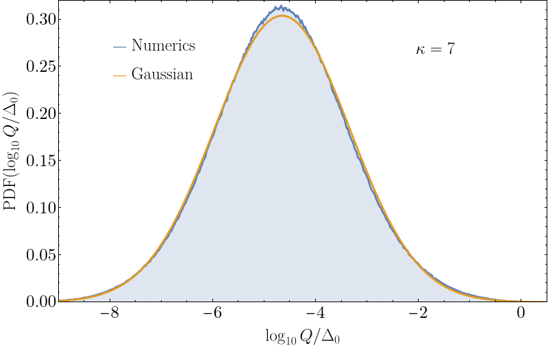
Figure 9: The distribution of the decimal logarithm of the current response functions, as found from the Eq. (29) of the main text. The parameters of the model are $T=0$, $\kappa=7,$ $\lambda=0.165$, $Z=6$. The orange curve corresponds to the Gaussian distribution with the parameters inferred from actual distribution: $\left\langle\log_{10}Q\right\rangle=-4.66$ and $\sqrt{\left\langle\left(\log_{10}Q\right)^{2}\right\rangle-\left\langle\log_{10}Q\right\rangle^{2}}=1.31$.

C.0.2 Determining the macroscopic response in a given disorder realization.

The next step was to determine the configuration of the order parameter according to Eq. (26) and calculate the local edge responses according to Eq. (29). Note that this procedure keeps track of the configuration of the $h$ fields and $Q$ values in a given disorder realization, in contrast to the MPD described in III.5 of the main text that addresses only the distribution of those quantities. 9 shows the distribution of the local responses $Q_{ij}$ in a typical disorder realization.

Eqs. (21) (discarding the irrelevant $-c/i\omega$ factor in front of the current) were then solved numerically with the following boundary conditions: $\varphi_{i}=0$ for a strip of size $d\times w$ with $n^{-1/D}\ll d\ll L$ near the one of the system’s boundaries, and $\varphi_{i}=\varphi_{0}$ for a strip of the same size situated at the other boundary, thus arranging the geometry of the two-contact measurement. The resulting distribution of the potential was used to determine the distribution of current $I_{i\rightarrow j}$. The total current $I_{\text{total}}$ was then calculated as a sum of the currents along all edges that connected a site inside the strip of fixed potential with a site outside of this strip. The resulting value of the superfluid density $\rho_{S}=\varphi_{0}w/I_{\text{total}}L$ was then recorded for a given disorder realization.

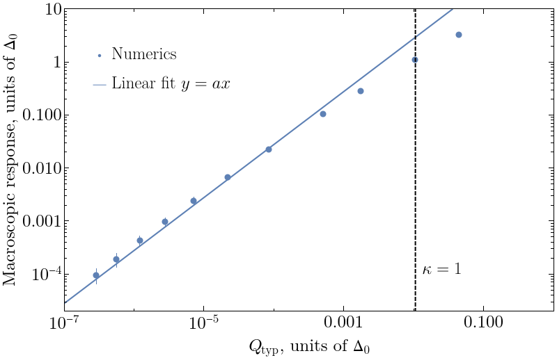
Figure 10: Set of points corresponding to pairs $\left(Q_{\text{typ}},\rho_{S}\right)$ for various values of the coupling constant $\lambda$, while maintaining $Z=6$ and $T=0$. The corresponding values of $\kappa$ are (from left to right): 17, 15, 13, 11, 9, 7, 5, 3, 2, 1, and 0.5. The parameters of the numerical experiment of Steps a.-b. are $L=20$, $w=2$, $\xi=0.05$, and $N=960000$. The inhomogeneity scale mentioned in Step c. is estimated as $w_{0}\sim 0.8$. For these values of the concentration $n=N/Lw$, $Z$ and $\xi$, the approximate depth of the tree like structure is $m\sim 6$, i.e., the neighborhood of each site of depth $\leq 6$ is nearly tree-like, while for larger depths numerous loops start to emerge, indicating that the graph is embedded in the 2D space.

C.0.3 Verification of macroscopic limit.

To ensure that system size $L$ was sufficient, the procedure described in Step b. was repeated for a set of systems with lengths $L^{\prime}<L$ obtained by truncating the original system, while still controlling the relation $L^{\prime}\gg w$. The resulting function $\rho_{S}\left(L^{\prime}\right)$ was then fitted by the dependence $A+B/\left(L^{\prime}-2d\right)$, with the values of the parameters $A,B$ used to ensure good convergence of the estimation $\rho_{S}\left(L\right)$ to the macroscopic quantity. In particular, the length scale $w_{0}=B/A$ was interpreted as the typical scale of the inhomogeneity of the solution, so the condition $w>2w_{0}$ has been verified as well.

C.0.4 Averaging over disorder realizations.

Steps a. and b. described above were repeated for 10 disorder realizations. The average value of $\rho_{S}$ and its statistical error represent a single point on 10. Other points where obtained by changing the value of the coupling constant $\lambda$ (while preserving the structure of the graph) and performing Step b.

C.0.5 The effect of correlations.

The distribution of $Q_{ij}$ possesses short-range correlations that might influence the resulting macroscopic response. To estimate this influence, Step b. was repeated for a system where the values of the local responses $Q_{ij}$ had been randomly reshuffled, so the short-range correlations in the values of $Q_{ij}$ had been destroyed while preserving the distribution of $Q_{ij}$ itself. The resulting macroscopic response $\rho_{S}^{\text{shuffled}}$ turned out to be smaller than the correct one $\rho_{S}$ by a disorder-dependent factor of the order of unity: for $\kappa=7$ we obtained $\rho_{S}/\rho_{S}^{\text{shuffled}}\sim 4.5$, while $\kappa=0.5$ rendered $\rho_{S}/\rho_{S}^{\text{shuffled}}\sim 1.1$.

C.0.6 Conclusion.

The numerical experiment shown above is a satisfactory demonstration of the following statement: the Dykhne’s law (24) is approximately correct as a function of dimensionless disorder strength $\kappa$ in 2D systems at zero temperature for a certain locally tree-like graph. Because neither the graph’s topology nor the qualitative shape of the $Q$ distribution change at low but finite temperatures, we thus also expect this dependence to correctly describe the connection between $\rho_{S}$ and $Q_{\text{typ}}$ as a function of temperature. It is not clear whether the result holds for the 3D problem, which is relevant for the actual experimental setup, as the thickness of the films used in the experiments [Charpentier] is much larger than, e.g., the localization length corresponding to the $\xi$ value at Step a.

Appendix D Activation-law representation of the numerical and analytical data

The reported dependence of the superfluid density on temperature can be interpreted in multiple ways depending on the presentation. 3 of the main text plots the dependence $\delta Q_{\text{typ}}/Q_{\text{typ}}$ in log-log scale, echoing the “power law” point of view on the experimental data of Ref. [Charpentier]. The theoretical description challenges this picture by showing that the apparent power law actually depends on temperature and makes sense only in a certain temperature interval (see 5). In this Appendix, we also present the data of the main text in the form that illustrates the degree of applicability of the activation-law fit $\delta Q_{\text{typ}}\left(T\right)\propto\exp\left\{-T_{1}/T\right\}$.

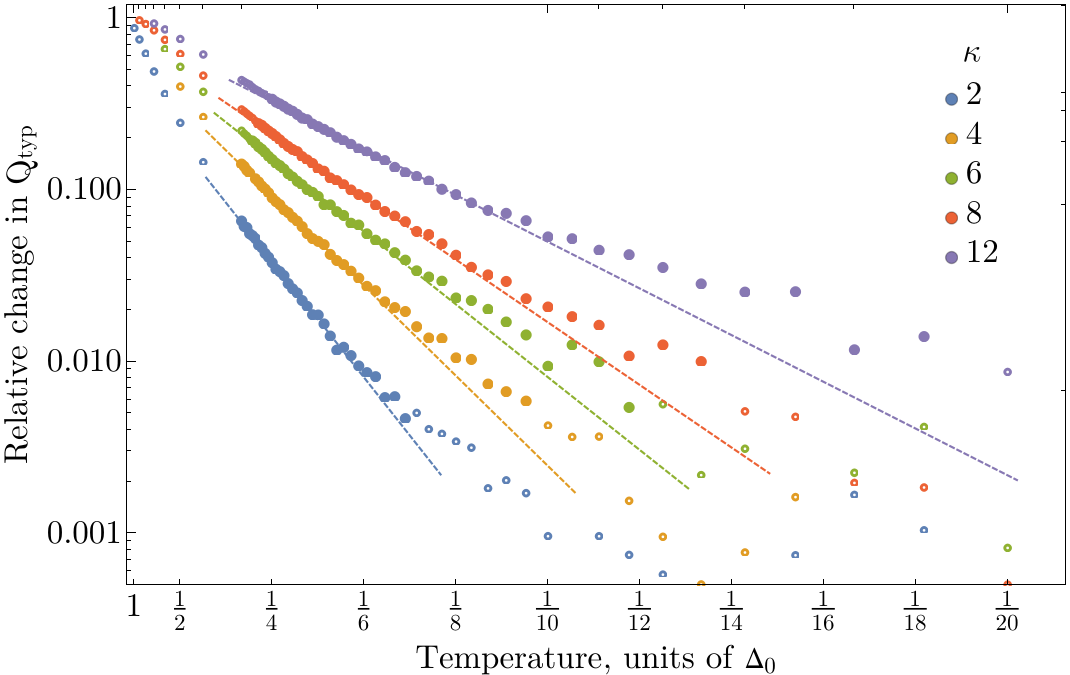
Figure 11: The temperature dependence of the relative change of typical local current response $1-Q_{\text{typ}}\left(T\right)/Q_{\text{typ}}\left(T=0\right)$ in logarithmic scale along the vertical axis and reciprocal ($1/T$) scale along the horizontal axis. Various colors correspond to various dimensionless disorder strength $\kappa$ and $K=15$. The temperature is measured in units of $\Delta_{0}$. The points with solid filling are selected according to the criteria $T\in\left[\lambda\left\langle\Delta\right\rangle,\lambda\left\langle\Delta\right\rangle+0.2\Delta_{0}\right]$ with $\left\langle\Delta\right\rangle$ being the mean order parameter at zero temperature. These highlighted points are used for exponential fitting $A\exp\left\{-T_{1}/T\right\}$, with the latter plotted with dashed lines.

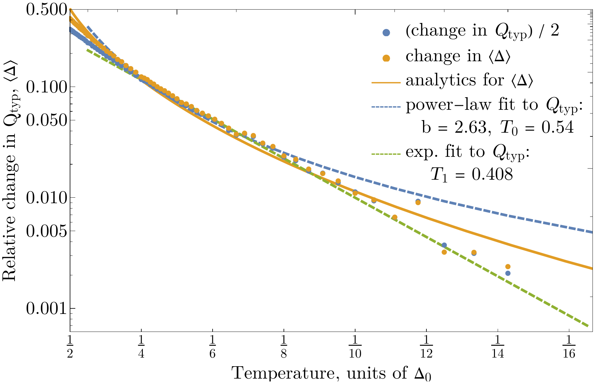
Figure 12: Low-temperature dependence of the relative changes in the typical local current response $1-Q_{\text{typ}}\left(T\right)/Q_{\text{typ}}\left(T=0\right)$ and the mean order parameter $1-\left\langle\Delta\right\rangle\left(T\right)/\left\langle\Delta\right\rangle\left(T=0\right)$ according to the numerical MPD (solid dots) and theoretical description given by Eqs. (48-49) (solid line). The values of $Q_{\text{typ}}$ are divided by two, according to relation (34). The dashed lines correspond to the power-law $\left(T/T_{0}\right)^{b}$ (blue) and activation-law $A\exp\left\{-T_{1}/T\right\}$ (green) fits and of numerical data for $Q_{\text{typ}}$ in the range $T\in\left[\lambda\left\langle\Delta\right\rangle,\lambda\left\langle\Delta\right\rangle+0.2\Delta_{0}\right]$, with $\left\langle\Delta\right\rangle=0.49\,\Delta_{0}$. The parameters of the model are $K=20,\,\kappa=10$.

We start by plotting on 11 the numerical data of 3 in logarithmic scale along the vertical axis and reciprocal scale $1/T$ along the horizontal axis. Similarly to the data processing of the main text, we then select a subset of points to apply the activation-law fit $\delta Q_{\text{typ}}/Q_{\text{typ}}=A\exp\left\{-T_{1}/T\right\}$ and plot the resulting curve. On 12 we also plot the data of 6 (both experimental and theoretical) with reciprocal scale of temperatures. The plot also features the activation-law fit of the numerical data. The latter appears to describe the data fairly well in a certain range of temperatures, similarly to what is seen on 3 in the main text.

The corresponding value of $T_{1}$ for various parameters is shown on 13. As $\kappa$ decreases, the value of $T_{1}$ increases and eventually approaches $2\Delta_{0}$ at small $\kappa$, as evident from 7 in the main text. At large $\kappa$, the value of $T_{1}$ can roughly be described by the typical order parameter $\Delta_{\text{typ}}=\exp\left\{\left\langle\ln\Delta\right\rangle\right\}$ at zero temperature, as suggested by 14. Note, however, that such a relation is not directly supported by the analytical approach of IV.2. Indeed, both $\delta Q_{\text{typ}}$ and $\Delta_{\text{typ}}$ are complicated functions of the parameters, and the temperature dependence of $\delta Q_{\text{typ}}$is not, in general, described by an activation law, so the relation $T_{1}\sim\Delta_{\text{typ}}$ is only empirical.

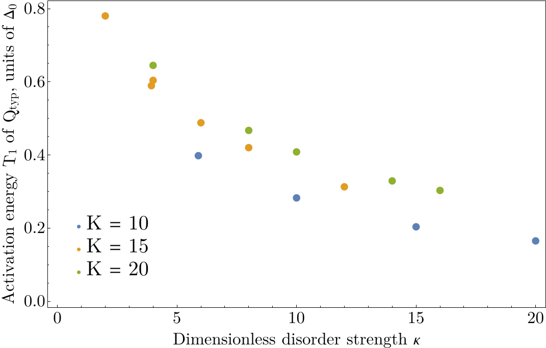
Figure 13: Dependence of the $T_{1}$ parameter of the activation-law fit $A\exp\left\{-T_{1}/T\right\}$ of the portion of numerical data for $\delta Q_{\text{typ}}\left(T\right)/Q_{\text{typ}}\left(0\right)$. For each set of parameters, the points for fitting are selected according to the criteria $T\in\left[\lambda\left\langle\Delta\right\rangle,\lambda\left\langle\Delta\right\rangle+0.2\Delta_{0}\right]$, with $\left\langle\Delta\right\rangle$ being the mean order parameter at zero temperature, so the dataset for $K=15$ corresponds to highlighted points on 11. The value of $\kappa$ was varied by changing the value of $\lambda$ while keeping $K$ constant, and various colors correspond to various values of $K$.

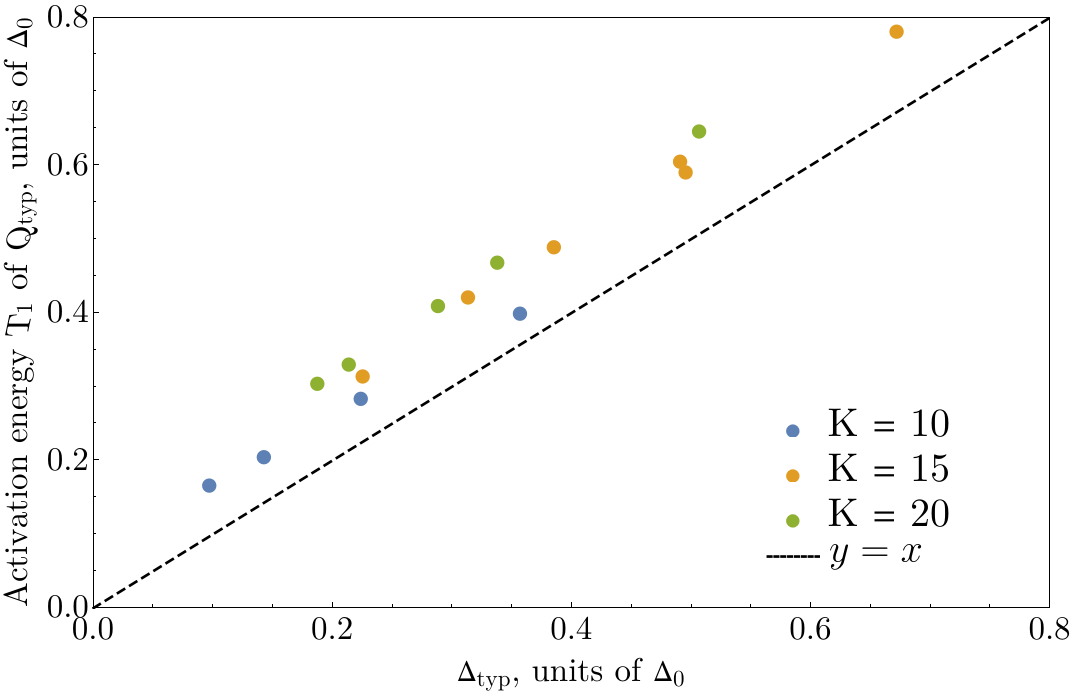
Figure 14: Comparison of the $T_{1}$ scale of the activation-law fit $A\exp\left\{-T_{1}/T\right\}$ from 13 with the typical order parameter $\Delta_{\text{typ}}=\exp\left\{\left\langle\ln\Delta\right\rangle\right\}$ at zero temperature for the same set of parameters $\kappa,K$ and $T=0$. The data points are the same as those presented on 13. The value of $\Delta_{\text{typ}}$ decreases with the increase of $\kappa$, thus giving the measure of disorder. The low-disorder case of 7 corresponds to $\left(\Delta_{\text{typ}}/\Delta_{0},T_{1}/\Delta_{0}\right)\approx\left(1,2\right)$ and thus does not fall into the apparent linear tendency.

Appendix E Restoring the superfluid stiffness $\Theta$ from the limit of small disorder

The order of magnitude of the $C$ constant in Eq. (24) can be estimated by examining the limit of weak disorder $\kappa\ll 1$ corresponding to large $K$. We first note that $Q$ scales as $1/K$, as can be seen e.g. from Eq. (32), so in order for $\Theta$ to remain finite as $K\rightarrow\infty$, the $C$ value should contain a factor of $K$. Moreover, in the limit of weak disorder the value of $Q_{\text{typ}}$ in Eq. (24) should be replaced by a simple average $\left\langle Q\right\rangle$. Indeed, in the limit of weak disorder one expects $\Theta$ to depend only on a local self-averaging quantity, and a natural choice for the latter with the correct dependence on $Q$ and $K$ is the sum of $Q$s over all neighbors of a given site.

The value of $\left\langle Q\right\rangle$ can then be evaluated directly, as it gains its value on configurations with $\xi_{1},\xi_{2}\gg\Delta$, so Eq. (32) is directly applicable with $E_{i}=\left|\xi_{i}\right|$. By cutting the logarithmic integrals over $\xi$ at $\Delta_{0}$ from below and $E_{F}$ from above one obtains

$$K\left\langle Q\right\rangle=\frac{\Delta_{0}\,\left(2e\right)^{2}}{c}\,\frac{2\nu_{0}\Delta_{0}}{\lambda n},$$ (87)

where $n$ is the concentration of sites. This results in the following expression for the superfluid density

$$\rho_{S}=\frac{C}{K}\,K\left\langle Q\right\rangle=\frac{C}{K}\,\frac{\Delta_{0}\,\left(2e\right)^{2}}{c}\,\frac{2\nu_{0}\Delta_{0}}{\lambda n}.$$ (88)

On the other hand, Ref. [45] provides an estimation of $\rho_{S}$ in a similar model:

$$\rho_{S}=\frac{2\nu_{0}e^{2}R_{0}^{2}}{\hbar}\left\langle\Delta\right\rangle^{2},$$ (89)

where $\left\langle\Delta\right\rangle\approx\Delta_{0}$ is the mean order parameter, $R_{0}\sim L_{0}\ln\frac{\delta_{\text{loc}}}{\Delta_{0}}\sim L_{0}/\lambda$, with $L_{0}$ being the interaction radius from III.1, and $\delta_{\text{loc}}=\left(\nu_{0}L_{0}^{3}\right)^{-1}$ being the level spacing in the localization volume. Comparing the two expressions, one arrives at

$$C\sim nR_{0}^{2}dK.$$ (90)

Appendix F The cross-Kerr effect in moderately disordered superconductors for a strip geometry

In this Appendix, we address the cross-Kerr coefficients for the plasmonic excitations in a moderately disordered superconductor (obeying semiclassical description). The latter is to be contrasted with the case of strongly disordered superconductors with a pseudogap discussed in Sections III and IV of the main text. We consider a strip of horizontal sizes $L\times w$ and thickness $d$ with the following hierarchy of scales $L\gg\lambda\gg w\gg d\gg\xi_{0}\gg l$, with $\lambda$ being the wavelength of the 1D plasmon in question, $\xi_{0}$ being the zero-temperature superconducting coherence length in the dirty limit, and $l$ being the mean free path. In particular, we assume both the charge and current density to be uniform across the thickness of the film. We also neglect the light retardation, i.e. the plasmon frequencies satisfies $\omega\ll c/\lambda$. For simplicity, we restrict our derivation to the case $T=0$.

The main source of non-harmonicity of the plasmonic modes is the nonlinearity of the current density response $\boldsymbol{j}$ to the vector potential $\boldsymbol{A}$. In the Coulomb gauge $\text{div}A=0$, the latter can be written as [29]

$$j\left(\boldsymbol{A}\right)=-\frac{\pi\sigma\Delta}{c}\left(1-\frac{4}{3\pi}\xi^{2}\left(\frac{2e}{\hbar c}\boldsymbol{A}\right)^{2}\right)\boldsymbol{A},$$ (91)

where $\sigma$ is the normal-state conductance, and $\xi=\sqrt{\hbar D/2\Delta}$ is the zero-temperature coherence length in terms of the diffusion constant $D$. The order parameter $\Delta$ also experiences a correction:

$$\Delta=\Delta_{0}\exp\left\{-\frac{\pi}{4}\xi^{2}\left(\frac{2e}{\hbar c}\boldsymbol{A}\right)^{2}\right\},$$ (92)

with $\Delta_{0}$ being the order parameter at $\boldsymbol{A}=0$ and $T=0$. The density of the kinetic energy is then obtained by integrating the current density (91) w.r.t the vector potential:

$$f_{\text{kin}}\left(\boldsymbol{A}\right) =-\frac{1}{c}\,\intop_{0}^{A}\left(\boldsymbol{j},d\boldsymbol{A}\right)$$

$$=\frac{\rho_{S}\boldsymbol{A}^{2}}{2c^{2}}\left(1-\frac{\alpha\xi^{2}}{2}\left(\frac{2e}{\hbar c}\boldsymbol{A}\right)^{2}+O\left(A^{4}\right)\right),$$ (93)

where in the last line we have used the standard relation $\rho_{S}=\pi\sigma\Delta_{0}$ for the dirty superconductor and expanded the result up to the leading powers of $\boldsymbol{A}^{2}$, yielding $\alpha=\frac{4}{3\pi}+\frac{\pi}{4}$, as a result of combining Eqs. (91) and (92). For the case of a thin film, the corresponding free energy reads

$$F_{\text{kin}}=\intop_{\text{volume}}d^{3}\boldsymbol{r}\,f_{\text{kin}}=d\,\intop_{\text{film}}d^{2}\boldsymbol{r}\,f_{\text{kin}},$$ (94)

where in the second line we assumed that $\boldsymbol{A}$ is uniform across the film’s thickness, and the integrations in the two expressions go over the film’s volume and surface, respectively.

The potential part of the plasmonic Hamiltonian is described by the electrostatic energy for a given charge density:

$$F_{\text{pot}}=\frac{1}{2}\iintop_{\text{film}}d^{2}\boldsymbol{r}d^{2}\boldsymbol{r}^{\prime}\,\,\rho\left(\boldsymbol{r}\right)V\left(\boldsymbol{r}-\boldsymbol{r}^{\prime}\right)\rho\left(\boldsymbol{r}^{\prime}\right),$$ (95)

where the integration goes over the surface of the film, $\rho$ is the 2D charge density, and $V\left(\boldsymbol{r}\right)$ is the electrostatic potential from a point charge (including the effects of screening from the ground plate and the substrate if present). The corresponding electrostatic potential reads [31]:

$$V\left(x,y\right) =\frac{4\pi}{1+\varepsilon}\frac{1}{\sqrt{x^{2}+y^{2}}}$$

$$-\frac{4\pi}{1+\varepsilon}\,\frac{2\varepsilon}{1+\varepsilon}\sum_{j=1}^{\infty}\frac{\left(\frac{1-\varepsilon}{1+\varepsilon}\right)^{j-1}}{\sqrt{x^{2}+y^{2}+\left(2hj\right)^{2}}}$$ (96)

where $h\gg d$ is the distance from the film to the ground plane, and $\varepsilon$ is the dielectric permittivity of the substrate. In what follows, we will neglect the screening, for simplicity, which amounts to assuming $h\sim L\gg w$.

The Hamiltonian of the plasmonic modes in the absence of retardation then reads

$$H =\frac{1}{2}\intop d^{2}\boldsymbol{r}d^{2}\boldsymbol{r}^{\prime}\,\rho\left(\boldsymbol{r}\right)V\left(\boldsymbol{r}-\boldsymbol{r}^{\prime}\right)\rho\left(\boldsymbol{r}^{\prime}\right)$$

$$+d\intop d^{2}\boldsymbol{r}\,f_{\text{kin}}\left(\frac{\hbar c}{2e}\nabla\varphi\right),$$ (97)

where $d$ is the film thickness, and the superconducting phase $\varphi$ is connected to the vector potential as $\boldsymbol{A}=\frac{\hbar c}{2e}\nabla\varphi$ (and also assumed to be uniform across the thickness of the film). The canonical commutation relations for the fields $\varphi,\rho$ take place:

$$\left[\varphi\left(\boldsymbol{r}\right),\rho\left(\boldsymbol{r}^{\prime}\right)\right]=\left(2e\right)i\,\delta\left(\boldsymbol{r}-\boldsymbol{r}^{\prime}\right).$$ (98)

At the boundary of the film, the field $\varphi$ should satisfy the condition $\left(\boldsymbol{n},\boldsymbol{j}\right)=0$, corresponding to the absence of the current through the edges of the film:

$$\left(n,\nabla\varphi\right)_{\boldsymbol{r}\in\text{boundary}}=0,$$ (99)

where $n$ is the normal vector to the boundary of the film. The Heisenberg’s equations of motion associated with Eq. (97) correspond to the charge conservation law and the Josephson’s relation:

$$\dot{\rho}=-\text{div}\boldsymbol{j},\,\,\,\dot{\varphi}\left(\boldsymbol{r}\right)=\frac{2e}{\hbar}\,\intop d^{2}\boldsymbol{r}^{\prime}\,V\left(\boldsymbol{r}-\boldsymbol{r}^{\prime}\right)\rho\left(\boldsymbol{r}^{\prime}\right).$$ (100)

By using the expansion (93) of $f_{\text{kin}}$ in powers of $\boldsymbol{A}$, we can rewrite the Hamiltonian (97) as

$$H =\frac{1}{2}\,\intop d^{2}\boldsymbol{r}d^{2}\boldsymbol{r}^{\prime}\,\rho\left(\boldsymbol{r}\right)V\left(\boldsymbol{r}-\boldsymbol{r}^{\prime}\right)\rho\left(\boldsymbol{r}^{\prime}\right)$$

$$+\frac{1}{2}\Theta\intop d^{2}\boldsymbol{r}\left(\nabla\varphi\right)^{2}\left[1-\frac{\alpha}{2}(\xi\nabla\varphi)^{2}+O\left((\xi\nabla\varphi)^{4}\right)\right],$$ (101)

where $\Theta=\rho_{S}d\,\left(\hbar/2e\right)^{2}$ is the 2D superfluid stiffness. Strictly speaking, the energy of phase fluctuations in Eqs. (97) and (101) also contains terms with higher derivatives of $\varphi$, such as, e.g., $\left(\xi\nabla^{2}\varphi\right)^{2}$, but those are responsible for the relative corrections of the order $O\left((k\xi)^{2}\right)$ to the plasmonic dispersion law, whereas we are interested in the leading nonlinearity w.r.t $\varphi$ that produces interaction of plasmons. As as a result, such terms can be neglected as far as the small frequencies and wave numbers are concerned.

F.1 Low-lying normal modes

To calculate the cross-Kerr coefficients, one first has to extract the normal modes of the Hamiltonian (101) in the absence of nonlinearity. The latter can be done by finding the oscillating solutions to the classical equations of motions (100):

$$\rho=e^{i\omega t}\rho_{\omega}\left(x,y\right),\,\,\,\varphi=e^{i\omega t}\varphi_{\omega}\left(x,y\right),$$ (102)

rendering

$$i\omega\rho_{\omega}=\rho_{S}d\,\frac{\hbar}{2e}\,\Delta\varphi,\,\,\,i\omega\varphi_{\omega}=\frac{2e}{\hbar}\,V\rho_{\omega},$$ (103)

where we introduced the shorthand $V\rho_{\omega}$ for the r.h.s. of the second relation in Eq. (100) for brevity. For a given set of solutions $\left\{\omega,\rho_{\omega},\varphi_{\omega}\right\}$ with positive angular frequencies $\omega>0$, the harmonic part of the plasmonic Hamiltonian (101) is rewritten as

$$H=\sum_{\omega}\hbar\omega\,\left(\alpha_{\omega}^{\dagger}\alpha_{\omega}+\frac{1}{2}\right),$$ (104)

where $\alpha_{\omega}^{\dagger},\,\alpha_{\omega}$ are the creation and annihilation operators of the plasmonic modes satisfying the standard bosonic commutation relations, and the field operators are then expressed as

$$\rho\left(x,y\right)=\sum_{\omega}\sqrt{\frac{\hbar\omega}{\rho_{\omega}V\rho_{\omega}}}\,\frac{\alpha_{\omega}-\alpha_{\omega}^{\dagger}}{\sqrt{2}i}\,\rho_{\omega}\left(x,y\right),$$ (105)

$$\varphi\left(x,y\right)=\sum_{\omega}\sqrt{\frac{2e}{i\varphi_{\omega}\rho_{\omega}}}\frac{\alpha_{\omega}+\alpha_{\omega}^{\dagger}}{\sqrt{2}\,}\,i\varphi_{\omega}\left(x,y\right).$$ (106)

where denoted $\varphi_{\omega}\rho_{\omega}=\intop d^{2}\boldsymbol{r}\,\varphi_{\omega}\left(\boldsymbol{r}\right)\rho_{\omega}\left(\boldsymbol{r}\right)$ and $\rho_{\omega}V\rho_{\omega}=\intop d^{2}\boldsymbol{r}\,d^{2}\boldsymbol{r}^{\prime}\,\rho_{\omega}\left(\boldsymbol{r}\right)\,V\left(\boldsymbol{r}-\boldsymbol{r}^{\prime}\right)\rho_{\omega}\left(\boldsymbol{r}\right)$ for brevity.

For the low-lying modes in the strip geometry, one can perform the plain wave ansatz:

$$\rho_{\omega}=\sqrt{\frac{2}{L}}\cos kx\,\rho_{k}\left(y\right),\,\,\,\varphi_{\omega}=\sqrt{\frac{2}{L}}\cos kx\,\varphi_{k}\left(y\right),$$ (107)

with $\partial_{y}\varphi_{k}\left(\pm w/2\right)=0$ as a result of the boundary conditions (99). This leads to the following system of equations for the profile of the plasmon in the perpendicular direction:

$$i\omega\rho_{k}\left(y\right)=\rho_{S}d\,\frac{\hbar}{2e}\,\left(-k^{2}+\partial_{y}^{2}\right)\varphi_{k},$$ (108)

$$i\omega\varphi_{k}\left(y\right)=\frac{2e}{\hbar}\,\intop_{-w/2}^{w/2}dy^{\prime}\,V_{k}\left(y-y^{\prime}\right)\,\rho_{k}\left(y^{\prime}\right),$$ (109)

$$V_{k}\left(y\right)=\intop_{-\infty}^{\infty}dx\,e^{ikx}\,V\left(x,y\right).$$ (110)

The system (108-110) can be solved analytically for the case of the potential (96) in the limit $kw\ll 1$ and $w\ll h$. We start by discussing the static limit $k\rightarrow 0$, as it formally corresponds to the electrostatic problem for the same geometry. The charge distribution is then found from the electroneutrality condition $\boldsymbol{E}=0$:

$$\partial_{y}\,\intop_{-w/2}^{w/2}dy^{\prime}\,V_{0}\left(y-y^{\prime}\right)\,\rho_{0}\left(y^{\prime}\right)=0,$$ (111)

where we have used only the $y$-component of the electric field, as the $x$ component vanishes automatically in the static limit: $\partial_{x}V\rho\sim k\,V\rho\rightarrow 0$. In the limit $k\rightarrow 0$, the Fourier transform (110) of the electrostatic potential (96) reads:

$$V_{0}\left(y\right) =\frac{4\pi}{1+\varepsilon}\left[-\frac{2\varepsilon}{1+\varepsilon}\sum_{j=1}^{\infty}\,\left(\frac{1-\varepsilon}{1+\varepsilon}\right)^{j-1}\,2\ln\frac{w/2}{2hj}\right]$$

$$+\frac{4\pi}{1+\varepsilon}\left[2\ln\frac{w/2}{\left|y\right|}+O\left(\left(\frac{y}{h}\right)^{2}\right)\right],$$ (112)

where in the second line we have taken into account that $w\ll h$.

In the absence of screening, i.e., $h\rightarrow\infty$, Eq. (111) can be solved exactly:

$$\rho_{0}\left(y\right)=\frac{C}{\sqrt{\left(w/2\right)^{2}-y^{2}}},$$ (113)

where $C$ is a normalization constant. The corrections from finite $h$ can be retrieved by formal expansion in even Chebyshev polynomials:

$$\rho_{0}\left(y\right)=\frac{1}{\sqrt{\left(w/2\right)^{2}-y^{2}}}\,\sum_{n=0}^{\infty}\rho^{\left(n\right)}T_{2n}\left(2y/w\right),$$ (114)

with $\rho^{\left(n\right)}=O\left(\left[\frac{w}{2h}\right]^{2n}\right)$. For instance,

$$\rho^{\left(0\right)}=C,\,\,\,\rho^{\left(1\right)}=-C\left(\frac{w}{2h}\right)^{2}\frac{1}{16}\,\frac{2\varepsilon}{1-\varepsilon}\text{Li}_{2}\left(\frac{1-\varepsilon}{1+\varepsilon}\right),$$ (115)

where $\text{Li}_{n}\left(z\right)=\sum_{k=1}^{\infty}z^{k}/k^{n}$ is the the polylogarithm function, and $C$ is the normalization constant. In what follows, we will ignore those corrections.

At finite $k$, the charge distribution $\rho_{k}\left(y\right)$ perturbatively deviates from its static profile $\rho_{0}\left(y\right)$, so we can find the leading approximation for the phase profile $\varphi_{k}$ by using the Josephson’s relation 109 with the unperturbed value of the charge distribution:

$$\varphi_{k} =\frac{1}{i\omega_{k}}\,\frac{2e}{\hbar}\,\intop_{-w/2}^{w/2}dy^{\prime}\,V_{k}\left(y-y^{\prime}\right)\,\rho_{k}\left(y^{\prime}\right)$$

$$\approx\frac{1}{i\omega_{k}}\,\frac{2e}{\hbar}\,\intop_{-w/2}^{w/2}dy^{\prime}\,V_{k}\left(y-y^{\prime}\right)\,\rho_{0}\left(y^{\prime}\right),$$ (116)

By construction, the last expression is constant at $k\rightarrow 0$, so the leading approximation the phase is distributed uniformly. The exact value of $\varphi_{k}$ can then be found by integrating the charge conservation (108):

$$\varphi_{k}\approx-\frac{i\omega_{k}}{k^{2}w}\,\intop_{-w/2}^{w/2}dy\,\rho_{0}\left(y\right)=-\frac{i\omega_{k}\,\pi C}{\rho_{S}d\,\frac{\hbar}{2e}\,k^{2}w}.$$ (117)

It is instructive to follow how the charge conservation (108) is respected given the singular profile (113) of the charge density and nearly constant profile of the phase. The singularity in the charge profile is compensated by a small but singular corrections to $\varphi_{k}$ at finite $k$:

$$\varphi_{k}=C_{k}+\omega_{k}\left[1-\left(\frac{y}{w/2}\right)^{2}\right]^{3/2}f_{k}\left(y\right),$$ (118)

where the constant term $C_{k}$ is given by Eq. (117), and $f\left(y\right)$ is a regular function of $y$ that weakly depends on $k$ at $k\rightarrow 0$. Plugging this expression in the r.h.s Eq. (108) renders a singular term identical to the one present in the l.h.s.

Demanding the two Eqs. (116) and (117) to be consistent then delivers the plasmonic spectrum:

$$\omega_{k}^{2}=\rho_{S}d\,k^{2}\,\frac{\intop_{-w/2}^{w/2}dy^{\prime}\,V_{k}\left(y-y^{\prime}\right)\,\rho_{0}\left(y^{\prime}\right)}{\intop_{-w/2}^{w/2}dy\,\rho_{0}\left(y\right)},$$ (119)

where we have retained the $k$-dependence in $V_{k}$ as it contains the weak logarithmic correction to the leading approximation. Using the exact profile (96) of the electrostatic potential, one obtains asymptotic behavior of the result in the two limiting cases:

$$\omega_{k}^{2}=\begin{cases}\frac{8\pi}{1+\varepsilon}\,\rho_{S}dk^{2}w\,\ln\frac{8h}{we^{\delta\left(\varepsilon\right)}},&k\ll h^{-1},\\ \frac{8\pi}{1+\varepsilon}\rho_{S}dk^{2}w\,\ln\frac{8}{kwe^{\gamma}},&w^{-1}\gg k\gg h^{-1},\end{cases}$$ (120)

where $\gamma=0.577...$ is the Euler-Mascheroni constant, and $\delta\left(\varepsilon\right)$ is defined as

$$\delta\left(\varepsilon\right)=\frac{2\varepsilon}{1+\varepsilon}\sum_{j=1}^{\infty}\,\left(\frac{1-\varepsilon}{1+\varepsilon}\right)^{j-1}\,\ln\frac{1}{j}.$$ (121)

Note, in particular, that the logarithmic correction to the 1D plasmon dispersion law at $w^{-1}\gg k\gg h^{-1}$ has been predicted theoretically [26] and observed experimentally [27, 28], with the latter being in perfect agreement, including the numeric coefficient inside the logarithm. Corrections to $\omega_{k},\,\rho_{k},\,\varphi_{k}$ for $h\sim w$ and/or $kw\sim 1$ can be studied numerically, as has been done to verify the presented results.

F.2 Cross-Kerr coefficients

We can now expand the leading anharmonic part of the Hamiltonian in harmonic modes, according to Eq. (117):

$$\delta H =-\frac{\alpha}{4}\,\Theta\xi^{2}\,\intop d^{2}r\,\left|\nabla\varphi\right|^{4}$$

$$=-\sum_{\left\{\omega_{i}\right\}}\eta_{\left\{\omega_{i}\right\}}\prod_{i}\left(\alpha_{\omega_{i}}+\alpha_{\omega_{i}}^{\dagger}\right)$$ (122)

where

$$\eta_{\left\{\omega_{i}\right\}} =\frac{\alpha}{4}\,\Theta\xi^{2}\,\left(\prod_{i=1}^{4}\,\frac{1}{\sqrt{2}}\sqrt{\frac{2e}{i\intop dr\,\varphi_{i}\rho_{i}}}\right)$$

$$\,\,\,\intop d^{2}r\,\left(\nabla\varphi_{1},\nabla\varphi_{2}\right)\left(\nabla\varphi_{3},\nabla\varphi_{4}\right).$$ (123)

The calculation of the cross-Kerr effect is then similar to that of Ref. [30, Appendix B]. We substitute the particular form, Eqs. (107), (113), and (117), of the $\varphi,\rho$ vectors, rendering a simple expression:

$$\eta_{\left\{\omega_{i}\right\}}=\frac{\alpha}{4}\Theta\,\frac{2\xi^{2}}{Lw}\left(\prod_{i=1}^{4}\sqrt{\frac{\hbar\omega_{i}}{\Theta}}\right)\frac{1}{L}\intop dx\,\prod_{i}\sin k_{i}x.$$ (124)

In particular, $\eta_{i}$ has complete symmetry w.r.t permutations. We can then expand the sum in Eq. (122) according to the number of coinciding frequencies:

$$\delta H =-\sum_{\omega}\eta_{\omega\omega\omega\omega}\left(\alpha_{\omega}+\alpha_{\omega}^{\dagger}\right)^{4}$$

$$-3\sum_{\omega\neq\nu}\eta_{\omega\omega,\nu\nu}\left(\alpha_{\omega}+\alpha_{\omega}^{\dagger}\right)^{2}\left(\alpha_{\nu}+\alpha_{\nu}^{\dagger}\right)^{2}$$

$$-4\sum_{\omega\neq\nu}\eta_{\omega\omega\omega\nu}\left(\alpha_{\omega}+\alpha_{\omega}^{\dagger}\right)^{3}\left(\alpha_{\nu}+\alpha_{\nu}^{\dagger}\right)$$

$$-6\sum_{\omega\neq\nu,\theta\neq\omega,\nu}\eta_{\omega\omega\nu\theta}\left(\alpha_{\omega}+\alpha_{\omega}^{\dagger}\right)^{2}\left(\alpha_{\nu}+\alpha_{\nu}^{\dagger}\right)\left(\alpha_{\theta}+\alpha_{\theta}^{\dagger}\right)$$

$$-\sum_{\text{all }\omega_{i}\text{ diff.}}\underset{0,\text{ momentum conservation}}{\underbrace{\eta_{\left\{\omega_{i}\right\}}}}\prod_{i}\left(\alpha_{\omega_{i}}+\alpha_{\omega_{i}}^{\dagger}\right).$$ (125)

To describe the cross-Kerr effect by this expression, we pick out only terms that map any two-excitation state to itself. The result reads

$$\delta H \mapsto-\sum_{\omega}\eta_{\left\{\omega\right\}}\left[6n_{\omega}^{2}+6n_{\omega}+3\right]$$

$$-3\sum_{\omega,\nu\neq\omega}\eta_{\omega\omega,\nu\nu}\left[4n_{\omega}n_{\nu}+2n_{\omega}+2n_{\nu}+1\right]$$ (126)

We can finally rewrite this as

$$\delta H=\sum_{\omega}\delta\omega\,\left(n_{\omega}+\frac{1}{2}\right)-\frac{1}{2}\sum_{\omega,\nu}K_{\omega\nu}n_{\omega}n_{\nu},$$ (127)

where

$$K_{\omega\nu}=12\left(2-\delta_{\omega\nu}\right)\eta_{\omega\omega\nu\nu},$$ (128)

$$\delta\omega=-\frac{1}{2}K_{\omega\omega}-\frac{1}{4}\sum_{\nu\neq\omega}K_{\omega\nu}.$$ (129)

The relevant values of $\eta$ then read

$$\eta_{\omega\omega\nu\nu}=\Theta\,\left(1+\frac{1}{2}\delta_{\omega\nu}\right)\,\frac{1}{4}\,\frac{\alpha}{4}\,\frac{2\xi^{2}}{Lw}\,\frac{\hbar\omega}{\Theta}\,\frac{\hbar\nu}{\Theta},$$ (130)

rendering the final result for the cross-Kerr coefficients $K_{\omega\nu}$:

$$K_{\omega\nu}=3\alpha\left(1-\frac{1}{4}\delta_{\omega\nu}\right)\,\Theta\,\frac{\xi^{2}}{Lw}\,\frac{\hbar\omega}{\Theta}\,\frac{\hbar\nu}{\Theta},$$ (131)

where the value of $\alpha=\frac{3}{4\pi}+\frac{\pi}{4}\approx 1.02$ originates from the particular form of the nonlinearity of the current-phase relation (93) in moderately disordered superconductors.

The result (131) can be qualitatively compared to that for a chain of Josephson junctions with short-range capacitive coupling from Ref. [31]. In the latter case, the nonlinearity in the current-phase relation is described by $\sin x\approx x-x^{3}/6\Rightarrow\alpha=1/6$, and the factor $N$ in [31, Eq. (14)] corresponds to $Lw/2\xi^{2}$.

We finally remind the reader that this result is only applicable to the case of moderately disordered superconductors described by semiclassical approximation. In contrast, the current-phase nonlinearity in strongly disordered superconductors with a pseudogap is yet to be described theoretically.