A Universal Model of Floquet Operator Krylov Space

Abstract

It is shown that the stroboscopic time-evolution under a Floquet unitary, in any spatial dimension, and of any Hermitian operator, can be mapped to an operator Krylov space which is identical to that generated by the edge operator of the non-interacting Floquet transverse-field Ising model (TFIM) in one-spatial dimension, and with inhomogeneous Ising and transverse field couplings. The latter has four topological phases reflected by the absence (topologically trivial) or presence (topologically non-trivial) of edge modes at $0$ and/or $\pi$ quasi-energies. It is shown that the Floquet dynamics share certain universal features characterized by how the Krylov parameters vary in the topological phase diagram of the Floquet TFIM with homogeneous couplings. These results are highlighted through examples, all chosen for numerical convenience to be in one spatial dimension: non-integrable Floquet spin $1/2$ chains and Floquet $Z_{3}$ clock model where the latter hosts period-tripled edge modes.

Introduction.—The nonequilibrium dynamics of interacting quantum systems is a challenging problem as few non-perturbative analytic methods exist, and exact numerical simulations are restricted to small system sizes. Recently, the study of operator dynamics in Krylov space [1, 2, 3, 4, 5, 6], has emerged as a powerful method because this approach maps an interacting problem to a non-interacting one, making it amenable to a host of methods valid for single particle quantum mechanics [7, 8, 9]. However, this approach has been primarily applied to continuous time evolution, where the operator Krylov space corresponds to a single particle hopping on a tight-binding lattice with nearest-neighbor and inhomogeneous hopping. Extending Krylov methods to Floquet systems [10, 11, 12] is particularly important as Floquet dynamics is qualitatively different from continuous time dynamics because energy is conserved in the former only up to integer multiples of the driving frequency [13, 14], resulting in spectra that are $2\pi$ periodic. This periodicity is behind novel phenomena such as new topological phases with no counterpart in continuous time evolution [15, 16, 17, 18, 19, 20, 21, 22, 23, 24, 25, 26].

In this work we derive a remarkably simple operator Krylov space picture under stroboscopic (Floquet) time evolution. We show that the Krylov space of any Hermitian operator under Floquet dynamics, independent of the spatial dimension, is identical to the Krylov space of a non-interacting problem in one dimension. The latter is the Floquet transverse field Ising model with inhomogeneous couplings (ITFIM). For homogeneous couplings, the Floquet transverse field Ising model (TFIM) is well documented as having four topological phases [27, 19, 26, 28]: a trivial phase with no edge modes, a $0$ ($\pi$)-mode phase with an edge mode at zero ($\pi$) quasi-energy, and a $0$-$\pi$ phase where both $0$ and $\pi$ edge modes exist together. We show that all operator dynamics in Krylov space can be mapped to the edge mode dynamics of a suitable ITFIM. In addition, the dynamics has certain universal features reflected in the trajectory that the inhomogeneous couplings take in the topological phase diagram of the TFIM, on moving from the edge to the bulk of the Krylov chain. This allows us to capture the exact dynamics quite faithfully, at least at short and intermediate times, by employing a much smaller number of Krylov parameters than the size of the Hilbert space.

Operator Krylov Space from a Floquet Unitary.—In order to construct the Floquet Krylov space for a given operator, one follows the Arnoldi iteration [29]. One begins with an initial operator $O_{0}$ and then generates new operators via the Floquet unitary $U$. Finally, a set of orthonormal operators $\{\mathcal{O}_{i}\}$ are generated by the Gram-Schmidt process. Explicitly, one initially sets $\mathcal{O}_{0}=O_{0}$ and performs the algorithm below for an integer $i>0$

$$|\mathcal{O}_{i}^{\prime})=K|\mathcal{O}_{i-1})-\sum_{j=1}^{i-1}|\mathcal{O}_{j})(\mathcal{O}_{j}|K|\mathcal{O}_{i-1});$$ (1)

$$|\mathcal{O}_{i})=\frac{|\mathcal{O}_{i}^{\prime})}{\sqrt{(\mathcal{O}_{i}^{\prime}|\mathcal{O}_{i}^{\prime})}},$$ (2)

where $|\mathcal{O}_{i})$ is the vector representation of $\mathcal{O}_{i}$ and $K|\mathcal{O}_{i})=U^{\dagger}\mathcal{O}_{i}U$. The inner product of two operators is defined as $(A|B)=\text{Tr}[A^{\dagger}B]/N$, where $A$ and $B$ are $N\times N$ matrices, with $N$ being the size of Hilbert space. $K$ has an upper-Hessenberg form $(\mathcal{O}_{i}|K|\mathcal{O}_{j})=0$ for $i>j+1$ [10, 12]. In addition, Ref. [12] showed that $K$ has the following simple structure parameterized by $\{a_{i}\}$, $\{b_{i}\}$ and $\{c_{i}\}$ in the orthonormal bases $\{|\mathcal{O}_{i})\}$:

$$b_{i}=(\mathcal{O}_{i}|K|\mathcal{O}_{i-1}); \frac{a_{i}}{c_{i}}c_{j}=(\mathcal{O}_{i}|K|\mathcal{O}_{j})\ \text{for}\ i\leq j,$$ (3)

where $a_{0}=c_{0}$. For example, $K$ has the following explicit expression for $N=6$,

$$K=\begin{pmatrix}a_{0}&c_{1}&c_{2}&c_{3}&c_{4}&c_{5}\\ b_{1}&a_{1}&\frac{a_{1}}{c_{1}}c_{2}&\frac{a_{1}}{c_{1}}c_{3}&\frac{a_{1}}{c_{1}}c_{4}&\frac{a_{1}}{c_{1}}c_{5}\\ 0&b_{2}&a_{2}&\frac{a_{2}}{c_{2}}c_{3}&\frac{a_{2}}{c_{2}}c_{4}&\frac{a_{2}}{c_{2}}c_{5}\\ 0&0&b_{3}&a_{3}&\frac{a_{3}}{c_{3}}c_{4}&\frac{a_{3}}{c_{3}}c_{5}\\ 0&0&0&b_{4}&a_{4}&\frac{a_{4}}{c_{4}}c_{5}\\ 0&0&0&0&b_{5}&a_{5}\end{pmatrix}.$$ (4)

If the initial operator $O_{0}$ is Hermitian, the orthonormal operators $\{\mathcal{O}_{i}\}$ are also Hermitian which implies $\{a_{i}\}$, $\{b_{i}\}$ and $\{c_{i}\}$ are all real numbers. With the condition of unitarity, $K$ is an orthogonal matrix, $K^{\intercal}K=\mathbb{I}$, and $\{a_{i}\}$, $\{b_{i}\}$ and $\{c_{i}\}$ are not independent variables. In particular, we show that the following relations hold between the matrix elements [30]

$$a_{i}=\cos\theta_{i}\cos\theta_{i+1}; b_{i}=\sin\theta_{i};$$

$$c_{i}=(-1)^{i}\cos\theta_{i+1}\prod_{j=1}^{i}\sin\theta_{j},$$ (5)

where $\theta_{0}=\theta_{N}=0$. This is consistent with the numerical observation in [12] that $|a_{i}|$, $|b_{i}|$, $|c_{i}|\leq 1$. Essentially, all the information of the Floquet Krylov space is encoded in the Krylov angles $\{\theta_{i}\}$, which can be derived from computing only the $\{a_{i}\}$ and $\{b_{i}\}$.

A Universal Model.—Identical matrix elements of $K$ in Krylov space, or equivalently $\{a_{i}\}$, $\{b_{i}\}$ and $\{c_{i}\}$ in (5), can be generated by the ITFIM with open boundary conditions

$$U_{\text{ITFIM}}=U_{z}U_{xx},$$ (6)

with

$$U_{z}=\prod_{j=1}^{N/2}e^{-i\frac{\theta_{2j-1}}{2}\sigma_{j}^{z}};U_{xx}=\prod_{j=1}^{(N-2)/2}e^{-i\frac{\theta_{2j}}{2}\sigma_{j}^{x}\sigma_{j+1}^{x}},$$ (7)

where we assume $N$ is even, and the boundaries are at $j=1,N/2$. The Krylov angle $\theta_{2j-1}$ ($\theta_{2j}$) corresponds to the local transverse-field (Ising coupling) of the model. This is a non-interacting system since $U_{\text{ITFIM}}$ is bilinear in Majorana fermions $\gamma_{\ell},\ell\in 1,\ldots,N$. By constructing the Krylov space of the edge Majornana $\gamma_{1}$ undergoing Floquet evolution due to $U_{\text{ITFIM}}$, the $K_{\text{ITFIM}}$ in the Krylov space orthonormal basis has the exact same matrix elements as the $K$ in (3) and (5). This can be checked directly by symbolic computation in Mathematica. We emphasize that this mapping is always valid regardless of the spatial dimension, or local Hilbert space of the original model. Therefore, the study of the autocorrelation function of some Hermitian operator $O_{0}$ in any Floquet model is equivalent to the study of the autocorrelation function of the edge Majorana $\gamma_{1}$, in the non-interacting Floquet ITFIM with local couplings $\{\theta_{i}\}$. Since this mapping is at the level of operator evolution, the equivalence also extends to objects beyond autocorrelation functions, such as operator entanglement.

Figure 1: Top panels: Infinite temperature autocorrelation function of the edge spin $\sigma_{1}^{x}$ for the unitary (8) in four different topological phases, $0$-mode, $\pi$-mode, $0$-$\pi$-mode and trivial from left to right, and from ED for $L=12,14$. Bottom panels: Krylov angles for the same, for $L=8,10,12$. $K_{\text{ITFIM}}$ is truncated to a $50\times 50$ matrix and constructed from the Krylov angles for $L=12$. The corresponding autocorrelation obtained as a return amplitude, (14) (green lines in top panels), and from further approximations, (15) (red lines in the top panels) show good agreement with ED. This supports the physical picture that the long-lived autocorrelation is an approximate edge mode of the ITFIM, and that the survival of the edge mode is related to the segment in Krylov space where the angle $\theta_{i}$ is confined within the relevant topological phase.

To demonstrate this mapping, we study the following models, all chosen in one-dimension for numerical convenience. The first model corresponds to an open spin $1/2$ chain with $L$ sites:

$$U_{1}=e^{-i\frac{T}{2}J_{z}H_{zz}}e^{-i\frac{T}{2}gH_{z}}e^{-i\frac{T}{2}J_{x}H_{xx}};$$ (8)

where

$$H_{xx}=\sum_{i=1}^{L-1}\sigma_{i}^{x}\sigma_{i+1}^{x};H_{zz}=\sum_{i=1}^{L-1}\sigma_{i}^{z}\sigma_{i+1}^{z};H_{z}=\sum_{i=1}^{L}\sigma_{i}^{z}.$$ (9)

$U_{1}$ is the Floquet TFIM perturbed by a transverse Ising interaction $J_{z}\neq 0$. The second model is the generalization of the TFIM to the $Z_{3}$ clock model [31]

$$U_{2}=e^{-i\frac{T}{2}H_{h}}e^{-i\frac{T}{2}H_{J}},$$ (10)

where

$$H_{J}=J\sum_{i=1}^{L-1}\sigma_{i}\sigma_{i+1}^{\dagger}+\text{H.c.}; H_{h}=h\sum_{i=1}^{L}\tau_{i}+\text{H.c.},$$ (11)

$$\sigma=\begin{pmatrix}1&0&0\\ 0&e^{i2\pi/3}&0\\ 0&0&e^{i4\pi/3}\end{pmatrix}; \tau=\begin{pmatrix}0&0&1\\ 1&0&0\\ 0&1&0\end{pmatrix}.$$ (12)

We study the above models with open boundary conditions because these models host long lived edge modes, and hence have non-trivial autocorrelation functions. To further support the applicability of ITFIM, we also study the autocorrelation function of an edge and a bulk spin for the Floquet transverse-field XYZ model [30]. Note that the Hilbert spaces of the model we are studying and the effective model to which the Krylov dynamics maps, ITFIM, may be completely different as highlighted from the example of the $Z_{3}$ clock model.

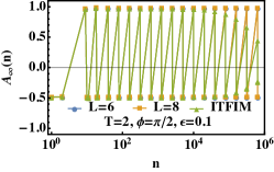
Results and Discussion.—We compute the infinite temperature autocorrelation function by exact diagonalization (ED),

$$A_{\infty}(n)=\frac{1}{N}\text{Tr}[O_{0}(n)O_{0}].$$ (13)

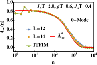
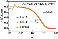
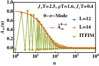
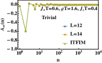
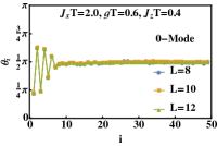
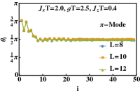
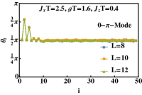
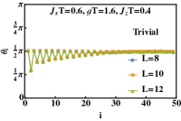
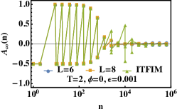
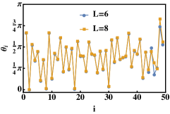
For $U_{1}$ (8), we take the seed operator to be the edge operator $O_{0}=\sigma_{1}^{x}$ and we take $gT,J_{x}T$ in (8) to lie within the four different topological phases of the Floquet TFIM, (triangles in Fig. 2). These are phases that host a $0$-mode ($J_{x}T=2.0$ and $gT=0.6$), a $\pi$-mode ($J_{x}T=2.0$ and $gT=2.5$), $0$-$\pi$-modes ($J_{x}T=2.5$ and $gT=1.6$) and a trivial phase with no edge modes ($J_{x}T=0.6$ and $gT=1.6$). We take the strength of the integrability breaking perturbation to be $J_{z}=0.4$. Due to the perturbation, the edge modes are almost strong modes [28, 26, 10, 32, 33, 34] where the autocorrelation decays to zero at a system size independent, albeit long time (top panels of Fig. 1). The Krylov angles of these four setups are shown in the lower panels of Fig. 1, where the angles approach $\pi/2$ in the bulk of the Krylov chain. Since the full Hilbert space size is $N=2^{L}$, it is impractical to exhaust all Krylov angles numerically. Therefore, we truncate $K_{\text{ITFIM}}$ into a $50\times 50$ matrix and construct its matrix elements from the Krylov angles for $L=12$. We set the boundary condition of the truncation as $\theta_{0}=0$ and $\theta_{50}=\pi/2$. Due to the truncation, $K_{\text{ITFIM}}^{\intercal}K_{\text{ITFIM}}$ is not equal to identity. Instead, it is a diagonal matrix in Krylov space with matrix elements $(1,\ldots,1,0)$ along the diagonal. The autocorrelation can also be computed from the $K_{\text{ITFIM}}$ from the relation

$$A_{\infty}(n)=(K_{\text{ITFIM}}^{n})_{1,1}.$$ (14)

Above $(K_{\text{ITFIM}}^{n})_{1,1}$ is the upper left-most matrix element of $K_{\text{ITFIM}}^{n}$. (14) encodes the equivalence between the autocorrelation in ED and the return amplitude of the edge Majorana of the ITFIM after $n$ periods. Here we are actually computing $(K_{\text{ITFIM}}^{n})_{1,1}$ in the single Majorana basis since ITFIM is bilinear in Majoranas and $K_{\text{ITFIM}}$ is a sparse matrix in the single Majorana basis. Fig. 1 shows that $K_{\text{ITFIM}}$ captures the initial decay of the autocorrelation from ED, while it decays to zero somewhat faster than ED due to the truncation of $K_{\text{ITFIM}}$.

Figure 2: The trajectory of local couplings from the edge to the bulk for the ITFIM, where $\theta_{2j-1}$ ($\theta_{2j}$) corresponds to the local transverse-field $g_{j}T$ (Ising coupling $J_{xj}T$). The Krylov angles are for $L=12$, for model (8), with the black crosses denoting the local couplings on the first Krylov site. The four triangles mark the non-perturbed limit ($J_{z}=0$) of the top panels in Fig. 1. The perturbation leads to inhomogeneous couplings. The local couplings on the first site take values close to the unperturbed limit. In contrast, in the bulk, the local couplings approach $\pi/2$ (bottom panels in Fig. 1). The phase diagram shows that the autocorrelation will eventually decay since the couplings in the bulk cannot allow for the existence of edge modes.

Figure 3: Infinite temperature autocorrelation functions (left panels) for the $Z_{3}$ clock model (10) with $O_{0}=(\sigma_{1}+\sigma_{1}^{\dagger})/\sqrt{2}$, $T=2$, $J=e^{i\phi}$ and $h=\epsilon+i2\pi/(3\sqrt{3})$. Also shown are Krylov angles (middle panels) and the corresponding ITFIM couplings in the phase diagram of the TFIM. The black cross (right panels) indicates the Krylov angle on the first site. Top panels: the autocorrelation shows the presence of a long-lived edge mode at $\phi=\pi/2$,$\epsilon=0.1$. Although the Krylov angles approach $\pi/2$, the system still supports a long-lived period tripled edge mode in contrast to previous examples. Bottom panels: the autocorrelation with tripled period decays much faster, and shows no long lived edge mode for $\phi=0,\epsilon=0.001$. The Krylov angles do not approach $\pi/2$ and the trajectory in the phase diagram initially meanders in the trivial phase. $K_{\text{ITFIM}}$ is truncated to a $50\times 50$ matrix and constructed from Krylov angles for $L=8$. The ITFIM fails to capture the late-time dynamics in both cases in the left panels, indicating that more Krylov angles are needed to capture the late time behavior.

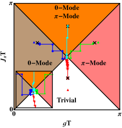
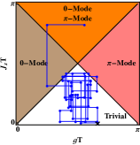
One can represent the mapping between the original model and the ITFIM in the phase diagram of the Floquet TFIM with homogeneous couplings, as shown in Fig. 2. After mapping to ITFIM, the Krylov angles $\{\theta_{i}\}$ are identified as local transverse-fields, $g_{i}T=\theta_{2i-1}$, and local Ising couplings, $J_{xi}T=\theta_{2i}$. One constructs a series of data points, $(g_{1}T,J_{x1}T),(g_{2}T,J_{x1}T),(g_{2}T,J_{x2}T),(g_{3}T,J_{x2}T)\ldots$, and this trajectory is plotted in the phase diagram. In particular, one finds that the couplings from the edge to the bulk gradually deviate from the original phase in the unperturbed limit (triangles in Fig. 2). Eventually, this trajectory meanders in different phases and approaches $(\pi/2,\pi/2)$. This is consistent with Ref. [12] that $a_{i},c_{i}\rightarrow 0$ and $b_{i}\rightarrow 1$ for large enough $i$ in chaotic systems, and hence $\theta_{i}\rightarrow\pi/2$ from (5). This also explains the long-lived quasi-stable mode observed in Fig. 1. In the language of ITFIM, there is a finite segment starting from the edge where the local couplings support the existence of the edge mode. After the first transient, the edge Majorana first decays to an approximate edge mode on this finite segment and survives for some time, but eventually decays into the bulk. Our results indicate that one need only keep the Krylov angles that contribute to the finite segment supporting edge modes in the ITFIM. E.g., for the $0$-mode (blue circles in Fig. 2), we keep data points from the edge to the bulk site just before the first data point outside the $0$-mode phase, and construct the $\tilde{K}_{\text{ITFIM}}$ by setting the last Krylov angle to be $\pi/2$. Note that $\tilde{K}_{\text{ITFIM}}$ is a smaller matrix than $K_{\text{ITFIM}}$. We propose the following approximate autocorrelation function

$$\tilde{A}_{\infty}^{\alpha}(n)=|\tilde{\psi}_{\alpha,1}|^{2}e^{-\Gamma_{\alpha}n};$$

$$\Gamma_{\alpha}=\lim_{m\rightarrow\infty}\frac{-\ln[(\tilde{\psi}_{\alpha}|\tilde{K}_{\text{ITFIM}}^{m}|\tilde{\psi}_{\alpha})]}{m},$$ (15)

where $\alpha=0,\pi$ corresponds to $0$ or $\pi$-mode. $|\tilde{\psi}_{\alpha})$ is the approximate $\alpha$-mode represented as a column vector in the Krylov basis and $\tilde{\psi}_{\alpha,1}$ is it’s first element. The approximate edge modes can be analytically constructed as they are related to the Krylov angles as follows [30]

$$\frac{\tilde{\psi}_{0,2i}}{\tilde{\psi}_{0,2i-1}}=\tan\frac{\theta_{2i-1}}{2}; \frac{\tilde{\psi}_{0,2i+1}}{\tilde{\psi}_{0,2i}}=\cot\frac{\theta_{2i}}{2};$$

$$\frac{\tilde{\psi}_{\pi,i+1}}{\tilde{\psi}_{\pi,i}}=-\cot\frac{\theta_{i}}{2}.$$ (16)

The decay rate $\Gamma_{\alpha}$ defined in (15) is based on the approximation, $\exp(-\Gamma_{\alpha}m)\approx(\tilde{\psi}_{\alpha}|\tilde{K}_{\text{ITFIM}}^{m}|\tilde{\psi}_{\alpha})$, and we set $m=1000$ in the numerical computation. For the $0$-$\pi$ phase where both modes are present, the upper envelope of the autocorrelation can be treated as the sum of two approximate autocorrelations: $\tilde{A}_{\infty}^{0-\pi}(n)=\tilde{A}_{\infty}^{0}(n)+\tilde{A}_{\infty}^{\pi}(n)$. The numerical results of the approximate autocorrelations are plotted in the top panels of Fig. 1 and give good qualitative agreement with ED.

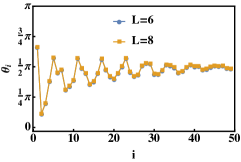
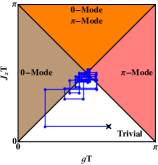
In the last example, $Z_{3}$ clock model (10), we consider $O_{0}=(\sigma_{1}+\sigma_{1}^{\dagger})/\sqrt{2}$ with $T=2$, $J=e^{i\phi}$, $h=\epsilon+i2\pi/(3\sqrt{3})$. The $Z_{3}$ clock model has an edge mode completely localized on the first site for $\epsilon=0$, where it shows period tripled dynamics, and is closely related to the decoupled edge Majorana in the TFIM for $g=0$ [31, 35]. As one moves away from $\epsilon=0$, the existence of the edge mode depends on the complex phase $\phi$ of $J$ [31, 35, 36]. In Fig. 3, we present two setups: (i) long-lived, period tripled edge mode at $\phi=\pi/2$, $\epsilon=0.1$ (top panels). (ii) short-lived, period tripled edge mode at $\phi=0$, $\epsilon=0.001$. We numerically compute the autocorrelation at three consecutive times, $n,n+1,n+2$, where $n$ equally slices the time in the logarithmic-scale and $n=1\ \text{mod}\ 3$. The upper (lower) envelope corresponds to $n+2(n,n+1)$[30]. The Krylov angles show qualitatively different behavior than the first model $U_{1}$. In setup (i), the Krylov angles approach $\pi/2$ in the bulk, even though the autocorrelation has not decayed. This is different from the chaotic cases in Fig. 2 where a Krylov angle of $\pi/2$ implied a decaying autocorrelation. In addition, for the clock model, the trajectory in the phase diagram starts from the trivial phase and approaches the center with a pattern that leads to the period tripling. In contrast to (i), in setup (ii), the trajectory of Krylov angles starts from the trivial phase but does not approach the center of the phase diagram. For both cases $K_{\rm ITFIM}$ truncated to $N=50$, fails to describe the autocorrelation at late-times indicating that the clock model requires more Krylov angles to faithfully capture the late time dynamics.

Conclusion.—We showed that the stroboscopic dynamics of any Hermitian operator under any Floquet unitary in any spatial dimension in Krylov space, is identical to the dynamics of the edge operator of a Floquet ITFIM in one spatial dimension. The details of the operator and the Floquet unitary determine the precise values of the inhomogeneous couplings of the ITFIM. The latter is a non-interacting model that can be written in terms of Majorana bilinears. Thus, this mapping allows one to leverage methods from single-particle quantum mechanics to the study of operator dynamics of an interacting quantum problem. We presented applications involving interacting Floquet spin $1/2$ chains [30] and the $Z_{3}$ clock model, where the latter hosts period-tripled edge modes. The operator dynamics shows certain universal features captured by how the Krylov parameters vary in the topological phase diagram of the non-interacting model. This universality allowed us to capture the dynamics by an efficient truncation in Krylov space. Future directions would involve further exploration of the $Z_{3}$ clock model and models in spatial dimensions $d>1$, as well as the study of other metrics such as operator entanglement.

Acknowledgments.—This work was supported by the US Department of Energy, Office of Science, Basic Energy Sciences, under Award No. DE-SC0010821. HCY acknowledges support of the NYU IT High Performance Computing resources, services, and staff expertise.

References

- Vishwanath and Müller [2008] V. Vishwanath and G. Müller, The Recursion Method: Applications to Many-Body Dynamics, Springer, New York (2008).
- Parker et al. [2019] D. E. Parker, X. Cao, A. Avdoshkin, T. Scaffidi, and E. Altman, A universal operator growth hypothesis, Phys. Rev. X 9, 041017 (2019).
- Rabinovici et al. [2021] E. Rabinovici, A. Sánchez-Garrido, R. Shir, and J. Sonner, Operator complexity: a journey to the edge of krylov space, Journal of High Energy Physics 2021, 1 (2021).
- Balasubramanian et al. [2022] V. Balasubramanian, P. Caputa, J. M. Magan, and Q. Wu, Quantum chaos and the complexity of spread of states, Phys. Rev. D 106, 046007 (2022).
- Caputa and Liu [2022] P. Caputa and S. Liu, Quantum complexity and topological phases of matter, Phys. Rev. B 106, 195125 (2022).
- Liu et al. [2023] C. Liu, H. Tang, and H. Zhai, Krylov complexity in open quantum systems, Phys. Rev. Res. 5, 033085 (2023).
- Yates et al. [2020a] D. J. Yates, A. G. Abanov, and A. Mitra, Dynamics of almost strong edge modes in spin chains away from integrability, Phys. Rev. B 102, 195419 (2020a).
- Yates et al. [2020b] D. J. Yates, A. G. Abanov, and A. Mitra, Lifetime of almost strong edge-mode operators in one-dimensional, interacting, symmetry protected topological phases, Phys. Rev. Lett. 124, 206803 (2020b).
- Yeh et al. [2023a] H.-C. Yeh, G. Cardoso, L. Korneev, D. Sels, A. G. Abanov, and A. Mitra, Slowly decaying zero mode in a weakly nonintegrable boundary impurity model, Phys. Rev. B 108, 165143 (2023a).
- Yates and Mitra [2021] D. J. Yates and A. Mitra, Strong and almost strong modes of floquet spin chains in krylov subspaces, Phys. Rev. B 104, 195121 (2021).
- Yates et al. [2022] D. Yates, A. Abanov, and A. Mitra, Long-lived period-doubled edge modes of interacting and disorder-free floquet spin chains, Communications Physics 5, 10.1038/s42005-022-00818-1 (2022).
- Suchsland et al. [2023] P. Suchsland, R. Moessner, and P. W. Claeys, Krylov complexity and trotter transitions in unitary circuit dynamics, arXiv preprint arXiv:2308.03851 (2023).
- Harper et al. [2020] F. Harper, R. Roy, M. S. Rudner, and S. Sondhi, Topology and broken symmetry in floquet systems, Annual Review of Condensed Matter Physics 11, 345 (2020).
- Oka and Kitamura [2019] T. Oka and S. Kitamura, Floquet engineering of quantum materials, Annual Review of Condensed Matter Physics 10, 387 (2019).
- Jiang et al. [2011] L. Jiang, T. Kitagawa, J. Alicea, A. R. Akhmerov, D. Pekker, G. Refael, J. I. Cirac, E. Demler, M. D. Lukin, and P. Zoller, Majorana fermions in equilibrium and in driven cold-atom quantum wires, Phys. Rev. Lett. 106, 220402 (2011).
- Rudner et al. [2013] M. S. Rudner, N. H. Lindner, E. Berg, and M. Levin, Anomalous edge states and the bulk-edge correspondence for periodically driven two-dimensional systems, Phys. Rev. X 3, 031005 (2013).
- Thakurathi et al. [2013a] M. Thakurathi, A. A. Patel, D. Sen, and A. Dutta, Floquet generation of majorana end modes and topological invariants, Phys. Rev. B 88, 155133 (2013a).
- Asbóth et al. [2014] J. K. Asbóth, B. Tarasinski, and P. Delplace, Chiral symmetry and bulk-boundary correspondence in periodically driven one-dimensional systems, Phys. Rev. B 90, 125143 (2014).
- Khemani et al. [2016] V. Khemani, A. Lazarides, R. Moessner, and S. L. Sondhi, Phase structure of driven quantum systems, Phys. Rev. Lett. 116, 250401 (2016).
- Else and Nayak [2016] D. V. Else and C. Nayak, Classification of topological phases in periodically driven interacting systems, Phys. Rev. B 93, 201103 (2016).
- Roy and Harper [2016] R. Roy and F. Harper, Abelian floquet symmetry-protected topological phases in one dimension, Phys. Rev. B 94, 125105 (2016).
- Po et al. [2016] H. C. Po, L. Fidkowski, T. Morimoto, A. C. Potter, and A. Vishwanath, Chiral Floquet phases of many-body localized bosons, Phys. Rev. X 6, 041070 (2016).
- Potter and Morimoto [2017] A. C. Potter and T. Morimoto, Dynamically enriched topological orders in driven two-dimensional systems, Phys. Rev. B 95, 155126 (2017).
- Morimoto et al. [2017] T. Morimoto, H. C. Po, and A. Vishwanath, Floquet topological phases protected by time glide symmetry, Phys. Rev. B 95, 195155 (2017).
- Fidkowski et al. [2019] L. Fidkowski, H. C. Po, A. C. Potter, and A. Vishwanath, Interacting invariants for Floquet phases of fermions in two dimensions, Phys. Rev. B 99, 085115 (2019).
- Yates et al. [2019] D. J. Yates, F. H. L. Essler, and A. Mitra, Almost strong () edge modes in clean interacting one-dimensional floquet systems, Phys. Rev. B 99, 205419 (2019).
- Thakurathi et al. [2013b] M. Thakurathi, A. A. Patel, D. Sen, and A. Dutta, Floquet generation of majorana end modes and topological invariants, Phys. Rev. B 88, 155133 (2013b).
- Yeh et al. [2023b] H.-C. Yeh, A. Rosch, and A. Mitra, Decay rates of almost strong modes in floquet spin chains beyond fermi’s golden rule, Phys. Rev. B 108, 075112 (2023b).
- Arnoldi [1951] W. E. Arnoldi, The principle of minimized iterations in the solution of the matrix eigenvalue problem, Quarterly of applied mathematics 9, 17 (1951).
- [30] See Supplemental Material.
- Sreejith et al. [2016] G. J. Sreejith, A. Lazarides, and R. Moessner, Parafermion chain with floquet edge modes, Phys. Rev. B 94, 045127 (2016).
- Kemp et al. [2017] J. Kemp, N. Y. Yao, C. R. Laumann, and P. Fendley, Long coherence times for edge spins, Journal of Statistical Mechanics: Theory and Experiment 2017, 063105 (2017).
- Else et al. [2017] D. V. Else, P. Fendley, J. Kemp, and C. Nayak, Prethermal strong zero modes and topological qubits, Phys. Rev. X 7, 041062 (2017).
- Kemp et al. [2020] J. Kemp, N. Y. Yao, and C. R. Laumann, Symmetry-enhanced boundary qubits at infinite temperature, Phys. Rev. Lett. 125, 200506 (2020).
- Fendley [2012] P. Fendley, Parafermionic edge zero modes in zn-invariant spin chains, Journal of Statistical Mechanics: Theory and Experiment 2012, P11020 (2012).
- Jermyn et al. [2014] A. S. Jermyn, R. S. K. Mong, J. Alicea, and P. Fendley, Stability of zero modes in parafermion chains, Phys. Rev. B 90, 165106 (2014).