The finite width of anyons changes their braiding signature

Abstract

Anyons are particles intermediate between fermions and bosons, characterized by a nontrivial exchange phase, yielding remarkable braiding statistics. Recent experiments have shown that anyonic braiding has observable consequences on edge transport in the fractional quantum Hall effect (FQHE). Here, we study transport signatures of anyonic braiding when the anyons have a finite temporal width. We show that the width of the anyons, even extremely small, can have a tremendous impact on transport properties and braiding signatures. In particular, we find that taking the finite width into account allows us to explain recent experimental results on FQHE at filling factor $2/5$ [Ruelle et al., Phys. Rev. X 13, 011031 (2023)]. Our work shows that the finite width of anyons crucially influences setups involving anyonic braiding, especially for composite fractions where the exchange phase is larger than $\pi/2$.

Anyons are particles intermediate between bosons and fermions, characterized by fractional exchange statistics [1, 2, 3]. These are proposed to occur in two spatial dimensions, and have found a solid experimental footing in the fractional quantum Hall effect (FQHE) [4, 5]. Fundamental interest and potential technological applications [6] have fuelled intense activity leading to several theoretical proposals to detect anyonic statistics in FQHE [7, 8, 9, 10, 11, 12, 13, 14, 15]. Only recently, experiments were able to detect anyonic statistics in the FQHE in the simplest filling fraction of $1/3$ [16, 17, 18, 19] as well as in the more complicated fraction of $2/5$ [20, 21, 22].

Transport-based experiments on FQHE edges have been successful in quantitatively extracting anyonic statistics by measuring current correlations. In contrast to spatial braiding as in the Fabry-Perot geometries, the physical mechanism at play here is time-domain braiding [23]. In the latter, anyons emitted from a source quantum point contact (QPC) form a braiding loop in time with anyon pairs excited at a QPC in FQHE. The braiding loop in time is due to the interference between two different time-ordered processes [24, 25].

Experiments are well captured by the theoretical formalism for $\nu=1/3$ FQHE where the exchange phase is $\pi/3$ [26]. However, experimental results at $\nu=2/5$, where theory predicts an exchange phase of $3\pi/5$, strongly differ from the theoretical predictions, even for a quantity as essential as the sign of the tunneling current. The multi-edge structure of $\nu=2/5$ FQHE suggests the influence of inter-edge interactions, tunneling of multiple quasiparticles at the QPC, or edge reconstruction, among others, as a possible source of the observed deviation from theoretical predictions. However, none of these candidates seem to explain the observed sign of tunneling current.

In existing calculations, the natural assumption is to neglect the temporal width of anyons. Indeed, while anyonic excitations always have a nonzero extension in the time domain, it is usually deemed negligible based on physical considerations, as it is typically much smaller than the average spacing between successive anyons, and the thermal timescale of the system. In this Letter, we show that the finite width of the anyons, even small, significantly affects their short-time braiding signatures, which is then reflected on the transport properties of the system, in particular for composite fractions of the FQHE where the exchange phase is larger than $\pi/2$. Beyond the specific system that we consider, our results show that the finite extension of anyons is an essential ingredient for a correct description of setups involving anyonic braiding.

Time-domain braiding:– We first review the basics of time-domain anyonic braiding [23, 15, 24, 27]. Consider the geometry of Fig. 1, showing a Hall bar in the FQHE with chiral edge states, equipped with a QPC operating in the weak tunneling regime, where tunneling of quasiparticles between the edges can occur. For the system at equilibrium, at all times, spontaneous processes where a quasiparticle-quasihole (qp-qh) pair is created at the QPC do exist, leading to zero net current due to electron-hole symmetry. However, when a single quasiparticle (qp) on the upper edge impinges on the QPC, there is a nontrivial interference between the process where the qp-qh pair is created before, and the one where it is created after the arrival of the single qp. The interference of these two processes leads to a braiding loop in time domain, with an overall coefficient $1-e^{2i\theta}$, where $\theta$ is the exchange phase between two qps. For fermions and bosons, the overall contribution is zero, as $\theta=\pi\mbox{ or }0$, and the tunneling current is only due to direct tunneling of the incoming qp through the QPC. For anyons however, the cancellation is only partial due to their nontrivial braiding statistics, with for example $\theta=\pi/3$ for anyonic quasiparticles in $\nu=1/3$ FQHE. It has been shown that this anyonic exchange dominantly contributes to physically measurable quantities at the QPC such as the average tunneling current, current cross-correlations and auto-correlations [24, 25]. In this work, we consider the impact of the finite width of the incoming qp on the anyonic exchange process, and its consequences on the tranport properties.

Model:– We consider a Hall bar in the FQHE with chiral edge states, equipped with a QPC where tunneling between the edge states can occur (see Fig. 1). For simplicity, each edge is described as a single mode Laughlin chiral Luttinger liquid. As shown in SM [28], this can capture exactly the physics of complex composite fractions like $\nu=2/5$ by adapting the values of the parameters (see the discussion of Eq. (3)). Up and down edge states are described in the total Hamiltonian as $H_{0u/d}=\frac{v_{F}}{4\pi}\int dx(\partial_{x}\phi^{u/d})^{2}$, where $\phi^{u/d}$ denotes the bosonic mode on the upper/lower edge, $v_{F}>0$ is the propagation velocity of the bosonic mode. The bosonic modes satisfy equal-time commutation relations $\left[\phi^{u/d}(x),\phi^{u/d}(y)\right]=\pm i\pi{Sign}(x-y)$. The edge hosts anyonic quasiparticles of charge $e^{*}=\nu e$, described by the operator $\psi\sim e^{i\sqrt{\nu}\phi}$. The QPC is placed in the weak backscattering regime, causing tunneling of anyonic qps between the two edges. The corresponding tunneling Hamiltonian is $H_{T}(t)=\Gamma\left[A(t)+A^{\dagger}(t)\right]$, where $A(t)=e^{i\sqrt{\nu}(\phi^{u}(0,t)-\phi^{d}(0,t))}$ and $\Gamma$ is the tunneling amplitude. Similarly, the current flowing from edge $u$ to $d$ is given by $I_{T}(t)=ie^{*}\Gamma\left[A^{\dagger}(t)-A(t)\right]$.

Current due to a single qp:– We first consider the current created by a single anyonic qp on the upper edge incident on the QPC. Crucially, this qp is taken to have a finite temporal extension, which can be modeled by adding a finite-width solitonic excitation on the bosonic edge modes [26, 29]

$$\phi^{u}\longrightarrow\phi^{u}+2\sqrt{\lambda}\left[\tan^{-1}\left(\frac{t-t_{0}}{t_{w}}\right)+\frac{\pi}{2}\right]$$ (1)

where $t_{w}$ denotes the width of the qp, whose center reaches the QPC at $t=t_{0}$ and $\pi\lambda$ is the phase due to the exchange of two qps. The current at the QPC due to this qp can be expressed, to leading order in $\Gamma$, using the Keldysh formalism as [30]

$$\left<I_{T}(t)\right>=-\frac{i}{2}\int dt^{\prime}\sum_{\eta\eta^{\prime}}\eta^{\prime}\left\langle\left\{T_{K}~{}I_{T}(t^{\eta})H_{T}(t^{\prime\eta^{\prime}})\right\}\right\rangle$$ (2)

where $\eta,\eta^{\prime}$ denote the Keldysh contour labels, and $T_{K}$ denotes time ordering on the Keldysh contour. It takes the form [28]

$$\left<I_{T}(t)\right>=2ie^{*}\Gamma^{2}\int_{-\infty}^{t}dt^{\prime}\left(e^{2\delta\mathcal{G}(t-t^{\prime})}-e^{2\delta\mathcal{G}(t^{\prime}-t)}\right)$$

$$\times\sin\Bigg{\{}2\lambda\left[\tan^{-1}\left(\frac{t-t_{0}}{t_{w}}\right)-\tan^{-1}\left(\frac{t^{\prime}-t_{0}}{t_{w}}\right)\right]\Bigg{\}}$$ (3)

where $\mathcal{G}(t)=\left<T\phi(t)\phi(0)\right>$ is the bosonic Green’s function

$$\mathcal{G}(t)=\ln\left(\frac{\sinh(i\pi k_{B}T\tau_{0}/\hbar)}{\sinh[\pi k_{B}T(t-i\tau_{0})/\hbar]}\right).$$ (4)

Here $\tau_{0}$ is the short-time cutoff, $T$ is the temperature, and $\delta$ is the scaling dimension of the qp tunneling across the QPC. For the Laughlin case, one simply has $\lambda=\delta=\nu$. For a composite fraction with several edge modes, the values $\lambda$ and $\delta$ can be adjusted to describe the physics of the associated qp. For example, for FQHE with filling factor $\nu=2/5$, the $e/5$ qps can be addressed simply by taking $\lambda=\delta=3/5$, and $e^{*}=e/5$, in Eq. (3). 

The incoming qp wavepacket in Eq. (1) is assumed to have a Lorentzian profile (similar expressions can be written for other shapes). Due to the finite width of the qp wavepacket, its braiding phase is smeared out in time, and it contributes only partially at a given time in the QPC, which can significantly affect the tunneling current as illustrated in Fig. 1(b). For $t_{w}\to 0$, the sine in Eq. (3) reduces to $\theta(t-t_{0})\theta(t_{0}-t^{\prime})\sin(2\pi\lambda)$, where $\theta$ is the Heaviside step function, the current then reduces to a slowly decaying function of time, with a characteristic timescale set by the temperature, $t_{\text{Th}}=\hbar/(k_{B}T)$ [31].

   

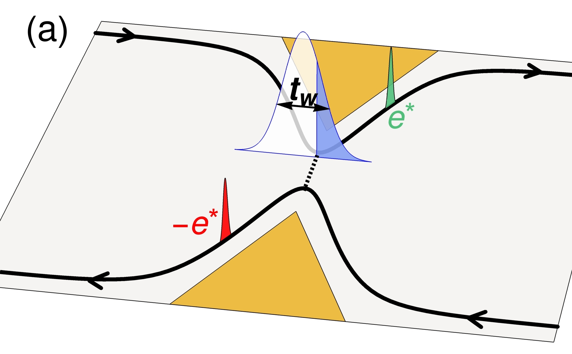
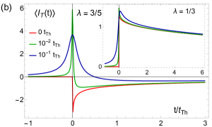
Figure 1: (a) Idealized geometry of a FQHE bar with a QPC, showing an extended quasiparticle (qp) impinging on the QPC on the upper edge (in blue/white). A tunneling current through the QPC is created by the anyonic exchange between the qp and the qp-quasihole pairs (green-red) excited at the QPC. Due to its finite temporal width ($t_{w}$), the qp contributes only partially to braiding at time $t$ at the QPC, as indicated by the blue part of the qp. (b) Tunneling current at the QPC, in units of $I_{0}=\Gamma^{2}T(\pi T\tau_{0})^{2\delta-1}$, due to a single incoming qp as a function of time (Eq. (3)) for $\lambda=\delta=3/5$, and for different qp widths ($t_{w}=0,0.01,0.1$ in units of $t_{Th}=\hbar/k_{B}T$). The center of the qp hits the QPC at $t=0$. As the width is increased one can see that the current shifts from negative to positive values. Inset: same figure for $\lambda=\delta=1/3$, showing that the effect of the qp width is not significant for $\lambda<1/2$.

We show the tunneling current as a function of time for $\lambda=3/5$ in Fig. 1(b) for different values of the width $t_{w}$ of the incoming qp. This value of $\lambda$, together with the $\delta=3/5$ we use here, corresponds to the canonical models of qp in the $2/5$ FQHE [32]. For $t_{w}=0$, the tunneling current is strictly negative, as $\sin(2\pi\times 3/5)<0$. As soon as the qp has a finite width, the current becomes positive, on a time interval around $t_{0}$ which becomes wider as $t_{w}$ is increased. Importantly, even if $\delta$ is adjusted, the qualitative behavior of the currents remains largely unchanged, as long as $\lambda>1/2$ (not shown). This behavior is in complete contrast to that at $\lambda=1/3$ (which corresponds to the usual Laughlin $\nu=1/3$ case). Here, the current due to a qp of zero width is positive. However, endowing the qp with a finite width does not significantly impact the current, as shown in the inset of Fig. 1, for parameters $\delta=1/3$. Again, the qualitative behaviour is robust against change of parameters, as long as $\lambda<1/2$.

Poissonian stream of qps:- Having detailed the behavior of the current produced by a single incoming qp, we now consider that a random Poissonian stream of qps is incident on the QPC, leading to an average current $I_{u/d}$ on the upper/lower edge. This corresponds to the situation of Ref. 16 where upstream QPCs in the tunneling regime are used as the sources of the qp streams.

In the single particle case, there were two physical time scales characterizing the system: the thermal time $t_{Th}=\hbar/(k_{B}T)$ and, $t_{w}$, the temporal width of the qp. A stream of qps introduces another important time scale: the average temporal spacing between successive qps, given by the inverse of the incoming current on the QPC, $t_{s}=e^{*}/I_{+}$, where $I_{\pm}=I_{u}\pm I_{d}$.

Choosing to normalize all times with $t_{s}$, the stream of incoming qps on the QPC can be modelled by modifying the bosonic fields as

$$\phi^{u/d}\longrightarrow\phi^{u/d}+2\sqrt{\lambda}\sum_{k}\left[\tan^{-1}\left(\frac{(t-t^{u/d}_{k})/t_{s}}{\tau_{w}}\right)+\frac{\pi}{2}\right]$$ (5)

where $t^{u/d}_{k}$ denotes the time at which the $k-$th qp on the $u/d$ edge hits the QPC, and these times follow a Poissonian distribution. Moreover, we have defined the scaled width of qps, $\tau_{w}=t_{w}/t_{s}$. Using the expression of current in Eq. (2), the average tunneling current at the QPC is [28]

$$\left\langle I_{T}\right\rangle =2ie^{*}\Gamma^{2}\int_{0}^{\infty}\!\!\!dt~{}\;\;\frac{\text{sin}\left[x\,\text{Im}f(t,\lambda,\tau_{w})\right]}{\text{exp}\left[\text{Re}f(t,\lambda,\tau_{w})\right]}$$

$$\times\left(e^{2\delta\mathcal{G}(t)}-e^{2\delta\mathcal{G}(-t)}\right)$$ (6)

where we have performed a Poisonnian average over the times $t_{k}^{u/d}$, and $x=I_{-}/I_{+}$ is the asymmetry of the incoming currents. $f(t,\lambda,\tau_{w})$ is the phase accumulated as finite-width qps pass the QPC, and is given by

$$f(t,\lambda,\tau_{w})=\int_{-\infty}^{\infty}\!\!\!du\;\Bigg{\{}1- \mbox{exp}\bigg{(}-2i\lambda\bigg{[}\tan^{-1}\left(\frac{t/t_{s}-u}{\tau_{w}}\right)$$

$$+\tan^{-1}\left(\frac{u}{\tau_{w}}\right)\bigg{]}\bigg{)}\Bigg{\}}.$$ (7)

Here, the integration over $u=t_{0}/t_{s}$ is essential as due to their finite width, the qps start affecting the QPC even before their center hits the QPC. We emphasize that Eq. (7) gives the phase accumulated due to braiding of the Poissonian stream of finite-width qps with qp-qh pairs at the QPC. This is readily seen by taking $t_{w}\to 0$, giving $f(t,\lambda,\tau_{w})\to t/t_{s}(1-e^{-2i\pi\lambda})$, which is the phase due to a stream of zero-width qps [26].

We plot the imaginary part of the finite-width phase $f(t,\lambda,\tau_{w})$ as a function of time in Fig. 2, for $\lambda=3/5$ and different values of the scaled width $\tau_{w}$. For $\tau_{w}=0$, the imaginary part of the phase is simply linear in $t$, with a negative slope equal to $\sin(2\pi\lambda)$. As soon as the qps have a finite width, we find a dramatic change occurring close to $t=0$: $\mbox{Im}f(t,\lambda,\tau_{w})$ is initially positive, and takes a finite amount of time (set by $\tau_{w}$) to become negative and eventually recover the same negative slope. This behavior is reminiscent of the behavior of the current due to a single qp shown in Fig. 1. The inset of Fig. 2 shows the imaginary part of the phase for $\lambda=1/3$. There, we see a linear behavior with a positive slope for $\tau_{w}=0$, which is only marginally affected when $\tau_{w}$ is non-zero. Note that the real part of the phase, which also enters Eq. (6), mostly contributes to the integral at short times. However, it does not vary significantly with $\tau_{w}$ for any $\lambda$, and is thus not shown here.

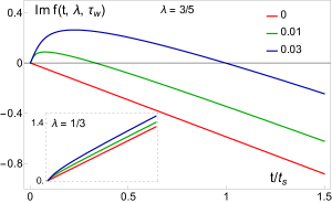
Figure 2: Imaginary part of the finite-width phase as a function of time for $\lambda=3/5$, for scaled width $\tau_{w}=0,0.01,0.03$. It is equal to $\sin(2\pi*3/5)(t/t_{s})$ for $\tau_{w}=0$, but as soon as $\tau_{w}$ is finite, the imaginary phase is positive close to $t=0$, and it takes a finite time to recover the linear behavior with a negative slope. Inset: same curves for $\lambda=1/3$, showing that for $\lambda<1/2$ a finite width does not significantly change the phase.

Hence, close to $t=0$, the effective phase experienced by the qps tunneling across the QPC is quite different from the full phase of the qp. As the rest of the integrand is peaked close to $t=0$, a sizeable contribution to the tunneling current comes from the $t\simeq 0$ region. We find that this results in an average positive tunneling current for $\lambda=3/5$, as opposed to a negative average tunneling current seen for delta-width qps. This is shown in Fig. 3(a) where the mean current $\langle I_{T}\rangle$ is plotted as a function of the scaled width $\tau_{w}$ for different values of the asymmetry $x$ of the incoming currents. One readily sees that $\langle I_{T}\rangle$ grows from negative to positive as $\tau_{w}$ is increased. For Lorentzian qp wavepackets, $\langle I_{T}\rangle$ changes sign at $\tau_{w}\sim 0.003$; for other shapes of finite width qps (not shown), the qualitative behavior is the same.

We now examine the consequence of the finite width of the incoming qps on the experimentally measured $P$ factor [28, 26], which is a generalized Fano factor for the cross-correlations of the output currents:

$$P(x=I_{-}/I_{+})=\frac{\left<\delta I_{u}\delta I_{d}\right>}{~{}~{}e^{*}I_{+}\frac{\partial\left<I_{T}\right>}{\partial I_{-}}\Big{|}_{I_{-}=0}}$$ (8)

where $\left<\delta I_{u}\delta I_{d}\right>$ denotes the current cross-correlations. The $P$ factor was measured in recent experiments [16, 20, 21] to extract anyonic statistics in FQHE. For $\nu=1/3$ FQHE, the experiments find an excellent agreement with the theory of Ref. 26 where the incoming qps are assumed to have zero width. On the other hand, for $\nu=2/5$, the experiments are in strong disagreement with the theoretical calculations, as the $P$ factor is predicted to be positive and quite large (close to 6), while the experiments measure negative values of the order of $-1$.

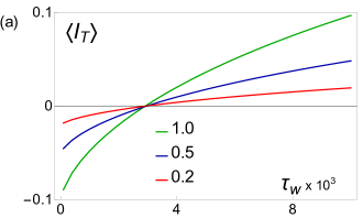
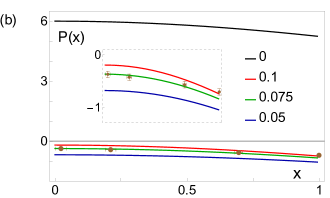
Figure 3: (a) Tunneling current $\langle I_{T}\rangle$ at the QPC due to a stream of Poissonian qp plotted as a function of scaled width $\tau_{w}$, for different values of current asymmetry: $x=0.2,0.5,1$. For very small $\tau_{w}$, $\langle I_{T}\rangle$ is negative. As the width is increased, it becomes positive at $\tau_{w}\sim 0.003$. (b) Generalized Fano factor $P(x)$ of Eq. (8) plotted as a function of the current asymmetry $x$ for different values of scaled width: $\tau_{w}=0,0.05,0.075,0.1$, Experimental data from Ref. 20 are shown as brown points with error bars. For $\tau_{w}=0$, $P(x)$ is in contradiction even with the sign of the experimentally measured values. As $\tau_{w}$ is increased, the theoretical curves become more compatible with the experimental data. The inset zooms into the region close to the experimental data points, where $\tau_{w}\sim 0.075$ agrees well with the experiments. Curves on both panels were obtained in the small temperature regime, comparable to the experimental value.

We plot the $P$ factor for $\nu=2/5$ FQHE ($\lambda=3/5,\delta=3/5$) in Fig. 3(b) for different values of the scaled width $\tau_{w}$. Experimental data points from Ref. 20 are shown in brown. The black curve denotes the predictions of Ref. 26 where $\tau_{w}=0$, and is in complete disagreement with the experimental data. With a non-zero $\tau_{w}$, the curves have now negative values, getting closer to the experimental data. The inset zooms into the region around the data points; we find that $\tau_{w}\sim 0.075$ agrees relatively well with the experiments.

The scaled width $\tau_{w}$ is proportional to the transparency $\mathcal{T}$ of the source QPCs. Indeed the applied voltage $V$ before a source QPC can be seen as a regular stream of incoming excitations whose spacing is equal to their width ($\sim 1/V$). As a fraction $\mathcal{T}$ only of these excitations is transmitted, it gives a scaled width $\tau_{w}\sim\mathcal{T}$. The value $\tau_{w}\sim 0.075$ that we find to get a reasonable agreement with the experimental results for the $P$ factor is thus compatible with the transparencies $\mathcal{T}$ used experimentally (typically $\mathcal{T}\sim 0.1$). A detailed comparison with experimental results, including the effect of varying the transparency $\mathcal{T}$ [18], and considering different shapes for the excitations, will be the subject of future work.

In conclusion, we have studied anyonic braiding signatures in edge transport of the FQHE accounting for the anyons’ finite temporal width. For a single qp incident on the QPC, the sign of the tunneling current changes due the finite width when the exchange phase $\pi\lambda>\pi/2$. For a random stream of qps incident on the QPC, relevant to the anyon collider experiment, the finite-width of the qps changes the sign of the effective braiding phase seen at the QPC for $\pi\lambda>\pi/2$. This allows us to explain quantitatively recent experiments on $\nu=2/5$ FQHE. Our conclusions are robust against variation of the scaling dimension, which is typically non-universal.

This work naturally leads to several possible extensions. Given the crucial impact of the finite width of incoming anyons, it might be interesting to study the consequences of the finite extent of the QPC [33, 34, 35]. The impact of Coulomb interaction inside the QPC could also be important for a complete description of the system. Finally, accounting for the finite width may be important in other architectures involving anyons including flying qubits [36], Fabry-Perot, and Mach-Zehnder interferometry [37], and even in different physical platforms hosting anyons such as spin liquids [38, 39, 40, 41].

Supplemental material

I Chiral Luttinger Liquid Theory of Quantum Hall Edges

In this section, we review the basics of bosonic theory of a general Abelian quantum Hall edge, and we show its application to the case of the filling factor $\nu=2/5$. The FQHE edges are modeled as chiral Luttinger liquids with a general Abelian quantum Hall edge being described by the action [42, 43]

$$S=\frac{1}{4\pi}\int dxdt\sum_{i=1}^{N}\left[-\chi_{i}\partial_{x}\phi_{i}\partial_{t}\phi_{i}-v_{i}(\partial_{x}\phi_{i})^{2}\right]$$ (S1)

where $\phi_{i}$ denote the bosonic modes on the edge, $v_{i}>0$ denote the propagation velocity of $i-$th bosonic mode, and $\chi_{i}=\pm 1$ denote their chiralities, with $i\in\{1,\dots,N\}$. The bosonic fields satisfy commutation relations given by

$$\left[\phi_{i}(x,t),\phi_{j}(x^{\prime},t^{\prime})\right]=i\pi\delta_{ij}{Sign}(X_{i}-X^{\prime}_{j})$$ (S2)

where $X_{i}=-\chi_{i}x+t$. The charge density $\rho$ and the conserved current $J$ on the edge are given by

$$\begin{split}\rho&=\frac{1}{2\pi}\sum_{i}q_{i}\partial_{x}\phi_{i}\\ J&=-\frac{1}{2\pi}\sum_{i}q_{i}\partial_{t}\phi_{i}\end{split}$$ (S3)

where $q_{i}^{2}*e^{2}/h$ is the conductance of the $i$-th bosonic mode, $e$ is the electronic charge, and $h$ the Planck’s constant. The conductance is related to the bulk filling fraction $\nu$ of the FQHE liquid via

$$\sum_{i}\chi_{i}q_{i}^{2}=\nu$$ (S4)

The edge hosts quasiparticle (qp) operators of the form

$$\psi_{\bf{g}}\sim e^{i\textbf{g}.\bm{\phi}}$$ (S5)

where vectors with $N$ components are denoted in bold, and $\textbf{A}.\textbf{B}\equiv\sum_{i}\chi_{i}A_{i}B_{i}$.

The spectrum of quasiparticle operators allowed in a given edge theory can be found in the following manner. First, we find a set of $N$ electron operators $\psi_{\bf{e_{\alpha}}}\sim e^{i{\bf{e_{\alpha}}}.\bm{\phi}}$ on the edge by demanding satisfying the following relations expected of an electronic excitation

$$\{\psi_{\bf{e_{\alpha}}}(x,t),\psi_{\bf{e_{\alpha}}}(x^{\prime},t)\} = 0,$$

$$\psi_{\bf{e_{\alpha}}}(x,t)\psi_{\bf{e_{\beta}}}(x^{\prime},t)\pm\psi_{\bf{e_{\beta}}}(x^{\prime},t),\psi_{\bf{e_{\alpha}}}(x,t) = 0,$$

$$\left[J^{0}(x,t),\psi_{\bf{e_{\alpha}}}(x^{\prime},t)\right] = \delta(x-x^{\prime})\psi_{\bf{e_{\alpha}}}(x,t).$$

Each set of $N$ electron operators defines a topological class of the quantum Hall system, which can be parametrized by the $K$ matrix

$$K_{\alpha\beta}=\bf{e}_{\alpha}\cdot\bf{e}_{\beta}$$ (S7)

Then all the allowed quasiparticle operators $\psi_{\bf{g}}\sim e^{i\textbf{g}.\bm{\phi}}$ are found by demanding that they commute or anti-commute with the electron operators

$$\psi_{\bf{g}}(x,t)\psi_{\bf{e_{\alpha}}}(x^{\prime},t)\pm\psi_{\bf{g}}(x^{\prime},t),\psi_{\bf{e_{\alpha}}}(x,t) = 0$$ (S8)

For tunneling of quasiparticles at a QPC, within a low energy approximation, the quasiparticles with the lowest scaling dimension have the highest tunneling probability. Hence, the ones with higher scaling dimensions are usually ignored, as done in this work. We emphasize that the parameters $N$, $\bf{q}$, and $\bf{\chi}$ here are phenomenological, with the values chosen below being motivated by experimental observations.

Having calculated the quasiparticle operators in a given edge theory, their relevant properties are given as follows. The charge of $\psi_{\bf{g}}$ is given by

$$q_{\bf{g}}={\bf{g}}.{\bf{q}}~{}e$$ (S9)

the scaling dimension is given by

$$\delta_{\bf{g}}=\sum_{i}g_{i}^{2}$$ (S10)

while the mutual exchange statistics of two different quasiparticle types $\psi_{\bf{g_{1}}}$ and $\psi_{\bf{g_{2}}}$ is given by

$$\theta_{\bf{g_{1}}\bf{g_{2}}}\ \equiv\pi\lambda_{\bf{g_{1}}\bf{g_{2}}}=\pi\;\bf{g_{1}}.\bf{g_{2}}$$ (S11)

Laughlin states

Laughlin states are observed for the FQHE at filling factor $\nu=1/(2m+1)$ (with $m$ and integer). The edge theory is described by a single Luttinger liquid ($N=1$), with $\bf{q}=(\sqrt{\nu})$, and $\bf{g}=(\sqrt{\nu})$. This gives for the electron operator, $\bf{e}=(1/\sqrt{\nu})$ and hence a trivial K-matrix, $(1/\nu)$. This recovers the usual results: the quasiparticle operator is given by $\psi_{\bf{g}}\sim e^{i\sqrt{\nu}\phi}$, quasiparticle charge is $q_{\bf{g}}=\nu e$, the exchange statistics is $\theta_{\bf{gg}}=\pi\nu$, and finally the scaling dimension is $\delta_{\bf{g}}=\nu$.

$\bm{\nu=2/5}$

Theoretically describing the $\nu=2/5$ FQHE state requires two chiral Luttinger liquids on the edge ($N=2$) which is consistent with experiments. Moreover, experiments see two edge modes with conductances $1/3$ and $1/15$, giving us ${\bf{q}}=(\sqrt{1/3},\sqrt{1/15})$. Both modes propagate in the same direction, hence ${\bf{\chi}=(+1,+1)}$. This choice of $\bf{q}$ and $\bf{\chi}$ satisfies Eq.(S4) and give us for the electron operators

$$\begin{split}{\bf{e_{1}}}&=\left(-2/\sqrt{3},-\sqrt{5/3}\right)\\ {\bf{e_{2}}}&=\left(-\sqrt{3},0\right)\end{split}$$ (S12)

and hence the K-matrix

$$K=\begin{pmatrix}3&2\\ 2&3\end{pmatrix}$$ (S13)

From these, it can then be shown that there exist two quasiparticles of the lowest scaling dimension, having charge $e/5$ and are given by $e^{i{\bf{g_{1}}.\bm{\phi}}}$ and $e^{i{\bf{g_{2}}.\bm{\phi}}}$, where

$$\begin{split}{\bf{g_{1}}}&=\left(0,\sqrt{3/5}\right)\\ {\bf{g_{2}}}&=\left(\sqrt{1/3},-2/\sqrt{15}\right)\end{split}$$ (S14)

Both of these charge $e/5$ quasiparticles have the same scaling dimension $\delta_{\bf{g_{1}}}=\delta_{\bf{g_{2}}}=3/5$. Their exchange statistics is given by $\theta_{\bf{g_{1}}\bf{g_{1}}}=\theta_{\bf{g_{2}}\bf{g_{2}}}=\theta_{\bf{g_{1}}\bf{g_{2}}}=3\pi/5$.

Since all the relevant quantities: charge, scaling dimension and exchange statistics are same for both $\psi_{\bf{g_{1}}}$ and $\psi_{\bf{g_{2}}}$, the features of the multiple chiral Luttinger liquid model can be captured simply by using a single chiral Luttinger liquid model with $e^{*}=e/5$, $\delta=3/5$, and $\theta=3\pi/5$, as done in the main text. In general, such a simplification can always be done for all fully chiral quantum Hall edges (${\bm{\chi}}=(+1,\dots,+1)$).

II Current due to single quasiparticle: General Abelian quantum Hall edge

In this section, we calculate the tunneling current due to a single quasiparticle incident on the Quantum Point Contact, using the general theory shown in the previous section. For simplicity, we a make the simplifying assumption of a single type of quasiparticle tunneling across the QPC (generalization is straightforward). The tunneling Hamiltonian of the QPC is given by

$$H_{T}(t)=\Gamma\left(e^{i\bf{g_{1}}.\bm{\phi^{u}}-i\bf{g_{1}}.\bm{\phi^{d}}}+hc\right)$$ (S15)

while the tunneling current from the upper edge to the lower edge is

$$I_{T}(t)=iq_{\bf{g_{1}}}\Gamma\left(e^{i\bf{g_{1}}.\bm{\phi^{u}}-i\bf{g_{1}}.\bm{\phi^{d}}}-hc\right)$$ (S16)

A single quasiparticle flows on the upper edge, hitting the QPC at time $t_{0}$. This process is modelled by augmenting the bosonic field $\bm{\phi^{u}}$ with a solitonic excitation

$$\phi^{u}_{i}\longrightarrow\phi_{i}^{u}+2\pi g_{2i}\left[\frac{1}{\pi}\tan^{-1}\left(\frac{t-t_{0}}{t_{w}}\right)+\frac{1}{2}\right]$$ (S17)

where we have assumed for the sake of illustration, that the quasiparticle tunneling across the QPC, and the one impinging on the QPC are of different types. The tunneling current in the QPC can be expressed within the Keldysh formalism as

$$\left<I_{T}(t)\right>=-\frac{i}{2}\int dt^{\prime}\sum_{\eta\eta^{\prime}}\eta^{\prime}\left\langle\left\{T_{K}~{}I_{T}(t^{\eta})H_{T}(t^{\prime\eta^{\prime}})\right\}\right\rangle$$ (S18)

where $\eta,\eta^{\prime}$ denote the Keldysh contour labels, and $T_{K}$ denotes time ordering on the Keldysh contour. We plug in the tunneling Hamiltonian and tunneling current operators

$$\left<I_{T}(t)\right>=\frac{q_{\bf{g_{1}}}\Gamma^{2}}{2}\int dt^{\prime}~{}\sum_{\epsilon\eta\eta^{\prime}}\epsilon\eta^{\prime}\left\langle\left\{T_{K}~{}\left[e^{i{\bf{g_{1}}}.\bm{\phi}^{u}(t^{\eta})-i{\bf{g_{1}}}.\bm{\phi}^{d}(t^{\eta})}\right]^{\epsilon}\left[e^{i{\bf{g_{1}}}.\bm{\phi}^{u}(t^{\prime\eta^{\prime}})-i{\bf{g_{1}}}.\bm{\phi}^{d}(t^{\prime\eta^{\prime}})}\right]^{-\epsilon}\right\}\right\rangle$$ (S19)

where the sum over $\epsilon$ exists to account for the both terms in Eqs. (S15) and (S16). We can further expand this as

$$\begin{split}\left<I_{T}(t)\right>=\frac{q_{\bf{g_{1}}}\Gamma^{2}}{2}\int dt^{\prime}~{}\sum_{\epsilon\eta\eta^{\prime}}\epsilon\eta^{\prime}&\prod_{j}\left<\left\{T_{K}~{}e^{i\epsilon g_{1j}\phi_{j}^{u}(t^{\eta})}e^{-i\epsilon g_{1j}\phi_{j}^{u}(t^{\prime\eta^{\prime}})}\right\}\right>\left<\left\{T_{K}~{}e^{-i\epsilon g_{1j}\phi_{j}^{d}(t^{\eta})}e^{i\epsilon g_{1j}\phi_{j}^{d}(t^{\prime\eta^{\prime}})}\right\}\right>\\ &\exp\left\{2\epsilon g_{1j}g_{2j}\left[\tan^{-1}\left(\frac{t-t_{0}}{t_{w}}\right)-\tan^{-1}\left(\frac{t^{\prime}-t_{0}}{t_{w}}\right)\right]\right\}\end{split}$$ (S20)

Using now the identity,

$$\left<\left\{T_{K}~{}e^{i\epsilon g_{1j}\phi_{j}^{u/d}(t^{\eta})}e^{-i\epsilon g_{1j}\phi_{j}^{u/d}(t^{\prime\eta^{\prime}})}\right\}\right>=e^{g_{1j}^{2}\mathcal{G}_{j}^{\eta\eta^{\prime}}(t-t^{\prime})}$$ (S21)

where $\mathcal{G}^{\eta\eta^{\prime}}(t)$ denotes the components of the Keldysh Greens function, and summing over $\epsilon$, we get

$$\left<I_{T}(t)\right>=2iq_{\bf{g_{1}}}\Gamma^{2}\int dt^{\prime}~{}\sum_{\eta\eta^{\prime}}\eta^{\prime}\prod_{j}e^{2g_{1j}^{2}\mathcal{G}_{j}^{\eta\eta^{\prime}}(t-t^{\prime})}~{}\sin\Bigg{\{}2\sum_{j}g_{1j}g_{2j}\left[\tan^{-1}\left(\frac{t-t_{0}}{t_{w}}\right)-\tan^{-1}\left(\frac{t^{\prime}-t_{0}}{t_{w}}\right)\right]\Bigg{\}}$$ (S22)

Summing now over the Keldysh contour indices and using the relations between different components of the Keldysh Green’s function [30], the current takes the form

$$\begin{split}&\left<I_{T}(t)\right>=2iq_{\bf{g_{1}}}\Gamma^{2}\int_{-\infty}^{t}dt^{\prime}\left(e^{\sum_{j}2g_{1j}^{2}\mathcal{G}_{j}(t-t^{\prime})}-e^{\sum_{j}2g_{1j}^{2}\mathcal{G}_{j}(t^{\prime}-t)}\right)\sin\Bigg{\{}2\sum_{j}g_{1j}g_{2j}\left[\tan^{-1}\left(\frac{t-t_{0}}{t_{w}}\right)-\tan^{-1}\left(\frac{t^{\prime}-t_{0}}{t_{w}}\right)\right]\Bigg{\}}\end{split}$$ (S23)

where the summation inside the sine includes only the bosonic modes flowing towards the QPC, and

$$\mathcal{G}_{j}(t)\equiv\mathcal{G}^{-+}_{j}(t)=\ln\left(\frac{\sinh(i\pi k_{B}T\tau_{0j}/\hbar)}{\sinh[\pi k_{B}T(t-i\tau_{0j})/\hbar]}\right)$$ (S24)

where $\tau_{0j}$ is the cutoff corresponding to the $j-$th bosonic mode. We then have

$$\sum_{j}g_{j}^{2}=\delta_{\bf{g}}$$ (S25)

and for fully chiral edges ,

$$\sum_{j}g_{1j}g_{2j}\equiv{\bf{g_{1}}.\bf{g_{2}}}=\lambda_{\bf{g_{1}g_{2}}}\equiv\theta_{g_{1}g_{2}}/\pi$$ (S26)

representing the exchange phase of the quasiparticles $\psi_{\bf{g_{1}}}$ and $\psi_{\bf{g_{2}}}$. Finally, in the limit $\tau_{0j}\rightarrow 0$

$$\mathcal{G}_{j}(t)\equiv\mathcal{G}(t)=\ln\left(\frac{\sinh(i\pi k_{B}T\tau_{0}/\hbar)}{\sinh[\pi k_{B}T(t-i\tau_{0})/\hbar]}\right)$$ (S27)

for all $j$, where $\tau_{0}$ is smaller than the smallest $\tau_{0j}$. With this, we can write for fully chiral edges

$$\left<I_{T}(t)\right>=2iq_{\bf{g_{1}}}\Gamma^{2}\int_{-\infty}^{t}dt^{\prime}\left(e^{2\delta_{\bf{g_{1}}}\mathcal{G}(t-t^{\prime})}-e^{2\delta_{\bf{g_{1}}}\mathcal{G}(t^{\prime}-t)}\right)\sin\Bigg{\{}2\lambda_{\bf{g_{1}g_{2}}}\left[\tan^{-1}\left(\frac{t-t_{0}}{t_{w}}\right)-\tan^{-1}\left(\frac{t^{\prime}-t_{0}}{t_{w}}\right)\right]\Bigg{\}}$$ (S28)

From the above one can see that the current through the QPC for an edge theory with multiple bosonic modes can be simply captured using a single chiral Luttinger liquid expression, by appropriate choice of the parameters $q_{\bf{g_{1}}}$, $\delta_{\bf{g_{1}}}$ and $\lambda_{\bf{g_{1}g_{2}}}$, as done in the main text.

III Theory of the Anyon Collider

We outline here the theory of the anyon collider, following Ref. [26]. The geometry of the anyon collider comprises three QPCs. The QPCs on the left and right are biased with a voltage $V$, and are placed in the weak-backscattering regime. These QPCs emit fractional quasiparticles on the opposite edges, which then travel downstream toward the central QPC. The left and right QPCs, called source QPCs henceforth, act as sources of random stream of quasiparticles for the central QPC. The stream of incoming quasiparticles can be modeled by augmenting the bosonic fields with solitons as

$$\phi_{i}^{u/d}\longrightarrow\phi_{i}^{u/d}+2\pi g_{i}\sum_{k}\left[\frac{1}{\pi}\tan^{-1}\left(\frac{t-t^{u/d}_{k}}{t_{w}}\right)+\frac{1}{2}\right]$$ (S29)

where the times $t_{k}^{u/d}$ denote the time at which the $k$-th quasiparticle on the upper/lower edge hits the central QPC, and these times follow a Poissonian distribution. We have assumed here that a single type of quasiparticle is emitted on the edges from the source QPCs. The Poissonian stream of quasiparticles gives rise to an average input current $I_{u/d}$ on the upper/lower edge. The average tunneling current at the central QPC can be expressed with the Keldysh formalism as

$$\left<I_{T}\right>=-\frac{i}{2}\int dt^{\prime}\sum_{\eta\eta^{\prime}}\eta^{\prime}\left\langle\left\{T_{K}~{}I_{T}(t^{\eta})H_{T}(t^{\prime\eta^{\prime}})\right\}\right\rangle$$ (S30)

where $\eta,\eta^{\prime}$ denote the Keldysh contour labels, and $T_{K}$ denotes time ordering on the Keldysh contour. The tunneling Hamiltonian $H_{T}(t)$ is given by

$$H_{T}(t)=\Gamma\left(e^{i\bf{g}.\bm{\phi_{u}}}e^{-i\bf{g}.\bm{\phi_{d}}}+hc\right)$$ (S31)

where we have assumed that a single type of quasiparticle tunnels across the central QPC. The tunneling current can then be shown to take the form [26, 29]

$$\left<I_{T}\right> =2ie^{*}\Gamma^{2}\int_{0}^{\infty}\!\!\!dt~{}\;\;\frac{\text{sin}\left[x\text{Im}f(t,\lambda,\tau_{w})\right]}{\text{exp}\left[\text{Re}f(t,\lambda,\tau_{w})\right]}\left(e^{2\delta\mathcal{G}(t)}-e^{2\delta\mathcal{G}(-t)}\right)$$ (S32)

where $x=I_{+}/I_{-}$, $I_{\pm}=I_{u}\pm I_{d}$, and the phase accumulated due to finite width quasiparticles is given by

$$f(t,\lambda,\tau_{w})=\int_{-\infty}^{\infty}\!\!\!du\;\Bigg{\{}1- \mbox{exp}\bigg{(}-2i\lambda\Big{[}\tan^{-1}\left(\frac{t/t_{s}-u}{\tau_{w}}\right)-\tan^{-1}\left(\frac{0-u}{\tau_{w}}\right)\Big{]}\bigg{)}\Bigg{\}}$$ (S33)

The tunneling noise at the QPC can be expressed as

$$\left<S_{T}\right>=\int dt^{\prime}\sum_{\eta\eta^{\prime}}\eta^{\prime}\left\langle\left\{T_{K}~{}I_{T}(t^{\eta})I_{T}(t^{\prime\eta^{\prime}})\right\}\right\rangle$$ (S34)

which after some manipulations gives us

$$\left<S_{T}\right> =e^{2*}\Gamma^{2}\int_{0}^{\infty}\!\!\!dt~{}\;\;\frac{\text{cos}\left[x\text{Im}f(t,\lambda,\tau_{w})\right]}{\text{exp}\left[\text{Re}f(t,\lambda,\tau_{w})\right]}\left(e^{2\delta\mathcal{G}(t)}+e^{2\delta\mathcal{G}(-t)}\right)$$ (S35)

In the limit $t_{w}\longrightarrow 0$, these assume the form in Ref. [26]

$$\left<I_{T}\right>=2ie^{*}\Gamma^{2}\int_{0}^{\infty}\!\!\!dt~{}\;\;\frac{\text{sin}\left[\frac{I_{-}}{e^{*}}t\sin(2\pi\lambda)\right]}{\text{exp}\left[\frac{I_{+}}{e^{*}}t(1-\cos(2\pi\lambda))\right]}\left(e^{2\delta\mathcal{G}(t)}-e^{2\delta\mathcal{G}(-t)}\right)$$ (S36)

$$\left<S_{T}\right>=e^{2*}\Gamma^{2}\int_{0}^{\infty}\!\!\!dt~{}\;\;\frac{\text{cos}\left[\frac{I_{-}}{e^{*}}t\sin(2\pi\lambda)\right]}{\text{exp}\left[\frac{I_{+}}{e^{*}}t(1-\cos(2\pi\lambda))\right]}\left(e^{2\delta\mathcal{G}(t)}+e^{2\delta\mathcal{G}(-t)}\right)$$ (S37)

The current cross-correlations, which are accessible experimentally, are related to the tunneling noise and tunneling current via a fluctuation-dissipation relation

$$\left<\delta I_{u}\delta I_{d}\right> =-\left<S_{T}\right>+e^{*}\left(I_{+}\frac{\partial}{\partial I_{-}}+I_{-}\frac{\partial}{\partial I_{+}}\right)\left<I_{T}\right>$$ (S38)

Finally, we define a generalized Fano factor, dividing the cross-correlations by the differential transmission of the QPC

$$P(x=I_{-}/I_{+})=\frac{\left<\delta I_{u}\delta I_{d}\right>}{~{}~{}e^{*}I_{+}\frac{\partial\left<I_{T}\right>}{\partial I_{-}}\Big{|}_{I_{-}=0}}$$ (S39)