Spherical Collapse Approach for Non-standard Cold Dark Matter Models and Enhanced Early Galaxy Formation in JWST

Abstract

We examine the impact of two alternative dark matter models that possess distinct non-zero equations of state, one constant and the other time-dependent, on the nonlinear regime using the spherical collapse approach. Specifically, we compare these models to standard cold dark matter (CDM) by analyzing their influence on the linear density threshold for nonrelativistic component collapse and virial overdensity. Additionally, we explore the number count of collapsed objects, or dark matter halos, which is analogous to the number count of galaxy clusters. Finally, in light of recent discoveries by the James Webb Space Telescope (JWST), which indicate the potential for more efficient early galaxy formation at higher redshifts, we have been investigating how alternative dark matter assumptions can enhance structure formation efficiency during the early times.

1 Introduction and motivation

The need for a non-baryonic matter component has been established at the galactic scale since the early 1930s by observations such as the rotation curve of the galaxy [1, 2] and, on the cosmological scale, by observations such as gravitational lensing, large-scale structure (LSS) and cosmic microwave background(CMB) [3]. However, the origin and nature of dark matter remain a mystery and an open problem despite many years of research in astrophysics and particle physics.

In the present work, we study the nonlinear evolution of matter density perturbations for two alternative dynamical dark matter models. Gunn and Gott  [4], in 1972, introduced in a seminal paper the spherical collapse model (SCM) for the first time. The SCM is a semi-analytical and simple approach to studying the nonlinear evolution of the growth of overdensities in sub-horizon regions. The scales of the SCM are much smaller than the Hubble horizon and the velocities are non-relativistic in this approach. The overdense region is assumed to be spherically symmetric and to have a uniform density which is higher than the background density of dark matter.

At early times, due to the small growth of perturbations, the linear theory of perturbations could describe the evolution of spherical overdensities properly. Due to self-gravity, we expect that the spherical overdense patch expands at a slower rate compared to the Hubble flow expansion. Therefore, the overdense sphere becomes denser and denser than the background. Consequently, at a certain redshift which is known as the turnaround redshift, $z_{{}_{\rm ta}}$, the overdense region reaches a maximum radius and starts to compress afterward, and eventually collapses and completely decouples from the background expansion. After $z_{{}_{\rm ta}}$, the overdense spherical region collapses under its self-gravity to reach the steady state virial radius at a certain redshift $z_{{}_{\rm vir}}$ [5, 6].

The procedure for the evolution of spherical perturbations, starting from initial fluctuations at early times and ending due to the viralization procedure, strongly depends on the evolution of the background cosmology. In the framework of standard General Relativity (GR), several independent investigations have been prompted into the subject of SCM [7]. The formalism has been thoroughly analyzed within the context of scalar-tensor and modified gravities [8]. However, we note that there are other complex numerical methods to study the nonlinear evolution of cosmic perturbations and the formation of large-scale structures in the Universe, such as the N-body simulations in which the codes require longer running times [9].

In [10], it was discussed how the change in the DM characteristic parameters, such as the equation of state, $w$, and the effective sound speed, $c^{2}_{{}_{s}}$, affect the linear overdensity threshold for collapse, $\delta_{{}_{c}}$, and the virial overdensity, $\Delta_{{}_{\rm vir}}$. They showed that a relatively high value of the sound speed is required to change the evolution of $\delta_{{}_{c}}$ between the GDM and the CDM standard model, i.e. $c^{2}_{{}_{s}}\sim 10^{-4}$, but $w$ has a much stronger effect than that induced by the sound speed and it becomes more pronounced for $\delta_{{}_{c}}$ than $\Delta_{{}_{\rm vir}}$ for values around $w\sim 10^{-3}$. This is because $w$ modifies the background expansion history, while $c^{2}_{{}_{s}}$ only affects the perturbations. In this work, in addition to the model reviewed in [10], we investigate the nonlinear evolution of matter perturbations, focusing on an alternative cold dark matter model with a dynamical equation of state and predicting the abundance of virialized halos in this model.

Recently, the JWST Cosmic Evolution Early Release Science (CEERS) program derived the cumulative stellar mass density at $7<z<10$ based on 14 galaxy candidates with masses in the range $\sim 10^{9}-10^{10}M_{\odot}$ using the 1-5 $\mu$m coverage data [11]. This release of early JWST observational data has challenged the current theory of galaxy formation under the $\Lambda$CDM model [12, 13, 14]. Specifically, the authors of [12] have expressed this to be a serious tension with the standard galaxy formation theory. They recognized six galaxies with stellar masses $M_{\star}=10^{10}\sim 10^{11}h^{-1}M_{\odot}$ at $7.4\leq z\leq 9.1$. Their comoving cumulative stellar mass density is about 20 times higher at $z\sim 8$ and about three orders of magnitude higher at $z\sim 9$ than the prediction from the star formation theory in standard $\Lambda$CDM cosmology, which is based on previous observations. Although the huge abundance excess may be due to issues of galaxy selection, measurements of galaxy stellar mass and redshift, dust extinction, and sample variance, if future spectroscopic observation (for example through the follow-up observation by the JWST/NIRSpec) confirms this difference, it will be an important challenge to the $\Lambda$CDM model. Various solutions to solve this tension have been proposed so far, such as the rapidly accelerating primordial black holes [15], the primordial non-Gaussianity in the initial conditions of cosmological perturbations [16], the Fuzzy Dark Matter [17], the cosmic string [18], and a gradual transition in the stellar initial mass function [19]. In our investigation, we will try to address the difference by assuming alternative dark matter models.

This paper is structured as follows: in Sec. 2, we briefly introduce the equation of state of the considered dark matter models and describe the evolution of the Hubble flow in these models. In Sec. 3, the basic equations for the evolution of density perturbations in the linear and nonlinear regimes are presented. In Sec. 4, first we investigate the linear and nonlinear density perturbations for the considered models to obtain the values of the cosmic parameters using the latest cosmological data. After that, in Sec. 5, we study nonlinear structure formation. In Sec. 6, we compute the predicted mass function and the number count of halos using the Press-Schechter formalism. Subsequently, in Sec. 7, we investigate the comoving stellar mass density contained within galaxies more massive than $M_{\star}$ and compare our findings with the JWST observations. Finally, in Sec. 8, we summarize our conclusions.

2 Background dynamics

A flat, homogeneous, and isotropic Universe is described by the Friedmann-Lemaitre-Robertson-Walker (FLRW) metric

$$ds^{2}=-dt^{2}+a^{2}(t)(dr^{2}+r^{2}d\theta^{2}+r^{2}\sin^{2}\theta d\phi^{2})\,,$$ (2.1)

where $a(t)$ is the scale factor at the cosmic time $t$. In the framework of general relativity, we can obtain the Friedmann background dynamics equations by inserting Eq. (2.1) into the Einstein field equations, which yields

$$H^{2}=\frac{8\pi G}{3}\,\Sigma\rho_{{}_{j}}\,,$$ (2.2)

$$\dot{H}=-4\pi G\,\Sigma(\rho_{{}_{j}}+p_{{}_{j}})\,,$$ (2.3)

where $H\equiv\dot{a}/a$ is the Hubble parameter, and $\rho_{{}_{j}}$ and $p_{{}_{j}}$, respectively, represent the mean energy density and mean pressure of each component $j$. We assume that the material content of the Universe is composed of four components: radiation, baryons, dark matter, and dark energy, and all of them are described by ideal fluids with the equation of state $w_{{}_{j}}=p_{{}_{j}}/\rho_{{}_{j}}$. The energy densities of these components fulfill the following conservation equation

$$\dot{\rho}_{{}_{j}}+3H(\rho_{{}_{j}}+p_{{}_{j}})=0\,.$$ (2.4)

The radiation component (photons($\gamma$)+relativistic neutrinos) will be denoted by the sub-index “R” and it is characterized by a state parameter $w_{{}_{R}}=1/3$. We set $\Omega_{{}_{R,0}}=\Omega_{{}_{\gamma,0}}(1+0.2271N_{{}_{\rm eff}})$ that $N_{\rm eff}$, and the effective extra relativistic degrees of freedom put 3.046 in agreement with the standard model prediction [20] and $\Omega_{{}_{\gamma,0}}=2.469\times 10^{-5}h^{-2}$, where the reduced Hubble constant $h$ is defined as usual according to $H_{{}_{0}}\equiv 100h\,\mathrm{km\,s^{-1}Mpc^{-1}}$. The baryon component will be denoted by the sub-index “B”, and since it is a pressureless component, so $w_{{}_{B}}=0$. The dark energy component is considered as a cosmological constant, $\Lambda$, with a constant equation of state (EoS) parameter $w_{{}_{\Lambda}}=-1$. Lastly, the dark matter component will be denoted by the sub-index “DM”. It is considered in this study as the following divisions:

• For the first model, we consider dark matter as a non-luminous, dark component of matter that must be non-relativistic or cold, similar to the standard model of cosmology $\Lambda$CDM. It means that cold dark matter is pressureless matter fluid, so $w_{{}_{DM}}=0$. For a flat Universe through the Friedmann equation, we can write the Hubble parameter as

  $$H^{2}(a)=H_{{}_{0}}^{2}\left(\Omega_{{}_{R,0}}a^{-4}+\Omega_{{}_{B,0}}a^{-3}+\Omega_{{}_{DM,0}}a^{-3}+\Omega_{\Lambda}\right)\,.$$ (2.5)

• For the dynamical dark matter model, we consider the simplest model, that dark matter has a constant non-zero equation of state, so we can write the Hubble parameter using the continuity equation $\dot{\rho}=-3H(1+w)\rho$ as

  $$H^{2}(a)=H_{{}_{0}}^{2}\left(\Omega_{{}_{R,0}}a^{-4}+\Omega_{{}_{B,0}}a^{-3}+\Omega_{{}_{DM,0}}a^{-3(1+w)}+\Omega_{{}_{\Lambda}}\right)\,.$$ (2.6)

• To explore whether the dark matter equation of state evolves, a simple approach is to consider the dark matter EoS as a function of redshift. Specifically, we consider the so-called Chevallier-Polarski-Linder (CPL) parametrization $w(a)=w_{{}_{0}}+w_{{}_{1}}(1-a)$, where the parameter $w_{{}_{1}}$ describes the rate of evolution of dark matter [21]. So we obtain the Hubble parameter as

  $$H^{2}(a)=H_{{}_{0}}^{2}\left(\Omega_{{}_{R,0}}a^{-4}+\Omega_{{}_{B,0}}a^{-3}+\Omega_{{}_{DM,0}}a^{-3(1+w_{0}+w_{1})}e^{3w_{1}(a-1)}+\Omega_{{}_{\Lambda}}\right)\,.$$ (2.7)

  This case reduces to cold dark matter when $w_{{}_{0}}=w_{{}_{1}}=0$.

In all the models, due to the flatness of the Universe, we have

$$\Omega_{{}_{\Lambda}}=1-\Omega_{{}_{R,0}}-\Omega_{{}_{B,0}}-\Omega_{{}_{DM,0}}\,.$$ (2.8)

3 Cosmological perturbations

As we know, the large-scale structures in the Universe provide invaluable information about the nature of unknown dark components in addition to the background evolution. The primordial matter perturbations grow throughout cosmic history and their growth rate depends on the overall energy budget and the properties of the cosmic fluids.

By assuming the stress-energy tensor of a perfect fluid for each component $j$ as

$$T_{j}^{\mu\nu}=(\rho_{j}+P_{j})u^{\mu}u^{\nu}+P_{j}g^{\mu\nu}\,,$$ (3.1)

where $u^{\mu}$ is the four-velocity of each fluid. To define the density contrast between a single fluid by the relation $\delta_{j}+1=\rho_{j}/\bar{\rho}$ with the background density $\bar{\rho}$ and the three-dimensional comoving peculiar velocity $\vec{u}$. Contracting the continuity equation, $\bigtriangledown_{\mu}T^{\mu\nu}=0$, once with $\vec{u}$ and once with the projection operator $h_{\mu\alpha}=g_{\mu\alpha}+u_{\mu}u_{\alpha}$, we can derive the continuity and the Euler equations (the perturbation equations) as follows:

$$\dot{\delta}_{j}+3H(c_{s,j}^{2}-w_{j})\delta_{j}+\left[1+w_{j}+(1+c_{s,j}^{2})\delta_{j}\right]\vec{\nabla}.\vec{u}_{j}=0\,,$$ (3.2)

$$\dot{\vec{u}}_{j}+2H\vec{u}_{j}+(\vec{u}_{j}.\vec{\nabla})\vec{u}_{j}+\frac{\vec{\nabla}\phi}{a^{2}}=0\,,$$ (3.3)

where $c_{s}^{2}=\delta p/\delta\rho$ is the effective sound speed and the dot denotes the derivative with respect to the physical time. The peculiar gravitational potential is denoted by $\phi$, and it satisfies the Poisson equation obtained from the 00-component of Einstein’s field equations

$$\nabla^{2}\phi=4\pi G\Sigma\rho_{j}(1+3c^{2}_{s,j})\delta_{j}\,.$$ (3.4)

The divergence of equation 3.3 can be written as

$$\dot{\theta}_{j}+2H\theta_{j}+\frac{1}{3}\theta_{j}^{2}+\frac{\nabla^{2}\phi}{a^{2}}=0\,,$$ (3.5)

where $\theta_{j}\equiv\vec{\nabla}.\vec{u}_{j}$ and we have used $\vec{\nabla}.[(\vec{u}_{j}.\vec{\nabla})\vec{u}_{j}]=\frac{1}{3}\theta_{i}^{2}$. We can also rewrite equation 3.2 as

$$\dot{\delta}_{j}+3H(c^{2}_{s,j}-w_{j})\delta_{i}+[1+w_{j}+(1+c^{2}_{s,j})\delta_{j}]\theta_{j}=0\,.$$ (3.6)

As mentioned in the previous section, we assumed dark matter as a non-zero pressure fluid, with the EoS parameter $w$. Since we do not have an evolution equation for $\delta p$, we approximate $c_{\rm s}^{2}$ by the adiabatic sound speed $c^{2}_{{\rm ad}}=w-\frac{\dot{w}}{3H(1+w)}$. Replacing the equation (3.3) with the equation (3.2), and eliminating $\theta_{j}$ from the system of equations and introducing quantities

$$A_{j}\equiv 3H(c^{2}_{s,j}-w_{j})\qquad\&\qquad B_{j}\equiv\delta_{j}+[1+w_{j}+(1+c^{2}_{s,j})\delta_{j}]\theta_{j}\,,$$

we can obtain the following equation:

$$\ddot{\delta}_{j}+\left(2H-\frac{\dot{B}_{j}}{B_{j}}\right)(A_{j}+\dot{\delta}_{j})-\frac{1}{3}\frac{(\dot{\delta}_{j}+A_{j})^{2}}{B_{j}}-\frac{B_{j}}{a^{2}}\nabla^{2}\phi=0\,.$$ (3.7)

Since we consider dark energy as the cosmological constant and it does not change in space and time, it cannot cluster like matter, so $\delta_{\Lambda}=0$. Using the relation $\frac{d}{dt}=aH\frac{d}{da}$, equation (3.7) can be written in terms of the scale factor as

$$\delta^{\prime\prime}_{m}+A_{m}\delta^{\prime}_{m}+B_{m}\delta_{m}-\frac{3}{2a^{2}}\Omega_{m}(a)[1+w+(1+c^{2}_{s})\delta_{m}](1+3c^{2}_{s})\delta_{m}(1+\delta_{m})=C_{m}\delta^{2}_{m}+D_{m}\frac{\delta^{\prime 2}_{m}}{1+\delta_{m}}\,,$$ (3.8)

where prime denotes derivative with respect to $a$ and the coefficients are

$$A_{m}=\frac{3}{a}(1+c^{2}_{s}-w)+\frac{H^{\prime}}{H}-\frac{w^{\prime}}{1+w+(1+c^{2}_{s})\delta_{m}}\,,$$

$$B_{m}=\frac{3}{a}\left[(c^{2}_{s}-w)(\frac{2}{a}+\frac{H^{\prime}}{H})-w^{\prime}-\frac{w^{\prime}(c^{2}_{s}-w)}{1+w+(1+c^{2}_{s})\delta_{m}}\right]\,,$$

$$C_{m}=\frac{3}{a^{2}}\frac{c^{2}_{s}-w}{1+w+(1+c^{2}_{s})\delta_{m}},$$

$$D_{m}=\frac{4+3c^{2}_{s}}{3(1+w+(1+c^{2}_{s})\delta_{m})}\,.$$

As expected, in the case of cold dark matter model ($w=c^{2}_{s}=0$), equation (3.8) is reduced to the well-known differential equation

$$\delta^{\prime\prime}_{m}+\left(\frac{3}{a}+\frac{H^{\prime}}{H}\right)\delta^{\prime}_{m}-\frac{3}{2a^{2}}\Omega_{m}(a)\delta_{m}(1+\delta_{m})=\frac{4}{3}\frac{\delta^{\prime 2}_{m}}{1+\delta_{m}}\,.$$ (3.9)

In the following sections, we will solve this differential equation to find the evolution of the matter density contrast.

4 Alternative models of dark matter versus the cosmological data

Since we need the constrained values of the free parameters of the model and also the cosmological parameters, to be able to check the spherical collapse model, we will try to confine the models introduced in the previous section to the background and perturbations levels using the latest cosmological data via the Markov Chain Monte Carlo (MCMC) method. For this purpose, we implement the related equations in the publicly available numerical code CLASS (Cosmic Linear Anisotropy Solving System) [22] and using the code MONTEPYTHON-v3 [23, 24] to perform a Monte Carlo Markov chain analysis with a Metropolis-Hasting algorithm. In our analysis, we use the combinations of data points including luminosity distance of type Ia supernovas (SNIa, 1048 points from the Pantheon sample) [25], cosmic chronometers ($H(z)$, 30 points from Table 4 of [26]), measurements of the growth rate of structure weighted by a redshift-dependent normalization, $f(z)\sigma_{8}(z)$, obtained by fitting WiggleZ Survey data and SDSS-III Baryon Oscillation Spectroscopic Survey [27], and the CMB temperature and polarization angular power spectra (the high-l TT, TE, EE +low-l TT, EE+lensing data from Planck 2018) [20].

We have reported the result of our MCMC analysis for the three models in Tables 1 and 2. Also, we show 1D posterior distributions and 2D contours of the free parameters for all the models in Fig. 1. Given the Jeffreys’ scale [28], since the difference between the AIC of a given model and the CDM model is smaller than 4, we conclude that the models examined in this work and the CDM model are equally supported by the observational data.

Table 1: The best values of the free parameters obtained for the considered models.

NDM-cte	best-fit	mean$\pm\sigma$	95% lower	95% upper
$\Omega_{\mathrm{B}}$	$0.04891$	$0.04906_{-0.00079}^{+0.00079}$	$0.04701$	$0.5092$
$\Omega_{\mathrm{DM}}$	$0.2586$	$0.2596_{-0.0046}^{+0.0069}$	$0.2473$	$0.2689$
$H_{0}$	$67.93$	$67.84_{-0.54}^{+0.42}$	$66.93$	$68.93$
$S_{8}$	$0.817$	$0.818\pm 0.012$	$0.790$	$0.842$
$w_{0}$	$-0.0003626$	$-0.0004322_{-0.00043}^{+0.00033}$	$-0.001285$	$0.0005327$
NDM-CPL	best-fit	mean$\pm\sigma$	95% lower	95% upper
$\Omega{}_{B}$	$0.0481$	$0.04826_{-0.00058}^{+0.00047}$	$0.0473$	$0.04933$
$\Omega{}_{DM}$	$0.2536$	$0.256_{-0.0061}^{+0.0049}$	$0.2454$	$0.2672$
$H_{0}$	$68.39$	$68.23_{-0.4}^{+0.49}$	$67.32$	$69.09$
$S_{8}$	$0.822$	$0.826\pm 0.012$	$0.803$	$0.851$
$10^{+4}w_{0}$	$0.01738$	$0.04403^{+0.068}_{-0.046}$	$-0.113$	$0.127$
$10^{+4}w_{1}$	$0.0001436$	$0.0001399_{-0.00013}^{+0.00012}$	$-0.0001166$	$0.0004044$
CDM	best-fit	mean$\pm\sigma$	95% lower	95% upper
$\Omega{}_{B}$	$0.04836$	$0.04806_{-0.00055}^{+0.00047}$	$0.04707$	$0.04912$
$\Omega{}_{DM}$	$0.2561$	$0.2536_{-0.0062}^{+0.0049}$	$0.2427$	$0.2653$
$H_{0}$	$68.24$	$68.42_{-0.44}^{+0.5}$	$67.48$	$69.3$
$S_{8}$	$0.826$	$0.820\pm 0.012$	$0.797$	$0.843$

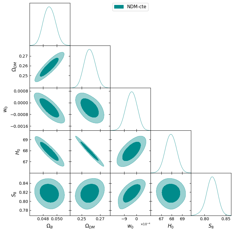
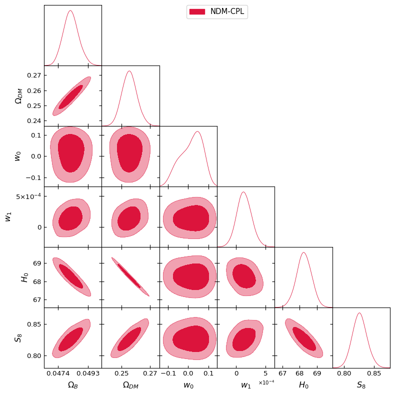
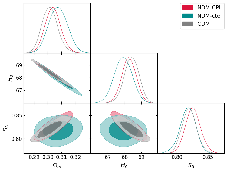
Figure 1: Reconstructed 2D posterior distribution in the considered model.

Table 2: The result of MCMC analysis for all the reviewed models in this study for the best-fit $\chi^{2}$.

	CDM	NDM-cte	NDM-CPL
$\chi^{2}_{\rm min}$	$4639.34$	$4638.00$	$4637.26$
$\rm AIC-AIC_{\rm CDM}$	$-$	$0.66$	$1.92$

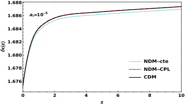
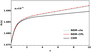
Figure 2: Critical collapse density $\delta_{c}$ as a function of redshift for different values of $a_{i}$.

5 Nonlinear perturbations

In this section, we study the nonlinear structure formation in the presence of a non-standard dark matter component. To survey the nonlinear perturbation theory and to compute the rate of formation of massive objects, the simplest (semi-) analytical tool that can provide exact nonlinear results is the spherical collapse (SC) formalism. The SC method allows for explicit computation of nonlinear dynamics that can also serve as a basis to evaluate several quantities of cosmological interest, such as the halo mass functions and the probability distributions of the density contrast [29].

Now, we calculate two main quantities of the SC formalism, the critical density contrast at collapse, $\delta_{c}$, and the viral overdensity parameter, $\Delta_{{}_{\rm vir}}$, for different dark matter scenarios. $\delta_{c}$ is defined as the value of the linear density contrast at the redshift where the nonlinear density contrast diverges. We remember that the linear overdensity $\delta_{c}$ is employed to calculate the mass function of dark matter halos in the Press-Schechter formalism and the size of the viralized halos is determined by the virial overdensity $\Delta_{\rm vir}$.

To determine $\delta_{c}$ and $\Delta_{\rm vir}$, we follow the general approach outlined in [30]. We searched for the proper initial condition, $\delta_{m,i}$, and its derivative $\delta^{\prime}_{m,i}$ to obtain highly nonlinear values of overdensities, $\delta\rightarrow\infty$, such as $\sim 10^{7}$, at a collapse redshift $z_{c}$ using Eq. (3.8). We rewrite the Eq. (3.8) in a linear regime as

$$\delta^{\prime\prime}_{m}+\left(\frac{3}{a}(1+c^{2}_{s}-w)+\frac{H^{\prime}}{H}-\frac{w^{\prime}}{1+w}\right)\delta^{\prime}_{m}-\frac{3}{2a^{2}}\Omega_{m}(a)(1+w)(1+3c^{2}_{s})\delta_{m}=0\,,$$ (5.1)

and using the obtained initial conditions, we solve the linear Eq. (5.1) to calculate the linear overdensity $\delta_{c}=\delta_{m}(z=z_{c})$. Since the initial scale factor for the numerical solution of the equations is not clear, we can consider the two cases, $a_{i}=10^{-5}$ and $a_{i}=10^{-4}$. We figured out the critical density contrast, $\delta_{c}$, as a function of redshift at the collapse. Since the fiducial value in the EdS Universe is $\delta_{c}=1.686$, we show in the graphs of Fig. 2 that for $a_{i}=10^{-5}$, we have essentially converged to the expected value of $1.686$. So in the rest of the study, we focused on $a_{i}=10^{-5}$ as the initial scale factor. We observe that in the two models, $\delta_{c}$ approaches a constant value at high enough redshifts and this value is larger than the NDM-CPL model ($\delta_{c,{}_{\rm CDM}}<\delta_{c,{}_{\rm NDM-cte}}<\delta_{c,{}_{\rm NDM-CPL}}$). This is because at high redshifts the Universe is dominated by dark matter and at lower redshifts, $\delta_{c}$ decreases and deviates from the EdS limit.

We now investigate the virialization process of dark matter halos in the context of SC formalism. The overdensity of viralized halos is defined as $\Delta_{{}_{\rm vir}}=\xi(x/y)^{3}$, where $\xi$ is the amount of overdensity at the turnaround epoch, $x$ is the scale factor normalized to turnaround scale factor ($x=a/a_{{}_{\rm ta}}$ ), and $y$ is the ratio between the virial radius and the turn-around radius ($y=R_{{}_{\rm vir}}/R_{{}_{\rm ta}}$) [31]. In the preliminary EdS cosmology, we can easily obtain $y=1/2$, $\xi\approx 5.6$, and $\Delta_{{}_{\rm vir}}=178$ at any cosmic epoch of the Universe. In Fig 3, we observe that in all the models, the turnaround overdensity $\xi$ converges to the fiducial value $\xi\approx 5.6$, which represents EdS cosmology at early times. The results of the virial overdensity $\Delta_{\rm vir}$ are presented in Fig. 4. There are lower densities of virialized halos at low redshifts in the dynamical DM and CDM models than in the EdS Universe ($\Delta_{{}_{\rm vir}}=178$). This can be interpreted as the effect of DE on the process of virialization. In fact, DE prevents more collapse and, consequently, halos viralize at a larger radius with a lower density.

At the end of this section, we remember that although these differences are small, their combined effect enters exponentially in the evaluation of the halo mass function. So, even a small difference can be amplified and lead to a noticeable difference. Hence, when the high-mass end is considered, it makes it a very reasonable probe for cosmology [10].

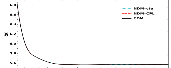
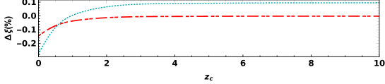
Figure 3: Evolution of $\xi$ as a function of collapse redshift, $z_{c}$, for NDM-cte and NDM-CPL models and their difference with CDM cosmology.

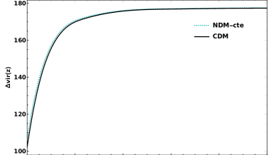
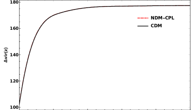
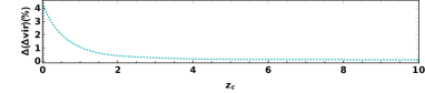
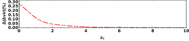
Figure 4: Evolution of the virial overdensity, $\Delta_{\rm vir}$, as a function of the collapse redshift, $z_{c}$, for the NDM-cte (left panels) and NDM-CPL (right panels) models and their difference with the CDM cosmology.

6 Halo mass function and cluster number count

As we know, the spherical collapse parameters cannot be observed directly, and so it is more convenient to evaluate the comoving number density of virialized structures with masses in a certain range. This quantity is related closely to the observations of structure formation. Therefore, in this section, we study the distribution of the number density of collapsed objects of a given mass range using a sophisticated formalism, named Press-Schechter, with the assumption of alternatives to cold dark matter. In the semi-analytic approach, there is another different mathematical formulation of halos mass, called the Sheth-Tormen formalism, which is a generalization of the Press-Schechter formalism. The mathematical formulations of the halo mass function are based on the assumption of a Gaussian distribution of the matter density field. The comoving number densities of virialized halos with masses in the range of $M$ and $M+dM$ in terms of collapse redshift $z$ is given by

$$\frac{dn(z,M)}{dM}=-\frac{\rho_{m,0}}{M}\frac{d\ln\sigma(z,M)}{dM}f(\sigma(z,M))\,,$$ (6.1)

where $\rho_{m,0}$ is present-day matter energy density and $f(\sigma)$ is called the mass function. A traditional Gaussian distribution function, $f(\sigma)$, is proposed by Press and Schechter (PS) [32] as

$$f(\sigma)=\sqrt{\frac{2}{\pi}}\frac{\delta_{c}(z)}{\sigma(z,M)}\exp\left[-\frac{\delta_{c}^{2}(z)}{2\sigma^{2}(z,M)}\right]\,,$$ (6.2)

where $\sigma$ is the root mean square of the mass fluctuations in spheres of radius $R$ containing the mass $M$ [32]. Note that function (6.2) works well in calculating the predicted number density of virialized halos with moderate mass but it fails by estimating a high abundance of low-mass structures and less abundance of high-mass objects. Hence, in this work, we use the Sheth-Torman (ST) mass function which is in better agreement with simulations at low and high mass tails and it is given by [33]

$$f(\sigma)=A\sqrt{\frac{2a}{\pi}}\left[1+\left(\frac{\sigma^{2}(z,M)}{a\delta_{c}^{2}(z)}\right)^{p}\right]\left(\frac{\delta_{c}(z)}{\sigma(z,M)}\right)\exp\left[-\frac{a\delta_{c}^{2}(z)}{2\sigma^{2}(z,M)}\right]\,.$$ (6.3)

Here, $A=0.3222$, $a=0.707$, and $p=0.3$. Note that the PS mass function is recovered in the limit $A=a\rightarrow 1$ and $p\rightarrow 0$. As we see, the quantities $\delta_{c}$ and mass variance $\sigma$ depend strongly on the cosmological model considered. The amplitude of mass fluctuation $\sigma(z,M)$ in the Gaussian density fields are expressed in terms of the growth factor ${\cal{D}}(z)=\delta(z)/\delta(0)$ as

$$\sigma(z,M)=\sigma(0,M_{8})\left(\frac{M}{M_{8}}\right)^{-\gamma/3}{\cal{D}}(z)\,,$$ (6.4)

where $M_{8}$ denotes the mass within a sphere of radius $R=8h^{-1}$Mpc and it is givin by $M_{8}=4\pi R^{3}\rho_{m0}/3$ and we take it approximately as $\sim 8\times 10^{14}\Omega_{m0}h^{-1}M_{\odot}$, where $M_{\odot}$ denotes the solar mass. In Eq. (6.4), the parameter $\gamma$ is defined as

$$\gamma=\left(0.3\Omega_{dm0}\exp[-\Omega_{b0}-\sqrt{2h}\frac{\Omega_{b0}}{\Omega_{dm0}}]h+0.2\right)\left[2.92+\frac{1}{3}\log_{10}(\frac{M}{M_{8}})\right]\,.$$ (6.5)

According to the above formulation, the number density of virialized halos above a specified mass $M$ at collapse redshift $z$ is given by

$$n(>M_{{}_{\rm halo}},z)=\int_{M_{{}_{\rm halo}}}^{\infty}\frac{dn(z,M)}{dM}dM\,.$$ (6.6)

In practice, we fix the above limit of integration as $M=10^{18}M_{\odot}h^{-1}$, as such a gigantic structure could not be observed. This quantity is of interest in galaxy observations with high redshifts.

In Fig. 5, we show the ratio of the predicted number of halos above a certain mass $M$ normalized to the CDM model for two set different cosmic redshifts: $z=0,1,2$ (low redshifts) and $z=7,9,10$ (high redshifts) in the mass range $10^{13}M_{\odot}\ll M\ll 10^{15}M_{\odot}$. As we observe in all cases, at higher redshifts, differences in halo numbers between alternative dark matter models and the CDM Universe appear even at low masses. In all the redshifts, the NDM-CPL model predicts a higher number of virialized objects compared to the NDM-cte model. Therefore, we see that the additional characteristics of the dark matter sector have a strong impact on the observables, not only on the linear evolution of perturbations but also on the nonlinear evolution of the formation of structures through the halo mass function.

The cumulative halo mass density, $\rho_{m}(>M_{\rm halo},z)$, is another closely related quantity given by

$$\rho_{m}(>M_{{}_{\rm halo}},z)=\int_{M_{{}_{\rm halo}}}^{\infty}M\frac{dn(z,M)}{dM}dM\,.$$ (6.7)

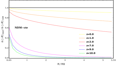
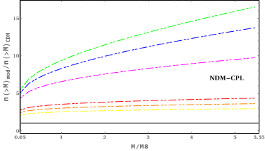
Figure 5: Ratio of the number of virialized halos above a certain mass $(>M)$ at $z=0$ until $z=10$ for the different dark matter models to the CDM cosmology. Line styles and colors are shown in the legends.

Through a straightforward assumption that the largest stellar content a halo can have is its cosmic allotment of baryons, these convert directly to upper limits on the statistics of galaxies as $M_{\star,max}=\epsilon f_{b}M_{{}_{\rm halo}}$, where $f_{b}\equiv\frac{\Omega_{b}}{\Omega_{m}}$ is the cosmic baryon fraction and $\epsilon\leq 1$ is the efficiency of converting gas into stars.

A useful quantity that we will be mostly interested in and concerns the JWST observations is the cumulative comoving mass density of stars contained in galaxies more massive than $M_{\star}$, $\rho_{\star}(>M_{\star},z)$, defined as

$$\rho_{\star}(>M_{\star},z)=\epsilon f_{b}\int_{M_{\star}/(\epsilon f_{b})}^{\infty}M\frac{dn(z,M)}{dM}dM\,.$$ (6.8)

We can use this quantity to evaluate the viability of the CDM model. In the following section, we use the potential of the JWST observations in discriminating between different DM models.

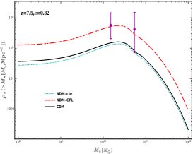
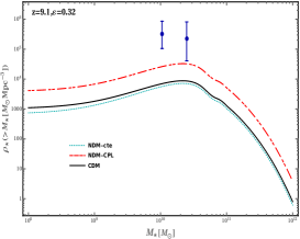
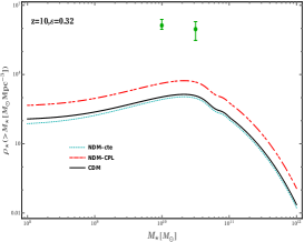
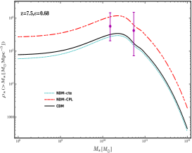
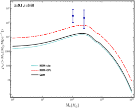
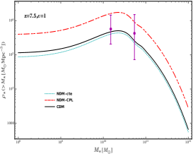
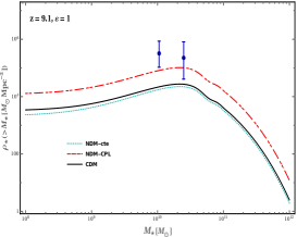
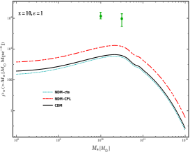
Figure 6: The comoving stellar mass density contained within galaxies more massive than $M_{\star}$ at $z=7.5$ (left panel), $z=9.1$ (middle panel), and $z=10$ (right panel) for various values of the assumed conversion efficiency $\epsilon=0.32,0.68$ and $1$ of a halo’s cosmic allotment of baryons into stars.

7 Comparison with the JWST observations

Galaxies with stellar masses up to $\sim 10^{11}M_{\odot}$ have been detected approximately one billion years after the Big Bang, up to redshift $z\sim 6$. It has been difficult to find massive galaxies at earlier times (known as the Balmer break region) since, for accurate mass estimates, they need to be redshifted to wavelengths beyond 2.5 $\mu$m. On the other hand, the study of high redshift galaxies is important since it allows us to have a deeper understanding of the formation and evolution of early galaxies and the history of cosmic reionization.

Here, we calculate the cumulative comoving stellar mass density within galaxies with stellar mass above $\rho_{\star}(>M_{\star})$ for different DM models for three redshifts probed by the analysis of JWST CEERS data: $z=7.5$, $z=9.1$, and $z=10$. In Fig. 6, we show the theoretical predictions for the comoving cumulative stellar mass density ($\rho_{\star}(>M_{\star})$) in terms of $M_{\star}$. Here, we assume three different values of the efficiency of converting gas into stars $\epsilon=0.32,0.68$, and the conservative value, $\epsilon=1$ that maximizes the stellar mass predicted by a given scenario. We find that both alternative DM models and CDM are consistent with JWST data at $z=7.5$ when the assumed conversion efficiency, $\epsilon=1$. As we see, the NDM-CPL model for all three different values of $\epsilon$ at $z=7.5$ is compatible with the JWST data. For $z=9.1$, the CDM and NDM-cte fail to explain the JWST data, but NDM-CPL with $\epsilon=1$ manages to increase the $\rho_{\star}(>M_{\star})$ up to the level claimed by JWST. But for $z=10$, as we see in the figure, we find all three theoretical models under study predict a lower value compared to the JWST observations.

So far, we have focused on the best-fit values for the parameters in the different scenarios for the DM equation of state. In the following, we try to plot $\rho_{\star}(>M_{\star})$ for different values of those parameters. In particular, we consider 10 different models (4 NDM-cte and 6 NDM-CPL models), corresponding to various arbitrary values of the parameters $w_{0}$ and $w_{1}$, for both two dark matter models. Our goal is to investigate the effect of changing the dark matter equation of state in justifying the high redshift $z=10$ observed by the JWST. For this purpose, we set the values of other free cosmological parameters to be the same in all cases as $\Omega_{m}=0.3$ and $H_{0}=70\rm kms^{-1}Mpc^{-1}$. We show the result in Fig. 7 and notice an interesting point in these plots: for smaller negative values for both models, we will have a better agreement with the observed values. So we see the theoretical predictions for $\rho_{\star}(>M_{\star})$ in the NCDM-cte model for $w=-0.05$ and in the NDM-CPL model for $w_{0}=-0.05$ and $w_{1}=0.005$ (note that at the high redshifts, the CPL EoS tends to $w_{0}+w_{1}$ ) for various values of the assumed conversion efficiency $\epsilon$ are consistent to the observational data at $z=10$. In Fig. 8, we can see that for these two cases that are in agreement with the JWST observational data, the different values of the critical density obtain smaller values than the standard model.

In our computations, we have assumed that the critical overdensity, $\delta_{c}$, is independent of the mass scale and only dependent on redshift, but since the equation of the state of alternative DM models is nonzero, it is more appropriate to consider its dependence on mass, $\delta_{c}(z,M)$, and this is left for future studies.

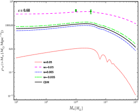
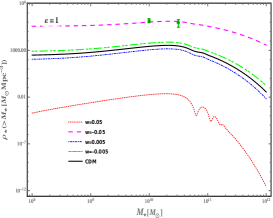
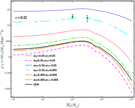
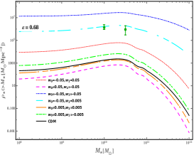
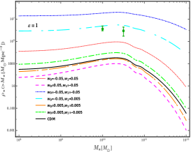
Figure 7: The comoving stellar mass density contained within galaxies more massive than $M_{\star}$ at $z=10$ for the 10 different dark matter models (4 NDM-cte and 6 NDM-CPL models) for various values of the assumed conversion efficiency $\epsilon=0.32,0.68$ and $1$ of a halo’s cosmic allotment of baryons into stars.

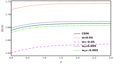
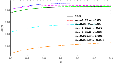
Figure 8: Evolution of the critical collapse density, $\delta_{c}$, as a function of redshift, for the different dark matter models.

8 Conclusions

In a flat FLRW Universe, we investigated the perturbations of dark matter with different non-zero equations of states in the nonlinear regime. For this purpose, we used the spherical collapse method, which is an efficient analytical approach to investigate structure formation in the nonlinear regime. In the first step, we constrained our models by using the novel cosmological data including luminosity distance of type Ia supernovas, cosmic chronometers, measurements of the growth rate of structure, and the CMB temperature and polarization angular power spectra via the Markov Chain Monte Carlo method to obtain the current values of the free and cosmological parameters to check the spherical collapse model. In the next step, we computed the spherical collapse parameters including the linear overdensity $\delta_{c}(z_{c})$, the virial overdensity $\Delta_{{}_{\rm vir}}(z_{c})$, and the overdensity at the turnaround $\xi(z_{c})$. Our results imply: (i) the linear overdensity $\delta_{c}$ at high redshifts, goes toward the expected value of $\delta_{c}=1.686$ in the EdS limit, (ii) the virial overdensity $\Delta_{{}_{\rm vir}}$ and the overdensity at the turnaround $\xi$ in initial times converge to 178 and 5.55, respectively, which are the same values corresponding to the EdS Universe as we expected given the impact of DE at high redshifts is negligible. Our results imply that $n(>M)_{\rm mod}/n(>M)_{\rm CDM}$, in the NDM-cte (NDM-CPL) model is lower (more) than the CDM results.

In the final section, we discussed that according to unexpected high stellar mass densities of massive galaxies at $7\lesssim z\lesssim 10$, found by the early JWST observations, higher star formation efficiency is expected and can have tension with the current measurements of the standard CDM model. So we investigated the comoving stellar mass density contained within galaxies more massive than $M_{\star}$. Our results show that the NDM-CPL model is consistent for all different values of $\epsilon$ up to $z=9$ for JWST data, but for higher redshifts ($z=10$), the JWST observations suggest an excess of the comoving stellar mass density above the predictions of our theoretical models.

As it is clear from the plots of Fig. 7, having dark matter with a negative equation of state parameters, $w_{1}<0$ is very important in increasing the theoretical predictions for the cumulative stellar mass density, thereby improving the agreement with the JWST results.

References

- [1] V. C. Rubin and W. K. Ford, Jr., “Rotation of the Andromeda Nebula from a Spectroscopic Survey of Emission Regions,” Astrophys. J. 159 (1970) 379–403.
- [2] V. C. Rubin, N. Thonnard, and W. K. Ford, Jr., “Rotational properties of 21 SC galaxies with a large range of luminosities and radii, from NGC 4605 /R = 4kpc/ to UGC 2885 /R = 122 kpc/,” Astrophys. J. 238 (1980) 471.
- [3] Planck Collaboration, N. Aghanim et al., “Planck 2018 results. I. Overview and the cosmological legacy of Planck,” Astron. Astrophys. 641 (2020) A1, 1807.06205.
- [4] J. E. Gunn and J. R. Gott, III, “On the Infall of Matter into Clusters of Galaxies and Some Effects on Their Evolution,” Astrophys. J. 176 (1972) 1–19.
- [5] T. Padmanabhan, Structure Formation in the Universe. Cambridge University Press, 1996.
- [6] P. Fosalba and E. Gaztanaga, “Cosmological perturbation theory and the spherical collapse model: Part 1. Gaussian initial conditions,” Mon. Not. Roy. Astron. Soc. 301 (1998) 503–523, astro-ph/9712095.
- [7] S. Basilakos, J. Bueno Sanchez, and L. Perivolaropoulos, “The spherical collapse model and cluster formation beyond the cosmology: Indications for a clustered dark energy?,” Phys. Rev. D 80 (2009) 043530.
- [8] Y. Fan, P. Wu, and H. Yu, “Spherical collapse in the extended quintessence cosmological models,” Phys. Rev. D 92 (2015), no. 8, 083529, 1510.04010.
- [9] F. Pace, J. C. Waizmann, and M. Bartelmann, “Spherical collapse model in dark energy cosmologies,” Mon. Not. Roy. Astron. Soc. 406 (2010) 1865, 1005.0233.
- [10] F. Pace, Z. Sakr, and I. Tutusaus, “Spherical collapse in Generalized Dark Matter models,” Phys. Rev. D 102 (2020), no. 4, 043512, 1912.12250.
- [11] I. Labbé, P. van Dokkum, E. Nelson, R. Bezanson, K. A. Suess, J. Leja, G. Brammer, K. Whitaker, E. Mathews, M. Stefanon, and B. Wang, “A population of red candidate massive galaxies 600 Myr after the Big Bang,” Nature 616 (Apr., 2023) 266–269, 2207.12446.
- [12] M. Boylan-Kolchin, “Stress testing CDM with high-redshift galaxy candidates,” Nature Astron. 7 (2023), no. 6, 731–735, 2208.01611.
- [13] C. A. Mason, M. Trenti, and T. Treu, “The brightest galaxies at cosmic dawn,” Mon. Not. Roy. Astron. Soc. 521 (2023), no. 1, 497–503, 2207.14808.
- [14] T. Matsumoto and B. D. Metzger, “Light-curve Model for Luminous Red Novae and Inferences about the Ejecta of Stellar Mergers,” Astrophys. J. 938 (2022), no. 1, 5, 2202.10478.
- [15] G.-W. Yuan, L. Lei, Y.-Z. Wang, B. Wang, Y.-Y. Wang, C. Chen, Z.-Q. Shen, Y.-F. Cai, and Y.-Z. Fan, “Rapidly growing primordial black holes as seeds of the massive high-redshift JWST Galaxies,” 2303.09391.
- [16] M. Biagetti, G. Franciolini, and A. Riotto, “High-redshift JWST Observations and Primordial Non-Gaussianity,” Astrophys. J. 944 (2023), no. 2, 113, 2210.04812.
- [17] Y. Gong, B. Yue, Y. Cao, and X. Chen, “Fuzzy Dark Matter as a Solution to Reconcile the Stellar Mass Density of High-z Massive Galaxies and Reionization History,” Astrophys. J. 947 (2023), no. 1, 28, 2209.13757.
- [18] H. Jiao, R. Brandenberger, and A. Refregier, “Early structure formation from cosmic string loops in light of early JWST observations,” Phys. Rev. D 108 (2023), no. 4, 043510, 2304.06429.
- [19] A. Trinca, R. Schneider, R. Valiante, L. Graziani, A. Ferrotti, K. Omukai, and S. Chon, “Exploring the nature of uv-bright galaxies detected by jwst: star formation, black hole accretion, or a non universal imf?,” 2305.04944.
- [20] Planck Collaboration, N. Aghanim et al., “Planck 2018 results. VI. Cosmological parameters,” Astron. Astrophys. 641 (2020) A6, 1807.06209. [Erratum: Astron.Astrophys. 652, C4 (2021)].
- [21] M. Chevallier and D. Polarski, “Accelerating universes with scaling dark matter,” IJMP D 10 (2001) 213–224.
- [22] J. Lesgourgues and T. Tram, “The Cosmic Linear Anisotropy Solving System (CLASS) IV: efficient implementation of non-cold relics,” JCAP 09 (2011) 032, 1104.2935.
- [23] B. Audren, J. Lesgourgues, K. Benabed, and S. Prunet, “Conservative Constraints on Early Cosmology: an illustration of the Monte Python cosmological parameter inference code,” JCAP 02 (2013) 001, 1210.7183.
- [24] T. Brinckmann and J. Lesgourgues, “MontePython 3: boosted MCMC sampler and other features,” Phys. Dark Univ. 24 (2019) 100260, 1804.07261.
- [25] Pan-STARRS1 Collaboration, D. M. Scolnic et al., “The Complete Light-curve Sample of Spectroscopically Confirmed SNe Ia from Pan-STARRS1 and Cosmological Constraints from the Combined Pantheon Sample,” Astrophys. J. 859 (2018), no. 2, 101, 1710.00845.
- [26] M. Moresco, L. Pozzetti, A. Cimatti, R. Jimenez, C. Maraston, L. Verde, D. Thomas, A. Citro, R. Tojeiro, and D. Wilkinson, “A 6% measurement of the Hubble parameter at : direct evidence of the epoch of cosmic re-acceleration,” JCAP 05 (2016) 014, 1601.01701.
- [27] BOSS Collaboration, S. Alam et al., “The clustering of galaxies in the completed SDSS-III Baryon Oscillation Spectroscopic Survey: cosmological analysis of the DR12 galaxy sample,” Mon. Not. Roy. Astron. Soc. 470 (2017), no. 3, 2617–2652, 1607.03155.
- [28] A. Bonilla Rivera and J. E. García-Farieta, “Exploring the Dark Universe: constraints on dynamical Dark Energy models from CMB, BAO and growth rate measurements,” Int. J. Mod. Phys. D28 (2019), no. 09, 1950118, 1605.01984.
- [29] P. Brax and P. Valageas, “Structure Formation in Modified Gravity Scenarios,” Phys. Rev. D 86 (2012) 063512, 1205.6583.
- [30] F. Pace, R. C. Batista, and A. Del Popolo, “Effects of shear and rotation on the spherical collapse model for clustering dark energy,” MNRAS 445 (2014) 648.
- [31] L.-M. Wang and P. J. Steinhardt, “Cluster abundance constraints on quintessence models,” Astrophys. J. 508 (1998) 483–490, astro-ph/9804015.
- [32] W. H. Press and P. Schechter, “Formation of galaxies and clusters of galaxies by selfsimilar gravitational condensation,” Astrophys. J. 187 (1974) 425–438.
- [33] R. K. Sheth and G. Tormen, “Large scale bias and the peak background split,” Mon. Not. Roy. Astron. Soc. 308 (1999) 119, astro-ph/9901122.