VSCode: General Visual Salient and Camouflaged Object Detection
with 2D Prompt Learning

Abstract

Salient object detection (SOD) and camouflaged object detection (COD) are related yet distinct binary mapping tasks. These tasks involve multiple modalities, sharing commonalities and unique cues. Existing research often employs intricate task-specific specialist models, potentially leading to redundancy and suboptimal results. We introduce VSCode, a generalist model with novel 2D prompt learning, to jointly address four SOD tasks and three COD tasks. We utilize VST as the foundation model and introduce 2D prompts within the encoder-decoder architecture to learn domain and task-specific knowledge on two separate dimensions. A prompt discrimination loss helps disentangle peculiarities to benefit model optimization. VSCode outperforms state-of-the-art methods across six tasks on 26 datasets and exhibits zero-shot generalization to unseen tasks by combining 2D prompts, such as RGB-D COD.

1 Introduction

Visual salient object detection (SOD) and camouflaged object detection (COD) are two interconnected yet unique tasks. The goal of SOD is to identify prominent objects within an image that significantly contrast with their surroundings [5]. While COD focuses on identifying objects concealed within their environment. These objects intentionally blend in by sharing structural or textural similarities with their surroundings [16]. Despite the seemingly different definitions of SOD and COD, they both belong to the realm of binary segmentation and share some vital fundamental similarities, such as objectness and structuredness.

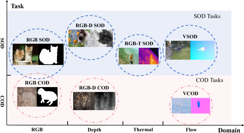
Figure 1: Relationship of SOD, COD, and multimodal tasks. Each specific task is seen as a combination of two dimensions, i.e. domain (RGB/Depth/Thermal/Flow) and task (SOD/COD).

To cater to various scenarios, both SOD and COD have given rise to several sub-tasks with different modalities, including RGB SOD [80, 119, 95], RGB COD [69, 112, 75], RGB-D SOD [120, 50, 80], RGB-D COD [104], and RGB-T SOD [89, 92, 118]. By leveraging optical flow maps, Video SOD (VSOD) [98, 52, 103] and VCOD [3, 44, 11] tasks can also be seen as a combination of two modalities. The relationship of SOD, COD, and multimodal tasks is shown in Figure 1, where each specific task can be considered as a combination of two dimensions, i.e.  domain and task. Although these multimodal tasks differ in the complementary cues they employ, these modalities share some key commonalities. For instance, depth, thermal, and optical flow maps often show obvious objectness as in RGB images.

Although previous CNN-based [80, 120, 89, 98, 69, 11] and transformer-based [62, 129] approaches have effectively addressed these tasks and achieved favorable results, they usually rely on meticulously designed models to tackle each task individually. Designing models specifically for individual tasks can be problematic since the training data of one task is typically limited. Task-specific specialist models may be overly adapted to a particular task and overfitted to specific training data distribution, which ultimately sacrifices generalization ability and results in suboptimal performance. One solution may be using more data, however, being costly and time-consuming for data annotation. To this end, joint learning a generalist model emerges as a more promising option, as it allows for the maximum use of all data and the effective learning of the commonalities of all tasks, hence significantly reducing the risk of overfitting and enhancing the generalization capability [42, 63]. However, joint learning multiple tasks is not straightforward. On one hand, simultaneously handling both commonalities and peculiarities of all tasks poses a significant challenge as the incompatibility among different tasks easily leads to a decline in performance with simple joint training [48]. On the other hand, it usually introduces additional complexity, computational costs, and parameters.

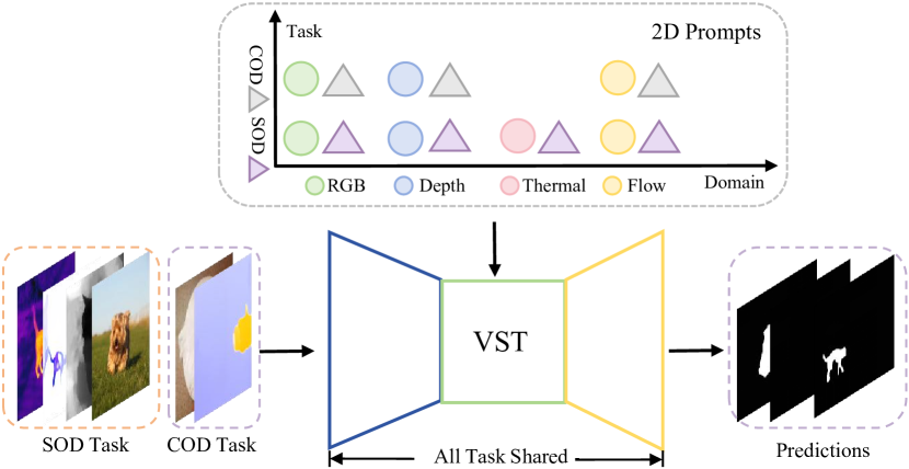
Figure 2: Overall architecture of our VSCode model. We use VST [62] as the foundation model to acquire commonalities among multimodal SOD and COD tasks. For each task, we integrate 2D prompts to aggregate peculiarities along the domain dimension and the task dimension, including four domain-specific prompts and two task-specific prompts.

In this paper, we present a general Visual Salient and Camouflaged object detection (VSCode) model which encapsulates both commonalities and peculiarities of different tasks with a simple but effective design, as illustrated in Figure 2. On one hand, we adopt VST [62] as the shared segmentation foundation model to assimilate commonalities of different tasks by leveraging its simple and pure-transformer-based architecture. On the other hand, inspired by the recent emergence of the parameter-efficient prompting technique [71, 39, 33], we propose 2D prompts to capture task peculiarities. Specifically, we decompose these peculiarities along the domain dimension and the task dimension, and consequently design domain-specific prompts and task-specific prompts to comprehend the differences among diverse domains and tasks, respectively. These 2D prompts can effectively disentangle domain and task peculiarities, making our model easily adaptable by combining them to tackle specific tasks and even unseen ones. Furthermore, we present a prompt discrimination loss to encourage the 2D prompts to focus on acquiring adequate peculiarities and enable the foundational model to concentrate on commonality learning.

Finally, we train our VSCode model on four SOD tasks and two COD tasks, demonstrating its effectiveness against state-of-the-art methods. What’s more, we carry out evaluations on a reserved task and reveal remarkable zero-shot generalization ability of our model, which has never been explored in previous works. The main contributions in this work can be summarized as follows:

• We present VSCode, the first generalist model for multimodal SOD and COD tasks.

• We propose to use a foundation segmentation model to aggregate commonalities and introduce 2D prompts to learn peculiarities along the domain and task dimensions, respectively.

• A prompt discrimination loss is proposed to effectively enhance the learning of peculiarities and commonalities for 2D prompts and the foundation model, respectively.

• Our VSCode model surpasses all existing state-of-the-art models across all tasks on 26 datasets and showcases its ability to generalize to unseen tasks, further emphasizing the superiority of our approach.

2 Related Work

2.1 Deep Learning Based SOD and COD

SOD. Previous RGB SOD works delved into attention-based [80, 119, 20, 9, 57], multi-level fusion-based [28, 95, 76, 122, 20], recurrent-model-based [56, 94, 13, 67, 8], and multi-task-based methods [96, 114, 81, 121, 102, 117, 37]. As for multimodal SOD tasks, effectively exploring and integrating complementary cues is crucial. In the case of RGB-D SOD, some models [120, 50, 80, 51, 60, 61, 9] leveraged various attention mechanisms to incorporate depth cues into RGB features. With regard to RGB-T SOD, recent studies also introduced attention-based methods [89, 92] and multi-level fusion [118, 88] to excavate the relationship between RGB and thermal features. Regarding the VSOD task, some works [98, 38, 84, 19, 25] mined spatial-temporal (ST) and appearance cues from consecutive RGB frames via convolution networks. More recently, there was a growing trend where various research [83, 52, 35, 59] endeavored to incorporate optical flow for combining motion cues with appearance details from RGB frames. Consistent with recent studies, we treat optical flow as a form of modality information and view VSOD as a multimodal SOD task.

COD. Currently, COD has RGB COD, RGB-D COD, and VCOD tasks. RGB COD methods can be broadly categorized as multi-task-based approaches [69, 112], multi-input-based approaches [75, 123], and refinement-based approaches [16, 40]. The RGB-D COD task was initially introduced in [104], where depth inference models are adapted for object segmentation. For VCOD, prior studies segmented the moving camouflaged objects via dense optical flow [3, 4] or well-designed models [44, 11]. For a more comprehensive literature review, please refer to [17].

2.2 Prompt in Computer Vision

Prompt was initially introduced in the field of NLP [6] and has been successfully integrated into computer vision tasks, yielding impressive outcomes. In some works [2, 29], prompts were defined as pixels and added to each image. VPT [39] introduced a small amount of trainable parameters as prompts in the input space. ViPT [128] put forth the idea of modality-complementary prompts for task-oriented multi-modal tracking. Prior research has primarily focused on specific tasks, such as classification or tracking. In this paper, we propose to use 2D prompts for assembling different multimodal tasks and also enable zero-shot generalization on unseen tasks, which has not been explored before.

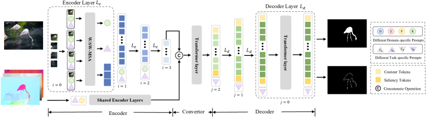
Figure 3: Overall framework of our proposed VSCode model with 2D prompt learning. Based on the VST [62] foundation model, we insert the respective domain-specific prompts and task-specific prompts in the attention windows in the Swin transformer [66] encoder layers to learn domain and task-specific encoder features. The convertor is used for multimodal feature fusion. Within the transformer decoder layers, task-specific prompts are appended to image feature tokens to perform task-specific decoding. We also provide detailed structures of an encoder layer ($i=0$) and a decoder layer ($j=0$).

2.3 Generalist Segmentation Architecture

Recently, several generalist frameworks have emerged for a range of segmentation tasks using a variety of prompts. On one hand, X-Decoder [130] utilized generic non-semantic queries and semantic queries to decode different pixel-level and token-level outputs. UNINEXT [106] introduced three types of prompts, namely category names, language expressions, and reference annotations. On the other hand, Painter [99] and SegGPT [100] leveraged image-mask pairs from the same task as prompts to assist the model in executing individual segmentation tasks. Unlike the approaches mentioned above, which mainly concentrate on task differences, our VSCode dissects unique characteristics based on both domain and task dimensions, leading to a more versatile design.

In the field of SOD and COD, EVP [64] introduced adaptors into the encoder and trained each task individually for various foreground segmentation tasks. Different from them, we consider not only multiple tasks but also multiple modalities. Moreover, our VSCode trains all tasks simultaneously, leading to more sufficient data usage and efficient computational costs, which further distinguish it from EVP.

3 Methodology

In this work, we propose VSCode with the aim of jointly training SOD and COD tasks in an efficient and effective way. We allow VST [62] to incorporate commonalities (Section 3.1), and utilize 2D prompts, which comprise domain-specific (Section 3.2) and task-specific prompts (Section 3.3), to encapsulate peculiarities. To accurately disentangle domain and task peculiarities in 2D prompts and encourage commonality learning in VST, we introduce a prompt discrimination loss (Section 3.5). Figure 3 shows the overall architecture of our proposed VSCode.

3.1 Foundation Model

To achieve a more comprehensive integration of commonalities from SOD and COD tasks, we select VST [62] as our fundamental model. VST was originally proposed for RGB and RGB-D SOD and comprises three primary components, i.e. a transformer encoder, a transformer convertor, and a multi-task transformer decoder. It initially employs the transformer encoder to capture long-range dependencies within the image features $\bm{f}_{i}^{E}\in{\mathbb{R}^{l_{i}\times c_{i}}}$, where $i\in[0,1,2,3]$ indicates the index of blocks in the encoder, $l_{i}$ and $c_{i}$ mean the length of the patch sequence and the channel number of $\bm{f}_{i}^{E}$. Subsequently, the transformer convertor integrates the complement between RGB and depth features via cross-attention for RGB-D SOD or uses self-attention for RGB SOD. In the decoder, which is composed of a sequence of self-attention layers, VST predicts saliency maps and boundary maps simultaneously via a saliency token, a boundary token, and decoder features $\bm{f}_{j}^{D}\in{\mathbb{R}^{l_{j}\times d}}$, where $j$ corresponds the index of blocks in the decoder. Here $j\in[2,1,0]$ for descending order and $d$ =384. Due to the simple and pure-transformer-based architecture, VST can be easily used for other multimodal tasks and COD tasks without the need for model redesign. As a result, it emerges as a superior choice for constructing a generalist model for general multimodal SOD and COD.

In pursuit of improved outcomes and a more suitable structure, we introduce modifications to VST. First, we select Swin transformer [66] as our backbone due to its efficiency and high performance. Second, to maintain a unified structure for both RGB tasks and other multimodal tasks, we utilize the RGB convertor in VST, which comprises standard transformer layers. For multimodal tasks, we simply concatenate the supplementary modality’s features with the RGB features along the channel dimension and employ a multilayer perceptron (MLP) to project them from 2$d$ channels to $d$ channels. For RGB tasks, no alterations are made. Third, we incorporate certain extensions from VST++ [58], specifically including the token-supervised prediction loss.

3.2 Domain-specific Prompt

Within the encoder, lower layers are dedicated to extracting low-level features, encompassing edges, colors, and textures, which exhibit distinct characteristics in various domains [111]. For instance, depth maps are typically rendered in grayscale, while thermal maps present a broader color spectrum. Higher layers, on the other hand, capture semantic information from modality features, which is crucial for all tasks. Consequently, we introduce domain-specific prompts $\bm{p}_{i}^{d}$ at each block $i$ in the encoder and design four kinds of domain-specific prompts for RGB, depth, thermal, and optical flow, respectively, to highlight the disparities among domains, as shown in Figure 3.

Given the image features $\bm{f}_{i}^{E}$ from a specific block in the Swin transformer encoder, we use window-attention [66] and partition the feature $\bm{f}_{i}^{E}$ into window features $\bm{f}_{i\_w}^{E}\in{\mathbb{R}^{l_{i}/M^{2}\times M^{2}\times c_{i}}}$, where $M$ represents the window size and $l_{i}/M^{2}$ is the number of windows. Then, we replicate the prompts $\bm{p}_{i}^{d}\in{\mathbb{R}^{N_{i}\times c_{i}}}$ for each window and obtain $\bm{p}_{i}^{d^{\prime}}\in{\mathbb{R}^{l_{i}/M^{2}\times N_{i}\times c_{i}}}$, where $N_{i}$ represents the number of learnable prompt tokens. Next, we append them to the patch feature tokens in each window and perform self-attention within each window, which can be defined as

$$\begin{bmatrix}\bm{p}_{i+1}^{d^{\prime}}\\ \bm{f}_{i\_w}^{E}\end{bmatrix}\leftarrow\text{MLP}(\text{SW/W-MSA}(\begin{bmatrix}\bm{p}_{i}^{d^{\prime}}\\ \bm{f}_{i\_w}^{E}\end{bmatrix})),$$ (1)

where W-MSA and SW-MSA are multi-head self-attention modules with regular and shifted windowing configurations, respectively. Here we omit the residual connection [27] and layer normalization [1]. Next, we segment $\bm{p}_{i+1}^{d^{\prime}}$ from each window and calculate the average of them to obtain $\bm{p}_{i+1}^{d}$, and then reassemble the output window feature $\bm{f}_{i\_w}^{E}$ to $\bm{f}_{i+1}^{E}$ for the next block.

3.3 Task-specific Prompt

Prior research [47] has traditionally regarded SOD and COD as opposing tasks, emphasizing the disparities between the features extracted by the SOD encoder and the COD encoder as much as possible. However, we believe that SOD and COD share significant commonalities in their features, such as low-level cues, high-level objectness, and spatial structuredness. As a result, we introduce task-specific prompts to learn the peculiarities while retaining the primary stream parameters shared to capture commonalities. We add the task-specific prompts in both VST encoder and decoder, and the overall impact of adding these prompts is illustrated in Figure 4.

\begin{overpic}[width=433.62pt]{Figures/show_example.pdf} \put(7.7,-4.5){\footnotesize Image} \put(27.6,-6.5){\scriptsize\shortstack[c]{Predictions with \\ SOD Prompt}} \put(53.3,-6.5){\scriptsize\shortstack[c]{Predictions with \\ COD Prompt}} \put(82.3,-4.5){\footnotesize COD GT} \end{overpic}

Figure 4: Illustration of the influence of using different task prompts.

Encoder. Although the encoder primarily focuses on domain-specific features with domain prompts, semantic features still play a pivotal role in distinguishing SOD and COD tasks. Semantic features from the encoder typically emphasize the most relevant region for a particular task and allocate more attention accordingly. In the case of the SOD task, the foreground region receives greater attention, whereas for the COD task, the background usually gains large importance since objects are typically concealed within it. Hence, it is essential to incorporate task-specific prompts to encourage learning task-related features in the encoder. Otherwise, we risk initially activating the wrong objects before the decoding process. Following the pattern of domain-specific prompts, we introduce task-specific prompts $\bm{p}_{i}^{te}$ in each encoder block and use them in the same way as how domain-specific prompts are used.

Decoder. Camouflaged objects typically exhibit more intricate and detailed boundaries compared to salient objects. This complexity arises because concealed objects often share structural or textual similarities with their surroundings, resulting in imperceptible boundaries. Therefore, solely introducing task-specific prompts in the encoder may not be adequate, as camouflaged objects require a more refined process within the decoder. We incorporate task-specific prompts in the decoder to allocate distinct attention for reconstructing both the boundary and object regions based on the features extracted by the encoder. In contrast, previous research [47] has not adequately explored the differences between these two tasks in the decoder, as they typically use a single decoder to handle both.

Regarding task-specific prompts in the decoder, we simply append learnable prompts $\bm{p}_{j+1}^{td}$ to the decoder feature tokens $\bm{f}_{j+1}^{D}$ from a specific block $j+1$ in the decoder. Then, we apply the self-attention as follows:

$$\begin{bmatrix}\bm{p}_{j}^{td}\\ \bm{f}_{j}^{D}\\ \end{bmatrix}\leftarrow\text{MLP}(\text{MSA}(\begin{bmatrix}\bm{p}_{j+1}^{td}\\ \bm{f}_{j+1}^{D}\\ \end{bmatrix})),$$ (2)

where MSA denotes the multi-head self-attention. Here we omit the saliency and boundary tokens in the VST decoder for conciseness. Please note that our task-specific prompts differ from saliency and boundary tokens since we do not introduce any supervision for them.

3.4 Prompts Layout and Discussion

To incorporate the aforementioned prompts within the encoder-decoder architecture, inspired by VPT [39], we offer two prompt inserting versions. In the deep version, new prompts are introduced at the start of each transformer block, whereas the shallow version involves proposing prompts at first and updating them across all blocks. To unveil the specific relationship among different domains and tasks at varying network depths, we employ the deep version for both domain and task-specific prompts within the encoder. Based on VST’s design, which introduces a saliency and a boundary token at the beginning of the decoder, we use the shallow version for task-specific prompts in the decoder.

We calculate the correlations of different domain and task prompt pairs at different blocks in Figure 5. It is evident that depth, thermal, and optical flow exhibit relatively strong correlations in low-level features, as all of them usually show obvious low-level contrast between target objects and backgrounds in terms of color or luminance. However, at higher levels, most domains exhibit lower correlations, highlighting the distinctions among them. Additionally, as for task-specific prompts, it is clear that SOD prompts and COD prompts exhibit more shared knowledge in the lower layers. As we progress to higher layers, the correlation decreases, indicating that high-level features gradually learn unrelated information. This observation urges us to implement the deep version of domain-specific prompts and task-specific prompts in the encoder in our final design, as different blocks acquire distinct knowledge. Moreover, the gradually decreased correlation values along with the increase of the network depth encourage us to use a progressively larger number of prompt tokens, as lower correlation means larger peculiarities and hence requires more parameters to learn.

Figure 5: Correlation of prompt pairs at each encoder block.

3.5 Loss Function

The design principle of our model is to use 2D prompts for encompassing peculiarities while integrating commonalities into the foundation model. However, this is not straightforward for freely learned prompts. As shown in Figure 5, they still suggest certain correlations. This indicates that the learned prompts are entangled, risking the model’s capacity to differentiate among various domains and tasks and resulting in suboptimal optimization. Hence, we propose a prompt discrimination loss to minimize the correlation among the prompts of the same type, guaranteeing that each prompt acquires unique domain or task knowledge. Specifically, we aggregate prompts of the same domain/task into a single embedding and then perform discrimination. First, we average the input prompt tokens of each same prompt type at each block and use linear projections to align the channel numbers to $d$. Subsequently, for each type of prompt, we concatenate the averaged prompts of different blocks, and use MLP to obtain the overall domain-specific prompt $p_{l}^{d_{all}}$ and task-specific encoder prompt $p_{k}^{{te}_{all}}$:

$$\begin{split}p_{l}^{d_{all}}=\text{MLP}[\text{LA}(\bm{p}_{0}^{d});\text{LA}(\bm{p}_{1}^{d});\text{LA}({\bm{p}_{2}^{d}});\text{LA}(\bm{p}_{3}^{d})],\\ p_{k}^{{te}_{all}}=\text{MLP}[\text{LA}(\bm{p}_{0}^{te});\text{LA}(\bm{p}_{1}^{te});\text{LA}({\bm{p}_{2}^{te}});\text{LA}(\bm{p}_{3}^{te})],\end{split}$$ (3)

where L and A represent the linear and average operation, respectively, with $l\in\{depth,thermal,flow,rgb\}$, and $k\in\{SOD,COD\}$. Since the task-specific prompts in the decoder are shallow, we simply average them.

Afterward, we calculate the cosine similarity between prompt pairs, resulting in eight types of cosine similarity results $\mathcal{CS}_{m}$. Here $m$ means the combination of domains/tasks, namely $\{RD,RT,RF,DF,DT,TF\}$ for domain-aggregated prompts and $\{SC_{EN},SC_{DE}\}$ for task-aggregated prompts in the encoder and decoder, respectively. Finally, we minimize the correlation within these prompt pairs and define our prompt discrimination loss as

$$\mathcal{L}_{dis}=\sum_{m}\ln(1+|\mathcal{CS}_{m}|),$$ (4)

which is further combined with the segmentation losses and boundary losses [62] to train our model.

4 Experiment

Settings	Params	RGB SOD			RGB-D SOD			RGB-T SOD			VSOD			RGB COD			VCOD
		DUTS[93]			NJUD[41]			VT5000[89]			SegV2[49]			CAMO[45]			CAD[3]
	(M)	$S_{m}\uparrow$	$F_{m}\uparrow$	$E_{m}\uparrow$	$S_{m}\uparrow$	$F_{m}\uparrow$	$E_{m}\uparrow$	$S_{m}\uparrow$	$F_{m}\uparrow$	$E_{m}\uparrow$	$S_{m}\uparrow$	$F_{m}\uparrow$	$E_{m}\uparrow$	$S_{m}\uparrow$	$F_{m}\uparrow$	$E_{m}\uparrow$	$S_{m}\uparrow$	$F_{m}\uparrow$	$E_{m}\uparrow$
ST	323.46	.900	.885	.940	.927	.928	.958	.900	.863	.938	.896	.870	.952	.793	.751	.871	.686	.522	.787
GT	54.06	.898	.884	.941	.924	.922	.954	.903	.886	.942	.930	.911	.972	-	-	-	-	-	-
GT+$p^{d}$	54.06	.902	.890	.945	.931	.932	.962	.909	.877	.947	.931	.917	.975	-	-	-	-	-	-
GT+$p^{d}$+$p^{t}$	54.09	.904	.892	.945	.931	.931	.961	.906	.892	.946	.925	.910	.970	.804	.776	.876	.759	.639	.808
GT+$\bm{p^{d}}$+$\bm{p^{t}}$+$\bm{\mathcal{L}_{dis}}$	54.09	.909	.899	.948	.935	.938	.965	.912	.882	.950	.943	.930	.984	.811	.782	.884	.736	.614	.797
w/o $p^{te}$	54.07	.908	.896	.947	.932	.932	.960	.909	.878	.947	.933	.907	.966	.800	.770	.872	.743	.611	.798
w/o $p^{td}$	54.08	.902	.889	.943	.929	.929	.959	.904	.872	.941	.940	.919	.975	.799	.770	.875	.740	.599	.814

Table 1: Ablation studies of our VSCode on the Swin-T [66] backbone with $224\times 224$ image size. We conduct evaluations on one representative dataset for each task. “ST” indicates special training, “GT” means general training, $p^{d}$ represents domain-specific prompts, and $p^{t}$ is task-specific prompts, which consists of $p^{te}$ in the encoder and $p^{td}$ in the decoder. $\mathcal{L}_{dis}$ is our prompt discrimination loss. The best results under each setting are labeled in bold.

Settings	Params	RGB SOD			RGB-D SOD			RGB-T SOD			VSOD			RGB COD			VCOD
		DUTS[93]			NJUD[41]			VT5000[89]			SegV2[49]			CAMO[45]			CAD[3]
	(M)	$S_{m}\uparrow$	$F_{m}\uparrow$	$E_{m}\uparrow$	$S_{m}\uparrow$	$F_{m}\uparrow$	$E_{m}\uparrow$	$S_{m}\uparrow$	$F_{m}\uparrow$	$E_{m}\uparrow$	$S_{m}\uparrow$	$F_{m}\uparrow$	$E_{m}\uparrow$	$S_{m}\uparrow$	$F_{m}\uparrow$	$E_{m}\uparrow$	$S_{m}\uparrow$	$F_{m}\uparrow$	$E_{m}\uparrow$
shallow or deep version for domain-specific prompts
shallow	54.83	.900	.887	.943	.926	.926	.955	.905	.873	.944	.931	.917	.972	-	-	-	-	-	-
deep	54.06	.902	.890	.945	.931	.932	.962	.909	.877	.947	.931	.917	.975	-	-	-	-	-	-
shallow or deep version for task-specific prompts in the encoder
shallow	54.45	.902	.888	.943	.928	.928	.958	.902	.870	.940	.927	.905	.964	.793	.763	.866	.747	.616	.798
deep	54.08	.903	.890	.944	.934	.934	.962	.905	.874	.943	.924	.903	.960	.804	.772	.881	.759	.651	.831
shallow or deep version for task-specific prompts in the decoder
deep	54.10	.903	.891	.945	.930	.932	.960	.905	.888	.943	.922	.903	.966	.802	.774	.881	.738	.605	.801
shallow	54.09	.904	.892	.945	.930	.931	.961	.906	.892	.946	.925	.910	.970	.804	.776	.876	.759	.639	.808
number of domain-specific prompts at four blocks
1,1,1,1	54.06	.902	.890	.945	.931	.932	.962	.909	.877	.947	.931	.917	.975	-	-	-	-	-	-
5,5,5,5	54.08	.903	.890	.945	.931	.935	.961	.902	.869	.940	.918	.887	.954	-	-	-	-	-	-
number of task-specific prompts in the encoder at four blocks
5,5,5,5	54.07	.903	.893	.947	.928	.930	.959	.903	.870	.940	.931	.918	.975	.795	.766	.866	.739	.600	.799
1,1,5,10	54.08	.903	.890	.944	.934	.934	.962	.905	.874	.943	.924	.903	.960	.804	.772	.881	.759	.651	.831
number of task-specific prompts in the decoder
5	54.08	.904	.890	.946	.929	.931	.957	.904	.890	.943	.931	.911	.969	.807	.782	.881	.746	.626	.805
10	54.09	.904	.892	.945	.930	.931	.961	.906	.892	.946	.925	.910	.970	.804	.776	.876	.759	.639	.808
15	54.09	.903	.889	.944	.929	.933	.956	.904	.890	.942	.932	.913	.974	.798	.771	.875	.743	.621	.791

Table 2: Ablation studies of different designs of prompt layout.

4.1 Datasets and Evaluation Metrics

For RGB SOD, we evaluate our proposed model using six commonly used benchmark datasets, i.e. DUTS [93], ECSSD [108], HKU-IS [53], PASCAL-S [55], DUT-O [110], and SOD [70]. For RGB-D SOD, we use six large benchmark datasets, including STERE [72], NJUD [41], NLPR [78], DUTLF-Depth [80], SIP [18], and ReDWeb-S [61]. In terms of RGB-T SOD, we consider three public datasets: VT821 [91], VT1000 [90], and VT5000 [89]. For VSOD, we employ six widely used benchmark datasets: DAVIS [79], FBMS [73], ViSal [97], SegV2 [49], DAVSOD-Easy, and DAVSOD-Normal [19]. Regarding RGB COD, three extensive benchmark datasets are considered, including COD10K [16], CAMO [45], and NC4K [69]. For VCOD, we utilize two widely accepted benchmark datasets: CAD [3] and MoCA-Mask [11]. To ensure a consistent evaluation across all SOD and COD tasks, we employ three commonly used evaluation metrics to assess model performance: structure-measure $S_{m}$ [14], maximum enhanced-alignment measure $E_{m}$ [15], and maximum F-measure $F_{m}$.

4.2 Implementation Details

Building on prior research [62, 89, 59, 26, 11], we employ the following datasets to train our model concurrently: the training set of DUTS for RGB SOD, the training sets of NJUD, NLPR, and DUTLF-Depth for RGB-D SOD, the training set of VT5000 for RGB-T SOD, the training sets of DAVIS and DAVSOD for VSOD, the training sets of COD10K and CAMO for RGB COD, and the training set of MoCA-Mask for VCOD. To ensure a fair comparison with previous works [129, 46, 88, 64, 26], we resize each image to $384\times 384$ pixels and then randomly crop them to $352\times 352$ image regions for training. Our training process employs the Adam optimizer [43] with an initial learning rate of 0.0001, which is reduced by a factor of 10 at half and three-quarters of the total training steps. We conduct a total of 150,000 training steps using a 3090 GPU. We mix the above six tasks in each training iteration with two samples for each task, leading to a total batch size of 12.

Summary	Params	DUTS[93]			ECSSD[108]			HKU-IS[53]			PASCAL-S[55]			DUT-O[110]			SOD[70]
	(M)	$S_{m}\uparrow$	$F_{m}\uparrow$	$E_{m}\uparrow$	$S_{m}\uparrow$	$F_{m}\uparrow$	$E_{m}\uparrow$	$S_{m}\uparrow$	$F_{m}\uparrow$	$E_{m}\uparrow$	$S_{m}\uparrow$	$F_{m}\uparrow$	$E_{m}\uparrow$	$S_{m}\uparrow$	$F_{m}\uparrow$	$E_{m}\uparrow$	$S_{m}\uparrow$	$F_{m}\uparrow$	$E_{m}\uparrow$
VST[62]	44.48	.896	.877	.939	.932	.944	.964	.928	.937	.968	.873	.850	.900	.850	.800	.888	.854	.866	.902
ICON-R[129]	33.09	.890	.876	.931	.928	.943	.960	.920	.931	.960	.862	.844	.888	.845	.799	.884	.848	.861	.899
VST-T++ [58]	53.60	.901	.887	.943	.937	.949	.968	.930	.939	.968	.878	.855	.901	.853	.804	.892	.853	.866	.899
MENet[101]	27.83	.905	.895	.943	.927	.938	.956	.927	.939	.965	.871	.848	.892	.850	.792	.879	.841	.847	.884
VSCode-T	54.09	.917	.910	.954	.945	.957	.971	.935	.946	.970	.878	.852	.900	.869	.830	.910	.863	.879	.908
EVP[64]	64.52	.917	.910	.956	.936	.949	.965	.935	.945	.971	.880	.859	.902	.864	.822	.902	.854	.873	.901
VSCode-S	74.72	.926	.922	.960	.949	.959	.974	.940	.951	.974	.887	.864	.904	.877	.840	.912	.870	.882	.910

Table 3: Quantitative comparison of our VSCode with other 5 SOTA RGB SOD methods on six benchmark datasets. “-R”, “-T” and “-S” mean the ResNet50 [27], Swin-T, and Swin-S[66] backbones, respectively. ‘-’ indicates the code is not available. The best performance under all settings is bolded, and the best results under each setting are labeled in bold.

Summary	Params	NJUD [41]			NLPR[78]			DUTLF-Depth[80]			ReDWeb-S[61]			STERE[72]			SIP[18]
	(M)	$S_{m}\uparrow$	$F_{m}\uparrow$	$E_{m}\uparrow$	$S_{m}\uparrow$	$F_{m}\uparrow$	$E_{m}\uparrow$	$S_{m}\uparrow$	$F_{m}\uparrow$	$E_{m}\uparrow$	$S_{m}\uparrow$	$F_{m}\uparrow$	$E_{m}\uparrow$	$S_{m}\uparrow$	$F_{m}\uparrow$	$E_{m}\uparrow$	$S_{m}\uparrow$	$F_{m}\uparrow$	$E_{m}\uparrow$
CMINet[113]	188.12	.929	.934	.957	.932	.922	.963	.912	.913	.938	.725	.726	.800	.918	.916	.951	.899	.910	.939
VST[62]	53.83	.922	.920	.951	.932	.920	.962	.943	.948	.969	.759	.763	.826	.913	.907	.951	.904	.915	.944
VST-T++ [58]	100.51	.928	.929	.958	.933	.921	.964	.944	.948	.969	.756	.757	.819	.916	.911	.950	.903	.914	.944
SPSN[46]	-	-	-	-	.923	.912	.960	-	-	-	-	-	-	.907	.902	.945	.892	.900	.936
CAVER[77]	55.79	.920	.924	.953	.929	.921	.964	.931	.939	.962	.730	.724	.802	.914	.911	.951	.893	.906	.934
VSCode-T	54.09	.941	.945	.967	.938	.930	.966	.952	.959	.974	.766	.771	.831	.928	.926	.957	.917	.936	.955
VSCode-S	74.72	.944	.949	.970	.941	.932	.968	.960	.967	.980	.777	.776	.829	.931	.928	.958	.924	.942	.958

Table 4: Quantitative comparison of our VSCode with other 5 SOTA RGB-D SOD methods on six benchmark datasets.

Summary	Params	VT821[91]			VT1000[90]			VT5000[89]
	(M)	$S_{m}$	$F_{m}$	$E_{m}$	$S_{m}$	$F_{m}$	$E_{m}$	$S_{m}$	$F_{m}$	$E_{m}$
MIDD[88]	52.43	.871	.847	.916	.916	.904	.956	.868	.834	.919
TNet[12]	87.41	.899	.885	.936	.929	.921	.965	.895	.864	.936
CGMDR[7]	-	.894	.872	.932	.931	.927	.966	.896	.877	.939
VST-T++ [58]	100.51	.894	.861	.923	.941	.931	.972	.895	.854	.933
CAVER[77]	55.79	.891	.874	.933	.936	.927	.970	.892	.857	.935
VSCode-T	54.09	.921	.906	.951	.949	.944	.981	.918	.892	.954
VSCode-S	74.72	.926	.910	.954	.952	.947	.981	.925	.900	.959

Table 5: Quantitative comparison of our VSCode with other 5 SOTA RGB-T SOD methods on three benchmark datasets.

Summary	Params	DAVIS [79]			FBMS[73]			ViSal[97]			SegV2[49]			DAVSOD-Easy[19]			DAVSOD-Normal[19]
	(M)	$S_{m}\uparrow$	$F_{m}\uparrow$	$E_{m}\uparrow$	$S_{m}\uparrow$	$F_{m}\uparrow$	$E_{m}\uparrow$	$S_{m}\uparrow$	$F_{m}\uparrow$	$E_{m}\uparrow$	$S_{m}\uparrow$	$F_{m}\uparrow$	$E_{m}\uparrow$	$S_{m}\uparrow$	$F_{m}\uparrow$	$E_{m}\uparrow$	$S_{m}\uparrow$	$F_{m}\uparrow$	$E_{m}\uparrow$
DCFNet[116]	71.66	.914	.899	.970	.883	.853	.910	.952	.953	.990	.903	.870	.953	.729	.612	.781	.708	.601	.791
FSNet[35]	102.30	.922	.909	.972	.875	.867	.918	-	-	-	.849	.773	.920	.760	.637	.796	.732	.623	.789
CoSTFormer[59]	-	.923	.906	.978	-	-	-	-	-	-	.874	.813	.943	.779	.667	.819	.730	.614	.777
UFO[86]	55.92	.918	.906	.978	.858	.868	.911	.926	.917	.969	.888	.850	.951	.747	.626	.799	.711	.605	.773
VSCode-T	54.09	.930	.913	.970	.891	.880	.923	.952	.954	.989	.943	.937	.984	.792	.696	.831	.738	.631	.797
VSCode-S	74.72	.936	.922	.973	.905	.902	.939	.955	.957	.991	.946	.937	.984	.800	.710	.835	.758	.666	.815

Table 6: Quantitative comparison of our VSCode with other 4 SOTA VSOD methods on six benchmark datasets.

Summary	Params	COD10K[16]			NC4K[69]			CAMO[45]
	(M)	$S_{m}$	$F_{m}$	$E_{m}$	$S_{m}$	$F_{m}$	$E_{m}$	$S_{m}$	$F_{m}$	$E_{m}$
MGL[112]	63.60	.814	.738	.890	-	-	-	.776	.741	.842
UJSC[47]	121.63	.817	.750	.902	.856	.835	.920	.803	.775	.867
SegMar[40]	56.21	.833	.755	.907	.841	.827	.907	.816	.803	.884
FEDER[26]	44.13	.822	.768	.905	.847	.833	.915	.802	.789	.873
VSCode-T	54.09	.847	.795	.925	.874	.853	.930	.838	.821	.909
EVP[64]	64.52	.845	.794	.926	.874	.855	.933	.849	.833	.918
VSCode-S	74.72	.869	.827	.942	.891	.878	.944	.873	.861	.938

Table 7: Quantitative comparison of our VSCode with other 5 SOTA RGB COD methods on three benchmark datasets.

Summary	Params	CAD [3]			MoCA-Mask[11]
	(M)	$S_{m}\uparrow$	$F_{m}\uparrow$	$E_{m}\uparrow$	$S_{m}\uparrow$	$F_{m}\uparrow$	$E_{m}\uparrow$
PNS-Net[34]	26.87	.671	.473	.787	.514	.068	.599
RCRNet[107]	53.79	.664	.405	.786	.559	.170	.593
MG[109]	-	.608	.378	.673	.500	.138	.514
SLT-Net[11]	164.68	.715	.542	.823	.624	.327	.768
VSCode-T	54.09	.757	.659	.808	.650	.339	.787
VSCode-S	74.72	.790	.680	.853	.665	.386	.796

Table 8: Quantitative comparison of our VSCode with other 4 SOTA VCOD methods on two benchmark datasets.

4.3 Ablation Study

Architecture Design.

To demonstrate the efficacy of various components in our VSCode model, we report the quantitative results in Table 1. We start by performing special training (ST) on each task individually and then conduct general training (GT) on all SOD tasks. Please note that here we do not consider COD tasks since no task prompt is used. We observe improved performance on RGB-T SOD and VSOD, demonstrating the significant benefit of shared knowledge in different tasks, especially for those with limited training data diversity. However, the results of RGB SOD and RGB-D SOD do not show a significant increase. Our hypothesis is that amalgamating the training of multimodal images within a shared model might prevent further optimization on those well-learned tasks. Based on this, we introduce domain-specific prompts $p^{d}$, resulting in substantial improvements across all datasets, which demonstrates the efficacy of domain-specific prompts in consolidating peculiarities within their respective domains. Subsequently, we introduce task-specific prompts $p^{t}$ in the encoder-decoder architecture, enabling the capability to handle COD tasks. This brings slightly improved performance on some SOD tasks, however, significantly improves the performance on all COD tasks compared with the ST baseline, which probably owes to the well-learned commonalities from different tasks. Moreover, the incorporation of the prompt discrimination loss $\mathcal{L}_{dis}$ leads to improved performance on most tasks, reaffirming its effectiveness in disentangling peculiarities.

To further evaluate the effectiveness of the task-specific prompts in the encoder and decoder, we remove them individually, resulting in performance decrease. This indicates that using task prompts in both encoder and decoder is necessary. We also observe our 2D prompts only bring around 0.03M parameters, which makes our model much more parameter-efficient than the traditional special training scheme.

Prompt Location.

Following VPT [39], we design other forms of prompt layout based on Section 3.4. Table 2 reveals that employing the shallow version of task-specific prompts in the decoder, the deep version of domain-specific prompts and task-specific prompts in the encoder yields the best results. One plausible rationale is that each block aggregates distinct-level features within the encoder, thus it is better to propose unique prompts for each block. In our decoder, we follow VST and used skip connection to fuse decoder features with encoder features, which have already utilized deep task prompts for distinction. Hence, using more task prompts in the decoder may not be essential, and the shallow version seems to be a more fitting choice.

Prompt Length.

We perform experiments with varying lengths for three kinds of prompts. As shown in Table 2, for domain-specific prompts, using one prompt token at each block achieves better performance than using more tokens. This suggests that it’s possible to effectively capture domain distinctions using only a small number of prompts, which matches the observed relatively large correlation within domain prompts in Figure 5. Regarding task-specific prompts within the encoder, a prompt layout of 1,1,5,10 tokens at four blocks is found to be optimal on COD tasks, highlighting the importance of high-level semantic features over low-level features in distinguishing between SOD and COD tasks. This observation matches Figure 5 as well in which the correlations of SC in deep blocks are smaller than those in shallow blocks. Regarding the number of task-specific prompts in the decoder, performance starts to decline when it exceeds 10. This emphasizes that blindly increasing the number of prompts doesn’t guarantee improved performance.

4.4 Comparison with State-of-the-Art Methods

Due to space limitation, we only report the performance comparison of our methods against other most highly-performed state-of-the-art methods, including 4 specialist RGB SOD models [62, 129, 101, 58], 5 specialist RGB-D SOD models [113, 62, 46, 77, 58], 5 specialist RGB-T SOD models [88, 12, 7, 77, 58], 3 specialist VSOD models [116, 35, 59], 4 specialist RGB COD models [112, 47, 40, 26], and 4 specialist VCOD models [34, 107, 109, 11]. Two generalist models [64, 86] are also reported. To ensure a relatively fair comparison with EVP [64], which utilizes SegFormer-B4 [105] as their backbone (64.1M parameters), we switch our backbone to Swin-S [66] as it has a similar number of parameters (50M). As shown in Table 3, Table 4, Table 5, Table 6, Table 7, and Table 8, our VSCode significantly outperforms all specialist methods and two generalist models across all six tasks, underscoring the effectiveness of our specially designed 2D prompts and prompt discrimination loss. The supplementary material displays visual comparison results among the top-performing models.

4.5 Analysis of Generalization Ability

Previous generalist research [64, 86] primarily concentrated on assessing the effectiveness of models in training tasks, neglecting their capacity for generalizing to novel tasks. Therefore, we employ the RGB-D COD task, which is not used in training, to further investigate the zero-shot generalization capabilities of our model. Specifically, we utilize our well-trained model and combine depth and COD prompts to tackle the RGB-D COD task. As shown in Table 9, our VSCode model significantly outperforms the state-of-the-art specialist model PopNet [104], although ours works in a pure zero-shot way. This demonstrates the superior zero-shot generalization ability of our proposed method. We also present the results of our model using only RGB information, which yields considerably lower performance compared to zero-shot RGB-D results. This validates that our zero-shot performance is not reliant on the utilization of seen RGB COD information but on the effectiveness of consolidating domain- and task-specific knowledge, which allows for the straightforward combination of various domain- and task-specific prompts for unseen tasks.

Summary		COD10K[16]			NC4K[69]			CAMO[45]
Method	Task	$S_{m}$	$F_{m}$	$E_{m}$	$S_{m}$	$F_{m}$	$E_{m}$	$S_{m}$	$F_{m}$	$E_{m}$
PopNet[104]	RGB-D	.851	.802	.919	.861	.843	.919	.808	.792	.874
VSCode-T	ZS RGB-D	.882	.849	.945	.902	.894	.950	.885	.885	.945
VSCode-T	RGB	.847	.795	.925	.874	.853	.930	.838	.821	.909

Table 9: Comparison with the SOTA RGB-D COD method on three benchmark datasets. “ZS” indicates zero-shot.

5 Conclusion

In this paper, we present VSCode, a novel generalist and parameter-efficient model that tackles general multimodal SOD and COD tasks. Concretely, we use a foundation model to assimilate commonalities and 2D prompts to learn domain and task peculiarities. Furthermore, a prompt discrimination loss is introduced to help effectively disentangle specific knowledge and learn better shared knowledge. Our experiments demonstrate the effectiveness of VSCode on six training tasks and one unseen task.

Appendix A1 Additional Implementation Details

For VSOD and VCOD tasks, we follow the common practice of utilizing Flownet2.0 [32] as the optical flow extractor due to its consistently strong performance. It is worth noting that our results for the VSOD task may differ significantly from previous studies. This discrepancy is due to our adoption of a PyTorch-based toolbox for evaluating all tasks, whereas previous methods relied on a MATLAB-based toolbox which has different implementation details.

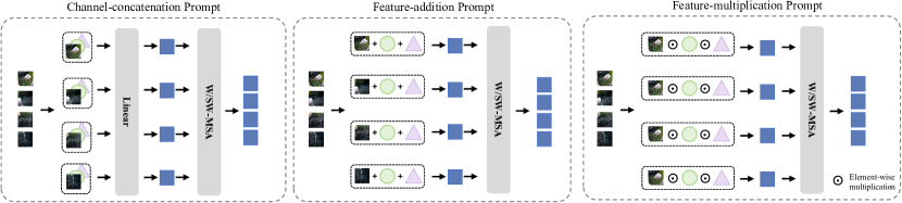
Figure A1: Proposed channel-concatenation prompt, feature-addition prompt, and feature-multiplication prompt.

Appendix A2 Prompt Design Variants

We further investigate different types of prompts and conduct an analysis of their parameter counts. For computational efficiency, we limit our design to simple learnable prompts based on attention mechanism in the encoder, as shown in Figure A1.

A2.1 Channel-concatenation Prompt

To maintain consistency in the fusion technique across RGB and other modalities, we suggest using learnable channel-concatenation prompt $\bm{p}_{i}^{c}\in{\mathbb{R}^{1\times c_{i}}}$. We concatenate the $\bm{p}_{i}^{c}$ with the image feature $\bm{f}_{i}^{E}$ along the channel dimension and utilize a linear projection to project them back to the original channel number. The entire process is expressed as follows:

$$\bm{f}_{i}^{E}=\text{Linear}([\bm{f}_{i}^{E};\bm{p}_{i}^{c}]),$$ (A1)

where $[;]$ indicates the concatenation operation and Linear means linear projection. Since the parameters of the linear operation can be expressed as $2c_{i}*c_{i}+c_{i}=2c_{i}^{2}+c_{i}$, and the parameters for the channel-concatenation prompt are $1*c_{i}$. Therefore, the total number of parameters for the channel-concatenation prompt becomes $\sum_{i}2c_{i}^{2}+2c_{i}$.

A2.2 Feature-addition Prompt

In ViPT [64], prompts are introduced by incorporating carefully designed layers and added to the inputs. To emphasize simple and learnable prompt, we refer to these addition computational forms and introduce feature-addition prompt $\bm{p}_{i}^{a}\in{\mathbb{R}^{1\times c_{i}}}$ for the image features $\bm{f}_{i}^{E}$:

$$\bm{f}_{i}^{E}=\bm{f}_{i}^{E}+\bm{p}_{i}^{a}.$$ (A2)

The feature-addition prompt can capture domain- or task-specific details for pixels. The total parameters for the feature-addition prompt amount to $c_{i}$.

A2.3 Feature-multiplication Prompt

In segmentation tasks, masks are commonly employed to consolidate object information and extract distinct features [10]. Expanding on this concept, we utilize feature-multiplication prompt $\bm{p}_{i}^{m}\in{\mathbb{R}^{1\times c_{i}}}$ as the mask query and apply them to the image features. This operation is computed as follows:

$$\bm{f}_{i}^{E}=\bm{f}_{i}^{E}\odot\bm{p}_{i}^{m}.$$ (A3)

The feature-multiplication prompt selectively extracts domain-specific or task-specific information from image features. In the case of the feature-multiplication prompt, the total number of parameters is also $c_{i}$.

We conduct experiments on domain-specific prompts using the aforementioned prompt forms, as shown in Table A1. Our token-concatenation prompt uses fewer parameters while delivering superior results, demonstrating the efficiency of our design. This also underscores that the concatenation design maximizes feature variations for different tasks and domains compared to addition and multiplication.

Settings	Params	RGB SOD			RGBD SOD			RGBT SOD			VSOD
		DUTS[93]			NJUD[41]			VT5000[89]			SegV2[49]
	(M)	$S_{m}\uparrow$	$F_{m}\uparrow$	$E_{m}\uparrow$	$S_{m}\uparrow$	$F_{m}\uparrow$	$E_{m}\uparrow$	$S_{m}\uparrow$	$F_{m}\uparrow$	$E_{m}\uparrow$	$S_{m}\uparrow$	$F_{m}\uparrow$	$E_{m}\uparrow$
channel-concatenation prompt	57.22	.798	.744	.852	.881	.870	.917	.846	.799	.898	.822	.744	.911
feature-addition prompt	54.09	.892	.875	.935	.924	.922	.956	.890	.854	.930	.899	.860	.945
feature-multiplication prompt	54.09	.732	.657	.793	.870	.858	.910	.792	.720	.847	.811	.706	.915
token-concatenation prompt	54.09	.902	.890	.945	.931	.932	.962	.909	.877	.947	.931	.917	.975

Table A1: Ablation studies of different prompt design variants on the Swin-T backbone [66] with $224\times 224$ image size. We conduct evaluations on one representative dataset for each task.

Settings	Params	RGB SOD			RGBD SOD			RGBT SOD			VSOD			RGB COD			VCOD
		DUTS[93]			NJUD[41]			VT5000[89]			SegV2[49]			CAMO[45]			CAD[3]
	(M)	$S_{m}\uparrow$	$F_{m}\uparrow$	$E_{m}\uparrow$	$S_{m}\uparrow$	$F_{m}\uparrow$	$E_{m}\uparrow$	$S_{m}\uparrow$	$F_{m}\uparrow$	$E_{m}\uparrow$	$S_{m}\uparrow$	$F_{m}\uparrow$	$E_{m}\uparrow$	$S_{m}\uparrow$	$F_{m}\uparrow$	$E_{m}\uparrow$	$S_{m}\uparrow$	$F_{m}\uparrow$	$E_{m}\uparrow$
margin = 0.2	54.09	.908	.897	.948	.933	.934	.961	.911	.880	.949	.937	.927	.979	.811	.786	.889	.734	.616	.817
margin = 0.1	54.09	.907	.897	.948	.931	.933	.960	.911	.881	.949	.935	.920	.976	.810	.781	.884	.725	.588	.800
margin = 0	54.09	.909	.899	.948	.935	.938	.965	.912	.882	.950	.943	.930	.984	.811	.782	.884	.736	.614	.797

Table A2: Ablation studies of the prompt discrimination loss settings with different margins using $224\times 224$ image size.

Appendix A3 Further Ablation Study

A3.1 Effectiveness of the Prompt Discrimination Loss

In fact, our prompt discrimination loss can be viewed as a specific instance of the hinge loss with a margin set to 0. To further evaluate its effectiveness, we present a more general expression

$$\mathcal{L}_{dis}=\sum_{m}\ln(1+\max\{|\mathcal{CS}_{m}|,margin\}).$$ (A4)

When the margin is greater than 0, it indicates that the loss doesn’t impose any constraints on prompts when the correlation is below the margin. In other words, it signifies a higher degree of shared knowledge among different domains and tasks.

Since the correlation between different domains and tasks ranges from 0 to 0.26 when prompt discrimination loss is not applied, as shown in Figure 5 in the main text, we set margins of 0.1 and 0.2 to illustrate the effectiveness of our design. The results can be found in Table A2. Overall, the results obtained with a margin of 0 outperform other designs, providing evidence of the effectiveness of fully disentangling different domain and task knowledge in our joint learning approach.

However, setting the margin as 0 shows a decrease in COD tasks. This can be attributed to the significantly fewer training data available for COD tasks (7915 training images) compared to SOD tasks (30450 training images), which means COD tasks need more shared knowledge learned from the SOD data. Hence, attempting to completely separate SOD and COD knowledge might further compromise performance in COD tasks. In our future work, we will explore methods to balance the relationship between tasks and ensure comprehensive training for all tasks.

Appendix A4 Deeper Analysis of Generalization Capacity

To further investigate our model’s zero-shot generalization, we reserved separate tasks for zero-shot evaluation and retrained our model on other tasks. Recognizing the risk of overfitting when training with limited data, we evaluated the zero-shot capability using the RGB COD task and the RGB-D SOD task for single-modality task and SOD task, respectively (10553 training images for RGB SOD v.s 4040 for RGB COD, 4040 training images for RGB-D COD v.s 2985 for RGB-D SOD).

Summary	Task	NJUD [41]			NLPR[78]			DUTLF-Depth[80]			ReDWeb-S[61]			STERE[72]			SIP[18]
		$S_{m}$	$F_{m}$	$E_{m}$	$S_{m}$	$F_{m}$	$E_{m}$	$S_{m}$	$F_{m}$	$E_{m}$	$S_{m}$	$F_{m}$	$E_{m}$	$S_{m}$	$F_{m}$	$E_{m}$	$S_{m}$	$F_{m}$	$E_{m}$
CMINet[113]	RGB-D	.929	.934	.957	.932	.922	.963	.912	.913	.938	.725	.726	.800	.918	.916	.951	.899	.910	.939
VST[62]	RGB-D	.922	.920	.951	.932	.920	.962	.943	.948	.969	.759	.763	.826	.913	.907	.951	.904	.915	.944
VST-T++ [58]	RGB-D	.928	.929	.958	.933	.921	.964	.944	.948	.969	.756	.757	.819	.916	.911	.950	.903	.914	.944
SPSN[46]	RGB-D	-	-	-	.923	.912	.960	-	-	-	-	-	-	.907	.902	.945	.892	.900	.936
CAVER[77]	RGB-D	.920	.924	.953	.929	.921	.964	.931	.939	.962	.730	.724	.802	.914	.911	.951	.893	.906	.934
VSCode-T	ZS RGB-D	.910	.912	.941	.912	.887	.940	.931	.936	.956	.746	.733	.809	.908	.904	.937	.925	.939	.963
VSCode-T	RGB-D	.941	.945	.967	.938	.930	.966	.952	.959	.974	.766	.771	.831	.928	.926	.957	.917	.936	.955

Table A3: Quantitative comparison of our proposed VSCode with other 5 out-performing RGB-D SOD methods on six benchmark datasets.“ZS” indicates zero-shot.

Summary	Task	COD10K[16]			NC4K[69]			CAMO[45]
		$S_{m}$	$F_{m}$	$E_{m}$	$S_{m}$	$F_{m}$	$E_{m}$	$S_{m}\uparrow$	$F_{m}$	$E_{m}$
UJSC[47]	RGB	.817	.750	.902	.856	.835	.920	.803	.775	.867
SegMar[40]	RGB	.833	.755	.907	.841	.827	.907	.816	.803	.884
FEDER[26]	RGB	.822	.768	.905	.847	.833	.915	.802	.789	.873
VSCode-T	ZS RGB	.836	.778	.916	.870	.850	.926	.830	.805	.904
VSCode-T	RGB	.847	.795	.925	.874	.853	.930	.838	.821	.909

Table A4: Quantitative comparison of our proposed VSCode with other SOTA RGB COD methods on three benchmark datasets.“ZS” indicates zero-shot.

As depicted in Table A4, even without training with the RGB COD task, our VSCode model still outperforms state-of-the-art task-specific RGB COD models, although it works in a zero-shot way. This indicates that our model relies not only on the effectiveness of domain-specific prompts in segregating domain knowledge, but also on the accuracy of our task-specific prompts in integrating task-related knowledge. However, for the RGB-D SOD task, the performance of our zero-shot VSCode lags behind that of state-of-the-art task-specific training methods, as shown in Table A3. We hypothesize that this is because the depth maps of RGB-D COD datasets are generated using an off-the-shelf depth estimation model [82], which is different from most RGB-D SOD datasets that use real depth maps captured by Microsoft Kinect (e.g. NLPR [78]), light field cameras (e.g. DUTLF-Depth [80]), and smartphones (e.g. SIP [18]). The estimated depth maps of RGB-D COD might lack certain high-quality geometric cues for real scenarios, leading to incomplete depth knowledge for depth prompts. Despite our zero-shot performance in the RGB-D SOD task not outperforming state-of-the-art methods, the comparable performance still highlights the generalization ability of our VSCode when encountering unseen tasks.

Appendix A5 More Comparison Results

To conserve space, we focus on presenting state-of-the-art methods from 2021 in the main text. In this section, we provide a more comprehensive comparison of state-of-the-art methods dating back to 2018, as shown in Table A5, Table A6, Table A7, Table A8, Table A9, and Table A10. We also introduce an additional evaluation metric, the mean absolute error ($M$), to assess model performance. Furthermore, we include various versions of our VSCode with different backbones for comparison with other models. For instance, VSCode-B utilizes the Swin-B backbone [66] and demonstrates exceptional performance compared to the VSCode-T and VSCode-S versions. Here, we compare our VSCode-B with FSPNet [30] in the RGB COD task, which employs a backbone with similar parameters to Swin-B [66], i.e. DeiT-B [87].

It’s worth noting that we omit comparisons with some state-of-the-art methods for RGB COD. For example, DCOFD [124] employs a significantly larger image size of 416, which exceeds our approach’s specifications. ZoomNet [75] and MFFN [123] use multi-scale input images. All these settings lead to an unfair comparison with our method.

Appendix A6 Visual Comparison with State-of-the-art Methods

In this section, we provide visual comparison results alongside state-of-the-art methods for four SOD tasks (RGB SOD, RGB-D SOD, RGB-T SOD, and VSOD) and three COD tasks (RGB COD, VCOD, and RGB-D COD). The results, as depicted in Figure A2, Figure A3, Figure A4, Figure A5, Figure A6, Figure A7, and Figure A8, showcase the exceptional capabilities of our VSCode model across a variety of challenging scenarios. These scenarios include handling significantly small and large objects, multiple objects, occluded objects, and situations with uncertain boundaries, where existing methods often encounter difficulties.

Summary	Backbone	Params	DUTS[93]				ECSSD[108]				HKU-IS[53]				PASCAL-S[55]				DUT-O[110]				SOD[70]
		(M)	$S_{m}$	$F_{m}$	$E_{m}$	$M$	$S_{m}$	$F_{m}$	$E_{m}$	$M$	$S_{m}$	$F_{m}$	$E_{m}$	$M$	$S_{m}$	$F_{m}$	$E_{m}$	$M$	$S_{m}$	$F_{m}$	$E_{m}$	$M$	$S_{m}$	$F_{m}$	$E_{m}$	$M$
PiCANet[57]	ResNet50	47.22	.863	.840	.915	.040	.916	.929	.953	.035	.905	.913	.951	.031	.846	.824	.882	.071	.826	.767	.865	.054	.813	.824	.871	.073
AFNet[21]	VGG16	35.95	.867	.838	.910	.045	.914	.924	.947	.042	.905	.910	.949	.036	.849	.824	.877	.076	.826	.759	.861	.057	.811	.819	.867	.085
TSPOANet[65]	VGG16	-	.860	.828	.907	.049	.907	.919	.942	.047	.902	.909	.950	.039	.841	.817	.871	.082	.818	.750	.858	.062	.802	.809	.852	.094
EGNet-R[121]	ResNet50	111.64	.887	.866	.926	.039	.925	.936	.955	.037	.918	.923	.956	.031	.852	.825	.874	.080	.841	.778	.878	.053	.824	.831	.875	.080
ITSD-R[125]	ResNet50	26.47	.885	.867	.929	.041	.925	.939	.959	.035	.917	.926	.960	.031	.861	.839	.889	.771	.840	.792	.880	.061	.835	.849	.889	.075
MINet-R[76]	ResNet50	162.38	.884	.864	.926	.037	.925	.938	.957	.034	.919	.926	.960	.029	.856	.831	.883	.071	.883	.769	.869	.056	.830	.835	.878	.074
LDF-R[102]	ResNet50	25.15	.892	.877	.930	.034	.925	.938	.954	.034	.920	.929	.958	.028	.861	.839	.888	.067	.839	.782	.870	.052	.831	.841	.878	.071
CSF-R2[24]	Res2Net50	36.53	.890	.869	.929	.037	.931	.942	.960	.033	-	-	-	-	.863	.839	.885	.073	.838	.775	.869	.055	.826	.832	.883	.079
GateNet-R[122]	ResNet50	128.63	.891	.874	.932	.038	.924	.935	.955	.038	.921	.926	.959	.031	.863	.836	.886	.071	.840	.782	.878	.055	.827	.835	.877	.079
VST[62]	T2T-ViTt-14	44.48	.896	.877	.939	.037	.932	.944	.964	.034	.928	.937	.968	.030	.873	.850	.900	.067	.850	.800	.888	.058	.854	.866	.902	.065
ICON-R[129]	ResNet50	33.09	.890	.876	.931	.037	.928	.943	.960	.032	.920	.931	.960	.029	.862	.844	.888	.071	.845	.799	.884	.057	.848	.861	.899	.067
VST-T++ [58]	Swin-T	53.60	.901	.887	.943	.033	.937	.949	.968	.029	.930	.939	.968	.026	.878	.855	.901	.063	.853	.804	.892	.053	.853	.866	.899	.065
MENet[101]	ResNet50	27.83	.905	.895	.943	.028	.927	.938	.956	.031	.927	.939	.965	.023	.871	.848	.892	.062	.850	.792	.879	.045	.841	.847	.884	.065
VSCode-T	Swin-T	54.09	.917	.910	.954	.027	.945	.957	.971	.024	.935	.946	.970	.024	.878	.852	.900	.062	.869	.830	.910	.045	.863	.879	.908	.056
EVP[64]	SegFormer-B4	64.52	.917	.910	.956	.027	.936	.949	.965	.029	.935	.945	.971	.024	.880	.859	.902	.061	.864	.822	.902	.047	.854	.873	.901	.065
VSCode-S	Swin-S	74.72	.926	.922	.960	.024	.949	.959	.974	.022	.940	.951	.974	.021	.887	.864	.904	.058	.877	.840	.912	.043	.870	.882	.910	.054
VSCode-B	Swin-B	117.41	.932	.930	.965	.022	.949	.961	.974	.022	.941	.951	.974	.021	.890	.866	.906	.056	.880	.846	.913	.043	.871	.882	.910	.056

Table A5: Quantitative comparison of our proposed VSCode with other 14 SOTA RGB SOD methods on six benchmark datasets. “-R”,“-R2”, “-T”, “-S”, and “-B” mean the ResNet50 [27], Res2Net [23], SwinT-1k, SwinS-22k, and SwinB-22k[66] backbones, respectively. ‘-’ indicates the code is not available. The best performance under all settings is bolded, and the best results under each setting are labeled in bold.

Summary	Backbone	Params	NJUD [41]				NLPR[78]				DUTLF-Depth[80]				ReDWeb-S[61]				STERE[72]				SIP[18]
		(M)	$S_{m}$	$F_{m}$	$E_{m}$	$M$	$S_{m}$	$F_{m}$	$E_{m}$	$M$	$S_{m}$	$F_{m}$	$E_{m}$	$M$	$S_{m}$	$F_{m}$	$E_{m}$	$M$	$S_{m}$	$F_{m}$	$E_{m}$	$M$	$S_{m}$	$F_{m}$	$E_{m}$	$M$
ATST[115]	VGG19	32.17	.885	.893	.930	.047	.909	.898	.951	.027	.916	.928	.953	.033	.679	.673	.758	.155	.896	.901	.942	.038	.849	.861	.901	.063
CMW[51]	VGG16	85.56	.870	.871	.927	.061	.917	.903	.951	.029	.797	.779	.864	.098	.634	.607	.714	.195	.852	.837	.907	.067	.705	.677	.804	.141
Cas-Gnn[68]	VGG16	-	.911	.916	.948	.036	.919	.906	.955	.025	.920	.926	.953	.030	-	-	-	-	.899	.901	.944	.039	-	-	-	-
HDFNet[74]	ResNet50	44.15	.908	.911	.944	.039	.923	.917	.963	.023	.908	.915	.945	.041	.728	.717	.804	.129	.900	.900	.943	.042	.886	.894	.930	.048
CoNet[37]	ResNet50	43.66	.896	.893	.937	.046	.912	.893	.948	.027	.923	.932	.959	.029	.696	.693	.782	.147	.905	.901	.947	.037	.860	.873	.917	.058
BBS-Net[20]	ResNet50	49.77	.921	.919	.949	.035	.931	.918	.961	.023	.882	.870	.912	.058	.693	.680	.763	.150	.908	.903	.942	.041	.879	.884	.922	.055
JL-DCF[22]	VGG16	143.52	.877	.892	.941	.066	.931	.918	.965	.022	.894	.891	.927	.048	.581	.546	.708	.213	.900	.895	.942	.044	0.885	.894	.931	.049
SPNet[126]	Res2Net50	67.88	.925	.928	.957	.029	.927	.919	.962	.021	.895	.899	.933	.045	.710	.715	.798	.129	.907	.906	.949	.037	.894	.904	.933	.043
CMINet[113]	ResNet50	188.12	.929	.934	.957	.029	.932	.922	.963	.021	.912	.913	0938	.038	.725	.726	.800	.121	.918	.916	.951	.032	.899	.910	.939	.040
DCF[36]	ResNet50	53.92	.904	.905	.943	.039	.922	.910	.957	.024	.925	.930	.956	.030	.709	.715	.790	.135	.906	.904	.948	.037	.874	.886	.922	.052
VST[62]	T2T-ViTt-14	53.83	.922	.920	.951	.035	.932	.920	.962	.024	.943	.948	.969	.024	.759	.763	.826	.113	.913	.907	.951	.038	.904	.915	.944	.040
VST-T++ [58]	Swin-T	100.51	.928	.929	.958	.031	.933	.921	.964	.022	.944	.948	.969	.024	.756	.757	.819	.114	.916	.911	.950	.037	.903	.914	.944	.039
SPSN[46]	VGG16	-	-	-	-	-	.923	.912	.960	.023	-	-	-	-	-	-	-	-	.907	.902	.945	.036	.892	.900	.936	.043
CAVER[77]	ResNet50	55.79	.920	.924	.953	.032	.929	.921	.964	.022	.931	.939	.962	.028	.730	.724	.802	.121	.914	.911	.951	.034	.893	.906	.934	.043
VSCode-T	Swin-T	54.09	.941	.945	.967	.025	.938	.930	.966	.020	.952	.959	.974	.019	.766	.771	.831	.105	.928	.926	.957	.030	.917	.936	.955	.032
VSCode-S	Swin-S	74.72	.944	.949	.970	.022	.941	.932	.968	.018	.960	.967	.980	.015	.777	.776	.829	.100	.931	.928	.958	.028	.924	.942	.958	.029
VSCode-B	Swin-B	117.41	.944	.950	.969	.023	.944	.939	.971	.017	.959	.967	.978	.017	.772	.771	.828	.101	.933	.931	.960	.028	.913	.936	.950	.034

Table A6: Quantitative comparison of our proposed VSCode with other 14 SOTA RGB-D SOD methods on six benchmark datasets.

Summary	Backbone	Params	VT821[91]				VT1000[90]				VT5000[89]
		(M)	$S_{m}$	$F_{m}$	$E_{m}$	$M$	$S_{m}$	$F_{m}$	$E_{m}$	$M$	$S_{m}$	$F_{m}$	$E_{m}$	$M$
FCMF[118]	VGG16	-	.760	.667	.810	.081	.873	.851	.921	.037	0.814	.758	.866	.055
ADF[89]	VGG16	-	.808	.749	.841	.077	.909	.908	.950	.034	.863	.837	.911	.048
ECFFNet[127]	ResNet34	-	.877	.835	.911	.034	.924	.919	.959	0.021	.876	.850	.922	.037
CGFNet[92]	VGG16	69.92	.881	.866	.920	.038	.923	.923	.959	.023	.883	.852	.926	.039
CSRNet[31]	ESPNetv2	1.01	.885	.855	.920	.037	.919	.901	.952	.027	.868	.821	.912	.045
MGAI[85]	Res2Net50	87.09	.891	.870	.933	.030	.929	.921	.965	.024	.884	.846	.930	.037
MIDD[88]	VGG16	52.43	.871	.847	.916	.044	.916	.904	.956	.030	.868	.834	.919	.045
TNet[12]	ResNet50	87.41	.899	.885	.936	.030	.929	.921	.965	.024	.895	.864	.936	.036
CGMDRNet[7]	Res2Net50	-	.894	.872	.932	.035	.931	.927	.966	.020	.896	.877	.939	.032
VST-T++ [58]	Swin-T	100.51	.894	.861	.923	.034	.941	.931	.972	.020	.895	.854	.933	.037
CAVER[77]	ResNet50	55.79	.891	.874	.933	.033	.936	.927	.970	.021	.892	.857	.935	.035
VSCode-T	Swin-T	54.09	.921	.906	.951	.021	.949	.944	.981	.017	.918	.892	.954	.028
VSCode-S	Swin-S	74.72	.926	.910	.954	.021	.952	.947	.981	.016	.925	.900	.959	.026
VSCode-B	Swin-B	117.41	.928	.915	.956	.021	.953	.949	.984	.016	.930	.907	.962	.025

Table A7: Quantitative comparison of our proposed VSCode with other 11 SOTA RGB-T SOD methods on three benchmark datasets.

Summary	Backbone	Params	DAVIS [79]				FBMS[73]				ViSal[97]				SegV2[49]				DAVSOD-Easy[19]				DAVSOD-Normal[19]
		(M)	$S_{m}$	$F_{m}$	$E_{m}$	$M$	$S_{m}$	$F_{m}$	$E_{m}$	$M$	$S_{m}$	$F_{m}$	$E_{m}$	$M$	$S_{m}$	$F_{m}$	$E_{m}$	$M$	$S_{m}$	$F_{m}$	$E_{m}$	$M$	$S_{m}$	$F_{m}$	$E_{m}$	$M$
PDB[84]	ResNet50	-	.880	.851	.949	.030	.850	.821	.882	.072	.926	.922	.970	.024	.871	.820	.867	.024	-	-	-	-	-	-	-	-
FGRN[52]	VGGNet	-	.839	.786	.918	.043	.822	.783	.871	.084	.867	.852	.954	.041	.737	.660	.904	.037	-	-	-	-	-	-	-	-
RCRNet[107]	ResNet50	53.79	.884	.845	.947	.028	.873	.850	.902	.055	.933	.925	.971	.020	.829	.747	.901	.038	.726	.601	.773	.078	0.692	.550	.760	.102
SSAV[19]	ResNet50	-	.891	.857	.945	.029	.880	.856	.922	.043	.944	.940	.983	.018	.934	.797	.922	.024	-	-	-	-	-	-	-	-
PCSA[25]	MobileNetV3	2.63	.901	.878	.961	.023	.874	.847	.914	.043	.946	.941	.984	.016	.887	.850	.940	.019	.725	.590	.759	.077	-	-	-	-
DCFNet[116]	ResNet101	71.66	.914	.899	.970	.016	.883	.853	.910	.041	.952	.953	.990	.010	.903	.870	.953	.013	.729	.612	.781	.065	.708	.601	.791	.077
FSNet[35]	ResNet50	102.3	.922	.909	.972	.019	.875	.867	.918	.048	-	-	-	-	.849	.773	.920	.023	.760	.637	.796	.063	.732	.623	.789	.088
CoSTFormer[59]	ResNet50	-	.923	.906	.978	.014	-	-	-	-	-	-	-	-	.874	.813	.943	.018	.779	.667	.819	.060	.730	.614	.777	.082
UFO[86]	VGG16	55.92	.918	.906	.978	.015	.858	.868	.911	.051	.926	.917	.969	.020	.888	.850	.951	.014	.747	.626	.799	.063	.711	.605	.773	.088
VSCode-T	Swin-T	54.09	.930	.913	.970	.014	.891	.880	.923	.037	.952	.954	.989	.010	.943	.937	.984	.008	.792	.696	.831	.053	.738	.631	.797	.078
VSCode-S	Swin-S	74.72	.936	.922	.973	.013	.905	.902	.939	.029	.955	.957	.991	.009	.946	.937	.984	.008	.800	.710	.835	.052	.758	.666	.815	.071
VSCode-B	Swin-B	117.41	.936	.923	.974	.014	.900	.901	.940	.031	.957	.948	.991	.009	.947	.937	.984	.008	.812	.728	.847	.047	.769	.690	.845	.069

Table A8: Quantitative comparison of our proposed VSCode with other 9 SOTA VSOD methods on six benchmark datasets.

Summary	Backbone	Params	COD10K[16]				NC4K[69]				CAMO[45]
		(M)	$S_{m}$	$F_{m}$	$E_{m}$	$M$	$S_{m}$	$F_{m}$	$E_{m}$	$M$	$S_{m}$	$F_{m}$	$E_{m}$	$M$
SINet[16]	ResNet50	48.95	.771	.676	.868	.051	.808	.775	.883	.058	.752	.706	.831	.100
CRLS[69]	ResNet50	-	.805	.732	.892	.037	.840	.815	.907	.048	.787	.753	.854	.080
MGL[112]	ResNet50	63.60	.814	.738	.890	.035	-	-	-	-	.776	.741	.842	.089
UJSC[47]	ResNet50	121.63	.817	.750	.902	.033	.856	.835	.920	.040	.803	.775	.867	.071
SegMar[40]	ResNet50	56.21	.833	.755	.907	.034	.841	.827	.907	.046	.816	.803	.884	.071
FEDER[26]	ResNet50	44.13	.822	.768	.905	.032	.847	.833	.915	.044	.802	.789	.873	.071
VSCode-T	Swin-T	54.09	.847	.795	.925	.028	.874	.853	.930	.038	.838	.821	.909	.060
EVP[64]	SegFormer-B4	64.52	.845	.794	.926	.029	.874	.855	.933	.039	.849	.833	.918	.058
VSCode-S	Swin-S	74.72	.869	.827	.942	.024	.891	.878	.944	.032	.873	.861	.938	.047
FSPNet	DeiT-B	274.24	.851	.794	.931	.026	.879	.859	.937	.035	.856	.846	.928	.050
VSCode-B	Swin-B	117.41	.876	.838	.947	.022	.902	.892	.952	.029	.882	.875	.940	.044

Table A9: Quantitative comparison of our proposed VSCode with other 8 SOTA RGB COD methods on three benchmark datasets.

Summary	Backbone	Params	CAD [3]				MoCA-Mask[11]
		(M)	$S_{m}$	$F_{m}$	$E_{m}$	$M$	$S_{m}$	$F_{m}$	$E_{m}$	$M$
PNS-Net[34]	Res2Net50	26.87	.671	.473	.787	.054	.514	.068	.599	.030
RCRNet[107]	ResNet50	53.79	.664	.405	.786	.051	.559	.170	.593	.025
MG[109]	VGG	-	.608	.378	.673	.069	.500	.138	.514	.078
SLT-Net[11]	PVT	164.68	.715	.542	.823	.036	.624	.327	.768	.019
VSCode-T	Swin-T	54.09	.757	.659	.808	.034	.650	.339	.787	.013
VSCode-S	Swin-S	74.72	.790	.680	.853	.026	.665	.386	.796	.012
VSCode-B	Swin-B	117.41	.791	.678	.852	.027	.678	.430	.832	.011

Table A10: Quantitative comparison of our proposed VSCode with other 4 SOTA VCOD methods on two benchmark datasets.

\begin{overpic}[width=433.62pt]{Figures/RGB.pdf} \put(3.0,-1.6){\footnotesize Image} \put(13.7,-1.6){\footnotesize GT} \put(21.6,-1.6){\footnotesize VSCode-T} \put(31.3,-1.6){\footnotesize VSCode-S} \put(43.0,-3.2){\footnotesize\shortstack[c]{EVP \\ \cite[cite]{[\@@bibref{Number}{liu2023explicit}{}{}]}}} \put(53.1,-3.2){\footnotesize\shortstack[c]{MENet\\ \cite[cite]{[\@@bibref{Number}{wang2023pixels}{}{}]}}} \put(62.7,-3.2){\footnotesize\shortstack[c]{VST++ \\ \cite[cite]{[\@@bibref{Number}{liu2023vst++}{}{}]}}} \put(72.3,-3.2){\footnotesize\shortstack[c]{ICON-R \\ \cite[cite]{[\@@bibref{Number}{zhuge2021salient}{}{}]}}} \put(82.8,-3.2){\footnotesize\shortstack[c]{VST\\ \cite[cite]{[\@@bibref{Number}{Liu_2021_ICCV}{}{}]}}} \put(91.5,-3.2){\footnotesize\shortstack[c]{GateNet-R\\ \cite[cite]{[\@@bibref{Number}{GateNet}{}{}]}}} \end{overpic}

Figure A2: Qualitative comparison of our model against state-of-the-art RGB SOD methods. (GT: ground truth.)

\begin{overpic}[width=433.62pt]{Figures/RGBD.pdf} \put(3.0,-1.6){\footnotesize Image} \put(13.2,-1.6){\footnotesize Depth} \put(23.8,-1.6){\footnotesize GT} \put(31.3,-1.6){\footnotesize VSCode-T} \put(43.0,-3.2){\footnotesize\shortstack[c]{CAVER \\ \cite[cite]{[\@@bibref{Number}{pang2023caver}{}{}]}}} \put(53.1,-3.2){\footnotesize\shortstack[c]{SPSN\\ \cite[cite]{[\@@bibref{Number}{lee2022spsn}{}{}]}}} \put(62.7,-3.2){\footnotesize\shortstack[c]{VST++ \\ \cite[cite]{[\@@bibref{Number}{liu2023vst++}{}{}]}}} \put(72.8,-3.2){\footnotesize\shortstack[c]{VST \\ \cite[cite]{[\@@bibref{Number}{Liu_2021_ICCV}{}{}]}}} \put(82.8,-3.2){\footnotesize\shortstack[c]{DCF\\ \cite[cite]{[\@@bibref{Number}{Ji_2021_DCF}{}{}]}}} \put(91.5,-3.2){\footnotesize\shortstack[c]{CMINEet\\ \cite[cite]{[\@@bibref{Number}{cascaded_rgbd_sod}{}{}]}}} \end{overpic}

Figure A3: Qualitative comparison of our model against state-of-the-art RGB-D SOD methods. (GT: ground truth.)

\begin{overpic}[width=433.62pt]{Figures/RGBT.pdf} \put(3.0,-1.6){\footnotesize Image} \put(11.5,-1.6){\footnotesize Thermal} \put(23.7,-1.6){\footnotesize GT} \put(31.5,-1.6){\footnotesize VSCode-T} \put(42.5,-3.2){\footnotesize\shortstack[c]{CAVER \\ \cite[cite]{[\@@bibref{Number}{pang2023caver}{}{}]}}} \put(53.1,-3.2){\footnotesize\shortstack[c]{TNet\\ \cite[cite]{[\@@bibref{Number}{cong2022does}{}{}]}}} \put(62.7,-3.2){\footnotesize\shortstack[c]{MIDD \\ \cite[cite]{[\@@bibref{Number}{tu2021multi}{}{}]}}} \put(72.5,-3.2){\footnotesize\shortstack[c]{MGAI \\ \cite[cite]{[\@@bibref{Number}{song2022multiple}{}{}]}}} \put(82.5,-3.2){\footnotesize\shortstack[c]{CSRNet \\ \cite[cite]{[\@@bibref{Number}{huo2021efficient}{}{}]}}} \put(92.5,-3.2){\footnotesize\shortstack[c]{CGFNet \\ \cite[cite]{[\@@bibref{Number}{wang2021cgfnet}{}{}]}}} \end{overpic}

Figure A4: Qualitative comparison of our model against state-of-the-art RGB-T SOD methods. (GT: ground truth.)

\begin{overpic}[width=433.62pt]{Figures/RGBV.pdf} \put(3.0,-1.6){\footnotesize Image} \put(12.5,-1.6){\footnotesize Flow} \put(21.0,-1.6){\footnotesize GT} \put(28.0,-1.6){\footnotesize VSCode-T} \put(38.8,-3.2){\footnotesize\shortstack[c]{UFO \\ \cite[cite]{[\@@bibref{Number}{su2023unified}{}{}]}}} \put(45.5,-3.2){\footnotesize\shortstack[c]{CoSTFormer \\ \cite[cite]{[\@@bibref{Number}{liu2023learning}{}{}]}}} \put(57.1,-3.2){\footnotesize\shortstack[c]{FSNet \\ \cite[cite]{[\@@bibref{Number}{ji2021full}{}{}]}}} \put(65.7,-3.2){\footnotesize\shortstack[c]{DCFNet \\ \cite[cite]{[\@@bibref{Number}{zhang2021dynamic}{}{}]}}} \put(75.0,-3.2){\footnotesize\shortstack[c]{SSAV \\ \cite[cite]{[\@@bibref{Number}{fan2019shifting}{}{}]}}} \put(84.3,-3.2){\footnotesize\shortstack[c]{PDB \\ \cite[cite]{[\@@bibref{Number}{song2018pyramid}{}{}]}}} \put(92.5,-3.2){\footnotesize\shortstack[c]{MBN \\ \cite[cite]{[\@@bibref{Number}{li2018unsupervised}{}{}]}}} \end{overpic}

Figure A5: Qualitative comparison of our model against state-of-the-art VSOD methods.(GT: ground truth.)

\begin{overpic}[width=433.62pt]{Figures/COD_RGB.pdf} \put(3.0,-1.6){\footnotesize Image} \put(13.5,-1.6){\footnotesize GT} \put(21.5,-1.6){\footnotesize VSCode-T} \put(32.5,-3.2){\footnotesize\shortstack[c]{FEDER \\ \cite[cite]{[\@@bibref{Number}{he2023camouflaged}{}{}]}}} \put(42.5,-3.2){\footnotesize\shortstack[c]{SegMar \\ \cite[cite]{[\@@bibref{Number}{jia2022segment}{}{}]}}} \put(52.1,-3.2){\footnotesize\shortstack[c]{ZoomNet \\ \cite[cite]{[\@@bibref{Number}{pang2022zoom}{}{}]}}} \put(62.7,-3.2){\footnotesize\shortstack[c]{UJSC \\ \cite[cite]{[\@@bibref{Number}{li2021uncertainty}{}{}]}}} \put(72.9,-3.2){\footnotesize\shortstack[c]{MGL \\ \cite[cite]{[\@@bibref{Number}{zhai2021mutual}{}{}]}}} \put(83.0,-3.2){\footnotesize\shortstack[c]{CRLS \\ \cite[cite]{[\@@bibref{Number}{lv2021simultaneously}{}{}]}}} \put(92.9,-3.2){\footnotesize\shortstack[c]{SINet \\ \cite[cite]{[\@@bibref{Number}{fan2020camouflaged}{}{}]}}} \end{overpic}

Figure A6: Qualitative comparison of our model against state-of-the-art RGB COD methods.(GT: ground truth.)

\begin{overpic}[width=433.62pt]{Figures/VCOD.pdf} \put(4.0,-1.6){\footnotesize Image} \put(17.0,-1.6){\footnotesize Flow} \put(30.3,-1.6){\footnotesize GT} \put(40.0,-1.6){\footnotesize VSCode-T} \put(53.5,-3.2){\footnotesize\shortstack[c]{PNS-Net \\ \cite[cite]{[\@@bibref{Number}{ji2021progressively}{}{}]}}} \put(66.5,-3.2){\footnotesize\shortstack[c]{RCRNet \\ \cite[cite]{[\@@bibref{Number}{yan2019semi}{}{}]}}} \put(79.3,-3.2){\footnotesize\shortstack[c]{MG \\ \cite[cite]{[\@@bibref{Number}{yang2021self}{}{}]}}} \put(90.7,-3.2){\footnotesize\shortstack[c]{SLT-Net \\ \cite[cite]{[\@@bibref{Number}{cheng2022implicit}{}{}]}}} \end{overpic}

Figure A7: Qualitative comparison of our model against state-of-the-art VCOD methods.(GT: ground truth.)

\begin{overpic}[width=433.62pt]{Figures/COD_RGBD.pdf} \put(9.0,-1.6){\footnotesize Image} \put(28.5,-1.6){\footnotesize Depth} \put(48.6,-1.6){\footnotesize GT} \put(66.6,-1.6){\footnotesize VSCode-T} \put(86.5,-3.2){\footnotesize\shortstack[c]{PopNet \\ \cite[cite]{[\@@bibref{Number}{wu2023source}{}{}]}}} \end{overpic}

Figure A8: Qualitative comparison of our model against state-of-the-art RGB-D COD methods.(GT: ground truth.)

References

- [1] Jimmy Lei Ba, Jamie Ryan Kiros, and Geoffrey E Hinton. Layer normalization. arXiv preprint arXiv:1607.06450, 2016.
- [2] Hyojin Bahng, Ali Jahanian, Swami Sankaranarayanan, and Phillip Isola. Exploring visual prompts for adapting large-scale models. arXiv preprint arXiv:2203.17274, 2022.
- [3] Pia Bideau and Erik Learned-Miller. It’s moving! a probabilistic model for causal motion segmentation in moving camera videos. In ECCV, pages 433–449. Springer, 2016.
- [4] Pia Bideau, Rakesh R Menon, and Erik Learned-Miller. Moa-net: self-supervised motion segmentation. In ECCV, pages 0–0, 2018.
- [5] Ali Borji, Ming-Ming Cheng, Qibin Hou, Huaizu Jiang, and Jia Li. Salient object detection: A survey. CVMJ, 5:117–150, 2019.
- [6] Tom Brown, Benjamin Mann, Nick Ryder, Melanie Subbiah, Jared D Kaplan, Prafulla Dhariwal, Arvind Neelakantan, Pranav Shyam, Girish Sastry, Amanda Askell, et al. Language models are few-shot learners. NeurIPS, 33:1877–1901, 2020.
- [7] Gang Chen, Feng Shao, Xiongli Chai, Hangwei Chen, Qiuping Jiang, Xiangchao Meng, and Yo-Sung Ho. Cgmdrnet: Cross-guided modality difference reduction network for rgb-t salient object detection. TCSVT, 32(9):6308–6323, 2022.
- [8] Shuhan Chen and Yun Fu. Progressively guided alternate refinement network for rgb-d salient object detection. In ECCV, pages 520–538, 2020.
- [9] Zuyao Chen, Runmin Cong, Qianqian Xu, and Qingming Huang. Dpanet: Depth potentiality-aware gated attention network for rgb-d salient object detection. IEEE TIP, 2020.
- [10] Bowen Cheng, Ishan Misra, Alexander G Schwing, Alexander Kirillov, and Rohit Girdhar. Masked-attention mask transformer for universal image segmentation. In CVPR, pages 1290–1299, 2022.
- [11] Xuelian Cheng, Huan Xiong, Deng-Ping Fan, Yiran Zhong, Mehrtash Harandi, Tom Drummond, and Zongyuan Ge. Implicit motion handling for video camouflaged object detection. In CVPR, pages 13864–13873, 2022.
- [12] Runmin Cong, Kepu Zhang, Chen Zhang, Feng Zheng, Yao Zhao, Qingming Huang, and Sam Kwong. Does thermal really always matter for rgb-t salient object detection? TMM, 2022.
- [13] Zijun Deng, Xiaowei Hu, Lei Zhu, Xuemiao Xu, Jing Qin, Guoqiang Han, and Pheng-Ann Heng. R3net: Recurrent residual refinement network for saliency detection. In IJCAI, pages 684–690, 2018.
- [14] Deng-Ping Fan, Ming-Ming Cheng, Yun Liu, Tao Li, and Ali Borji. Structure-measure: A new way to evaluate foreground maps. In ICCV, pages 4548–4557, 2017.
- [15] Deng-Ping Fan, Cheng Gong, Yang Cao, Bo Ren, Ming-Ming Cheng, and Ali Borji. Enhanced-alignment Measure for Binary Foreground Map Evaluation. In IJCAI, pages 698–704, 2018.
- [16] Deng-Ping Fan, Ge-Peng Ji, Guolei Sun, Ming-Ming Cheng, Jianbing Shen, and Ling Shao. Camouflaged object detection. In CVPR, pages 2777–2787, 2020.
- [17] Deng-Ping Fan, Ge-Peng Ji, Peng Xu, Ming-Ming Cheng, Christos Sakaridis, and Luc Van Gool. Advances in deep concealed scene understanding. Visual Intelligence, 1(1):16, 2023.
- [18] Deng-Ping Fan, Zheng Lin, Zhao Zhang, Menglong Zhu, and Ming-Ming Cheng. Rethinking rgb-d salient object detection: Models, data sets, and large-scale benchmarks. IEEE TNNLS, 32(5):2075–2089, 2020.
- [19] Deng-Ping Fan, Wenguan Wang, Ming-Ming Cheng, and Jianbing Shen. Shifting more attention to video salient object detection. In CVPR, pages 8554–8564, 2019.
- [20] Deng-Ping Fan, Yingjie Zhai, Ali Borji, Jufeng Yang, and Ling Shao. Bbs-net: Rgb-d salient object detection with a bifurcated backbone strategy network. In ECCV, pages 275–292, 2020.
- [21] Mengyang Feng, Huchuan Lu, and Errui Ding. Attentive feedback network for boundary-aware salient object detection. In CVPR, pages 1623–1632, 2019.
- [22] Keren Fu, Deng-Ping Fan, Ge-Peng Ji, and Qijun Zhao. Jl-dcf: Joint learning and densely-cooperative fusion framework for rgb-d salient object detection. In CVPR, pages 3052–3062, 2020.
- [23] Shang-Hua Gao, Ming-Ming Cheng, Kai Zhao, Xin-Yu Zhang, Ming-Hsuan Yang, and Philip Torr. Res2net: A new multi-scale backbone architecture. IEEE TPAMI, 43(2):652–662, 2019.
- [24] Shang-Hua Gao, Yong-Qiang Tan, Ming-Ming Cheng, Chengze Lu, Yunpeng Chen, and Shuicheng Yan. Highly efficient salient object detection with 100k parameters. In ECCV, pages 702–721, 2020.
- [25] Yuchao Gu, Lijuan Wang, Ziqin Wang, Yun Liu, Ming-Ming Cheng, and Shao-Ping Lu. Pyramid constrained self-attention network for fast video salient object detection. In AAAI, volume 34, pages 10869–10876, 2020.
- [26] Chunming He, Kai Li, Yachao Zhang, Longxiang Tang, Yulun Zhang, Zhenhua Guo, and Xiu Li. Camouflaged object detection with feature decomposition and edge reconstruction. In CVPR, pages 22046–22055, 2023.
- [27] Kaiming He, Xiangyu Zhang, Shaoqing Ren, and Jian Sun. Deep residual learning for image recognition. In CVPR, pages 770–778, 2016.
- [28] Q Hou, MM Cheng, X Hu, A Borji, Z Tu, and PHS Torr. Deeply supervised salient object detection with short connections. IEEE TPAMI, 41(4):815–828, 2018.
- [29] Qidong Huang, Xiaoyi Dong, Dongdong Chen, Weiming Zhang, Feifei Wang, Gang Hua, and Nenghai Yu. Diversity-aware meta visual prompting. In CVPR, pages 10878–10887, 2023.
- [30] Zhou Huang, Hang Dai, Tian-Zhu Xiang, Shuo Wang, Huai-Xin Chen, Jie Qin, and Huan Xiong. Feature shrinkage pyramid for camouflaged object detection with transformers. In CVPR, pages 5557–5566, 2023.
- [31] Fushuo Huo, Xuegui Zhu, Lei Zhang, Qifeng Liu, and Yu Shu. Efficient context-guided stacked refinement network for rgb-t salient object detection. IEEE TCSVT, 32(5):3111–3124, 2021.
- [32] Eddy Ilg, Nikolaus Mayer, Tonmoy Saikia, Margret Keuper, Alexey Dosovitskiy, and Thomas Brox. Flownet 2.0: Evolution of optical flow estimation with deep networks. In ICCV, pages 2462–2470, 2017.
- [33] Jitesh Jain, Jiachen Li, Mang Tik Chiu, Ali Hassani, Nikita Orlov, and Humphrey Shi. Oneformer: One transformer to rule universal image segmentation. In CVPR, pages 2989–2998, 2023.
- [34] Ge-Peng Ji, Yu-Cheng Chou, Deng-Ping Fan, Geng Chen, Huazhu Fu, Debesh Jha, and Ling Shao. Progressively normalized self-attention network for video polyp segmentation. In MICCAI, pages 142–152. Springer, 2021.
- [35] Ge-Peng Ji, Keren Fu, Zhe Wu, Deng-Ping Fan, Jianbing Shen, and Ling Shao. Full-duplex strategy for video object segmentation. In ICCV, pages 4922–4933, 2021.
- [36] Wei Ji, Jingjing Li, Shuang Yu, Miao Zhang, Yongri Piao, Shunyu Yao, Qi Bi, Kai Ma, Yefeng Zheng, Huchuan Lu, and Li Cheng. Calibrated rgb-d salient object detection. In CVPR, pages 9471–9481, June 2021.
- [37] Wei Ji, Jingjing Li, Miao Zhang, Yongri Piao, and Huchuan Lu. Accurate rgb-d salient object detection via collaborative learning. In ECCV, pages 52–69, 2020.
- [38] Yuzhu Ji, Haijun Zhang, Zequn Jie, Lin Ma, and QM Jonathan Wu. Casnet: A cross-attention siamese network for video salient object detection. TNNLS, 32(6):2676–2690, 2020.
- [39] Menglin Jia, Luming Tang, Bor-Chun Chen, Claire Cardie, Serge Belongie, Bharath Hariharan, and Ser-Nam Lim. Visual prompt tuning. In ECCV, pages 709–727. Springer, 2022.
- [40] Qi Jia, Shuilian Yao, Yu Liu, Xin Fan, Risheng Liu, and Zhongxuan Luo. Segment, magnify and reiterate: Detecting camouflaged objects the hard way. In CVPR, pages 4713–4722, 2022.
- [41] Ran Ju, Ling Ge, Wenjing Geng, Tongwei Ren, and Gangshan Wu. Depth saliency based on anisotropic center-surround difference. In ICIP, pages 1115–1119, 2014.
- [42] Alex Kendall, Yarin Gal, and Roberto Cipolla. Multi-task learning using uncertainty to weigh losses for scene geometry and semantics. In CVPR, pages 7482–7491, 2018.
- [43] Diederik P Kingma and Jimmy Ba. Adam: A method for stochastic optimization. arXiv preprint arXiv:1412.6980, 2014.
- [44] Hala Lamdouar, Charig Yang, Weidi Xie, and Andrew Zisserman. Betrayed by motion: Camouflaged object discovery via motion segmentation. In ACCV, 2020.
- [45] Trung-Nghia Le, Tam V Nguyen, Zhongliang Nie, Minh-Triet Tran, and Akihiro Sugimoto. Anabranch network for camouflaged object segmentation. CVIU, 184:45–56, 2019.
- [46] Minhyeok Lee, Chaewon Park, Suhwan Cho, and Sangyoun Lee. Spsn: Superpixel prototype sampling network for rgb-d salient object detection. In ECCV, pages 630–647. Springer, 2022.
- [47] Aixuan Li, Jing Zhang, Yunqiu Lv, Bowen Liu, Tong Zhang, and Yuchao Dai. Uncertainty-aware joint salient object and camouflaged object detection. In CVPR, pages 10071–10081, 2021.
- [48] Aixuan Li, Jing Zhang, Yunqiu Lv, Tong Zhang, Yiran Zhong, Mingyi He, and Yuchao Dai. Joint salient object detection and camouflaged object detection via uncertainty-aware learning. arXiv preprint arXiv:2307.04651, 2023.
- [49] Fuxin Li, Taeyoung Kim, Ahmad Humayun, David Tsai, and James M Rehg. Video segmentation by tracking many figure-ground segments. In ICCV, pages 2192–2199, 2013.
- [50] Gongyang Li, Zhi Liu, and Haibin Ling. Icnet: Information conversion network for rgb-d based salient object detection. IEEE TIP, 29:4873–4884, 2020.
- [51] Gongyang Li, Zhi Liu, Linwei Ye, Yang Wang, and Haibin Ling. Cross-modal weighting network for rgb-d salient object detection. In ECCV, pages 665–681, 2020.
- [52] Guanbin Li, Yuan Xie, Tianhao Wei, Keze Wang, and Liang Lin. Flow guided recurrent neural encoder for video salient object detection. In CVPR, pages 3243–3252, 2018.
- [53] Guanbin Li and Yizhou Yu. Visual saliency based on multiscale deep features. In CVPR, pages 5455–5463, 2015.
- [54] Siyang Li, Bryan Seybold, Alexey Vorobyov, Xuejing Lei, and C-C Jay Kuo. Unsupervised video object segmentation with motion-based bilateral networks. In ECCV, pages 207–223, 2018.
- [55] Yin Li, Xiaodi Hou, Christof Koch, James M Rehg, and Alan L Yuille. The secrets of salient object segmentation. In CVPR, pages 280–287, 2014.
- [56] Nian Liu and Junwei Han. Dhsnet: Deep hierarchical saliency network for salient object detection. In CVPR, pages 678–686, 2016.
- [57] Nian Liu, Junwei Han, and Ming-Hsuan Yang. Picanet: Learning pixel-wise contextual attention for saliency detection. In CVPR, pages 3089–3098, 2018.
- [58] Nian Liu, Ziyang Luo, Ni Zhang, and Junwei Han. Vst++: Efficient and stronger visual saliency transformer. arXiv preprint arXiv:2310.11725, 2023.
- [59] Nian Liu, Kepan Nan, Wangbo Zhao, Xiwen Yao, and Junwei Han. Learning complementary spatial–temporal transformer for video salient object detection. TNNLS, 2023.
- [60] Nian Liu, Ni Zhang, and Junwei Han. Learning selective self-mutual attention for rgb-d saliency detection. In CVPR, pages 13756–13765, 2020.
- [61] Nian Liu, Ni Zhang, Ling Shao, and Junwei Han. Learning selective mutual attention and contrast for rgb-d saliency detection. IEEE TPAMI, 44(12):9026–9042, 2021.
- [62] Nian Liu, Ni Zhang, Kaiyuan Wan, Ling Shao, and Junwei Han. Visual saliency transformer. In ICCV, pages 4722–4732, October 2021.
- [63] Shikun Liu, Edward Johns, and Andrew J Davison. End-to-end multi-task learning with attention. In CVPR, pages 1871–1880, 2019.
- [64] Weihuang Liu, Xi Shen, Chi-Man Pun, and Xiaodong Cun. Explicit visual prompting for universal foreground segmentations. arXiv preprint arXiv:2305.18476, 2023.
- [65] Yi Liu, Qiang Zhang, Dingwen Zhang, and Jungong Han. Employing deep part-object relationships for salient object detection. In ICCV, pages 1232–1241, 2019.
- [66] Ze Liu, Yutong Lin, Yue Cao, Han Hu, Yixuan Wei, Zheng Zhang, Stephen Lin, and Baining Guo. Swin transformer: Hierarchical vision transformer using shifted windows. In ICCV, 2021.
- [67] Zhengyi Liu, Song Shi, Quntao Duan, Wei Zhang, and Peng Zhao. Salient object detection for rgb-d image by single stream recurrent convolution neural network. Neurocomputing, 363:46–57, 2019.
- [68] Ao Luo, Xin Li, Fan Yang, Zhicheng Jiao, Hong Cheng, and Siwei Lyu. Cascade graph neural networks for rgb-d salient object detection. In ECCV, pages 346–364, 2020.
- [69] Yunqiu Lv, Jing Zhang, Yuchao Dai, Aixuan Li, Bowen Liu, Nick Barnes, and Deng-Ping Fan. Simultaneously localize, segment and rank the camouflaged objects. In CVPR, pages 11591–11601, 2021.
- [70] Vida Movahedi and James H Elder. Design and perceptual validation of performance measures for salient object segmentation. In CVPR, pages 49–56, 2010.
- [71] Xing Nie, Bolin Ni, Jianlong Chang, Gaomeng Meng, Chunlei Huo, Zhaoxiang Zhang, Shiming Xiang, Qi Tian, and Chunhong Pan. Pro-tuning: Unified prompt tuning for vision tasks. arXiv preprint arXiv:2207.14381, 2022.
- [72] Yuzhen Niu, Yujie Geng, Xueqing Li, and Feng Liu. Leveraging stereopsis for saliency analysis. In CVPR, pages 454–461, 2012.
- [73] Peter Ochs, Jitendra Malik, and Thomas Brox. Segmentation of moving objects by long term video analysis. PAMI, 36(6):1187–1200, 2013.
- [74] Youwei Pang, Lihe Zhang, Xiaoqi Zhao, and Huchuan Lu. Hierarchical dynamic filtering network for rgb-d salient object detection. In ECCV, pages 235–252, 2020.
- [75] Youwei Pang, Xiaoqi Zhao, Tian-Zhu Xiang, Lihe Zhang, and Huchuan Lu. Zoom in and out: A mixed-scale triplet network for camouflaged object detection. In CVPR, pages 2160–2170, 2022.
- [76] Youwei Pang, Xiaoqi Zhao, Lihe Zhang, and Huchuan Lu. Multi-scale interactive network for salient object detection. In CVPR, pages 9413–9422, 2020.
- [77] Youwei Pang, Xiaoqi Zhao, Lihe Zhang, and Huchuan Lu. Caver: Cross-modal view-mixed transformer for bi-modal salient object detection. TIP, 32:892–904, 2023.
- [78] Houwen Peng, Bing Li, Weihua Xiong, Weiming Hu, and Rongrong Ji. Rgbd salient object detection: A benchmark and algorithms. In ECCV, pages 92–109, 2014.
- [79] Federico Perazzi, Jordi Pont-Tuset, Brian McWilliams, Luc Van Gool, Markus Gross, and Alexander Sorkine-Hornung. A benchmark dataset and evaluation methodology for video object segmentation. In CVPR, pages 724–732, 2016.
- [80] Yongri Piao, Wei Ji, Jingjing Li, Miao Zhang, and Huchuan Lu. Depth-induced multi-scale recurrent attention network for saliency detection. In ICCV, pages 7254–7263, 2019.
- [81] Xuebin Qin, Zichen Zhang, Chenyang Huang, Chao Gao, Masood Dehghan, and Martin Jagersand. Basnet: Boundary-aware salient object detection. In CVPR, pages 7479–7489, 2019.
- [82] René Ranftl, Alexey Bochkovskiy, and Vladlen Koltun. Vision transformers for dense prediction. In ICCV, pages 12179–12188, 2021.
- [83] Sucheng Ren, Chu Han, Xin Yang, Guoqiang Han, and Shengfeng He. Tenet: Triple excitation network for video salient object detection. In ECCV, pages 212–228. Springer, 2020.
- [84] Hongmei Song, Wenguan Wang, Sanyuan Zhao, Jianbing Shen, and Kin-Man Lam. Pyramid dilated deeper convlstm for video salient object detection. In ECCV, pages 715–731, 2018.
- [85] Kechen Song, Liming Huang, Aojun Gong, and Yunhui Yan. Multiple graph affinity interactive network and a variable illumination dataset for rgbt image salient object detection. IEEE TCSVT, 2022.
- [86] Yukun Su, Jingliang Deng, Ruizhou Sun, Guosheng Lin, Hanjing Su, and Qingyao Wu. A unified transformer framework for group-based segmentation: Co-segmentation, co-saliency detection and video salient object detection. TMM, 2023.
- [87] Hugo Touvron, Matthieu Cord, Matthijs Douze, Francisco Massa, Alexandre Sablayrolles, and Hervé Jégou. Training data-efficient image transformers & distillation through attention. In ICML, pages 10347–10357. PMLR, 2021.
- [88] Zhengzheng Tu, Zhun Li, Chenglong Li, Yang Lang, and Jin Tang. Multi-interactive dual-decoder for rgb-thermal salient object detection. IEEE TIP, 30:5678–5691, 2021.
- [89] Zhengzheng Tu, Yan Ma, Zhun Li, Chenglong Li, Jieming Xu, and Yongtao Liu. Rgbt salient object detection: A large-scale dataset and benchmark. IEEE TMM, 2022.
- [90] Zhengzheng Tu, Tian Xia, Chenglong Li, Xiaoxiao Wang, Yan Ma, and Jin Tang. Rgb-t image saliency detection via collaborative graph learning. IEEE TMM, 22(1):160–173, 2019.
- [91] Guizhao Wang, Chenglong Li, Yunpeng Ma, Aihua Zheng, Jin Tang, and Bin Luo. Rgb-t saliency detection benchmark: Dataset, baselines, analysis and a novel approach. In IJIG, pages 359–369. Springer, 2018.
- [92] Jie Wang, Kechen Song, Yanqi Bao, Liming Huang, and Yunhui Yan. Cgfnet: Cross-guided fusion network for rgb-t salient object detection. IEEE TCSVT, 32(5):2949–2961, 2021.
- [93] Lijun Wang, Huchuan Lu, Yifan Wang, Mengyang Feng, Dong Wang, Baocai Yin, and Xiang Ruan. Learning to detect salient objects with image-level supervision. In CVPR, pages 136–145, 2017.
- [94] Linzhao Wang, Lijun Wang, Huchuan Lu, Pingping Zhang, and Xiang Ruan. Salient object detection with recurrent fully convolutional networks. IEEE TPAMI, 41(7):1734–1746, 2018.
- [95] Tiantian Wang, Ali Borji, Lihe Zhang, Pingping Zhang, and Huchuan Lu. A stagewise refinement model for detecting salient objects in images. In ICCV, pages 4019–4028, 2017.
- [96] Wenguan Wang, Jianbing Shen, Xingping Dong, and Ali Borji. Salient object detection driven by fixation prediction. In CVPR, pages 1711–1720, 2018.
- [97] Wenguan Wang, Jianbing Shen, and Ling Shao. Consistent video saliency using local gradient flow optimization and global refinement. TIP, 24(11):4185–4196, 2015.
- [98] Wenguan Wang, Jianbing Shen, and Ling Shao. Video salient object detection via fully convolutional networks. TIP, 27(1):38–49, 2017.
- [99] Xinlong Wang, Wen Wang, Yue Cao, Chunhua Shen, and Tiejun Huang. Images speak in images: A generalist painter for in-context visual learning. In CVPR, pages 6830–6839, 2023.
- [100] Xinlong Wang, Xiaosong Zhang, Yue Cao, Wen Wang, Chunhua Shen, and Tiejun Huang. Seggpt: Segmenting everything in context. arXiv preprint arXiv:2304.03284, 2023.
- [101] Yi Wang, Ruili Wang, Xin Fan, Tianzhu Wang, and Xiangjian He. Pixels, regions, and objects: Multiple enhancement for salient object detection. In CVPR, pages 10031–10040, 2023.
- [102] Jun Wei, Shuhui Wang, Zhe Wu, Chi Su, Qingming Huang, and Qi Tian. Label decoupling framework for salient object detection. In CVPR, pages 13025–13034, 2020.
- [103] Lina Wei, Shanshan Zhao, Omar Farouk Bourahla, Xi Li, Fei Wu, Yueting Zhuang, Junwei Han, and Mingliang Xu. End-to-end video saliency detection via a deep contextual spatiotemporal network. TNNLS, 32(4):1691–1702, 2020.
- [104] Zongwei Wu, Danda Pani Paudel, Deng-Ping Fan, Jingjing Wang, Shuo Wang, Cédric Demonceaux, Radu Timofte, and Luc Van Gool. Source-free depth for object pop-out. In ICCV, pages 1032–1042, 2023.
- [105] Enze Xie, Wenhai Wang, Zhiding Yu, Anima Anandkumar, Jose M Alvarez, and Ping Luo. Segformer: Simple and efficient design for semantic segmentation with transformers. NeurIPS, 34:12077–12090, 2021.
- [106] Bin Yan, Yi Jiang, Jiannan Wu, Dong Wang, Ping Luo, Zehuan Yuan, and Huchuan Lu. Universal instance perception as object discovery and retrieval. In CVPR, pages 15325–15336, 2023.
- [107] Pengxiang Yan, Guanbin Li, Yuan Xie, Zhen Li, Chuan Wang, Tianshui Chen, and Liang Lin. Semi-supervised video salient object detection using pseudo-labels. In ICCV, pages 7284–7293, 2019.
- [108] Qiong Yan, Li Xu, Jianping Shi, and Jiaya Jia. Hierarchical saliency detection. In CVPR, pages 1155–1162, 2013.
- [109] Charig Yang, Hala Lamdouar, Erika Lu, Andrew Zisserman, and Weidi Xie. Self-supervised video object segmentation by motion grouping. In ICCV, pages 7177–7188, 2021.
- [110] Chuan Yang, Lihe Zhang, Huchuan Lu, Xiang Ruan, and Ming-Hsuan Yang. Saliency detection via graph-based manifold ranking. In CVPR, pages 3166–3173, 2013.
- [111] Matthew D Zeiler and Rob Fergus. Visualizing and understanding convolutional networks. In ECCV, pages 818–833. Springer, 2014.
- [112] Qiang Zhai, Xin Li, Fan Yang, Chenglizhao Chen, Hong Cheng, and Deng-Ping Fan. Mutual graph learning for camouflaged object detection. In CVPR, pages 12997–13007, 2021.
- [113] Jing Zhang, Deng-Ping Fan, Yuchao Dai, Xin Yu, Yiran Zhong, Nick Barnes, and Ling Shao. Rgb-d saliency detection via cascaded mutual information minimization. In ICCV, 2021.
- [114] Lu Zhang, Jianming Zhang, Zhe Lin, Huchuan Lu, and You He. Capsal: Leveraging captioning to boost semantics for salient object detection. In CVPR, pages 6024–6033, 2019.
- [115] Miao Zhang, Sun Xiao Fei, Jie Liu, Shuang Xu, Yongri Piao, and Huchuan Lu. Asymmetric two-stream architecture for accurate rgb-d saliency detection. In ECCV, pages 374–390, 2020.
- [116] Miao Zhang, Jie Liu, Yifei Wang, Yongri Piao, Shunyu Yao, Wei Ji, Jingjing Li, Huchuan Lu, and Zhongxuan Luo. Dynamic context-sensitive filtering network for video salient object detection. In ICCV, pages 1553–1563, 2021.
- [117] Miao Zhang, Weisong Ren, Yongri Piao, Zhengkun Rong, and Huchuan Lu. Select, supplement and focus for rgb-d saliency detection. In CVPR, pages 3472–3481, 2020.
- [118] Qiang Zhang, Nianchang Huang, Lin Yao, Dingwen Zhang, Caifeng Shan, and Jungong Han. Rgb-t salient object detection via fusing multi-level cnn features. IEEE TIP, 29:3321–3335, 2019.
- [119] Xiaoning Zhang, Tiantian Wang, Jinqing Qi, Huchuan Lu, and Gang Wang. Progressive attention guided recurrent network for salient object detection. In CVPR, pages 714–722, 2018.
- [120] Jia-Xing Zhao, Yang Cao, Deng-Ping Fan, Ming-Ming Cheng, Xuan-Yi Li, and Le Zhang. Contrast prior and fluid pyramid integration for rgbd salient object detection. In CVPR, pages 3927–3936, 2019.
- [121] Jia-Xing Zhao, Jiang-Jiang Liu, Deng-Ping Fan, Yang Cao, Jufeng Yang, and Ming-Ming Cheng. Egnet:edge guidance network for salient object detection. In ICCV, pages 8779–8788, 2019.
- [122] Xiaoqi Zhao, Youwei Pang, Lihe Zhang, Huchuan Lu, and Lei Zhang. Suppress and balance: A simple gated network for salient object detection. In ECCV, pages 35–51, 2020.
- [123] Dehua Zheng, Xiaochen Zheng, Laurence T Yang, Yuan Gao, Chenlu Zhu, and Yiheng Ruan. Mffn: Multi-view feature fusion network for camouflaged object detection. In WACV, pages 6232–6242, 2023.
- [124] Yijie Zhong, Bo Li, Lv Tang, Senyun Kuang, Shuang Wu, and Shouhong Ding. Detecting camouflaged object in frequency domain. In CVPR, pages 4504–4513, 2022.
- [125] Huajun Zhou, Xiaohua Xie, Jian-Huang Lai, Zixuan Chen, and Lingxiao Yang. Interactive two-stream decoder for accurate and fast saliency detection. In CVPR, pages 9141–9150, 2020.
- [126] Tao Zhou, Huazhu Fu, Geng Chen, Yi Zhou, Deng-Ping Fan, and Ling Shao. Specificity-preserving rgb-d saliency detection. In ICCV, 2021.
- [127] Wujie Zhou, Qinling Guo, Jingsheng Lei, Lu Yu, and Jenq-Neng Hwang. Ecffnet: Effective and consistent feature fusion network for rgb-t salient object detection. IEEE TCSVT, 32(3):1224–1235, 2021.
- [128] Jiawen Zhu, Simiao Lai, Xin Chen, Dong Wang, and Huchuan Lu. Visual prompt multi-modal tracking. In CVPR, pages 9516–9526, 2023.
- [129] Mingchen Zhuge, Deng-Ping Fan, Nian Liu, Dingwen Zhang, Dong Xu, and Ling Shao. Salient object detection via integrity learning. IEEE TPAMI, 2022.
- [130] Xueyan Zou, Zi-Yi Dou, Jianwei Yang, Zhe Gan, Linjie Li, Chunyuan Li, Xiyang Dai, Harkirat Behl, Jianfeng Wang, Lu Yuan, et al. Generalized decoding for pixel, image, and language. In CVPR, pages 15116–15127, 2023.