Precise QCD predictions for W-boson production in association with a charm jet

Abstract

The production of a $W$-boson with a charm quark jet provides a highly sensitive probe of the strange quark distribution in the proton. Employing a novel flavour dressing procedure to define charm quark jets, we compute $W$+charm-jet production up to next-to-next-to-leading order (NNLO) in QCD. We study the perturbative stability of production cross sections with same-sign and opposite-sign charge combinations for the $W$ boson and the charm jet. A detailed breakdown according to different partonic initial states allows us to identify particularly suitable observables for the study of the quark parton distributions of different flavours.

1 Introduction

The quark and gluon content of the proton is described by parton distributions functions (PDFs), which parametrise the probabilities for a given parton species to carry a specific fraction of the longitudinal momentum of a fastly moving proton. PDFs can not be computed from first principles in perturbative QCD, which determines only their evolution with the resolution scale Altarelli:1977zs ; Dokshitzer:1977sg . The initial distributions for all quark and antiquark flavours and gluons are thus determined from global fits Gao:2017yyd ; Alekhin:2017kpj ; Hou:2019efy ; Bailey:2020ooq ; NNPDF:2021njg to a large variety of experimental data from high-energy collider and fixed-target experiments. The resulting PDFs do not have uniform uncertainties across the different quark flavours, since only some flavour combinations are tightly constrained by precision data, e.g. from inclusive neutral-current structure functions or from vector boson production cross sections. In particular the strange quark and antiquark distributions are mainly constrained from fixed-target neutrino-nucleon scattering data Botts:1993shg ; NuTeV:2005wsg .

The production of a massive gauge boson in association with a flavour-identified jet offers a unique possibility to study PDFs for specific quark flavours. $W$+charm-jet production Baur:1993zd ; Giele:1995kr ; Stirling:2012vh ; Czakon:2020coa ; Czakon:2022khx is of particular relevance, since its Born-level production cross section is largely dominated by initial states colliding a gluon and a strange quark. By selecting the $W$ charge, strange and anti-strange distributions can be probed separately. The production of $W$ bosons with heavy quarks has been studied by ATLAS ATLAS:2023ibp , CMS CMS:2013wql ; CMS:2021oxn ; CMS:2023aim and LHCb LHCb:2015bwt . However, these measurements use various different prescriptions to identify the presence of the heavy flavour, such as for example by tagging a specific heavy hadron species, or by a flavour-tracking in the jet clustering.

The definition and identification of jet flavour Banfi:2006hf is highly non-trivial due to possible issues with infrared and collinear safety (IRC) related to the production of secondary quark-antiquark pairs that can partially or fully contribute to the jet flavour. Several proposals to assign flavour to jets in an IRC safe were recently put forward Caletti:2022hnc ; Czakon:2022wam ; Gauld:2022lem ; Caola:2023wpj , and a generic prescription to test the IRC safety of jet flavour definitions has been formulated Caola:2023wpj .

To include precision data from $W$+charm production processes in global PDF fits, higher-order QCD corrections to the respective production cross sections are required. These have been computed previously for $W$+charm-jet production to next-to-next-to-leading order (NNLO) Czakon:2020coa ; Czakon:2022khx , while $W$+charm-hadron production is currently only known to next-to-leading order (NLO) by combining the identified quark production at this order with a parton-shower and hadronization model Bevilacqua:2021ovq ; FerrarioRavasio:2023kjq .

In this paper, we present a new NNLO computation of $W$+charm-jet production, employing the flavour dressing procedure Gauld:2022lem to define charm quark jets. Our calculation is performed in the NNLOJET parton-level event generator framework Gehrmann-DeRidder:2015wbt , which implements the antenna subtraction method Gehrmann-DeRidder:2005btv ; Daleo:2006xa ; Currie:2013vh for the handling of infrared singular real radiation configurations up to NNLO. Using this new implementation, we investigate the effects of higher-order QCD corrections on different charge-identified $W$+charm-jet cross sections and kinematical distributions. We decompose the predictions according to the partonic composition of the initial state, which allows us to quantify the sensitivity of different types of observables on the PDFs of strange quarks and of other quark flavours.

The paper is structured as follows. In Section 2, we describe the calculation of the NNLO QCD corrections, elaborating in particular on the extensions to antenna subtraction and to the NNLOJET code required for flavour and charge tracking. Section 3 describes the results for the flavour and charge identified distributions at NNLO and investigates their perturbative stability. We perform a detailed decomposition into partonic channels in Section 4 and discuss various observations that can be made based on this channel breakdown. We conclude with a summary in Section 5.

2 Details of the calculation

Our calculation of the NNLO corrections to $W+c$-jet production is based on the NNLOJET parton-level event generator framework, which implements the antenna subtraction method Gehrmann-DeRidder:2005btv ; Daleo:2006xa ; Currie:2013vh for the cancellation of infrared singular terms between real radiation and virtual contributions. It builds upon the NNLOJET implementation of $W+$jet production Gehrmann-DeRidder:2017mvr ; Gehrmann-DeRidder:2019avi . The NNLO corrections consist of three types of contributions: two-loop virtual (double virtual, VV), single real radiation at one loop (real-virtual, RV) and double real radiation (RR). The matrix elements for these contributions to $W+$jet production are well-known and can be expressed in compact analytic form Garland:2001tf ; Garland:2002ak ; Glover:1996eh ; Campbell:1997tv ; Bern:1997sc ; Hagiwara:1988pp ; Berends:1988yn .

The $W+$jet implementation in NNLOJET had to be extended in various aspects to enable predictions for jets containing an identified charm quark, as described in detail in the following subsections. The full dependence of the subprocess matrix elements on the initial- and final-state quark flavours (including CKM mixing effects) had to be specified, a flavour dressing procedure for the assignment of jet flavour Gauld:2022lem and the flavour tracking in all stages of the calculation had to be implemented, and the antenna subtraction terms had to be adapted to allow for full flavour and charge tracking.

2.1 Implementation of CKM flavour mixing

Quark flavour mixing effects in processes involving final-state $W^{\pm}$ bosons were previously included in NNLOJET by constructing CKM-weighted combinations of incoming parton luminosities. This prescription allowed to minimise the number of evaluations of subprocess matrix elements and associated subtraction terms per phase space point, thereby contributing to the numerical efficiency of the calculation. This implementation relies on a flavour-agnostic summation over all final-state quarks and antiquarks, and does not allow to assign a specific quark flavour to any final state object.

In the case of $Z+b$ production Gauld:2020deh and $Z+c$ production Gauld:2023zlv , the respective final-state quark flavours could be extracted, starting from the $Z$+jet matrix elements, in a rather straightforward manner by excluding them from the flavour sum, and keeping the identified flavour contribution as a separate process. For $W+c$ production, flavour identification required to dress all matrix elements with the respective CKM factors at the $W$ interaction vertex, thereby fixing the associated quark flavours in the initial and final state. Where appropriate, initial state flavour combinations were again concatenated into weighted combinations of parton luminosities for computational efficiency, while final-state flavours (and quark charges) were clearly identified for all subprocesses.

2.2 Flavour dressing of jets and flavour tracking in NNLOJET

In order to compute observables sensitive to the flavour of the particles involved, it is necessary to retain the flavour information in both matrix elements and subtraction terms. A mechanism of flavour tracking has been implemented in NNLOJET, see Gauld:2019yng for an overview of this procedure. Here we stress the fact that the reduced matrix elements within the same subtraction term can have different flavour structures, because they are related to different unresolved limits of the matrix element. This observation will be crucial in Section 2.3 below.

Once we have the flavour information of final-state particles at our disposal, it is important to adopt an infrared and collinear (IRC) safe definition of flavour of hadronic jets. In other words, we require that the flavour of jets is not affected by the emission of soft particles and/or collinear splittings (e.g. $g\to c\bar{c}$), in order to guarantee the local cancellation of singularities between matrix elements and subtraction terms. Several proposals to assign flavour to jets in an IRC safe way have recently appeared Caletti:2022hnc ; Czakon:2022wam ; Gauld:2022lem ; Caola:2023wpj . In the present analysis, we will adopt the flavour dressing algorithm of Gauld:2022lem . The key property of this approach is that the flavour assignment of jets is entirely factorised from the initial jet reconstruction. Hence, we can define the flavour of anti-$k_{t}$ jets—the de facto standard at the LHC—in an IRC safe way.

However, in Ref. Caola:2023wpj it has been shown that the original formulation of the flavour dressing algorithm as presented in Gauld:2022lem starts being IRC unsafe at higher orders. This has been proven by looking at explicit partonic configurations with many hard and soft/collinear particles and by developing a dedicated numerical framework for fixed-order tests of IRC safety.

After the findings of Caola:2023wpj , the flavour dressing algorithm has been adjusted, and the new version passes the numerical fixed-order tests of Caola:2023wpj up to $\mathcal{O}(\alpha_{s}^{6})$. In the new formulation, flavoured clusters are no longer used; instead, all particles directly enter the flavour assignment step, and we run a sequential recombination algorithm by considering both distances between particles and between particles and jets.

2.3 Charge tracking in quark-antiquark antenna functions

Previous NNLOJET calculations of $Z+b$ production Gauld:2020deh and $Z+c$ production Gauld:2023zlv always summed over the charges of the identified quarks, i.e. $q=(b,c)$ could be either a flavour-identified quark or a flavour-identified antiquark. Furthermore, in any given subprocess, quarks and antiquarks of the same flavour always come in pairs in these calculations. In the current calculation of $W+c$-jet production in NNLOJET, this is no longer the case, since a charm quark that has a direct coupling to the $W$-boson will be associated with its corresponding isospin partner (predominantly the strange antiquark $\bar{s}$, or the CKM-suppressed down-antiquark $\bar{d}$). Moreover, it is desirable to be able to distinguish charm quarks and antiquarks, thereby allowing the study of charge correlations between the produced $W$ boson and the identified charm (anti-)quark (same-sign, SS, and opposite-sign, OS, observables), as is done in the experimental analyses.

This charge identification requires a slight extension of the antenna subtraction formalism to accommodate the charge-tracking in the quark-antiquark antenna functions. The requirement of charge-tracking can be illustrated with an example. We consider the gluon-induced double real radiation contribution to $W^{-}c$ production:

$$g(p_{1})g(p_{2})\to W^{-}(q)c(p_{i})\bar{s}(p_{j})g(p_{k}),$$

which contains the colour-ordered subprocess matrix element:

$$\tilde{B}_{3,W^{-}}^{0}(i_{c},1_{g},k_{g},2_{\tilde{g}},j_{\bar{s}}),$$ (1)

at first subleading colour level. Here $\tilde{g}$ denotes the abelian-like gluon that is colour-connected only to the quark-antiquark pair, while the other two gluons are colour-connected to each other and to either the quark or the antiquark. The partonic labelling of the momenta is in all-final kinematics, with incoming particles denoted by momenta 1 and 2.

The subtraction of triple-collinear limits corresponding to the splitting of the incoming (non-abelian) gluon into a quark-antiquark-gluon cluster (from which either the quark or the antiquark enters the hard subprocess) requires the leading-colour quark-antiquark antenna function $A_{4}^{0}(i_{q},1_{g},k_{g},j_{\bar{q}})$. This antenna function contains two triple collinear limits: TC($q_{i}\parallel g_{1}\parallel g_{k}$) and TC($\bar{q}_{j}\parallel g_{k}\parallel g_{1}$). The associated triple-collinear splitting functions correspond to different colour orderings and are not identical. In these two limits, (1) factorises as follows:

$$\tilde{B}_{3,W^{-}}^{0}(i_{c},1_{g},k_{g},2_{\tilde{g}},j_{\bar{s}}) \stackrel{{\scriptstyle i\parallel 1\parallel k}}{{\longrightarrow}} P_{q_{i}\parallel g_{1}\parallel g_{k}}B_{1,W^{-}}^{0}(\hat{1}_{c},2_{g},j_{\bar{s}})\,,$$

$$\tilde{B}_{3,W^{-}}^{0}(i_{c},1_{g},k_{g},2_{\tilde{g}},j_{\bar{s}}) \stackrel{{\scriptstyle j\parallel k\parallel 1}}{{\longrightarrow}} P_{\bar{q}_{j}\parallel g_{k}\parallel g_{1}}B_{1,W^{-}}^{0}(i_{c},2_{g},\hat{1}_{\bar{s}})\,,$$ (2)

where $\hat{1}$ denotes the composite momentum that flows into the hard matrix element after the collinear splitting. It becomes evident that only the $\bar{q}_{j}\parallel g_{k}\parallel g_{1}$ limit factorises onto a matrix element corresponding to a $W^{-}c$ final state, while the $q_{i}\parallel g_{1}\parallel g_{k}$ leads to a $W^{-}\bar{s}$ final state with an anti-charm quark in the initial state of the reduced matrix element. To construct the RR subtraction term for (1), one must therefore split $A_{4}^{0}(i_{q},1_{g},k_{g},j_{\bar{q}})$ into sub-antenna functions that contain only a well-defined subset of its infrared limits. The split is analogous to the split that is used for the initial-final quark-antiquark antenna function at NLO Gehrmann-DeRidder:2005btv ; Daleo:2006xa :

$$A_{3}^{0}(i_{q},1_{g},j_{\bar{q}})=a_{3}^{0}(i_{q},1_{g},j_{\bar{q}})+a_{3}^{0}(j_{\bar{q}},1_{g},i_{q}),$$ (3)

where $a_{3}^{0}(i_{q},1_{g},j_{\bar{q}})$ contains only the $q_{i}\parallel g_{1}$ collinear limit.

The decomposition into sub-antennae reads as follows:

$$A_{4}^{0}(i_{q},1_{g},k_{g},j_{\bar{q}})=a_{4}^{0,c}(i_{q},1_{g},k_{g},j_{\bar{q}})+a_{4}^{0,d}(i_{q},1_{g},k_{g},j_{\bar{q}}),$$ (4)

where we require $a_{4}^{0,c}$ to contain all limits where the incoming gluon $1_{g}$ becomes collinear to quark $i_{q}$ and $a_{4}^{0,d}$ to contain all limits where it becomes collinear to antiquark $j_{\bar{q}}$. Consequently, these sub-antenna functions should contain the following double unresolved (triple collinear, TC, double single collinear, DC, and soft-collinear, SC) limits:

$$a_{4}^{0,c}(i_{q},1_{g},k_{g},j_{\bar{q}}) \supset \mathrm{TC}(q_{i}\parallel g_{1}\parallel g_{k}),\mathrm{DC}(q_{i}\parallel g_{1},\bar{q}_{j}\parallel g_{k}),\mathrm{SC}(q_{i}\parallel g_{1},g_{k}\mbox{ soft})\,,$$

$$a_{4}^{0,d}(i_{q},1_{g},k_{g},j_{\bar{q}}) \supset \mathrm{TC}(\bar{q}_{j}\parallel g_{k}\parallel g_{1})\,.$$

The behaviour in the single unresolved limits is more complicated, since the sub-antenna functions should factor onto appropriate three-parton antenna functions $A_{3}^{0}$ or their respective sub-antennae:

$$a_{4}^{0,c}(i_{q},1_{g},k_{g},j_{\bar{q}}) \stackrel{{\scriptstyle i\parallel 1}}{{\longrightarrow}} P_{q_{i}\parallel g_{1}}A_{3}^{0}(\hat{1}_{q},k_{g},j_{\bar{q}})\,,$$

$$a_{4}^{0,d}(i_{q},1_{g},k_{g},j_{\bar{q}}) \stackrel{{\scriptstyle i\parallel 1}}{{\longrightarrow}} 0\,,$$

$$a_{4}^{0,c}(i_{q},1_{g},k_{g},j_{\bar{q}}) \stackrel{{\scriptstyle k\parallel 1}}{{\longrightarrow}} P_{g_{k}\parallel g_{1}}a_{3}^{0}(i_{q},\hat{1}_{g},j_{\bar{q}})\,,$$

$$a_{4}^{0,d}(i_{q},1_{g},k_{g},j_{\bar{q}}) \stackrel{{\scriptstyle k\parallel 1}}{{\longrightarrow}} P_{g_{k}\parallel g_{1}}a_{3}^{0}(j_{\bar{q}},\hat{1}_{g},i_{q})\,,$$

$$a_{4}^{0,c}(i_{q},1_{g},k_{g},j_{\bar{q}}) \stackrel{{\scriptstyle k\parallel j}}{{\longrightarrow}} P_{q_{j}\parallel g_{k}}a_{3}^{0}(i_{q},1_{g},(jk)_{\bar{q}})\,,$$

$$a_{4}^{0,d}(i_{q},1_{g},k_{g},j_{\bar{q}}) \stackrel{{\scriptstyle k\parallel j}}{{\longrightarrow}} P_{q_{j}\parallel g_{k}}a_{3}^{0}(j_{\bar{q}},1_{g},(jk)_{q})\,,$$

$$a_{4}^{0,c}(i_{q},1_{g},k_{g},j_{\bar{q}}) \stackrel{{\scriptstyle k\mbox{ soft}}}{{\longrightarrow}} S_{1kj}a_{3}^{0}(i_{q},1_{g},i_{\bar{q}})\,,$$

$$a_{4}^{0,d}(i_{q},1_{g},k_{g},j_{\bar{q}}) \stackrel{{\scriptstyle k\mbox{ soft}}}{{\longrightarrow}} S_{1kj}a_{3}^{0}(j_{\bar{q}},1_{g},i_{q})\,,$$ (5)

where $(jk)$ denotes the momentum of the collinear final-state cluster, $P$ are the collinear splitting factors and $S$ are eikonal factors.

The decomposition (4) of $A_{4}^{0}(i_{q},1_{g},k_{g},j_{\bar{q}})$ into its sub-antennae starts from its triple collinear behaviour. The triple collinear limit TC($q_{i}\parallel g_{1}\parallel g_{k}$) is characterised by the Mandelstam invariants $(s_{i1k},s_{i1},s_{1k},s_{ik})$ becoming simultaneously small, while the TC($\bar{q}_{j}\parallel g_{k}\parallel g_{1}$) corresponds to $(s_{1kj},s_{1k},s_{kj},s_{1j})$ becoming small. From these sets, $s_{ik}$ and $s_{1j}$ do not appear as denominators in $A_{4}^{0}(i_{q},1_{g},k_{g},j_{\bar{q}})$ due to its colour-ordering. Any denominator containing $s_{i1k}$ or $s_{i1}$ is then partial fractioned against any denominator with $s_{1kj}$ or $s_{1k}$, using e.g.

$$\frac{1}{s_{i1k}s_{1kj}}=\frac{1}{s_{i1k}(s_{i1k}+s_{1kj})}+\frac{1}{s_{1kj}(s_{i1k}+s_{1kj})}\,,$$ (6)

followed by a power-counting to assign terms that are sufficiently singular (two small invariants) in TC($q_{i}\parallel g_{1}\parallel g_{k}$) to $a_{4}^{0,c}(i_{q},1_{g},k_{g},j_{\bar{q}})$ and terms from TC($\bar{q}_{j}\parallel g_{k}\parallel g_{1}$) to $a_{4}^{0,d}(i_{q},1_{g},k_{g},j_{\bar{q}})$. Terms that contribute in both limits (i.e. those ones that contain $s_{1k}$ in the denominator) remain unassigned at this stage. This procedure already ensures the correct assignment of $\mathrm{DC}(q_{i}\parallel g_{1},\bar{q}_{j}\parallel g_{k})$ and $\mathrm{C}(q_{i}\parallel g_{1})$ to $a_{4}^{0,c}(i_{q},1_{g},k_{g},j_{\bar{q}})$.

In a second step, the simple collinear limits $\mathrm{C}(\bar{q}_{j}\parallel g_{k})$ and $\mathrm{C}({g}_{1}\parallel g_{k})$ as well as the soft limit $\mathrm{S}(k)$ are analysed by marking the respective progenitor terms in $A_{4}^{0}(i_{q},1_{g},k_{g},j_{\bar{q}})$ and assigning them to either $a_{4}^{0,c}$ or $a_{4}^{0,d}$ (taking account of single unresolved behaviour of the previously assigned triple-collinear terms), such that (5) are fulfilled. For simplicity, the limits are taken in all-final kinematics, but the resulting decompositions are valid in any kinematics. The limits $\mathrm{C}(\bar{q}_{j}\parallel g_{k})$ and $\mathrm{S}(k)$ are straightforward, while $\mathrm{C}({g}_{1}\parallel g_{k})$ is more involved due to the occurrence of angular terms in the gluon-to-gluon splitting. In the implementation of the antenna subtraction method, these terms are removed from matrix elements and subtraction terms by appropriate averages over phase space points that are related by angular rotations. The decomposition into $a_{4}^{0,c}$ or $a_{4}^{0,d}$ must ensure that these averages still work at the level of the sub-antenna functions.

The limit $\mathrm{C}({g}_{1}\parallel g_{k})$ is taken using a Sudakov parametrization of the momenta Catani:1996vz :

$$p_{1}^{\mu}=zp^{\mu}+k_{T}^{\mu}-\frac{k_{T}^{2}}{z}\frac{1}{2p\cdot n}n^{\mu}\,,$$

$$p_{k}^{\mu}=(1-z)p^{\mu}-k_{T}^{\mu}-\frac{k_{T}^{2}}{1-z}\frac{1}{2p\cdot n}n^{\mu}$$ (7)

with

$$2p_{1}\cdot p_{k}=-\frac{k_{T}^{2}}{z(1-z)}\,,\quad p^{2}=0\,,\quad n^{2}=0\,,\quad p\cdot k_{T}=0\,,\quad n\cdot k_{T}=0\,.$$ (8)

In this parametrization, $p^{\mu}$ is the composite momentum of the collinear cluster, while $n^{\mu}$ is an arbitrary light-like direction. The collinear limit is then taken as Taylor expansion in $k_{T}^{\mu}$, retaining terms up to second power, and performing the angular average in $d=4-2\epsilon$ dimensions over the transverse direction of $k_{T}^{\mu}$ in the $(p,n)$ center-of-momentum frame:

$$\langle k_{T}^{\mu}\rangle=0\,,\quad\langle k_{T}^{\mu}k_{T}^{\nu}\rangle=\frac{k_{T}^{2}}{d-2}\left(g^{\mu\nu}-\frac{p^{\mu}n^{\nu}+p^{\nu}n^{\mu}}{p\cdot n}\right)\,.$$ (9)

The reference momentum $n^{\mu}$ is kept symbolic. The collinear $\mathrm{C}({g}_{1}\parallel g_{k})$ behaviour of the full antenna function $A_{4}^{0}(i_{q},1_{g},k_{g},j_{\bar{q}})$ is independent on $n^{\mu}$, but individual terms extracted from it will display a dependence on $n^{\mu}$ in the collinear limit. The terms are sorted into $a_{4}^{0,c}$ or $a_{4}^{0,d}$ in such a manner that both sub-antenna functions remain independent on $n^{\mu}$ when taking the collinear limit.

The decomposition into sub-antennae introduces polynomial denominators in the invariants into $a_{4}^{0,c}$ and $a_{4}^{0,d}$. These are unproblematic at the level of the unintegrated subtraction terms, but may pose an obstruction to their analytical integration. However, when summing over all colour orderings and by allowing for momentum relabelling of different phase-space mappings that correspond to the same phase-space factorization (retaining of course the correct identification of the identified charm quark in the reduced matrix element), we can always combine $a_{4}^{0,c}$ and $a_{4}^{0,d}$ into a full $A_{4}^{0}$ at the level of the integrated subtraction term at VV level. Consequently, no new integrated antenna functions are needed.

The subleading-colour $\tilde{A}_{4}^{0}(i_{q},1_{g},k_{g},j_{\bar{q}})$ antenna function and the $B_{4}^{0}(i_{q},1_{q^{\prime}},k_{\bar{q}^{\prime}},j_{\bar{q}})$ antenna function containing a secondary quark-antiquark pair were decomposed in the same way. In addition, the quark-antiquark one-loop antenna functions present at real-virtual level and given in the final-final kinematics in Gehrmann-DeRidder:2005btv also need to be decomposed into sub-antennae. The decomposition is however much easier than for the four-parton antennae, as those capture only single unresolved limits of the real-virtual matrix-elements.

3 Results

3.1 Numerical setup

We consider a generic setup for Run 2 at $\sqrt{s}=13$ TeV. In particular, the following fiducial cuts for jets and charged leptons are applied:

$$p_{T,\ell}>27~{}\mathrm{GeV},\quad|y_{\ell}|<2.5,\quad p_{T,j}>20~{}\mathrm{GeV},\quad|\eta_{j}|<2.5,$$

$$E_{T,\mathrm{miss}}>20~{}\mathrm{GeV},\quad M_{T,W}>45~{}\mathrm{GeV},\quad\Delta R(j,\ell)>0.4.$$

The transverse mass of the $W$-boson is defined as

$$M_{T,W}=\sqrt{2\,p_{T,\ell}\,E_{T,\mathrm{miss}}\,(1-\cos\Delta\phi_{\ell\nu})}\,.$$ (10)

The jets are reconstructed with the anti-$k_{T}$ algorithm Cacciari:2008gp with $R=0.4$. The selection of $c$-jets is performed using the flavour dressing procedure described in Gauld:2022lem .

We use the PDF4LHC21 Monte Carlo PDF set PDF4LHCWorkingGroup:2022cjn , with $\alpha_{s}(M_{Z})=0.118$ and $n_{f}^{\rm max}=5$, where both the PDF and $\alpha_{s}$ values are accessed via LHAPDF Buckley:2014ana . For the electroweak input parameters, the results are obtained in the $G_{\mu}$-scheme, using a complex mass scheme for the unstable internal particles, and we adopt the following values for the input parameters:

$$M_{Z}^{\mathrm{os}}=91.1876~{}\mathrm{GeV},\quad\Gamma_{Z}^{\mathrm{os}}=2.4952~{}\mathrm{GeV},$$

$$M_{W}^{\mathrm{os}}=80.379~{}\mathrm{GeV},\quad\Gamma_{W}^{\mathrm{os}}=2.085~{}\mathrm{GeV},\quad G_{\mu}=1.1663787\times 10^{-5}~{}\mathrm{GeV}^{-2}.$$

We further adopt a non-diagonal CKM matrix, thus allowing for all possible charged-current interactions with massless quarks, with Wolfenstein parameters $\lambda=0.2265$, $A=0.79$, $\bar{\rho}=0.141$ and $\bar{\eta}=0.357$ ParticleDataGroup:2020ssz .

For differential distributions, the impact of missing higher-order corrections is assessed using the conventional 7-point scale variation prescription: the values of factorisation ($\mu_{F}$) and renormalisation ($\mu_{R}$) scales are varied independently by a factor of two around the central scale $\mu_{0}\equiv E_{T,W}$, with the additional constraint that $\frac{1}{2}\leq\mu_{F}/\mu_{R}\leq 2$. The transverse energy $E_{T,W}$ is defined as

$$E_{T,W}=\sqrt{M_{\ell\nu}^{2}+p_{T,\ell\nu}^{2}}\,,$$ (11)

with $M_{\ell\nu}$ the invariant mass of the lepton-neutrino pair, and $p_{T,\ell\nu}\equiv|\vec{p}_{T,\ell\nu}|$ the transverse momentum of the lepton-neutrino system.

When considering theoretical predictions for the ratio of distributions, we estimate the uncertainties in an uncorrelated way between the numerator and denominator i.e. by considering

$$R(\mu_{R},\mu_{F};\mu^{\prime}_{R},\mu^{\prime}_{F})=\frac{\sigma^{W^{+}+c\text{-jet}}(\mu_{R},\mu_{F})}{\sigma^{W^{-}+c\text{-jet}}(\mu^{\prime}_{R},\mu^{\prime}_{F})}\,,$$ (12)

providing a total of 31-points when dropping the extreme variations in any pair of scales.

Our default setup requires each event to have at least one $c$-jet (inclusive setup). We further apply the OS$-$SS subtraction: we separately consider events where the lepton from the $W$-decay has the opposite sign (OS) or the same sign (SS) of that of the $c$-jet, and then we take the difference of the corresponding distributions (OS$-$SS). In our fixed-order predictions, the sign of the $c$-jet is defined as the net sign of all the flavoured particles (i.e. $c$-quarks) that are assigned to the jet at the end of the flavour dressing procedure. When more than one $c$-jet is present, the leading-$p_{T}$ $c$-jet is used to define the OS$-$SS subtraction.

In order to study how predictions are affected by these requirements on the number and relative sign of $c$-jets, in some of the plots below we study variations of the setup. In particular, we will further consider the exclusive setup i.e. we require the presence of one and only one $c$-jet in each event (but we allow for any number of flavourless jets). We will also individually consider OS and SS events, and their sum OS+SS i.e. by not applying any OS$-$SS subtraction. In such cases, we will adopt the notation incl./excl. and OS$-$SS/OS+SS/OS/SS, to denote a specific setup. Where not indicated, we understand the default setup (OS$-$SS incl.).

Our results pass the usual checks routinely done in the context of a NNLOJET calculation (spike-tests NigelGlover:2010kwr at real, real-virtual and double-real level; cancellation of infrared poles at virtual, real-virtual and double-virtual level; independence of the results from the technical cut at real, real-virtual and double-real level). The NNLO QCD corrections to $W+c$-jet production were computed previously in Czakon:2020coa ; Czakon:2022khx . These results were used in the recent CMS study of $W+c$-jet production CMS:2023aim at 13 TeV. We cross checked our numbers for the fiducial cross section with Table 12 of CMS:2023aim , by performing dedicated computations for the CMS setup, finding good agreement at all perturbative orders, and for the OS/SS/OS$-$SS components separately.

3.2 Fiducial cross sections

In this Section, we present numbers for the fiducial cross section at different orders and for different setups. In Tables 1 and 2 we show results for the $W^{+}$+$c$-jet and $W^{-}$+$c$-jet processes respectively. Results are organised by perturbative order (rows) and setup (columns). Each row corresponds to the cross section at LO ($\sigma^{\rm LO}$), NLO ($\sigma^{\rm NLO}$) or NNLO ($\sigma^{\rm NNLO}$), or to the NLO ($\Delta\sigma^{\rm NLO}$) or NNLO ($\Delta\sigma^{\rm NLO}$) contribution to the total cross section. Each column corresponds to a particular setup, as explained in Section 3.1: OS$-$SS incl., OS$-$SS excl., OS+SS incl., OS+SS excl.. We further show the theory-uncertainty envelope associated to 7-point scale variation, expressed as percentage of the reported central value. The statistical Monte Carlo error on the calculation is indicated as an uncertainty on the last digit. In Table 3, we consider the ratio of fiducial cross sections for the $W^{+}$+$c$-jet and $W^{-}$+$c$-jet processes,

$$\mathcal{R}^{\pm}_{c}=\frac{\sigma(W^{+}+c\text{-jet})}{\sigma(W^{-}+c\text{-jet})}\,.$$ (13)

We show results for such a ratio at LO, NLO and NNLO (rows), in different setups (columns).

$W^{+}+c\text{-jet}$	OS$-$SS incl.	OS$-$SS excl.	OS+SS incl.	OS+SS excl.
$\sigma^{\rm LO}$	$91.34(1)^{+11.7\%}_{-9.5\%}$	$91.34(1)^{+11.7\%}_{-9.5\%}$	$91.34(1)^{+11.7\%}_{-9.5\%}$	$91.34(1)^{+11.7\%}_{-9.5\%}$
$\Delta\sigma^{\rm NLO}$	$30.45(4)$	$30.24(4)$	$39.23(4)$	$38.12(4)$
$\sigma^{\rm NLO}$	$121.79(4)^{+5.6\%}_{-5.4\%}$	$121.58(4)^{+5.6\%}_{-5.4\%}$	$130.56(4)^{+6.9\%}_{-6.3\%}$	$129.46(4)^{+6.8\%}_{-6.2\%}$
$\Delta\sigma^{\rm NNLO}$	$-2.3(8)$	$-2.7(7)$	$4.5(7)$	$3.2(7)$
$\sigma^{\rm NNLO}$	$119.5(8)^{+0.4\%}_{-1.8\%}$	$119.0(7)^{+0.1\%}_{-1.6\%}$	$135.1(8)^{+1.2\%}_{-1.9\%}$	$132.7(7)^{+0.6\%}_{-1.5\%}$

Table 1: Inclusive and exclusive fiducial cross sections for $\sigma(W^{+}+c\text{-jet})$ in OS$-$SS and OS+SS cases. We show the Monte Carlo errors as an uncertainty on the last digit while the percentage errors show the 7-point scale variation envelope.

$W^{-}+c\text{-jet}$	OS$-$SS incl.	OS$-$SS excl.	OS+SS incl.	OS+SS excl.
$\sigma^{\rm LO}$	95.782(4)${}^{+11.7\%}_{-9.5\%}$	95.782(4)${}^{+11.7\%}_{-9.5\%}$	95.782(4)${}^{+11.7\%}_{-9.5\%}$	95.782(4)${}^{+11.7\%}_{-9.5\%}$
$\Delta\sigma^{\rm NLO}$	32.244(8)	32.004(8)	39.011(8)	38.043(8)
$\sigma^{\rm NLO}$	128.026(9)${}^{+5.7\%}_{-5.5\%}$	127.786(9)${}^{+5.7\%}_{-5.5\%}$	134.794(9)${}^{+6.6\%}_{-6.1\%}$	133.826(9)${}^{+6.5\%}_{-6.0\%}$
$\Delta\sigma^{\rm NNLO}$	2.9(5)	2.5(5)	8.2(5)	7.1(5)
$\sigma^{\rm NNLO}$	130.9(5)${}^{+0.7\%}_{-1.5\%}$	130.3(5)${}^{+0.9\%}_{-1.5\%}$	143.0(5)${}^{+1.5\%}_{-2.5\%}$	141.0(5)${}^{+1.1\%}_{-2.4\%}$

Table 2: Inclusive and exclusive fiducial cross sections for $\sigma(W^{-}+c\text{-jet})$ in OS$-$SS and OS+SS cases. As in Table 1, we show the Monte Carlo errors as an uncertainty on the last digit while the percentage errors show the 7-point scale variation envelope.

$\mathcal{R}^{\pm}_{c}$	OS$-$SS incl.	OS$-$SS excl.	OS+SS incl.	OS+SS excl.
LO	0.9536(3)${}^{+23.4\%}_{-19.0\%}$	0.9536(3)${}^{+23.4\%}_{-19.0\%}$	0.9536(3)${}^{+23.4\%}_{-19.0\%}$	0.9536(3)${}^{+23.4\%}_{-19.0\%}$
NLO	0.951 (1)${}^{+13.9\%}_{-12.1\%}$	0.952(1)${}^{+13.6\%}_{-11.9\%}$	0.968(1)${}^{+13.9\%}_{-12.1\%}$	0.967(1)${}^{+13.6\%}_{-11.9\%}$
NNLO	0.91(1)${}^{+1.9\%}_{-2.7\%}$	0.91(1)${}^{+1.6\%}_{-2.5\%}$	0.94(1)${}^{+3.7\%}_{-3.3\%}$	0.94(1)${}^{+3.0\%}_{-2.6\%}$

Table 3: Inclusive and exclusive fiducial cross sections for the ratio $\mathcal{R}^{\pm}_{c}=\sigma(W^{+}+c\text{-jet})/\sigma(W^{-}+c\text{-jet})$ in OS$-$SS and OS+SS cases. As in Table 1, we show the Monte Carlo errors as an uncertainty on the last digit while the percentage errors show the 7-point scale variation envelope.

For both the individual processes $W^{+}$+$c$-jet and $W^{-}$+$c$-jet and for the ratio, we note excellent perturbative convergence, with small NNLO corrections and a converging pattern. The size of the theory uncertainty band progressively decreases when moving from LO to NNLO, with an uncertainty of $\pm$10% at LO, $\pm$5% at NLO and $\pm$1–2% at NNLO for $W^{\pm}$+$c$-jet. As for $\mathcal{R}^{\pm}_{c}$, the decrease in size is even more pronounced, with an uncertainty of $\pm$20% at LO, $\pm$10% at NLO and $\pm$2–3% at NNLO.

Moving to the comparison of different setups, we notice interesting hierarchies between the numbers in the Tables. At LO, the fiducial cross section is always the same regardless of the setup, due to the presence of a single OS charm quark in the final state. When moving to NLO or NNLO, thus allowing for the presence of more charm quarks or anti-quarks in the event, the size of the difference between OS+SS and OS$-$SS increases, with a larger difference at NNLO than at NLO, and in $W^{+}$+$c$-jet than in $W^{-}$+$c$-jet. The difference between the inclusive and exclusive setup is more moderate, with numbers usually compatible within the scale variation uncertainties, and with a larger difference at NNLO than at NLO. The latter observation could be explained by the fact that the probability of having two or more $c$-jets in the event is small, where there are at most 2 and 3 charm (anti-)quarks in the event at NLO and at NNLO respectively. Similar comments apply to $\mathcal{R}^{\pm}_{c}$.

Finally, we note that the values of $\mathcal{R}^{\pm}_{c}$ in Table 3 are all smaller than 1, whatever the perturbative order and the setup i.e. the fiducial cross section for $W^{+}$+$c$-jet is always (slightly) smaller than the fiducial cross section for $W^{-}$+$c$-jet. This fact can be explained by an analysis of the couplings allowed by the CKM matrix and the behaviours of the parton distribution functions of the proton. At LO, the size of the contribution proportional to $|V_{cs}|$ is equivalent for $W^{+}+\bar{c}$ and $W^{-}+{c}$, because the strange and anti-strange PDFs are similar. However, the subleading contribution proportional to $|V_{ds}|$ is different between $W^{+}+\bar{c}$ and $W^{-}+{c}$: namely, the down PDF contributing to $W^{-}+{c}$ features a valence component, which is missing in the anti-down PDF contributing to $W^{+}+\bar{c}$. Hence, the cross section for $W^{-}$+$c$-jet is larger than for $W^{+}$+$c$-jet at LO, and higher-order corrections are not large enough to alter this simple picture. This insight will be instrumental in explaining differences in behaviour between the differential distributions for $W^{+}$+$c$-jet and $W^{-}$+$c$-jet shown in Section 3.3, and will be further explored in Section 4, where the contributions of individual partonic channels to the total cross section will be presented.

3.3 Differential distributions

In this Section we present differential distributions for several observables of interest, for both the $W^{+}$+$c$-jet and $W^{-}$+$c$-jet process. We consider the absolute rapidity of the lepton from the $W^{\pm}$ decay, $|y_{\ell}|$ (Figure 1), the absolute pseudorapidity of the leading-$p_{T}$ $c$-jet, $|\eta_{j_{c}}|$ (Figure 2), the transverse momentum of the leading-$p_{T}$ $c$-jet, $p_{T,j_{c}}$ (Figure 3), the transverse missing energy, $E_{T,{\rm miss}}$ (Figure 4), the transverse momentum of the lepton from the $W^{\pm}$ decay, $p_{T,\ell}$ (Figure 5) and the transverse energy $E_{T,W}$ defined as in (11) (Figure 6).

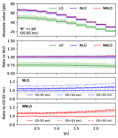
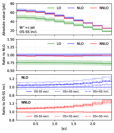
Figure 1: Comparison of predictions for the absolute rapidity of the lepton $|y_{\ell}|$, in the $W^{-}$+$c$-jet (left) and $W^{+}$+$c$-jet (right) processes. Panels from top to bottom: differential distribution at different orders; ratio of differential distributions to NLO; ratio of (OS$-$SS, excl.), (OS+SS, excl.) and (OS+SS, incl.) distributions to (OS$-$SS, incl.) at NLO; same for NNLO.

Figures 1–6 are organised in the following way. On the left we show distributions for $W^{-}$+$c$-jet, on the right for $W^{+}$+$c$-jet. Each column has four panels, depicting: absolute value of the differential distribution at LO, NLO and NNLO in the OS$-$SS incl. setup (1^st panel from the top); ratio of distributions in the OS$-$SS incl. setup at LO, NLO, NNLO to NLO prediction (2^nd panel from the top); ratio of OS$-$SS excl., OS+SS excl. and OS+SS incl. distributions to OS$-$SS incl. distribution at NLO (3^rd panel from the top) and at NNLO (4^th panel from the top).

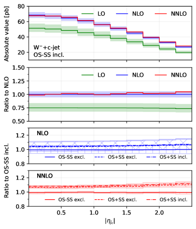
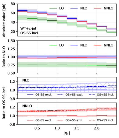
Figure 2: Comparison of predictions for the absolute pseudorapidity of the leading $c$-jet $|\eta_{j_{c}}|$, in the $W^{-}$+$c$-jet (left) and $W^{+}$+$c$-jet (right) processes. Panels from top to bottom: differential distribution at different orders; ratio of differential distributions to NLO; ratio of (OS$-$SS, excl.), (OS+SS, excl.) and (OS+SS, incl.) distributions to (OS$-$SS, incl.) at NLO; same for NNLO.

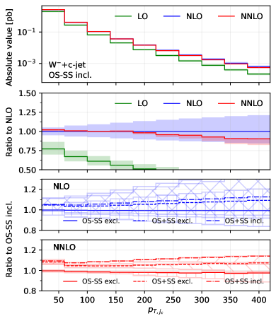
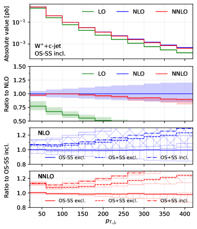
Figure 3: Comparison of predictions for the transverse momentum of the leading $c$-jet $p_{T,j_{c}}$, in the $W^{-}$+$c$-jet (left) and $W^{+}$+$c$-jet (right) processes. Panels from top to bottom: differential distribution at different orders; ratio of differential distributions to NLO; ratio of (OS$-$SS, excl.), (OS+SS, excl.) and (OS+SS, incl.) distributions to (OS$-$SS, incl.) at NLO; same for NNLO.

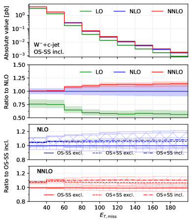
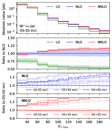
Figure 4: Comparison of predictions for the transverse missing energy $E_{T,{\rm miss}}$, in the $W^{-}$+$c$-jet (left) and $W^{+}$+$c$-jet (right) processes. Panels from top to bottom: differential distribution at different orders; ratio of differential distributions to NLO; ratio of (OS$-$SS, excl.), (OS+SS, excl.) and (OS+SS, incl.) distributions to (OS$-$SS, incl.) at NLO; same for NNLO.

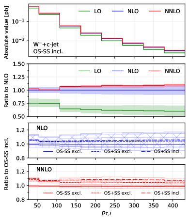
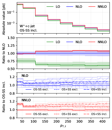
Figure 5: Comparison of predictions for the transverse momentum of the lepton $p_{T,\ell}$, in the $W^{-}$+$c$-jet (left) and $W^{+}$+$c$-jet (right) processes. Panels from top to bottom: differential distribution at different orders; ratio of differential distributions to NLO; ratio of (OS$-$SS, excl.), (OS+SS, excl.) and (OS+SS, incl.) distributions to (OS$-$SS, incl.) at NLO; same for NNLO.

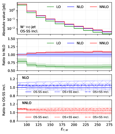
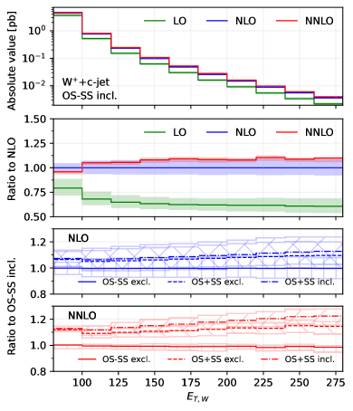
Figure 6: Comparison of predictions for the transverse energy $E_{T,W}$, in the $W^{-}$+$c$-jet (left) and $W^{+}$+$c$-jet (right) processes. Panels from top to bottom: differential distribution at different orders; ratio of differential distributions to NLO; ratio of (OS$-$SS, excl.), (OS+SS, excl.) and (OS+SS, incl.) distributions to (OS$-$SS, incl.) at NLO; same for NNLO.

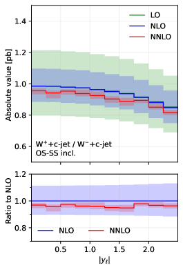
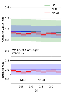
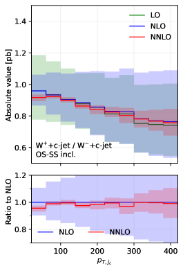
Figure 7: Comparison of differential distributions at different orders for the ratio $\sigma$($W^{+}$+$c$-jet)/$\sigma$($W^{-}$+$c$-jet), differential in $|y_{\ell}|$ (left), $|\eta_{j_{c}}|$ (middle), $p_{T,j_{c}}$ (right). The upper panels show the distributions in absolute value, whereas the lower panels show the ratio to the NLO prediction.

Finally, in Figure 7 we show the distributions differential in $|y_{\ell}|$ (first column), $|\eta_{j_{c}}|$ (second column) and $p_{T,j_{c}}$ (third column), by considering both distributions in absolute value at LO, NLO and NNLO (upper panels) and their ratio to the NLO prediction (lower panels). Here all the predictions are in the OS$-$SS incl. setup.

We first focus on the OS$-$SS incl. setup and we consider predictions at different perturbative orders. We observe in all of the Figures 1–7 a nice perturbative convergence, with the NNLO curves contained within the NLO uncertainty bands, and with the NNLO uncertainty band always smaller by at least a factor of two compared to the NLO one. In the $p_{T,j_{c}}$, $E_{T,{\rm miss}}$, $p_{T,\ell}$ and $E_{T,W}$ distributions, the NNLO curve lies just on the boundary of the NLO uncertainty band. For the ratio $\mathcal{R}^{\pm}_{c}$ in Figure 7, we observe a drastic reduction of the theory uncertainty when moving from LO to NNLO for all the considered distributions, in line with what is observed for the ratio of fiducial cross sections in Section 3.2.

By focussing now on the comparison between different setups, we can draw similar conclusions to those already expressed in Section 3.2. Namely: the difference between excl. and incl. is greater at NNLO than at NLO (remember that at LO all the setups are the same); the difference between excl. and incl. is greater in the OS+SS case rather than in the OS$-$SS case; the difference between OS$-$SS and OS+SS is generally larger than the difference between excl. and incl. However, such differences are generally not flat in the differential distributions. While we observe that the differences between setups mildly depend on $|\eta_{j_{c}}|$, $p_{T,\ell}$ and $E_{T,W}$ for both $W^{+}$+$c$-jet and $W^{-}$+$c$-jet, we note a significant dependence on $|y_{\ell}|$, $p_{T,j_{c}}$ and $E_{T,{\rm miss}}$. In particular, such a dependence is more pronounced at large values of $|y_{\ell}|$, $p_{T,j_{c}}$ and $E_{T,{\rm miss}}$, and the behaviour of $W^{-}$+$c$-jet and $W^{+}$+$c$-jet is very different, with enhanced differences for $W^{+}$+$c$-jet between the different set-ups. We will return to this point in Section 4 below.

We conclude this Section by observing that the difference between excl. and incl. in the OS$-$SS case is very small in all the distributions, both at NLO and NNLO: it amounts to at most a couple of per-cent for high values of $p_{T,j_{c}}$. The OS$-$SS subtraction clearly helps in reducing the difference between the inclusive and exclusive prescription on the number of $c$-jets, because the events discarded when performing the OS$-$SS subtraction are a subset of events with more than one $c$ parton in the event. However, it seems that OS$-$SS subtraction is very efficient in discarding events with more than one $c$-jet surviving the fiducial cuts. In other words, the inclusive two $c$-jets cross section is very small when applying the OS$-$SS subtraction.

4 Partonic channel breakdown

In this section, we study how the individual partonic channels contribute to the total cross section. This analysis will be instrumental in understanding how higher-order radiative corrections in different setups affect the contributions coming from different PDFs.

Figure 8: Born-level diagram for $W^{+}$+$c$-jet and $W^{-}$+$c$-jet.

Figure 9: Example diagrams contributing to $W^{+}$+$c$-jet and $W^{-}$+$c$-jet from NLO onwards.

We recall that at LO, $W+c$-jet production is mediated only through the Born-level process $sg\to W^{-}c$ and $\bar{s}g\to W^{+}\bar{c}$ (Figure 8) and their CKM-suppressed $d$-quark initiated partner processes. They always result in OS final states. At higher orders, final states containing charm quarks can also be caused by a hard scattering process involving an initial-state charm quark or by the splitting of a final state gluon into a charm-anticharm pair, illustrated in Figure 9.

In Tables 4 and 5 we present the contribution of each partonic channel in the $W^{-}$+$c$-jet and in the $W^{+}$+$c$-jet process, respectively. We provide numbers for OS at LO, NLO and NNLO, and for SS at NLO and NNLO (SS at LO is trivially zero). One can easily obtain the corresponding numbers for OS$-$SS and OS+SS. All the numbers refer to exclusive cross sections; the analogous numbers for inclusive cross sections are very similar, so throughout this section we will focus on the exclusive setup (which is more easily interpreted in terms of parton-level subprocesses), unless otherwise specified.

We have chosen to organise the partonic channels in the following way: we explicitly distinguish charm $c$($\bar{c}$) and strange $s$($\bar{s}$) (anti)quarks in the initial state, while denoting an (anti)quark of any other flavour as $q$($\bar{q}$). We do not differentiate between quarks and antiquarks i.e. we sum together contributions coming from quarks and antiquarks of the same flavour. In this way, we obtain 10 possible channels, as listed in the first column of Tables 4 and 5, whose contributions sum up to the total cross section.

$W^{-}$+$c$-jet	OS LO	OS NLO	SS NLO	OS NNLO	SS NNLO
$c(\bar{c})s(\bar{s})$	$0.0$	$-0.1225(3)$	$0.4852(2)$	$-0.05(2)$	$0.842(3)$
$c(\bar{c})c(\bar{c})$	$0.0$	$0.2158(1)$	$0.2062(2)$	$0.360(2)$	$0.351(1)$
$c(\bar{c})q(\bar{q})$	$0.0$	$1.2392(3)$	$1.3132(4)$	$1.958(4)$	$2.088(4)$
$s(\bar{s})q(\bar{q})$	$0.0$	$-0.651(3)$	$0.03134(1)$	$-1.1(2)$	$0.0537(2)$
$s(\bar{s})s(\bar{s})$	$0.0$	$-0.2549(3)$	$0.0$	$-0.42(3)$	$0.0$
$q(\bar{q})q(\bar{q})$	$0.0$	$1.0314(7)$	$0.9838(4)$	$1.73(2)$	$1.676(6)$
$gq(\bar{q})$	$8.9255(6)$	$12.700(1)$	$0.0$	$12.7(2)$	$0.405(3)$
$gs(\bar{s})$	$86.857(4)$	$123.002(8)$	$0.0$	$128.9(3)$	$-0.0353(6)$
$gc(\bar{c})$	$0.0$	$0.0$	$0.0$	$-0.14(2)$	$-0.057(2)$
$gg$	$0.0$	$-6.355(3)$	$0.0$	$-8.31(1)$	$0.0$
total	$95.782(5)$	$130.806(1)$	$3.020(1)$	$135.6(5)$	$5.324(9)$

Table 4: Breakdown of the fiducial cross section for $W^{-}$+$c$-jet in terms of the contributing partonic channels. We denote as $q(\bar{q})$ the quarks (antiquarks) of different flavour than $s(\bar{s})$ and $c(\bar{c})$. Furthermore, we do not distinguish between quarks and antiquarks e.g. the $c(\bar{c})s(\bar{s})$ row contains all the possible permutations of $c$ and $\bar{c}$ with $s$ and $\bar{s}$. All the numbers refer to exclusive cross sections.

$W^{+}$+$c$-jet	OS LO	OS NLO	SS NLO	OS NNLO	SS NNLO
$c(\bar{c})s(\bar{s})$	$0.0$	$-0.1191(9)$	$0.4752(4)$	$-0.13(2)$	$0.838(1)$
$c(\bar{c})c(\bar{c})$	$0.0$	$0.2151(3)$	$0.2047(3)$	$0.3316(5)$	$0.3246(6)$
$c(\bar{c})q(\bar{q})$	$0.0$	$1.948(3)$	$1.988(4)$	$2.945(6)$	$3.038(6)$
$s(\bar{s})q(\bar{q})$	$0.0$	$-0.649(9)$	$0.0673(1)$	$-1.9(3)$	$0.1157(3)$
$s(\bar{s})s(\bar{s})$	$0.0$	$-0.258(1)$	$0.0$	$-0.55(5)$	$0.0$
$q(\bar{q})q(\bar{q})$	$0.0$	$1.431(2)$	$1.409(2)$	$2.35(2)$	$2.423(6)$
$gq(\bar{q})$	$5.8299(7)$	$8.257(2)$	$0.0$	$10.1(4)$	$0.508(4)$
$gs(\bar{s})$	$85.51(1)$	$121.04(3)$	$0.0$	$126.3(6)$	$-0.0430(4)$
$gc(\bar{c})$	$0.0$	$0.0$	$0.0$	$0.02(2)$	$-0.0293(7)$
$gg$	$0.0$	$-6.34(1)$	$0.0$	$-13.62(6)$	$0.0$
total	$91.34(1)$	$125.51(4)$	$4.146(4)$	$125.9(7)$	$7.17(1)$

Table 5: Breakdown of the fiducial cross section for $W^{+}$+$c$-jet in terms of the contributing partonic channels. As in Table 4 we denote as $q(\bar{q})$ the quarks (antiquarks) of different flavour than $s(\bar{s})$ and $c(\bar{c})$. Furthermore, we do not distinguish between quarks and antiquarks e.g. the $c(\bar{c})s(\bar{s})$ row contains all the possible permutations of $c$ and $\bar{c}$ with $s$ and $\bar{s}$. All the numbers refer to exclusive cross sections.

At all perturbative orders, the by far dominant contribution to the fiducial cross section in OS events comes from the $gs(\bar{s})$ channel, which amounts to 90% of the total. The second largest contribution (6–10%) to OS events comes from the $gq(\bar{q})$ channel. Such a contribution is slightly larger for $W^{-}$+$c$-jet: as already explained in Section 3.2, this is related to the presence of the $d$ PDF in $W^{-}$+$c$-jet as opposed to the presence of $\bar{d}$ in $W^{+}$+$c$-jet. The third largest contribution (5–10%) comes from the $gg$ channel, with a negative sign, partially compensating the $gq(\bar{q})$ contribution. In some cases, the $gg$ channel can be even larger than the $gq(\bar{q})$ one (for instance in $W^{+}$+$c$-jet for OS at NNLO). All the other channels contribute much less to the total cross section (at most a few per-cent each).

It is interesting to compare the OS numbers for some channels with the analogous ones for SS. We notice that both at NLO and at NNLO, both for $W^{+}$+$c$-jet and for $W^{-}$+$c$-jet, the $c(\bar{c})c(\bar{c})$ channel, the $c(\bar{c})q(\bar{q})$ channel and the $q(\bar{q})q(\bar{q})$ channel are numerically very similar between OS and SS. Hence when performing the OS$-$SS subtraction, we are enhancing the channels featuring a (anti)strange PDF, by removing channels with quarks of other flavours. The channels with a gluon PDF ($gq(\bar{q})$ and $gg$) still survive after the OS$-$SS subtraction.

In order to investigate how the overall picture is affected by different kinematical regions of phase space, we also investigate selected differential distributions. We focus on the $|y_{\ell}|$ and $p_{T,j_{c}}$ observables, and we consider the fractional contribution of each individual channel at each perturbative order for each bin of the corresponding differential distributions. The results are shown in Figure 10 ($|y_{\ell}|$ in $W^{-}$+$c$-jet), Figure 11 ($|y_{\ell}|$ in $W^{+}$+$c$-jet), Figure 12 ($p_{T,j_{c}}$ in $W^{-}$+$c$-jet) and Figure 13 ($p_{T,j_{c}}$ in $W^{+}$+$c$-jet). In each figure, we plot the contribution of each partonic channel normalised to the total at LO (1${}^{\text{st}}$ row from the top), total NLO (2${}^{\text{nd}}$ row from the top) and total NNLO (3${}^{\text{rd}}$ row from the top). The left and the middle columns are in the OS$-$SS excl. and OS+SS excl. setups, respectively, whereas the right column is in the SS setup. We chose to plot OS$-$SS excl. and OS+SS excl.  in order to have a complementary information to the one provided in Tables 4–5. Instead, in the SS column, one can better appreciate the difference between the several curves, given that the dominant $gs(\bar{s})$ component is absent.

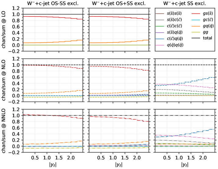
Figure 10: Fractional contribution of partonic channels to the total result at different perturbative orders, for the $W^{-}$+$c$-jet process, differential in $|y_{\ell}|$. The three columns correspond to different setups: OS$-$SS excl. (left), OS+SS excl. (middle), SS excl. (right). The three rows correspond to different perturbative orders: LO (top), NLO (middle), NNLO (bottom).

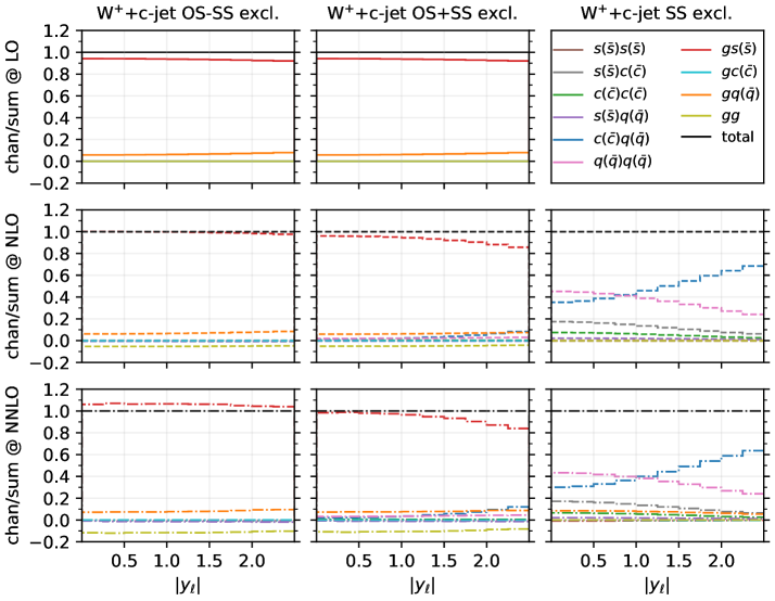
Figure 11: Fractional contribution of partonic channels to the total result at different perturbative orders, for the $W^{+}$+$c$-jet process, differential in $|y_{\ell}|$. The three columns correspond to different setups: OS$-$SS excl. (left), OS+SS excl. (middle), SS excl. (right). The three rows correspond to different perturbative orders: LO (top), NLO (middle), NNLO (bottom).

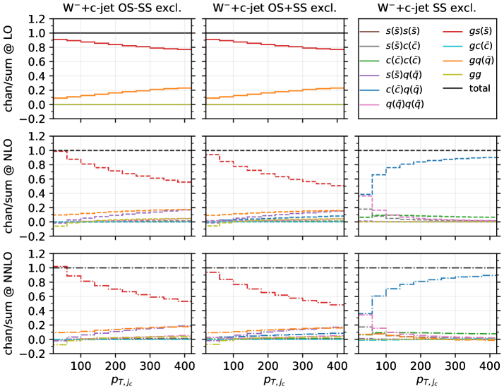
Figure 12: Fractional contribution of partonic channels to the total result at different perturbative orders, for the $W^{-}$+$c$-jet process, differential in $p_{T,j_{c}}$. The three columns correspond to different setups: OS$-$SS excl. (left), OS+SS excl. (middle), SS excl. (right). The three rows correspond to different perturbative orders: LO (top), NLO (middle), NNLO (bottom).

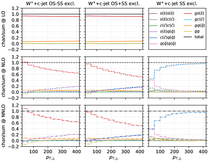
Figure 13: Fractional contribution of partonic channels to the total result at different perturbative orders, for the $W^{+}$+$c$-jet process, differential in $p_{T,j_{c}}$. The three columns correspond to different setups: OS$-$SS excl. (left), OS+SS excl. (middle), SS excl. (right). The three rows correspond to different perturbative orders: LO (top), NLO (middle), NNLO (bottom).

We first focus on the OS$-$SS excl. and OS+SS excl. setups. In all plots, we notice the dominance of the $gs(\bar{s})$ channel, as already observed for the fiducial cross sections. However, it can be seen that for large values of $|y_{\ell}|$ and $p_{T,j_{c}}$, the fractional contribution of $gs(\bar{s})$ decreases, with the other channels starting to contribute more. In particular, in the $|y_{\ell}|$ distribution, we observe that $gs(\bar{s})$ is always very close to 1 for most of the rapidity range, except for $|y_{\ell}|\gtrsim 2.0$ where it decreases to 0.8. The overall picture is only mildly affected by the perturbative order. In contrast, in the $p_{T,j_{c}}$ distribution, we note a sharp decrease of the $gs(\bar{s})$ contribution as $p_{T,j_{c}}$ increases: while at LO $gs(\bar{s})$ is around 0.9 for low-$p_{T,j_{c}}$ values down to 0.8 for high-$p_{T,j_{c}}$ values, at NLO and NNLO it goes down to 0.5–0.6 for $p_{T,j_{c}}\sim 400$ GeV. Other channels then give a non-negligible contribution at high transverse momenta: the $gq(\bar{q})$ and $s(\bar{s})q(\bar{q})$ channels both in the OS$-$SS and OS+SS setup; the $c(\bar{c})q(\bar{q})$ channels only in the OS+SS setup. Indeed, by comparing left columns (OS$-$SS) with the middle columns (OS+SS), the effect of the OS$-$SS subtraction is evident, with the curve associated to $c(\bar{c})q(\bar{q})$ close to zero on the left. As for the $gg$ channel, its contribution mildly depends on $|y_{\ell}|$, being negative and constant in the whole rapidity range. Instead, it peaks at low-$p_{T,j_{c}}$ at NLO and NNLO (where the total cross section is larger), with a negligible contribution at large transverse momenta.

It is also interesting to note how the individual channels behave between $W^{-}$+$c$-jet and $W^{+}$+$c$-jet. For instance, already at LO, the behaviour of the $gq(\bar{q})$ channel both at large rapidities and at large transverse momenta is different, with a larger contribution of $gq(\bar{q})$ in $W^{-}$+$c$-jet. These kinematic regions mainly receive contributions from PDFs at large momentum fraction; hence, the plots confirm that the origin of the difference between $W^{-}$+$c$-jet and $W^{+}$+$c$-jet to be related to the valence component of the $d$ PDF, which is absent for the $\bar{d}$ PDF. Equally noteworthy is the difference in size between the $c(\bar{c})q(\bar{q})$ and the $q(\bar{q})q(\bar{q})$ channels in $W^{+}$+$c$-jet and $W^{-}$+$c$-jet at NLO and NNLO in the OS+SS excl. setup.

We now consider the SS plots i.e. the column on the right in Figs. 10–13. We see that both $c(\bar{c})q(\bar{q})$ and $q(\bar{q})q(\bar{q})$ are equally dominant for small rapidity values, with $c(\bar{c})q(\bar{q})$ becoming larger and $q(\bar{q})q(\bar{q})$ becoming smaller at large rapidities, both at NLO and NNLO. The situation is similar in the $p_{T,j_{c}}$ distribution, but starting from $p_{T,j_{c}}\gtrsim 300$ GeV the $c(\bar{c})q(\bar{q})$ channel constitutes the totality of the SS cross section, with the $q(\bar{q})q(\bar{q})$ near to zero. It is likely that in these events at large-$p_{T,j_{c}}$ the SS $c$-parton comes directly from the PDFs: if it were radiatively generated, then other channels would also contribute.

Having scrutinized in detail how contributions to the cross sections are distributed among the various channels, we now return to consider the bottom panels of Fig. 3. Namely, understanding why the behaviour of the considered setups is so different between $W^{-}$+$c$-jet and $W^{+}$+$c$-jet in the $p_{T,j_{c}}$ distribution. This will give us the opportunity to further investigate the correlation between PDFs and cross sections for $W^{-}$+$c$-jet and $W^{+}$+$c$-jet.

Towards this aim, we consider again the $p_{T,j_{c}}$ distribution at NLO (Figure 14) and at NNLO (Figure 15). However we now include curves with the contributions of the most sizeable channels, and superimpose $W^{+}$+$c$-jet and $W^{-}$+$c$-jet on the same plot, by choosing as common normalisation factor the $W^{-}$+$c$-jet OS$-$SS incl. distribution. In this way, we can determine the relative size of contributions between $W^{+}$+$c$-jet and $W^{-}$+$c$-jet. The darker colours refer to $W^{-}$+$c$-jet, whereas the lighter ones to $W^{+}$+$c$-jet. We show results for the OS$-$SS excl. setup (left frames), the OS+SS excl. setup (middle frames), the OS+SS incl. setup (right frames). The black curves in the upper left plots of Figures 14 and 15 coincide with the blue (NLO) and red (NNLO) curves in the left plot in Fig. 3. Likewise, the gray curves in the upper left plots of Figures 14 and 15 correspond to the blue and red curves in the right plot in Fig. 3, but they do not coincide as they have a different normalisation.

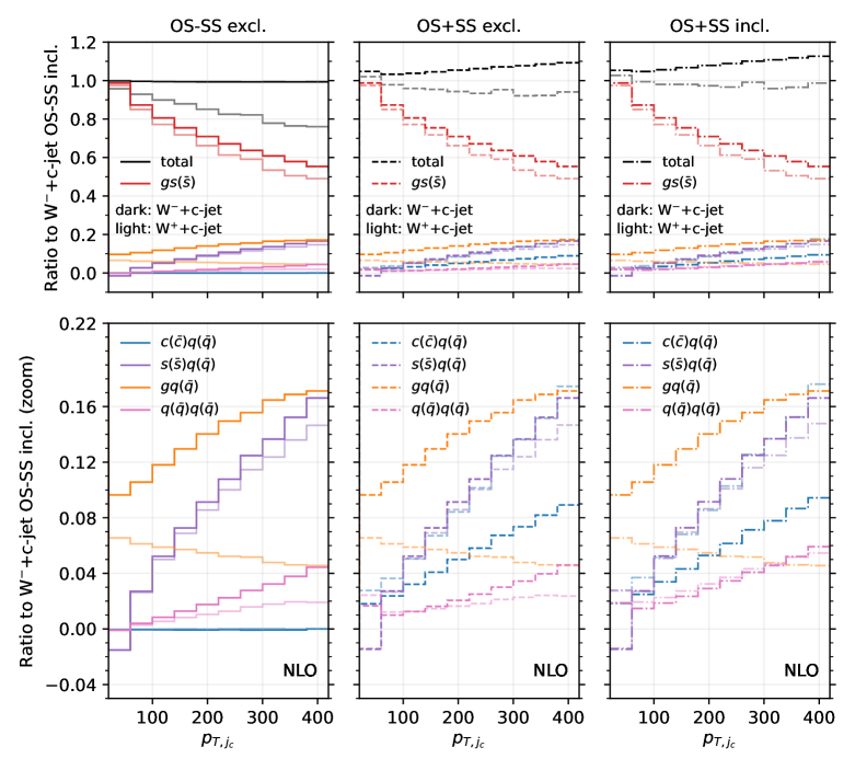
Figure 14: Analysis of the channels contributing to the $p_{T,j_{c}}$ distribution at NLO for OS$-$SS excl.(left), OS+SS excl.(middle) and OS+SS incl.(right). All the curves are normalised to the $W^{-}$+$c$-jet OS$-$SS incl. NLO distribution. The lower panel is just a zoom of the upper panel. Darker colours refer to $W^{-}$+$c$-jet, lighter colours refer to $W^{+}$+$c$-jet.

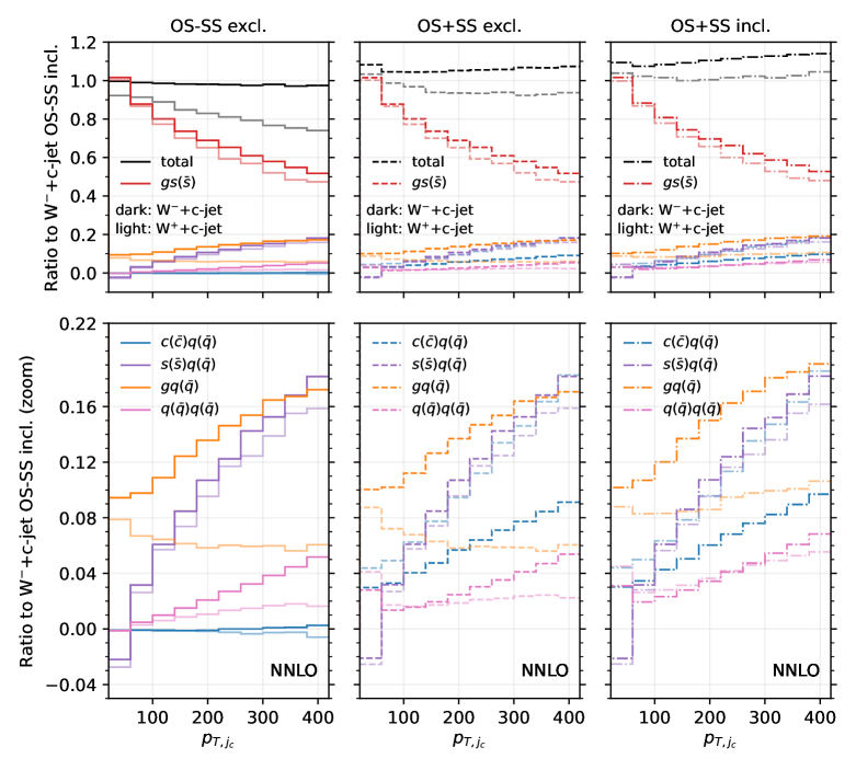
Figure 15: Analysis of the channels contributing to the $p_{T,j_{c}}$ distribution at NNLO for OS$-$SS excl.(left), OS+SS excl.(middle) and OS+SS incl.(right). All the curves are normalised to the $W^{-}$+$c$-jet OS$-$SS incl. NLO distribution. The lower panel is just a zoom of the upper panel. Darker colours refer to $W^{-}$+$c$-jet, lighter colours refer to $W^{+}$+$c$-jet.

We observe several important features. At NLO for both $W^{-}$+$c$-jet and $W^{+}$+$c$-jet, the difference between OS+SS excl. and OS$-$SS excl. is driven by the $c(\bar{c})q(\bar{q})$ channel, and the difference between OS+SS excl. and OS+SS incl. is driven by $q(\bar{q})q(\bar{q})$. At NNLO, similar observations hold, with $gq(\bar{q})$ channel responsible for further increasing the difference between OS+SS excl. and OS+SS incl. Hence, explaining the lower panels of Fig. 3 amounts to understanding why the $c(\bar{c})q(\bar{q})$, $q(\bar{q})q(\bar{q})$ and $gq(\bar{q})$ channels are so different in size between $W^{-}$+$c$-jet and $W^{+}$+$c$-jet.

Starting from the $c(\bar{c})q(\bar{q})$ channel, from the discussion above we know that in the high-$p_{T,j_{c}}$ region these events feature a SS $c$-parton coming directly from the PDFs. Therefore, the quark line coupling to the $W$-boson is unconstrained in terms of flavour. A typical diagram of such a configuration is displayed in Figure 9 on the left. The largest contribution in the large-$x$ region comes from the $d$ valence PDF in the case of $W^{-}$ and from the $u$ valence PDF in the case of $W^{+}$. The latter is approximately twice of the former, hence the factor of roughly 2 between the contribution of the $c(\bar{c})q(\bar{q})$ channel in OS+SS for $W^{-}$+$c$-jet and for $W^{+}$+$c$-jet in the large-$p_{T,j_{c}}$ region is easily explained.

One can explain in a similar manner why the $q(\bar{q})q(\bar{q})$ and $gq(\bar{q})$ channels induce the difference between the incl. and the excl. setup, and why such a difference is greater for $W^{+}$+$c$-jet compared to $W^{-}$+$c$-jet. A typical diagram for $q(\bar{q})q(\bar{q})$ is shown in Fig. 9 on the right. In this case, the charm is generated radiatively, hence we are summing over the flavour combinations of the two incoming quarks. Again the largest contributions in the large-$x$ region comes from the $u\bar{d}$ channel in $W^{+}$+$c$-jet and from the $d\bar{u}$ channel in $W^{-}$+$c$-jet, so one recover the factor of 2 in difference. Similar considerations apply to the $gq(\bar{q})$ channels, which however features a secondary pair of charm quarks only starting from NNLO.

5 Conclusions

In this paper, we presented a new calculation of $W$+charm-jet production up to NNLO in QCD. We employed a new flavour-dressing procedure Gauld:2022lem to define charm-jets in an IRC safe manner. Our results confirm an earlier calculation Czakon:2020coa ; Czakon:2022khx , applied to the kinematics of a recent CMS measurement CMS:2023aim . A detailed decomposition into different partonic channels demonstrated that the predominant contribution from initial states containing strange quarks is maintained in most kinematical distributions even when higher-order corrections are included. The efficiency of the OS$-$SS subtraction in removing contributions from secondary charm production is clearly demonstrated by the channel decomposition. This decomposition also explains the consistently larger magnitude of the $W^{-}$+$c$-jet over $W^{+}$+$c$-jet cross sections to be due to contributions from CKM-suppressed $d$-valence quark initiated processes.

Our results demonstrate the practical application of flavour dressing Gauld:2022lem in NNLO QCD predictions. They will enable the usage of $W$+charm-jet production observables in future global NNLO PDF fits and thus enable a precise flavour composition of the quark content of the nucleon.

- (1) G. Altarelli and G. Parisi, Asymptotic Freedom in Parton Language, Nucl. Phys. B 126 (1977) 298.
- (2) Y.L. Dokshitzer, Calculation of the Structure Functions for Deep Inelastic Scattering and Annihilation by Perturbation Theory in Quantum Chromodynamics., Sov. Phys. JETP 46 (1977) 641.
- (3) J. Gao, L. Harland-Lang and J. Rojo, The Structure of the Proton in the LHC Precision Era, Phys. Rept. 742 (2018) 1 [1709.04922].
- (4) S. Alekhin, J. Blümlein, S. Moch and R. Placakyte, Parton distribution functions, , and heavy-quark masses for LHC Run II, Phys. Rev. D 96 (2017) 014011 [1701.05838].
- (5) T.-J. Hou et al., New CTEQ global analysis of quantum chromodynamics with high-precision data from the LHC, Phys. Rev. D 103 (2021) 014013 [1912.10053].
- (6) S. Bailey, T. Cridge, L.A. Harland-Lang, A.D. Martin and R.S. Thorne, Parton distributions from LHC, HERA, Tevatron and fixed target data: MSHT20 PDFs, Eur. Phys. J. C 81 (2021) 341 [2012.04684].
- (7) NNPDF collaboration, The path to proton structure at 1% accuracy, Eur. Phys. J. C 82 (2022) 428 [2109.02653].
- (8) CTEQ collaboration, CTEQ parton distributions and flavor dependence of sea quarks, Phys. Lett. B 304 (1993) 159 [hep-ph/9303255].
- (9) NuTeV collaboration, Precise measurement of neutrino and anti-neutrino differential cross sections, Phys. Rev. D 74 (2006) 012008 [hep-ex/0509010].
- (10) U. Baur, F. Halzen, S. Keller, M.L. Mangano and K. Riesselmann, The Charm content of + 1 jet events as a probe of the strange quark distribution function, Phys. Lett. B 318 (1993) 544 [hep-ph/9308370].
- (11) W.T. Giele, S. Keller and E. Laenen, QCD corrections to boson plus heavy quark production at the Tevatron, Phys. Lett. B 372 (1996) 141 [hep-ph/9511449].
- (12) W.J. Stirling and E. Vryonidou, Charm production in association with an electroweak gauge boson at the LHC, Phys. Rev. Lett. 109 (2012) 082002 [1203.6781].
- (13) M. Czakon, A. Mitov, M. Pellen and R. Poncelet, NNLO QCD predictions for +-jet production at the LHC, JHEP 06 (2021) 100 [2011.01011].
- (14) M. Czakon, A. Mitov, M. Pellen and R. Poncelet, A detailed investigation of W+c-jet at the LHC, JHEP 02 (2023) 241 [2212.00467].
- (15) ATLAS collaboration, Measurement of the production of a boson in association with a charmed hadron in collisions at with the ATLAS detector, Phys. Rev. D 108 (2023) 032012 [2302.00336].
- (16) CMS collaboration, Measurement of Associated + Charm Production in pp Collisions at = 7 TeV, JHEP 02 (2014) 013 [1310.1138].
- (17) CMS collaboration, Measurements of the associated production of a W boson and a charm quark in proton–proton collisions at , Eur. Phys. J. C 82 (2022) 1094 [2112.00895].
- (18) CMS collaboration, Measurement of the production cross section for a W boson in association with a charm quark in proton-proton collisions at = 13 TeV, 2308.02285.
- (19) LHCb collaboration, Study of boson production in association with beauty and charm, Phys. Rev. D 92 (2015) 052001 [1505.04051].
- (20) A. Banfi, G.P. Salam and G. Zanderighi, Infrared safe definition of jet flavor, Eur. Phys. J. C 47 (2006) 113 [hep-ph/0601139].
- (21) S. Caletti, A.J. Larkoski, S. Marzani and D. Reichelt, Practical jet flavour through NNLO, Eur. Phys. J. C 82 (2022) 632 [2205.01109].
- (22) M. Czakon, A. Mitov and R. Poncelet, Infrared-safe flavoured anti-kT jets, JHEP 04 (2023) 138 [2205.11879].
- (23) R. Gauld, A. Huss and G. Stagnitto, Flavor Identification of Reconstructed Hadronic Jets, Phys. Rev. Lett. 130 (2023) 161901 [2208.11138].
- (24) F. Caola, R. Grabarczyk, M.L. Hutt, G.P. Salam, L. Scyboz and J. Thaler, Flavored jets with exact anti-kT kinematics and tests of infrared and collinear safety, Phys. Rev. D 108 (2023) 094010 [2306.07314].
- (25) G. Bevilacqua, M.V. Garzelli, A. Kardos and L. Toth, W + charm production with massive c quarks in PowHel, JHEP 04 (2022) 056 [2106.11261].
- (26) S. Ferrario Ravasio and C. Oleari, NLO + parton-shower generator for Wc production in the POWHEG BOX RES, Eur. Phys. J. C 83 (2023) 684 [2304.13791].
- (27) A. Gehrmann-De Ridder, T. Gehrmann, E.W.N. Glover, A. Huss and T.A. Morgan, Precise QCD predictions for the production of a boson in association with a hadronic jet, Phys. Rev. Lett. 117 (2016) 022001 [1507.02850].
- (28) A. Gehrmann-De Ridder, T. Gehrmann and E.W.N. Glover, Antenna subtraction at NNLO, JHEP 09 (2005) 056 [hep-ph/0505111].
- (29) A. Daleo, T. Gehrmann and D. Maitre, Antenna subtraction with hadronic initial states, JHEP 04 (2007) 016 [hep-ph/0612257].
- (30) J. Currie, E.W.N. Glover and S. Wells, Infrared Structure at NNLO Using Antenna Subtraction, JHEP 04 (2013) 066 [1301.4693].
- (31) A. Gehrmann-De Ridder, T. Gehrmann, E.W.N. Glover, A. Huss and D.M. Walker, Next-to-Next-to-Leading-Order QCD Corrections to the Transverse Momentum Distribution of Weak Gauge Bosons, Phys. Rev. Lett. 120 (2018) 122001 [1712.07543].
- (32) A. Gehrmann-De Ridder, T. Gehrmann, E.W.N. Glover, A. Huss and D.M. Walker, Vector Boson Production in Association with a Jet at Forward Rapidities, Eur. Phys. J. C 79 (2019) 526 [1901.11041].
- (33) L.W. Garland, T. Gehrmann, E.W.N. Glover, A. Koukoutsakis and E. Remiddi, The Two loop QCD matrix element for jets, Nucl. Phys. B 627 (2002) 107 [hep-ph/0112081].
- (34) L.W. Garland, T. Gehrmann, E.W.N. Glover, A. Koukoutsakis and E. Remiddi, Two loop QCD helicity amplitudes for three jets, Nucl. Phys. B 642 (2002) 227 [hep-ph/0206067].
- (35) E.W.N. Glover and D.J. Miller, The One loop QCD corrections for , Phys. Lett. B 396 (1997) 257 [hep-ph/9609474].
- (36) J.M. Campbell, E.W.N. Glover and D.J. Miller, The One loop QCD corrections for , Phys. Lett. B 409 (1997) 503 [hep-ph/9706297].
- (37) Z. Bern, L.J. Dixon and D.A. Kosower, One loop amplitudes for to four partons, Nucl. Phys. B 513 (1998) 3 [hep-ph/9708239].
- (38) K. Hagiwara and D. Zeppenfeld, Amplitudes for Multiparton Processes Involving a Current at , , and Hadron Colliders, Nucl. Phys. B 313 (1989) 560.
- (39) F.A. Berends, W.T. Giele and H. Kuijf, Exact Expressions for Processes Involving a Vector Boson and Up to Five Partons, Nucl. Phys. B 321 (1989) 39.
- (40) R. Gauld, A. Gehrmann-De Ridder, E.W.N. Glover, A. Huss and I. Majer, Predictions for -Boson Production in Association with a -Jet at , Phys. Rev. Lett. 125 (2020) 222002 [2005.03016].
- (41) R. Gauld, A. Gehrmann-De Ridder, E.W.N. Glover, A. Huss, A.R. Garcia and G. Stagnitto, NNLO QCD predictions for Z-boson production in association with a charm jet within the LHCb fiducial region, Eur. Phys. J. C 83 (2023) 336 [2302.12844].
- (42) R. Gauld, A. Gehrmann-De Ridder, E.W.N. Glover, A. Huss and I. Majer, Associated production of a Higgs boson decaying into bottom quarks and a weak vector boson decaying leptonically at NNLO in QCD, JHEP 10 (2019) 002 [1907.05836].
- (43) S. Catani and M.H. Seymour, A General algorithm for calculating jet cross-sections in NLO QCD, Nucl. Phys. B 485 (1997) 291 [hep-ph/9605323].
- (44) M. Cacciari, G.P. Salam and G. Soyez, The anti- jet clustering algorithm, JHEP 04 (2008) 063 [0802.1189].
- (45) PDF4LHC Working Group collaboration, The PDF4LHC21 combination of global PDF fits for the LHC Run III, J. Phys. G 49 (2022) 080501 [2203.05506].
- (46) A. Buckley, J. Ferrando, S. Lloyd, K. Nordström, B. Page, M. Rüfenacht et al., LHAPDF6: parton density access in the LHC precision era, Eur. Phys. J. C75 (2015) 132 [1412.7420].
- (47) Particle Data Group collaboration, Review of Particle Physics, PTEP 2020 (2020) 083C01.
- (48) E.W.N. Glover and J. Pires, Antenna subtraction for gluon scattering at NNLO, JHEP 06 (2010) 096 [1003.2824].