Adaptive time delay based control of non-collocated oscillatory systems

Abstract

Time delay based control, recently proposed for non-collocated fourth-order systems, has several advantages over an observer-based state-feedback cancelation of the low-damped oscillations of the output. In this paper, we discuss a practical infeasibility of such observer-based approach and bring forward the application of the time delay based controller, which is simple in both the structure and design. A robust estimation of the output oscillation frequency is used and extended, in this work, by a bias cancelation that is required for tracking the oscillatory load. This way, an adaptive tuning of the time delay based controller is realized which does not require knowledge of the mass and stiffness parameters. The results are demonstrated on the oscillatory experimental setup with constraints in both the operation range and control value.

I Introduction

Multi-mass systems with an oscillatory passive load are common in various control applications. A broad class of such systems can be approximated by fourth-order dynamics where the first active body includes the whole actuator plant, while the second passive body represents the whole oscillating payload to be controlled. Elastic links, especially when with low damping, make such systems challenging for stabilization. Moreover, if only the load output state is available from the sensor measurements, such systems become non-collocated – that is the objective of our present study. For instance in cranes (see e.g. [1]) and winch systems, the vertical oscillation dynamics can become essential, due to the elasticities in ropes and cables. Longitudinal oscillations in hoisting systems (see e.g. [2]) are known to be complex, so that the output oscillation frequency becomes highly uncertain and valid only close to an operation point. Also the drill-string systems, for instance, represent a case of oscillatory passive loads (with angular motion), see e.g. [3], while such vibration dynamics becomes rather non-trivial.

In this work, we consider a class of fourth-order non-collocated oscillation systems (Section II), for which stabilization only a noisy sensing of the load output displacement is available. We first discuss in detail a practical infeasibility of the classical observer-based state-feedback design with loop reshaping by the poles location (Section III). We demonstrate that even a low measurement noise, in combination with constraints of the actuator’s force and displacement, makes such a theoretically sound stabilization less usable. Then, it is shown (in Section IV) that the recently proposed time delay based control [4, 5] constitutes a suitable robust alternative for such class of the systems. Also, an adaptive online tuning of the oscillation frequency, required for the controller parametrization, is provided while extending the robust estimator [5]. The design of the time delay based stabilization is simple and relies on system characteristics in frequency domain. Here we recall that analysis of systems with time delay(s) is manageable also with use of the corresponding transfer functions, see [6]. For signal-norms analysis of the systems with time delays it is referred to [7]. For tutorial and backgrounds on the time-delay systems we also refer to [8, 9, 10]. Experimental evaluation of the proposed control is reported in Section V, with the adaptive frequency tuning and also additional external disturbances.

II Non-collocated fourth-order system

II-A General framework

We consider a general framework of the non-collocated fourth-order systems, as schematically depicted in Fig. 1. The system has an active and a passive body with the mass $m$ and $M$, correspondingly. The relative motion is actuated by the constrained force $f\in[f_{\min},f_{\max}]$ and has one degree of freedom in the shifted (against each other) coordinates $(z,\dot{z})$ and $(y,\dot{y})$.

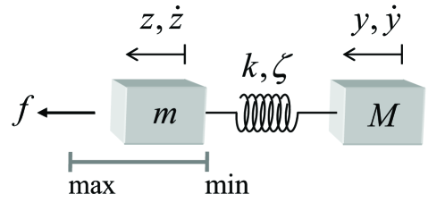
Figure 1: General framework of non-collocated system.

Both inertial bodies are connected by an elastic link (i.e. spring), with the linear stiffness and damping coefficients $k$ and $\zeta$, respectively. In addition, the first active body can be subject to the linear damping $\sigma$ (equivalent to the viscous friction of an actuator), while the second passive body can be low-damped or even undamped, – a challenging case we study (also with experiments) in this work. Both moving bodies can be additionally affected by the known constant (or slowly varying) disturbances $\varphi$ and $\Phi$, each one individually. Further essential assumption is that the active mass has a constrained motion range

$$z\in(z_{\min},z_{\max}),$$ (1)

the fact which is often occurring due to the mechanical limiters of an actuator. With the above assumptions, the motion dynamics within displacement range (1) is given by

$$m\ddot{z}+(\sigma+\zeta)\,\dot{z}+k(z-y)-\zeta\dot{y}+\varphi = f,$$ (2)

$$M\ddot{y}-\zeta(\dot{z}-\dot{y})-k(z-y)+\Phi = 0.$$ (3)

The link damping $\zeta>0$ is assumed to be relatively low, so that the load motion of an uncontrolled system experiences a long-term oscillatory (and parasitic for applications) behavior, in the $(y,\dot{y})$ coordinates. One of the most challenging (for regulation) characteristics of the system class (2), (3) is the non-collocation of the control value $f$ and the available output of interest $y$. Note that $y(t)$ is the single measurable system state, which can additionally be corrupted by the sensor noise. Furthermore, we note that all trajectories in the four-dimensional state-space of (2), (3) are continuous and smooth within (1), while for $z=z_{\min}\vee z_{\max}$ the switchings appear, see e.g. [11] for fundamentals of the switched dynamics. This is especially relevant for a constrained motion, addressed later in sections II-B, III-B as a factor limiting the performance and feasibility of the control.

II-B Experimental case study

The present experimental case study is a non-collocated fourth-order system under gravity, with a contactless output sensing, see Fig. 2. The actuated active body is the voice-coil-motor with the bounded input and output

$$u\in[0,\,10]\hbox{ V,}\quad\hbox{ and }\quad z\in[0,\,0.021]\hbox{ m,}$$

respectively. An additional actuator’s time constant yields

$$f(s)=F(s)u(s)=\frac{\kappa}{\tau s+1}\,u(s)=\frac{3.2811}{0.0012s+1}\,u(s),$$ (4)

written in Laplace domain with the complex variable $s$. The relative displacement of the passive load is measured contactless by an inductive distance sensor, which has $\pm 12$ $\mu m$ nominal repeatability and a relatively large level of noise. The latter is due to contactless measurement and dynamic misalignments of the moving body with respect to the inductive field cone of the sensor. Here recall that there is no bearing for the load mass which is, this way, constituting a free-hanging body, see Fig. 2. Further details about the experimental system can be looked in [12, 5].

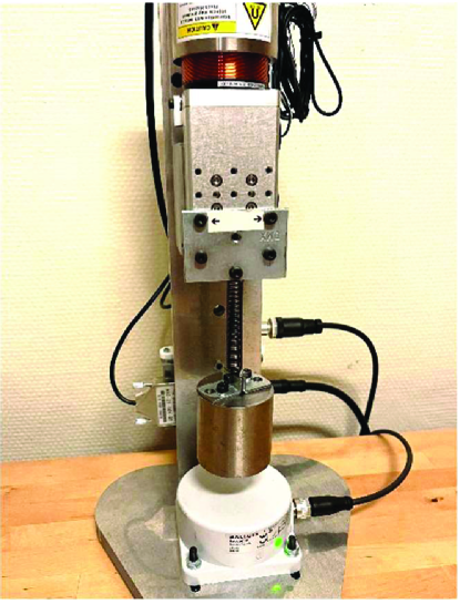
Figure 2: Experimental setup of non-collocated system.

For the vector of state variables $x\equiv(x_{1},x_{2},x_{3},x_{4})^{\top}=(\dot{z},z,\dot{y},y)^{\top}$, the state-space model, corresponding to (2), (3), is given by

$$\dot{x} = A\,x+B\,f+D,$$ (5)

$$y = C\,x,$$

with

$$A = \left(\begin{array}[]{cccc}-333.35&-333.33&0.015&333.33\\ 1&0&0&0\\ 0.012&266.66&-0.012&-266.66\\ 0&0&1&0\end{array}\right),$$ (10)

$$B = (1.667,0,0,0)^{\top},\quad C\;=\;(0,0,0,1),\;\hbox{ and}$$

$$D = (-9.806,0,-9.806,0)^{\top}.$$

Worth noting is that the disturbance vector $D$, cf. (2), (3), is composed by the constant gravity terms acting on both moving bodies. Further we emphasize that the system (5) has one conjugate-complex pole-pair with the natural frequency $\omega_{0}=16.4$ rad/sec and an extremely low damping ratio $\delta=0.031$. The numerical parameter values of the system model were identified, partially from the available technical data-sheets of components and partially through a series of dedicated experiments, cf. [4, 13]. An exemplary comparison between the measured and modeled output response is shown in Fig. 3 for a free fall scenario. It means that starting from non-zeros initial conditions and having $u(t)=\mathrm{const}$ for the gravity compensation, the control input is then switched off at $t=20$ sec. This leads to $u(t)=0$ for $t>20$ and a fall down of both masses, while $|\dot{z}|<|\dot{y}|$ due to the actuator bearing. Hence, the oscillatory behavior becomes largely excited once $z=z_{\min}$.

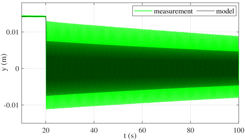
Figure 3: Comparison of measured and computed oscillatory response of free fall scenario ($f(t)=0$ for $t>20$ s).

Note that while the the oscillation frequency $\omega=\omega_{0}\sqrt{1-\delta^{2}}$, damping ratio $\delta$, and the steady-sate values of $y(t)$ are well in accord between the measurement and model, the oscillations amplitude is sensitive to both, the initial conditions and exact knowledge of the moving mass and stiffness coefficient, cf. Fig. 3.

III Observer-based state-feedback

III-A Theoretical framework

The system dynamics (5), after compensating for the known disturbances $D$ in feedforwarding, can be arbitrary shaped by the state feedback $-Kx$, provided the control gain $K\in\mathbb{R}^{4\times 1}$ is designed appropriately. That means the new system matrix $A^{*}=A-BK$ of the state feedback closed-loop system must be Hurwitz, cf. e.g. [14]. Furthermore, $A^{*}$ should admit for the real eigenvalues only, in order to compensate for parasitic output oscillations. Note that below we will consider the state-feedback control part only, i.e. without any pre-filter, correspondingly forward gain applied to the reference value $r$. This is justified since our main focus in this section is on stability and compensation of the output oscillations, and not on the accurate reference tracking.

Since $y(t)$ is the only available system measurement, a natural way to keep usage of the state-feedback control is to design an asymptotic state observer [15], also well known as a Luenberger (or Luenberger type) observer. The system (5) proves to be fully observable, see e.g. [14, 16], so that an observation gain $Q\in\mathbb{R}^{4\times 1}$ can be determined so as to provide estimate $\tilde{x}$ of the state vector.

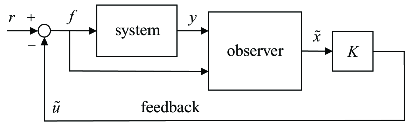
Figure 4: Block diagram of the state-feedback with observer.

The corresponding block diagram of a state-feedback control with observer is then shown in Fig. 4. Recall that for an asymptotically stable observation error $e(t)=x(t)-\tilde{x}(t)$, i.e. for

$$\underset{t\rightarrow\infty}{\lim}\|e(t)\|=0,$$

the system matrix of the observation error dynamics

$$\dot{e}(t)=\tilde{A}e(t)=(A-QC)e(t),$$

must be Hurwitz. For ensuring that the asymptotic observer operates efficiently in combination with a state-feedback control, the corresponding poles of $\tilde{A}$ are required generally to be significantly faster than those of $A^{*}$. Also recall that once the state-feedback, which includes observer, is closed, cf. Fig. 4, the state estimation dynamics becomes

$$\dot{\tilde{x}}=(A-BK-QC)\tilde{x}+Bf+Qy.$$ (11)

Despite the well-known separation principle of designing Luenberger observer, that allows the poles of both, observer and state-feedback, to be assigned independent of each other, a practical realization of the closed-loop as in Fig. 4 reveals less feasible for the system class introduced in section II-A. Next, we are to demonstrate it, while stressing that an observer-based state-feedback control as in Fig. 4 is well established and acknowledged (also in applications) for multiple other types of the observable systems.

III-B Practical infeasibility

While the designed observer and the state-feedback loop based on it have both a stable pole dynamics, we are to address additional stability features, that from a loop transfer function point of view, cf. Fig. 4. The observer-based open-loop transfer function from $r(s)$ to $\tilde{u}(s)$ is

$$L_{o}(s)=K\bigl{(}sI-A+BK+QC\bigr{)}^{-1}\,\bigl{[}B\,Q\bigr{]}\,\left[\begin{array}[]{c}1\\ G(s)\\ \end{array}\right],$$ (12)

with the identity matrix $I$ (of an appropriate dimension) and

$$G(s)=C(sI-A)^{-1}B.$$

Note that without use of observer (i.e. if the full state $x(t)$ is measurable), the open-loop transfer function is given by

$$L_{m}(s)=K\bigl{(}sI-A)^{-1}B.$$ (13)

Further we note that in both above cases, the open-loop transfer functions are not including the additional (disturbing) actuator dynamics $F(s)$, cf. (4). Thus, also the corresponding open loop transfer functions $F(s)L_{o}(s)$ and $F(s)L_{m}(s)$, respectively, will be inspected when analyzing the practical infeasibility. Now, let us make use of the so-called stability margin or maximum sensitivity (see e.g. [17] for details), which is defined as the maximum magnitude, i.e.

$$S_{\max}=\underset{\Omega}{\max}\,\bigl{|}S(i\Omega)\bigr{|}=\underset{\Omega}{\max}\,\Bigl{|}\bigl{(}1+L(i\Omega)\bigr{)}^{-1}\Bigr{|},$$ (14)

of the corresponding sensitivity function $S(\cdot)$ of any open-loop transfer function $L(\cdot)$. The latter is evaluated in frequency domain, where $\Omega$ in the angular frequency variable and $i$ is the imaginary unit satisfying $i^{2}=-1$. Recall that $S_{\max}$ indicates how close the Nyquist plot of the open-loop transfer function bypasses from the right the critical point $(-1,0)$ in the complex plane, cf. [17]. Thus, it represents a, to say, stability capacity of the closed-loop system and is typically required to be $S_{\max}<2\approx 6$ dB. Systems that have the loop transfer function with $S_{\max}>4\approx 12$ dB indicate a poor performance as well as poor robustness, cf. [18]. Further we note that for the closed-loop system with the structure as in Fig. 4, the sensitivity function represents the transfer characteristics between the reference value and the input to the system plant.

Now, consider a pole placement design of the above stated observer and the enclosing state-feedback control loop of the system (5). The exemplary assigned poles of the state feedback control are $\lambda_{c}=\{-40,-42,-44,-60\}$ and those of the asymptotic observer are $\lambda_{o}=\{-498,-503,-508,-513\}$. Note that all poles are real and placed sufficiently close to each other, for observer and controller respectively, thus providing an approximately same time-scale of the natural behavior of the all corresponding states. Here, the observer’s poles are approximately two and a half times faster than those of the closed-loop. All four sensitivity functions, with and without use of the observer, and also incorporating or not the actuator dynamics, are shown in Fig. 5.

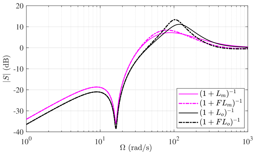
Figure 5: Sensitivity function of state-feedback control loop with and without the use of observer.

One can recognize that already the state-feedback without observer has a poor stability margin. When using observer, the $S_{\max}$ peak is further growing and becomes sharper and, in case of the actuator dynamics, reaches even 13.4 dB value. Recall here that a step reference will excite all frequencies, so that the input constraints (cf. section II-A) can then be violated during transients.

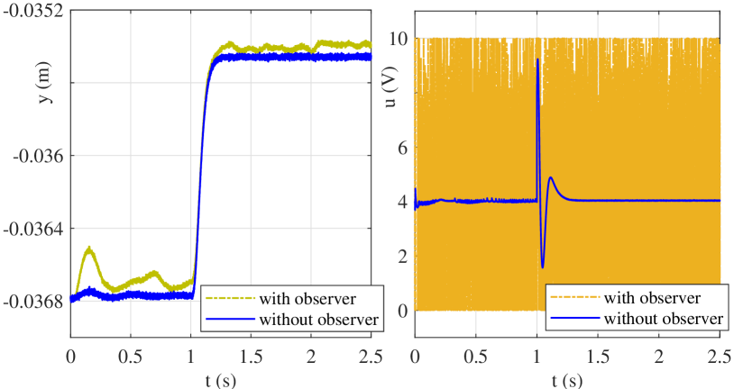
Figure 6: Simulated response with and without observer.

The implemented model (1)–(5) is used in a numerical simulation of the state-feedback control with and without observer designed as above. The simulated output $y(t)$ is subject to a minor (lower than in the experimental system) measurement noise. Also the step reference $r(t)$ is chosen so that the state-feedback control without observer is not saturated, cf. section II-B. The fixed-step solver with the sampling time 0.0002 sec (same as in the real-time experiments) is used. The output response and the control value of the simulation are shown for both cases in Fig. 6. One can see that in case of observer, the control value comes permanently in a high-frequent saturated behavior, that makes the observer-based control practically infeasible.

IV Time delay based control

IV-A Time delay based control

The time delay based feedback control of the fourth-order oscillatory systems, initially proposed in [4], is analyzed in detail in [5], also providing an experimental evaluation in combination with a standard PI (proportional-integral) controller. The time delay based control

$$u_{d}(t)=\alpha\bigl{(}y(t)-y(t-\theta)\bigr{)},$$ (15)

relies on the knowledge of the system parameter $\omega$, and assumes the time delay constant

$$\theta=-\arg\bigl{[}G(i\omega)\bigr{]}\omega^{-1},$$ (16)

and the gaining factor $\alpha>0$ which is the design parameter. The system transfer function in frequency domain is

$$G(i\Omega)=\frac{y(i\Omega)}{u(i\Omega)}=C\bigl{(}i\Omega I-A\bigr{)}^{-1}B.$$ (17)

Recall that the time delay based control (15) is largely attenuating the system resonance peak around $\omega_{0}$ without much reshaping the $G(i\Omega)$ transfer characteristics at other frequencies. Expressing the transfer function (17) as a ratio $G(i\Omega)=N(i\Omega)P(i\Omega)^{-1}$ of the corresponding polynomials $N(\cdot)$ and $P(\cdot)$, and rewriting (15) in frequency domain as

$$U_{d}(i\Omega)=\alpha\Bigl{(}1-\exp\bigl{(}-i\Omega\>\theta\bigr{)}\Bigr{)},$$ (18)

one can show that the closed-loop $G_{cl}=N(P-NU_{d})^{-1}$ is reshaping the system plant transfer characteristics as

$$R(i\Omega)=\frac{G(i\Omega)}{G_{cl}(i\Omega)}=1-\frac{N(i\Omega)U_{d}(i\Omega)}{P(i\Omega)}.$$ (19)

The reshaping (19) of the system transfer characteristics, here without constant disturbance $D$ and assuming in (4) $\tau=0$, is exemplary shown in Fig. 7 for $\alpha=100$.

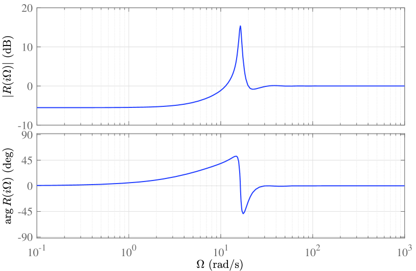
Figure 7: Reshaping (19) of system transfer characteristics.

One can recognize that the principal difference between the original system plant $G(i\Omega)$ and that one with the time delay based compensator, i.e. $G_{cl}(i\Omega)$, is precisely the resonance peak of $G(i\Omega)$. At higher frequencies, there is no changes in the amplitude response, while at lower frequencies an acceptable gain reduction is by approximately $-5$ dB. This can be then taken into account when the resonance-compensated system $G_{cl}(i\Omega)$ will be closed by an outer tracking control, cf. [5]. One can also recognize that the phase response of $G(i\Omega)$ and $G_{cl}(i\Omega)$ are essentially the same to left- and right-hand-side of the resonance frequency.

IV-B Robust frequency estimator

The robust frequency estimator, proposed in [12], can be used for online tuning of the $\omega$-parameter, provided the measured oscillatory signal $w(t)$ in unbiased. The estimator dynamics is given by, cf. [12],

$$\left(\begin{array}[]{c}\dot{\eta}_{1}\\ \dot{\eta}_{2}\\ \end{array}\right) = \left(\begin{array}[]{cc}0&1\\ -\tilde{\omega}^{2}&-2\tilde{\omega}\\ \end{array}\right)\left(\begin{array}[]{c}\eta_{1}\\ \eta_{2}\\ \end{array}\right)+\left(\begin{array}[]{c}0\\ 2\tilde{\omega}\\ \end{array}\right)w,$$ (28)

$$\nu = \left(\begin{array}[]{cc}0&1\\ \end{array}\right)\left(\begin{array}[]{c}\eta_{1}\\ \eta_{2}\\ \end{array}\right),$$ (32)

with the frequency-estimate adaptation law given by

$$\dot{\tilde{\omega}}=-\gamma\,\tilde{\omega}\,\mathrm{sign}(\eta_{1})(w-\nu).$$ (33)

Here $\gamma>0$ is the gain parameter of estimation. Note that the right-hand-side of (33) includes (in addition in comparison to [12]) a multiplication by $\tilde{\omega}$, so as to avoid the frequency estimate $\tilde{\omega}$ bypassing into the negative range. For details on the stability and performance of the robust frequency estimator the reader is referred to [12].

In order for a biased oscillation output $y(t)$ can equally be used in the frequency estimator (32), (33), the following dynamic bias-cancelation is proposed

$$w(t)=y(t)-y\Bigl{(}t-\frac{\pi}{\beta}\Bigr{)},\quad\omega<\beta<3\omega,$$ (34)

where $\beta$ is a free adjustable time-delay parameter. Assuming a biased (by $Y_{0}$) harmonic oscillation

$$y(t)=Y_{0}+Y\sin\bigl{(}\omega t+\phi\bigr{)},$$ (35)

and substituting it into (34) results in

$$w(t)=Y\biggl{(}\sin\bigl{(}\omega t+\phi\bigr{)}-\sin\Bigl{(}\omega t+\phi-\omega\frac{\pi}{\beta}\Bigr{)}\biggr{)}.$$ (36)

One can recognize that (36) constitutes also a harmonic signal with the same fundamental frequency $\omega$. The signal is unbiased and has another amplitude and phase comparing to the harmonic part of (35). Also worth noting is that $w(t)$ is not zero signal as long as $\omega\pi\beta^{-1}\neq 0$. If some nominal or upper-bound value of $\omega$ is known, the phase shifting factor $\beta$ can be assigned in a relatively large range, cf. (34).

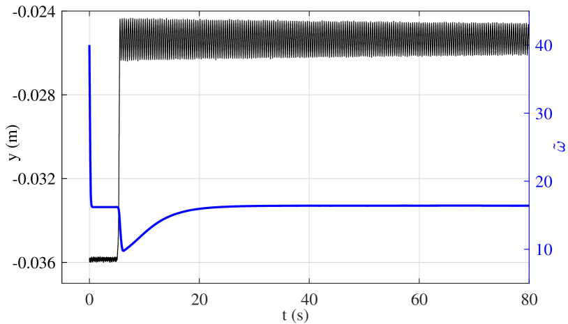
Figure 8: Converging $\tilde{\omega}(t)$ versus measured oscillating $y(t)$.

Since the robust estimator (32), (33) is unsensitive to both, the phase $\phi$ and slow variations of $Y$, see [12], the bias-freed input (36) can directly be used for estimation of $\tilde{\omega}$. Recall that $\tilde{\omega}(t)$ has a convergence behavior which rate is controllable by $\gamma$. An exemplary convergence of $\tilde{\omega}$ is shown in Fig. 8 together with the used $y(t)$ measurement. Note that the measured output is biased before and after the step-wise excitation. The initial value is set to $\tilde{\omega}(0)=40$ and the gain to $\gamma=200$. One can recognize that after the exciting transient of $y(t)$, the $\tilde{\omega}(t)$ is re-converging towards its final value $\approx 16.4$ rad/sec.

V Experimental control evaluation

A standard PI feedback controller

$$u_{pi}(t)=K_{p}e(t)+K_{i}\int e(t)dt,$$ (37)

operating on the output error $e(t)=r(t)-y(t)$, with $r(t)$ to be the set reference value for oscillatory load, can be desirable for the following reasons. (i) The single available system state is $y(t)$. (ii) An integral control action is required for guaranteeing a steady-state accuracy. (iii) An additional differential control action (i.e. resulting in PID control) is not contributing to stabilization of the oscillatory load in the fourth-order system (5). (iv) A state-feedback control, that requires an additional state observer, fails practically for the systems (2), (3), as discussed in detail in section III. At the same time, one can show that the open-loop transfer function $L(i\Omega)=y(s)/r(s)=PI(i\Omega)G(i\Omega)$, where $PI(i\Omega)$ is the transfer function corresponding to (37), has a marginal or even none gain margin. For basics on the gain margin and loop transfer function analysis we refer to e.g. [16]. Also the so-called maximum sensitivity (cf. e.g. [17]) will have a relatively high number for the corresponding $S(i\Omega)=\bigl{(}1+L(i\Omega)\bigr{)}^{-1}$, cf. with analysis made in section III. This indicates then a low stability for the closed-loop system.

The overall control law (evaluated experimentally) is

$$u(t)=u_{pi}(t)+u_{d}(t)+4.035,$$ (38)

where the last constant right-hand-side term compensates for the known gravity disturbance, cf. (2), (3), (4). Note that for the assigned $K_{p}=100$, $K_{i}=170$, cf. [5], the loop transfer function $L(\cdot)$ without (18) has a sufficient phase margin of 46 deg, but the missing gain margin of $-4.2$ dB.

First, the closed-loop response controlled with (38) is experimentally evaluated, as shown in Fig. 9, once without the time delay control part (i.e. with $\alpha=0$) and once with the time delay control part with $\alpha=100$. Note that here a fixed time delay constant, cf. section IV-A, is assigned from the known system parameter $\omega$.

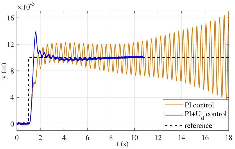
Figure 9: Controlled $y(t)$ by $PI$ control (i.e. $\alpha=0$) and $PI+U_{d}$ control with $\alpha=100$ and fixed $\theta$ value.

While the time delay based control provides a relatively fast cancelation of the otherwise oscillating output, cf. also with Fig. 3, the pure PI control drives the system to a visible instability over the time.

Next, the feedback control (38) is experimentally evaluated when applying an online adaptation of $\theta$ by means of the robust frequency estimator described in section IV-B. The adaptation gain is assigned to $\gamma=600$. The results are shown in Fig. 10, where the controlled output in depicted in (a), and the time progress of the $\tilde{\omega}(t)$ estimate is depicted in (b). Also the manual mechanical disturbances, which are additionally exciting the output oscillations, were applied, once by pushing down and once by pushing up the passive load, see in Fig. 10 (a) marked by the arrows.

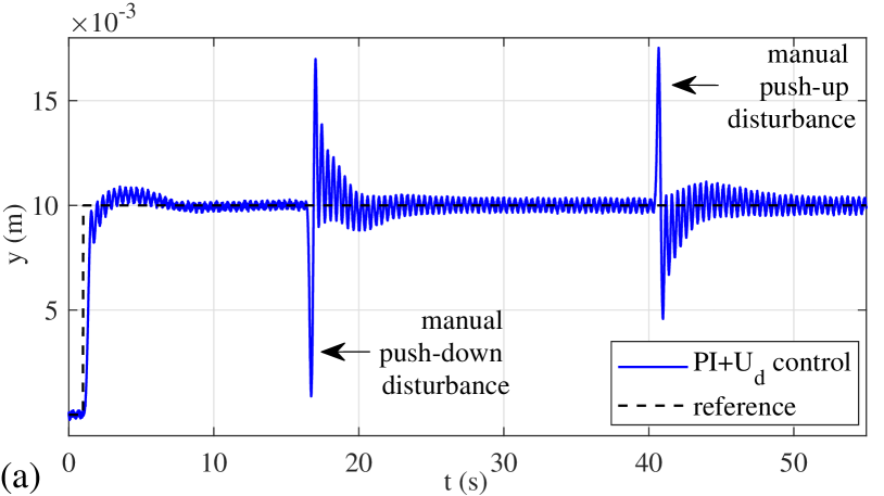
Figure 10: Controlled $y(t)$ with $PI+U_{d}$ and $\alpha=100$ and online adapted $\theta$ in (a), disturbance instants are marked; and convergence of $\tilde{\omega}(t)$ in (b).

One can recognize both, a stable attenuation of the output oscillations and a robust convergence of the $\tilde{\omega}(t)$ estimate. Important to notice is also that due to some (not modeled) nonlinear by-effects in the stiffness, the oscillation frequency $\omega$ experiences certain variations depending on the amplitude of $y(t)$, here elongation of the connecting spring.

For further evaluating robustness of the adaptive control (38), i.e. including online estimation of $\tilde{\omega}$, the experiments are performed for oscillatory initial conditions, see Fig. 11. The control parameters are the same as above. One can recognize a largely oscillating $y(t)$ before the step reference is applied.

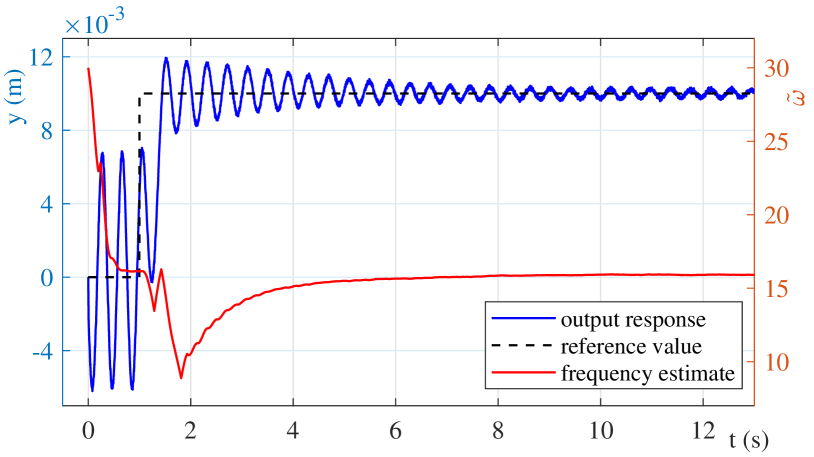
Figure 11: Controlled $y(t)$ with $PI+U_{d}$, $\alpha=100$ and the oscillatory initial conditions versus the convergence of $\tilde{\omega}(t)$ estimate.

For largely (i.e. more pronounced) oscillations of $y(t)$, the $\tilde{\omega}(t)$ estimate converges faster, which is then perturbed by the output transient with $Y_{0}\neq\mathrm{const}$, cf. (35). After the transient, the convergence of $\tilde{\omega}(t)$ recovers.

VI Conclusions

In this paper, we have discussed the fourth-order non-collocated systems with low-damped oscillating passive loads. Approaching the real applications, an actuator body is subject to the input and output constraints. We analyzed and demonstrated numerically that an observer-based state-feedback control reveals practically infeasible, despite the system dynamics proves to be observable. As a robust alternative, the time delay based control [4, 5] was applied for stabilizing the otherwise unstable PI controller of the set reference. The bias-canceling extension of the robust frequency estimator [12] was introduced, that allows for an online (adaptive) tuning of the time delay based controller. Various dedicated experiments were shown as confirmatory.

References

- [1] J. Vaughan, D. Kim, and W. Singhose, “Control of tower cranes with double-pendulum payload dynamics,” IEEE Transactions on Control Systems Technology, vol. 18, no. 6, pp. 1345–1358, 2010.
- [2] J. Wang and W. T. van Horssen, “On resonances and transverse and longitudinal oscillations in a hoisting system due to boundary excitations,” Nonlinear Dynamics, vol. 111, pp. 5079–5106, 2023.
- [3] B. Besselink, T. Vromen, N. Kremers, and N. Van De Wouw, “Analysis and control of stick-slip oscillations in drilling systems,” IEEE Transactions on Control Systems Technology, vol. 24, no. 5, pp. 1582–1593, 2015.
- [4] M. Ruderman, “Robust output feedback control of non-collocated low-damped oscillating load,” in IEEE 29th Mediterranean Conference on Control and Automation (MED), 2021, pp. 639–644.
- [5] M. Ruderman, “Time-delay based output feedback control of fourth-order oscillatory systems,” Mechatronics, vol. 94, p. 103015, 2023.
- [6] C.-Y. Kao and B. Lincoln, “Simple stability criteria for systems with time-varying delays,” Automatica, vol. 40, no. 8, pp. 1429–1434, 2004.
- [7] E. Fridman and U. Shaked, “Input–output approach to stability and l2-gain analysis of systems with time-varying delays,” Systems & Control Letters, vol. 55, no. 12, pp. 1041–1053, 2006.
- [8] K. Gu, V. Kharitonov, and J. Chen, Stability of time-delay systems. Springer, 2003.
- [9] W. Michiels and S.-I. Niculescu, Stability, control, and computation for time-delay systems: an eigenvalue-based approach. SIAM, 2014.
- [10] E. Fridman, “Tutorial on lyapunov-based methods for time-delay systems,” European Journal of Control, vol. 20, no. 6, pp. 271–283, 2014.
- [11] D. Liberzon, Switching in systems and control. Springer, 2003.
- [12] M. Ruderman, “One-parameter robust global frequency estimator for slowly varying amplitude and noisy oscillations,” Mechanical Systems and Signal Processing, vol. 170, p. 108756, 2022.
- [13] B. Voß, M. Ruderman, C. Weise, and J. Reger, “Comparison of fractional-order and integer-order H-infinity control of a non-collocated two-mass oscillator,” IFAC-PapersOnLine, vol. 55, pp. 145–150, 2022.
- [14] P. Antsaklis and A. Michel, A Linear Systems Primer. Birkhäuser Boston, 2007.
- [15] D. Luenberger, “An introduction to observers,” IEEE Transactions on Automatic Control, vol. 16, no. 6, pp. 596–602, 1971.
- [16] G. Franklin, J. Powell, and A. Emami-Naeini, Feedback control of dynamic systems. Pearson, 2020.
- [17] K. J. Åström and R. M. Murray, Feedback systems: an introduction for scientists and engineers. Princeton University Press, 2021.
- [18] S. Skogestad and I. Postlethwaite, Multivariable feedback control: analysis and design. John Wiley & Sons, 2005.