Distributed Consensus of Heterogeneous Multi-Agent Systems Based on Feedforward Control

Abstract

This paper studies the consensus problem of heterogeneous multi-agent systems by the feedforward control and linear quadratic (LQ) optimal control theory. Different from the existing consensus control algorithms, which require to design an additional distributed observer for estimating the leader’s information and to solve a set of regulator equations. In this paper, by designing a distributed feedforward controller, a non-standard neighbor error system is transformed into a standard linear system, and then an optimal consensus controller is designed by minimizing a combined state error with neighbour agents. The proposed optimal controller is obtained by solving Riccati equations, and it is shown that the corresponding cost function under the proposed distributed controllers is asymptotically optimal. The proposed consensus algorithm can be directly applicable to solve the consensus problem of homogeneous systems. Simulation example indicates the effectiveness of the proposed scheme and a much faster convergence speed than the existing algorithm.

I Introduction

In recent years, multi-agent systems has attracted considerable attentions for its extensive engineering applications in unmanned aerial vehicles and satellite formation, distributed robotics and wireless sensor networks [1, 2, 3]. Consensus problem of multi-agent system is an important and fundamental problem, whose essential task is to design a distributed controller based on the interaction with neighbor agents such that all agents achieve an agreement. A general framework of the consensus problem for first-order integrator networks is addressed with a fixed topology in [4]. [5] further proposes leader-following consensus algorithms for second-order integrator agents. [6] and [7] develop necessary and sufficient conditions for consensusability of discrete-time and continuous-time multi-agent systems, respectively. Variants of these algorithms have been designed with different communication topologies, system dynamics and performance requirements, see the works [8, 9, 10, 11] and the references therein. It is noted that the aforementioned works focus on homogeneous multi-agent systems with the identical dynamics for each agent.

However, in practice, many systems are heterogeneous with different system dynamics and even state space dimension. Under the circumstances, the traditional state consensus algorithm based on Kronecker product method is not applicable, so the consensus problem of heterogenous multi-agent system is more challenging than the homogeneous case. In recent years, the distributed feedforward control approach [12, 13] has been widely used in solving the consensus problem of heterogeneous multi-agent systems. Based on the feedforward control theory framework, researchers also further studied the robust output regulation problem [14], leader-follower consensus for uncertain nonlinear system subject to communication delays and switching networks [15], and bipartite output consensus over cooperative-competition networks [16], to name just a few. The core of this method includes two points: one significant point is the design of distributed observer or compensator to estimate the leader’s state; another necessary part is the solving of output regulation equations. It’s should be pointed that the chosen of the coupling gain to ensure the stability of distributed observer is dependent on the eigenvalues of the communication topology. Besides, in light with the distributed internal model method [17], some effort has also been done to the consensus of heterogeneous systems [18], while an internal model requirement is necessary and sufficient for synchronizability of heterogeneous agents, and a transmission zero condition never holds when the dimension of the system output is greater than that of the system input. Moreover, to our knowledge, the existing consensus algorithms for heterogeneous multi-agent systems may be hard directly reduced to that of the homogeneous case.

Inspired by the above analyses, in this paper, we study the consensus problem of heterogeneous multi-agent systems with a novel consensus control protocol based on the feedforward control and LQ optimal control theory. Compared with the existing results, the main contributions of this work are: 1) Since each agent is of different dynamics, we first design a distributed feedforward controller based on the state and input from neighbor agents, a non-standard error system with neighbour agents can be converted into a standard linear system. Then, an optimal feedback controller based on the observer incorporating each agent’s historical state information is designed by minimizing the state error of different neighbour agents; 2) The proposed feedback controller is obtained by solving Riccati equations, and the corresponding global cost function under the proposed controllers are asymptotically optimal; 3) No pre-design an additional distributed observer for the reference system, and remove the solvability assumption of output regulation equations, the proposed consensus control algorithm can be directly reduced to solve the consensus problem of the homogeneous systems, which is entirely different from the existing consensus algorithms.

The following notations will be used throughout this paper: $\mathbb{R}^{n\times m}$ represents the set of $n\times m$-dimensional real matrices. $I_{p}$ is the identity matrix with a dimension $p\times p$ $\mbox{diag}\{a_{1},a_{2},\cdots,a_{N}\}$ denotes the diagonal matrix with diagonal elements being $a_{1},\cdots,a_{N}$. $\|x\|$ is the 2-norm of a vector $x$. $\rho(A)$ is the spectral radius of matrix $A$. $A^{{\dagger}}$ and $A^{T}$ denote the transpose and the Moore-Penrose inverse of a matrix $A$. $Rang(A)$ denotes the range of $A$.

Let the interaction among $N+1$ agents be described by a directed graph $\mathcal{G}=\{\mathcal{V},\mathcal{E},\mathcal{A}\}$, where $\mathcal{V}=\{0,1,2,\cdots,N\}$ is the set of vertices (nodes), $\mathcal{E}\subseteq\mathcal{V}\times\mathcal{V}$ is the set of edges. Here, the node $0$ is associated with the leader system, and the node $i=1,\cdots,N$ is associated with the followers systems. $\mathcal{A}=[a_{ij}]\in\mathbb{R}^{(N+1)\times(N+1)}$ is the weight matrix of $\mathcal{G}$, $a_{ij}\neq 0$ if and only if the edge $(i,j)\in\mathcal{E}$, i.e., agent $j$ can use the state or the input of agent $i$ for control. The neighbor of agent $i$ is denoted by $\mathcal{N}_{i}=\{j|(i,j)\in\mathcal{E}\}$. A directed graph has a directed spanning tree if there exists a node called root such that there exists a directed path from this node to every other node.

II Problem Formulation

We consider a heterogeneous discrete-time multi-agent system consisting of $N$ agents over a directed graph $\mathcal{G}$ with the dynamics of each agent given by

$$x_{i}(k+1)=A_{i}x_{i}(k)+B_{i}u_{i}(k),i=1,2,\cdots,N$$ (1)

where $x_{i}(k)\in\mathbb{R}^{n}$ and $u_{i}(k)\in\mathbb{R}^{m_{i}}$ are the state and the input of each agent. $A_{i}\in\mathbb{R}^{n\times n}$ and $B_{i}\in\mathbb{R}^{n\times m_{i}}$ are the coefficient matrices, respectively.

The dynamic of the leader is given by

$$x_{0}(k+1)=A_{0}x_{0}(k),$$ (2)

where $x_{0}\in\mathbb{R}^{n\times n}$ is the state of the leader, and $A_{0}\in\mathbb{R}^{n\times n}$ is the system matrix.

The cost function of multi-agent systems (1) is given by

$$J(s,\infty) =\sum_{k=s}^{\infty}\left(\sum_{i=1}^{N}\sum_{j\in\mathcal{N}_{i}}(x_{i}(k)-x_{j}(k))^{T}Q(x_{i}(k)-x_{j}(k))\right.$$

$$\quad\left.+\sum_{i=1}^{N}u_{i}^{T}(k)R_{i}u_{i}(k)\right)$$ (3)

where $Q\geq 0$ and $R_{i}>0$ are weighting matrices.

We aim to design a distributed control protocol $u_{i}(k)$ based on the available information from neighbors for (1) to minimize the performance (II). In this case, heterogeneous multi-agent systems (1) and (2) can achieve the leader-follower consensus, i.e., for any initial conditions $x_{i0}$,

$$\lim_{k\to\infty}\|x_{i}(k)-x_{0}(k)\|=0,\quad i=1,\cdots,N.$$

Assumption 1.

The directed graph $\mathcal{G}$ has a spanning tree with the node $0$ as the root, i.e., $a_{i0}>0$.

III Main Results

III-A State consensus of heterogeneous multi-agent systems

Define the relative state error variables as:

$$e_{ij}(k)=x_{i}(k)-x_{j}(k),$$

then, the state error system is given by

$$e_{ij}(k+1) =A_{i}e_{ij}(k)+(A_{i}-A_{j})x_{j}(k)$$

$$\quad+B_{i}u_{i}(k)-B_{j}u_{j}(k)$$ (4)

with $i=1,\cdots,N$, $j\in\mathcal{N}_{i}$ and $B_{0}=0$.

Design the controllers as

$$u_{i}(k)=\tilde{u}_{i}(k)+\bar{u}_{i}(k),$$ (5)

where the feedforward control $\tilde{u}_{i}(k)$ is designed as:

$$\tilde{u}_{i}(k)=-B_{i}^{-1}(A_{i}-A_{j})x_{j}(k)+B_{i}^{-1}B_{j}u_{j}(k),$$ (6)

which only needs the state and input information from the neighbor agent $j$, so $\tilde{u}_{i}(k)$ in (6) is distributed. Under the feedforward control (6), the relative neighbor error system (III-A) is rewritten as the following standard linear system:

$$e_{ij}(k+1) =A_{i}e_{ij}(k)+B_{i}\bar{u}_{i}(k).$$ (7)

Then, the corresponding global error system is

$$E(k+1)=\tilde{A}E(k)+\tilde{B}\bar{u}(k),$$ (8)

where $E(k)=\begin{bmatrix}e_{10}^{T}(k)&\cdots&e_{ij}^{T}(k)\cdots&e_{N,N-1}^{T}(k)\end{bmatrix}^{T}$, $\bar{u}(k)=\begin{bmatrix}\bar{u}_{1}^{T}(k)&\bar{u}_{2}^{T}(k)\cdots&\bar{u}_{N}^{T}(k)\end{bmatrix}^{T}$, $\tilde{A}=diag\{A_{1},A_{2},\cdots,A_{N}\}$, and $\tilde{B}=diag\{B_{1},B_{2},\cdots,B_{N}\}$.

In this case, the cost function (II) is reformulated as

$$J(s,\infty) =\sum_{k=s}^{\infty}\left(\sum_{i=1}^{N}\sum_{j\in\mathcal{N}_{i}}e_{ij}^{T}(k)Qe_{ij}(k)+\sum_{i=1}^{N}\bar{u}_{i}^{T}(k)R_{i}\bar{u}_{i}(k)\right)$$

$$=\sum_{k=s}^{\infty}[E^{T}(k)\mathcal{Q}E(k)+\bar{u}^{T}(k)R\bar{u}(k)],$$ (9)

with $\mathcal{Q}=I_{N}\otimes Q$ and $R=diag\{R_{1},\cdots,R_{N}\}$.

Remark 1.

The designed distributed feedforward controller $\tilde{u}_{i}(k)$ in (6) needs the invertibility of the matrix $B_{i},i=1,\cdots,N$. When $B_{i}$ is irreversible, for any $x_{i}(k)\in\mathbb{R}^{n}$, the equation $B_{i}\tilde{u}_{i}(k)=(A_{i}-A_{j})x_{i}(k)$ has a solution if and only if $Rang(A_{i}-A_{j})\subseteq Rang(B_{i})$, then, for $\forall z(k)\in\mathbb{R}^{n}$, the feedforward controller is given by

$$\tilde{u}_{i}(k)=-B_{i}^{\dagger}(A_{i}-A_{j})x_{i}(k)+(I-B_{i}^{\dagger}B_{i})z(k).$$

Besides, when the system $(A_{i},B_{i})$ is uncontrollable, the solution for $\tilde{u}_{i}(k)$ can also be obtained by mismatch control method proposed in [19].

The following key task is to determine the feedback controller $\bar{u}_{i}(k)$ based on LQ optimal control theory. In the ideal (complete graph) case, the error information $E(k)$ is available for all agents, the solvability of the optimal control problem for system (8) with the cost function (III-A) is equivalent to the following standard LQ optimal control problem [20].

Lemma 1.

[20] Suppose that $E(k)$ is available for all agents, the optimal controller is given

$$\bar{u}^{*}(k)=KE(k)$$ (10)

where the feedback gain $K$ is given by

$$K=-(R+\tilde{B}^{T}P\tilde{B})^{-1}\tilde{B}^{T}P\tilde{A}$$ (11)

and $P$ is the solution of the following ARE

$$P=\tilde{A}^{T}P\tilde{A}+\mathcal{Q}-\tilde{A}^{T}P\tilde{B}(R+\tilde{B}^{T}P\tilde{B})^{-1}\tilde{B}^{T}P\tilde{A}.$$ (12)

The corresponding optimal cost function is

$$J^{*}(s,\infty)=E^{T}(s)PE(s).$$ (13)

Moreover, if $P$ is the unique positive definite solution to (12), then $\tilde{A}+\tilde{B}K$ is stable.

It’s obvious that multi-agent systems (1) and (2) can achieve leader-follower consensus under the centralized optimal controller (10). However, when $E(k)$ is not available for all agents, we next will design the decentralized controller based on observers incorporating agent’s historical state information.

To proceed further, the system (8) is rewritten as

$$E(k+1) =\tilde{A}E(k)+\sum_{i=1}^{N}\tilde{B}_{i}\bar{u}_{i}(k),$$ (14)

$$Y_{i}(k) =H_{i}E(k),i=1,\cdots,N$$ (15)

where $\tilde{B}_{i}=\begin{bmatrix}0&\cdots&B^{T}_{i}&0\cdots&0\end{bmatrix}^{T}$, $Y_{i}(k)$ is measurement, and $H_{i}$ is composed of $0$ and $I_{n}$, whose specific forms depend on the interaction among agents.

Next, we design a new distributed feedback controllers as

$$\bar{u}_{i}^{*}(k)=K_{i}\hat{E}_{i}(k)$$ (16)

where $\hat{E}_{i}(k)$ is a distributed observer based on the available information of agent $i$ to estimate the global error $E(k)$,

$$\hat{E}_{1}(k+1) =\tilde{A}\hat{E}_{1}(k)+\tilde{B}_{1}\bar{u}_{1}^{*}(k)+\tilde{B}_{2}K_{2}\hat{E}_{1}(k)+\cdots$$

$$\quad+\tilde{B}_{N}K_{N}\hat{E}_{1}(k)+L_{1}(Y_{1}(k)-H_{1}\hat{E}_{1}(k)),$$ (17a)

$$\quad\cdots\quad\cdots\quad\cdots$$

$$\hat{E}_{i}(k+1) =\tilde{A}\hat{E}_{i}(k)+\tilde{B}_{1}K_{1}\hat{E}_{i}(k)+\cdots$$

$$\quad+\tilde{B}_{i-1}K_{i-1}\hat{E}_{i}(k)+\tilde{B}_{i}\bar{u}_{i}^{*}(k)$$

$$\quad+\tilde{B}_{i+1}K_{i+1}\hat{E}_{i}(k)+\cdots+\tilde{B}_{N}K_{N}\hat{E}_{i}(k)$$

$$\quad+L_{i}(Y_{i}(k)-H_{i}\hat{E}_{i}(k))$$ (17b)

$$\quad\cdots\quad\cdots\quad\cdots$$

$$\hat{E}_{N}(k+1) =\tilde{A}\hat{E}_{N}(k)+\tilde{B}_{1}K_{1}\hat{E}_{N}(k)+\cdots$$

$$\quad+\tilde{B}_{N-1}K_{N-1}\hat{E}_{N}(k)+\tilde{B}_{N}\bar{u}_{N}^{*}(k)$$

$$\quad+L_{N}(Y_{N}(k)-H_{N}\hat{E}_{N}(k))$$ (17c)

where $K_{i}=\begin{bmatrix}0&\cdots&I&0\cdots&0\end{bmatrix}K$, which is obtained by solving ARE (12), $L_{i}$ is to be determined later to ensure the stability of the observers.

Theorem 1.

Assumption 1 holds. Consider the global error system (14), and the distributed control laws (16) with (17). If there exist observer gains $L_{i},i=1,\cdots,N$ such that the matrix

$$A_{c}=\begin{bmatrix}\Theta_{1}&-\tilde{B}_{2}K_{2}&\cdots&-\tilde{B}_{N}K_{N}\\ -\tilde{B}_{1}K_{1}&\Theta_{2}&\cdots&-\tilde{B}_{N}K_{N}\\ \vdots&\vdots&\ddots&\vdots\\ -\tilde{B}_{1}K_{1}&\cdots&-\tilde{B}_{N-1}K_{N-1}&\Theta_{N}\end{bmatrix}$$ (18)

is stable, where $\Theta_{i}=\tilde{A}+\tilde{B}K-\bar{B}_{i}K_{i}-L_{i}H_{i}$. Then the observers (17) are stable, i.e.,

$$\lim_{k\to\infty}\|\hat{E}_{i}(k)-E(k)\|=0.$$ (19)

Moreover, if the Riccati equation (12) has a positive definite solution $P$, under the distributed controllers (5) with (6) and (16), the multi-agent systems (1) and (2) can achieve leader-follower consensus.

Proof.

Define the observer error vector $\tilde{E}_{i}(k)=E(k)-\hat{E}_{i}(k)$. Then, combining system (14) with observers (17), one obtains

$$E(k+1) =(\tilde{A}+\tilde{B}K)E(k)-\tilde{B}_{1}K_{1}\tilde{E}_{1}(k)$$

$$-\tilde{B}_{2}K_{2}\tilde{E}_{2}(k)-\cdots-\tilde{B}_{N}K_{N}\tilde{E}_{N}(k)$$ (20)

$$\tilde{E}_{1}(k+1) =(\tilde{A}+\tilde{B}K-\tilde{B}_{1}K_{1}-L_{1}H_{1})\tilde{E}_{1}(k)$$

$$-\tilde{B}_{2}K_{2}\tilde{E}_{2}(k)-\cdots-\tilde{B}_{N}K_{N}\tilde{E}_{N}(k)$$ (21a)

$$\quad\cdots\quad\cdots\quad\cdots$$

$$\tilde{E}_{i}(k+1) =(\tilde{A}+\tilde{B}K-\tilde{B}_{i}K_{i}-L_{i}H_{i})\tilde{E}_{i}(k)$$

$$\quad-\tilde{B}_{1}K_{1}\tilde{E}_{1}(k)-\cdots-\tilde{B}_{i-1}K_{i-1}\tilde{E}_{i-1}(k)$$

$$\quad-\tilde{B}_{i+1}K_{i+1}\tilde{E}_{i+1}(k)-\cdots-\tilde{B}_{N}K_{N}\tilde{E}_{N}(k)$$ (21b)

$$\quad\cdots\quad\cdots\quad\cdots$$

$$\tilde{E}_{N}(k+1) =(\tilde{A}+\tilde{B}K-\tilde{B}_{N}K_{N}-L_{N}H_{N})\tilde{E}_{N}(k)$$

$$-\tilde{B}_{1}K_{1}\tilde{E}_{1}(k)-\cdots-\tilde{B}_{N-1}K_{N-1}\tilde{E}_{N-1}(k)$$ (21c)

According to (21), we have

$$\tilde{E}(k+1)=\tilde{A}_{c}\tilde{E}(k),$$ (22)

where $\tilde{E}(k)=\begin{bmatrix}\tilde{E}_{1}^{T}(k),\tilde{E}_{2}^{T}(k),\cdots,\tilde{E}_{N}^{T}(k)\end{bmatrix}^{T}$. Obviously, if there exist matrices $L_{i}$ such that $A_{c}$ is stable, then observer errors $\tilde{E}(k)$ converge to zero as $k\to\infty$, i.e., Eq. (19) holds. Furthermore, it follows from (III-A) and (21) that

$$\begin{bmatrix}E(k+1)\\ \tilde{E}(k+1)\end{bmatrix}=\bar{A}_{c}\begin{bmatrix}E(k)\\ \tilde{E}(k)\end{bmatrix}$$ (23)

where $\bar{A}_{c}=\begin{bmatrix}\tilde{A}+\tilde{B}K&\Psi\\ 0&A_{c}\end{bmatrix}$ and $\Psi=\begin{bmatrix}-\tilde{B}_{1}K_{1}&\cdots&-\tilde{B}_{N}K_{N}\end{bmatrix}$. Since $P$ is the positive definite solution to Riccati equation (12), then $\tilde{A}+\tilde{B}K$ is stable, based on the LQ control theory, the leader-follower consensus of multi-agent system (1) can be achieved, i.e., $\lim_{k\to\infty}\|x_{i}(k)-x_{0}(k)\|=0$ for $i=1,2,\cdots,N$.

The proof is completed.

∎

Observe from (23) that since $K$ has been given in (11), the consensus error system relies on $A_{c}$ which is determined by the observer gains $L_{i}$. Thus, to speed up the convergence of consensus, the remaining problem is to choose the matrix $L_{i},i=1,2,\cdots,N$ such that the spectral radius of $A_{c}$ is as small as possible. To this end, we can solve the following optimization problem: the minimization problem of the maximum singular value for $A_{c}$.

Lemma 2.

Let $\alpha>0$ such that

$$A_{c}^{T}A_{c}\leq\alpha I,$$

or

$$\begin{bmatrix}-\alpha I&A_{c}^{T}\\ A_{c}&-I\end{bmatrix}\leq 0,$$ (24)

where $A_{c}$ is as in (18). Then the optimal gain matrices $L_{i}$ are chosen by:

$$\min_{L_{i}}\alpha\quad\quad\mbox{s.t.}\quad\eqref{Lmi},\quad i=1,\cdots,N.$$ (25)

Remark 2.

Lemma 2 provides an approach to choose gain matrices $L_{i}$ such that the spectral radius of $A_{c}$ is as small as possible. But, sometimes this method may not guarantee the spectral radius of $A_{c}$ is less than $1$. In that case, we can determine $L_{i}$ by alternative linear matrix inequality methods.

Next, we will derive the cost difference between the proposed distributed controller (16), and the centralized optimal control (10), and then analyze the asymptotical optimal property of the corresponding cost function.

For the convenience of analysis, denote that

$$\mathcal{M}_{1} =(\tilde{A}+\tilde{B}K)^{T}P\Psi-\begin{bmatrix}K_{1}^{T}R_{1}K_{1}&\cdots&K_{N}^{T}R_{N}K_{N}\end{bmatrix},$$

$$\mathcal{M}_{2} =\begin{bmatrix}K_{1}^{T}R_{1}K_{1}&\cdots&0\\ 0&\ddots&0\\ \vdots&\vdots&\vdots\\ 0&\cdots&K_{N}^{T}R_{N}K_{N}\end{bmatrix}+\Psi^{T}P\Psi.$$

Theorem 2.

Under the proposed distributed controllers (16) and (17) with $L_{i},i=1,2,\cdots,N$ chosen from the optimization in Lemma 2, the corresponding cost function is given by

$$J^{\star}(s,\infty)$$

$$=E^{T}(s)PE(s)+\sum_{k=s}^{\infty}\begin{bmatrix}E(k)\\ \tilde{E}(k)\end{bmatrix}^{T}\begin{bmatrix}0&\mathcal{M}_{1}\\ \mathcal{M}_{1}^{T}&\mathcal{M}_{2}\end{bmatrix}\begin{bmatrix}E(k)\\ \tilde{E}(k)\end{bmatrix}$$ (26)

Moreover, the cost difference between the cost function (2) and the cost under the centralized optimal control is given by

$$\Delta J(s,\infty) =J^{\star}(s,\infty)-J^{*}(s,\infty)$$

$$=\sum_{k=s}^{\infty}\begin{bmatrix}E(k)\\ \tilde{E}(k)\end{bmatrix}^{T}\begin{bmatrix}0&\mathcal{M}_{1}\\ \mathcal{M}_{1}^{T}&\mathcal{M}_{2}\end{bmatrix}\begin{bmatrix}E(k)\\ \tilde{E}(k)\end{bmatrix}.$$ (27)

In particular, the optimal cost function difference will approach to zero as $s$ is sufficiently large. That is to say, the proposed consensus controller can achieve the optimal cost (asymptotically).

Proof.

According to (12) and (III-A), we have

$$E^{T}(k)PE(k)-E^{T}(k+1)PE(k+1)$$

$$=E^{T}(k)(\mathcal{Q}+K^{T}RK)E(k)$$

$$\quad-\tilde{E}^{T}(k)\Psi^{T}P(\tilde{A}+\tilde{B}K)E(k)$$

$$\quad-E^{T}(k)(\tilde{A}+\tilde{B}K)^{T}P\Psi\tilde{E}(k)-\tilde{E}^{T}(k)\Psi^{T}P\Psi\tilde{E}(k)$$

Based on the cost function (II) under the centralized optimal control, by performing summation on $k$ from $s$ to $\infty$ and applying algebraic calculations yields

$$E^{T}(s)PE(s)-E^{T}(\infty)PE(\infty)$$

$$=J(s,\infty)-\sum_{k=s}^{\infty}\begin{bmatrix}E(k)\\ \tilde{E}(k)\end{bmatrix}^{T}\begin{bmatrix}0&\mathcal{M}_{1}\\ \mathcal{M}_{1}^{T}&\mathcal{M}_{2}\end{bmatrix}\begin{bmatrix}E(k)\\ \tilde{E}(k)\end{bmatrix}$$ (28)

It follows from Theorem 1 that $\lim_{k\to\infty}E^{T}(k)PE(k)=0$. Therefore, the corresponding optimal cost function $J^{\star}(s,\infty)$ under the proposed distributed observer-based controller (16) is derived in (2). In line with (13), the optimal cost difference (2) holds. Furthermore, we can analyze the asymptotically optimality for the distributed controller (16), which is similar to that in [21]. To avoid repetition, it’s not described in this paper. This proof is completed. ∎

III-B Comparison with traditional consensus algorithms

Firstly, the consensus with the new controller has a faster convergence speed than the traditional consensus algorithms.

In fact, from the closed-loop system (23), one has

$$\left\|\begin{bmatrix}E(k)\\ \tilde{E}(k)\end{bmatrix}\right\|\leq\rho(\bar{A}_{c})\left\|\begin{bmatrix}E(k-1)\\ \tilde{E}(k-1)\end{bmatrix}\right\|,$$ (29)

where $\rho(\bar{A}_{c})$ is the spectra radius of $\tilde{A}+\tilde{B}K$ and $A_{c}$. In particularly, $\tilde{A}+\tilde{B}K$ is the closed-loop system matrix obtained by the optimal feedback control (11), that is, $E(k+1)=(\tilde{A}+\tilde{B}K)E(k)$ while $E(k+1)^{T}\mathcal{Q}E(k+1)$ is minimized as in (II), so the modulus of the eigenvalues for $\tilde{A}+\tilde{B}K$ is minimized in certain sense. Besides, based on the optimization in Lemma 2, we can appropriately select $L_{i}$ such that the upper bound of the spectral radius $\rho(A_{c})$ is as small as possible. From these perspectives, $\rho(\bar{A}_{c})$ is made more to be small. This is in comparison with the conventional consensus algorithms where the maximum eigenvalue of the matrix $\bar{A}_{c}$ is not minimized and determined by the eigenvalues of the Laplacian matrix $\mathcal{L}$. Therefore, it can be expected that the proposed approach can achieve a faster convergence than the conventional algorithms as demonstrated in the simulation examples in Section IV.

Second, the cost difference $\Delta J(s,\infty)$ between the new distributed controller (16) and the centralized optimal control (10) is provided in Theorem 2, and it is equal to zero as $s\to\infty$. That is to say, the corresponding cost function under the proposed distributed controllers (16) is asymptotically optimal.

Remark 3.

The proposed distributed consensus algorithms (5) with (6),(16) and (17) can be directly reduced to the homogeneous case [21], which is totally different from the relevant research works [13, 22, 17]. In the current works, the solvability assumption of output regulation equations and an additional distributed observer to estimate the leader’s state have been removed A kind of novel distributed controller based on the distributed feedforward control and observer containing decentralized information is developed to solve the output consensus problem of heterogeneous systems (1) and (2). Moreover, the feedback gain matrices $K_{i}$ are obtained by solving Riccati equations, which never require the calculation of eigenvalues for communication topology.

III-C Output consensus of heterogeneous multi-agent systems

Different from the cases discussed in Section III-A, where the state dimension of each subsystem is identical, we further study the output consensus of heterogeneous systems with different state space dimensions.

Consider the heterogeneous multi-agent systems consisting of $N$ followers, whose dynamics are given by

$$x_{i}(k+1) =A_{i}x_{i}(k)+B_{i}u_{i}(k),$$

$$y_{i}(k) =C_{i}x_{i}(k),i=1,2,\cdots,N$$ (30)

where $x_{i}(k)\in\mathbb{R}^{n_{i}}$ and $u_{i}(k)\in\mathbb{R}^{m_{i}}$ are the state and the input of each agent. $A_{i}\in\mathbb{R}^{n_{i}\times n_{i}}$ ,$B_{i}\in\mathbb{R}^{n_{i}\times m_{i}}$ and $C_{i}\in\mathbb{R}^{q\times n_{i}}$ are the coefficient matrices, respectively.

The dynamic of the leader is given by

$$x_{0}(k+1) =A_{0}x_{0}(k),$$

$$y_{0}(k) =C_{0}x_{0}(k)$$ (31)

where $x_{0}\in\mathbb{R}^{p\times p}$ and $y_{0}(k)\in\mathbb{R}^{q}$ is the state of the leader, $A_{0}\in\mathbb{R}^{p\times p}$ and $C_{0}\in\mathbb{R}^{q\times p}$ are the coefficient matrices.

The cost function of multi-agent systems (III-C) is given by

$$J(s,\infty) =\sum_{k=s}^{\infty}\left(\sum_{i=1}^{N}\sum_{j\in\mathcal{N}_{i}}(y_{i}(k)-y_{j}(k))^{T}Q(y_{i}(k)-y_{j}(k))\right.$$

$$\quad\left.+\sum_{i=1}^{N}u_{i}^{T}(k)R_{i}u_{i}(k)\right)$$ (32)

where $Q\geq 0$ and $R_{i}>0$ are weighting matrices.

Because the state space dimension of each subsystem is not identical, the above state consensus is meaningless. We need to design a distribute controller $u_{i}(k)$ to ensure the output of the followers synchronize to the leader’s output,i.e.,

$$\lim_{k\to\infty}\|y_{i}(k)-y_{0}(k)\|=0,\quad i=1,2,\cdots,N.$$

To this end, we define relative output error variables:

$$\varepsilon_{ij}(k)=y_{i}(k)-y_{j}(k),\quad j\in\mathcal{N}_{i}.$$ (33)

Then,

$$\varepsilon_{ij}(k+1) =\varepsilon_{ij}(k)+C_{i}(A_{i}-I_{n_{i}})x_{i}(k)+C_{i}B_{i}u_{i}(k)$$

$$\quad-C_{j}(A_{j}-I_{n_{j}})x_{j}(k)-C_{j}B_{j}u_{j}(k)$$ (34)

with $B_{0}=0,u_{0}(k)=0$ and $j\in\mathcal{N}_{i}$.

Similarly, we design the controllers $u_{i}(k)$ as

$$u_{i}(k)=\tilde{u}_{i}(k)+\bar{u}_{i}(k),$$ (35)

where the feedforward controller $\tilde{u}_{i}(k)$ is:

$$\tilde{u}_{i}(k) =-B_{i}^{-1}(A_{i}-I_{n_{i}})x_{i}(k)+(C_{i}B_{i})^{-1}(C_{j}B_{j})u_{j}(k)$$

$$\quad+(C_{i}B_{i})^{-1}C_{j}(A_{j}-I_{n_{j}})x_{j}(k).$$ (36)

Obvious the distributed feedforward controller $\tilde{u}_{i}(k)$ is designed by using only the state information of itself and its neighbor agent $j$ and the control input of neighbor agent $j$. Under the feedforward controller (III-C), the output error system (III-C) is converted into a standard linear system

$$\varepsilon_{ij}(k+1)=\varepsilon_{ij}(k)+C_{i}B_{i}\bar{u}_{i}(k),$$ (37)

the corresponding global form is

$$\Upsilon(k+1)=\mathcal{A}\Upsilon(k)+\mathcal{B}\bar{u}(k),$$ (38)

where $\Upsilon(k)=\begin{bmatrix}\varepsilon_{10}^{T}(k)&\cdots&\varepsilon_{ij}^{T}(k)\cdots&\varepsilon_{N,N-1}^{T}(k)\end{bmatrix}^{T}$, $\bar{u}(k)=\begin{bmatrix}\bar{u}_{1}^{T}(k)&\bar{u}_{2}^{T}(k)\cdots&\bar{u}_{N}^{T}(k)\end{bmatrix}^{T}$, $\mathcal{A}=I_{N}\otimes I_{q}$, and $\mathcal{B}=diag\{C_{1}B_{1},C_{2}B_{2},\cdots,C_{N}B_{N}\}$.

Then, the cost function (III-C) is reformulated as

$$J(s,\infty) =\sum_{k=s}^{\infty}\left(\sum_{i=1}^{N}\sum_{j\in\mathcal{N}_{i}}\varepsilon_{ij}^{T}(k)Q\varepsilon_{ij}(k)+\sum_{i=1}^{N}\bar{u}_{i}^{T}(k)R_{i}\bar{u}_{i}(k)\right)$$

$$=\sum_{k=s}^{\infty}[\Upsilon^{T}(k)\mathcal{Q}\Upsilon(k)+\bar{u}^{T}(k)R\bar{u}(k)],$$ (39)

with $\mathcal{Q}=I_{N}\otimes Q$ and $R=diag\{R_{1},\cdots,R_{N}\}$.

Next, we will focus on designing the feedback control $\bar{u}_{i}(k)$ by minimizing the performance (III-C).

We rewrite the system (38) as

$$\Upsilon(k+1) =\mathcal{A}\Upsilon(k)+\sum_{i=1}^{N}\mathcal{B}_{i}\bar{u}_{i}(k),$$ (40)

$$\mathcal{Y}_{i}(k) =F_{i}\Upsilon(k),i=1,\cdots,N$$ (41)

where $\mathcal{B}_{i}=\begin{bmatrix}0&\cdots&(C_{i}B_{i})^{T}&0\cdots&0\end{bmatrix}^{T}$, $\mathcal{Y}_{i}(k)$ is measurement, and $F_{i}$ is composed of $0$ and $I_{n}$, whose specific forms depend on the interaction among agents.

Next, we design a new distributed feedback controllers as

$$\bar{u}_{i}^{*}(k)=\mathcal{K}_{i}\hat{\Upsilon}_{i}(k)$$ (42)

where $\hat{\Upsilon}_{i}(k)$ is a distributed observer based on the available information of agent $i$ to estimate the global error $\Upsilon(k)$,

$$\hat{\Upsilon}_{1}(k+1) =\mathcal{A}\hat{\Upsilon}_{1}(k)+\mathcal{B}_{1}\bar{u}_{1}^{*}(k)+\mathcal{B}_{2}\mathcal{K}_{2}\hat{\Upsilon}_{1}(k)+\cdots$$

$$\quad+\mathcal{B}_{N}\mathcal{K}_{N}\hat{\Upsilon}_{1}(k)+\Phi_{1}(\mathcal{Y}_{1}(k)-F_{1}\hat{\Upsilon}_{1}(k)),$$ (43a)

$$\quad\cdots\quad\cdots\quad\cdots$$

$$\hat{\Upsilon}_{i}(k+1) =\mathcal{A}\hat{\Upsilon}_{i}(k)+\mathcal{B}_{1}\mathcal{K}_{1}\hat{\Upsilon}_{i}(k)+\cdots$$

$$\quad+\mathcal{B}_{i-1}\mathcal{K}_{i-1}\hat{\Upsilon}_{i}(k)+\mathcal{B}_{i}\bar{u}_{i}^{*}(k)$$

$$\quad+\mathcal{B}_{i+1}\mathcal{K}_{i+1}\hat{\Upsilon}_{i}(k)+\cdots+\mathcal{B}_{N}\mathcal{K}_{N}\hat{\Upsilon}_{i}(k)$$

$$\quad+\Phi_{i}(\mathcal{Y}_{i}(k)-F_{i}\hat{\Upsilon}_{i}(k))$$ (43b)

$$\quad\cdots\quad\cdots\quad\cdots$$

$$\hat{\Upsilon}_{N}(k+1) =\mathcal{A}\hat{\Upsilon}_{N}(k)+\mathcal{B}_{1}\mathcal{K}_{1}\hat{\Upsilon}_{N}(k)+\cdots$$

$$\quad+\mathcal{B}_{N-1}\mathcal{K}_{N-1}\hat{\Upsilon}_{N}(k)+\mathcal{B}_{N}\bar{u}_{N}^{*}(k)$$

$$\quad+\Phi_{N}(\mathcal{Y}_{N}(k)-F_{N}\hat{\Upsilon}_{N}(k))$$ (43c)

where $\mathcal{K}_{i}=\begin{bmatrix}0&\cdots&I&0\cdots&0\end{bmatrix}\mathcal{K}$, which is obtained by solving a ARE

$$\mathcal{P}=\mathcal{A}^{T}\mathcal{P}\mathcal{A}+\mathcal{Q}-\mathcal{A}^{T}P\mathcal{B}(R+\mathcal{B}^{T}\mathcal{P}\mathcal{B})^{-1}\mathcal{B}^{T}\mathcal{P}\mathcal{A}$$ (44)

and $\Phi_{i}$ is observer gain matrix to be determined later.

Theorem 3.

Under the distributed control laws (42) with (43), consider the global error system (40), If there exist observer gains $\Phi_{i},i=1,\cdots,N$ such that the matrix

$$H_{c}=\begin{bmatrix}\Sigma_{1}&-\mathcal{B}_{2}\mathcal{K}_{2}&\cdots&-\mathcal{B}_{N}\mathcal{K}_{N}\\ -\mathcal{B}_{1}\mathcal{K}_{1}&\Sigma_{2}&\cdots&-\mathcal{B}_{N}\mathcal{K}_{N}\\ \vdots&\vdots&\ddots&\vdots\\ -\mathcal{B}_{1}\mathcal{K}_{1}&\cdots&-\mathcal{B}_{N-1}\mathcal{K}_{N-1}&\Sigma_{N}\end{bmatrix}$$ (45)

is stable, where $\Sigma_{i}=\mathcal{A}+\mathcal{B}\mathcal{K}-\mathcal{B}_{i}\mathcal{K}_{i}-\Phi_{i}F_{i}$. Then the observers (43) are stable under the controller (42), i.e.,

$$\lim_{k\to\infty}\|\hat{\Upsilon}_{i}(k)-\Upsilon(k)\|=0.$$ (46)

Moreover, if the Riccati equation (44) has a positive definite solution $\mathcal{P}$, under the distributed controllers (III-C) and (42) with (43), the heterogeneous multi-agent systems (III-C) and (III-C) can achieve output consensus. The corresponding cost function is asymptotically optimal.

Proof.

This proof is similar to that in Theorem 1 and Theorem 2. So the details are omitted. ∎

IV Numerical Simulation

In this section, we validate the the proposed theoretical results through the following numerical example.

Example 1.

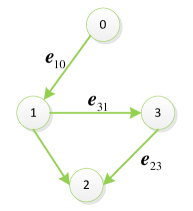
Figure 1: Communication topology among four agents

Consider the multi-agent system consisting of three heterogeneous follower agents with the system matrices:

$$A_{1} =\begin{bmatrix}1.1&1\\ -2&1\end{bmatrix},A_{2}=\begin{bmatrix}-2&1\\ 1&-1\end{bmatrix},A_{3}=\begin{bmatrix}0.5&0\\ -2&-0.6\end{bmatrix}$$

$$B_{1} =\begin{bmatrix}0&1\\ 0.4&0.2\end{bmatrix},B_{2}=\begin{bmatrix}0.1&0.2\\ 1&0.5\end{bmatrix},B_{3}=\begin{bmatrix}0.2&0\\ 0.1&1\end{bmatrix}$$

The leader’s state trajectory is generated by a sinusoidal trajectory generator, its dynamics is given by:

$$A_{0}=\begin{bmatrix}cos(0.5)&sin(0.5)\\ -sin(0.5)&cos(0.5)\end{bmatrix}.$$

The interactions of agents are given in Fig.1, which satisfies Assumption 1. Each agent only receives neighbor error information, so we can determine $H_{i}$ as

$$H_{1}=\begin{bmatrix}I_{2}&0&0\end{bmatrix},H_{2}=\begin{bmatrix}0&I_{2}&0\end{bmatrix},H_{3}=\begin{bmatrix}0&0&I_{2}\end{bmatrix}$$

We choose

$$Q=R_{1}=R_{2}=R_{3}=I_{2}.$$

According to ARE (12) and the Lemma (2), the feedback gains $K_{i}$ and the observer gain $L_{i}$ can be obtained, respectively. Fig.2 displays that the observer error vectors $\tilde{E}_{i}(k)$ under the proposed controller (16) converge to zero. The state trajectories of three followers and the leader are shown in Fig.4, which implies that the state of followers can synchronize with the state generated by the leader after 16 steps. With the same initial conditions, applying the existing consensus algorithm in [13], Fig.5 and Fig.6 show the first state trajectories for four agents and the state error trajectories between agents and the leader, respectively, To further compare the consensus speed with the traditional method, we calculate the spectral radius as $\rho(A_{c})=0.7860$ by our method, and according to the existing method, the spectral radius is $\rho(A_{c})=0.9651$. Therefore, Therefore, the proposed distributed controller (5) with (6),(16) and (17) can make all agents tack to the leader with a faster convergence speed.

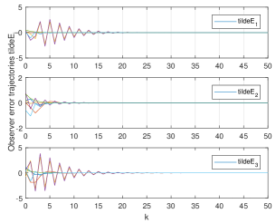
Figure 2: Observer error trajectories $\tilde{E}_{i}(k)$.

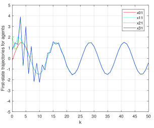
Figure 3: The first state trajectories of each agent $x_{i}(k),i=0,1,2,3$.

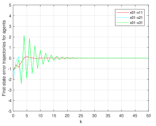
Figure 4: The first state error trajectories by the proposed method.

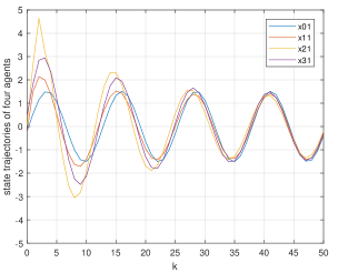
Figure 5: The first state trajectories of each agent by the existing method.

Figure 6: The first state error trajectories by the existing method.

V Conclusions

In this paper, we have studied the consensus problem for heterogeneous multi-agent systems by a new feedforward control approach and optimal control theory. The proposed new distributed controller has contained two parts: a distributed feedforward controller has been designed based on the information of agents and its neighbors, and then an optimal consensus controller based on observers involving agent’s historical state information has been obtained by solving Riccati equations. Different from the existing consensus control algorithms, the current algorithm has removed the requirements for designing an additional distributed observer and for solving a set of regulator equations. It is shown that the corresponding cost function under the proposed distributed controllers was asymptotically optimal. The proposed consensus algorithm can be directly reduced to the homogeneous systems. Simulation example indicated the effectiveness of the proposed scheme, the proposed approach can achieve a faster convergence than the conventional algorithms.

References

- [1] E. M. A. Wei Ren, Randal W. Beard, “Information consensus in multivehicle cooperative control,” IEEE Control Systems, vol. 27, no. 2, pp. 71–82, apr 2007.
- [2] R. Olfati-Saber, J. A. Fax, and R. M. Murray, “Consensus and cooperation in networked multi-agent systems,” Proceedings of the IEEE, vol. 95, no. 1, pp. 215–233, jan 2007.
- [3] Y. Yang, Y. Xiao, and T. Li, “Attacks on formation control for multiagent systems,” IEEE Transactions on Cybernetics, vol. 52, no. 12, pp. 12 805–12 817, dec 2022.
- [4] R. Olfati-Saber and R. Murray, “Consensus problems in networks of agents with switching topology and time-delays,” IEEE Transactions on Automatic Control, vol. 49, no. 9, pp. 1520–1533, sep 2004.
- [5] W. Ren and E. Atkins, “Distributed multi-vehicle coordinated controlvia local information exchange,” International Journal of Robust and Nonlinear Control, vol. 17, no. 10-11, pp. 1002–1033, 2007.
- [6] C.-Q. Ma and J.-F. Zhang, “Necessary and sufficient conditions for consensusability of linear multi-agent systems,” IEEE Transactions on Automatic Control, vol. 55, no. 5, pp. 1263–1268, may 2010.
- [7] K. You and L. Xie, “Network topology and communication data rate for consensusability of discrete-time multi-agent systems,” IEEE Transactions on Automatic Control, vol. 56, no. 10, pp. 2262–2275, oct 2011.
- [8] J. Huang, “The consensus for discrete-time linear multi-agent systems under directed switching networks,” IEEE Transactions on Automatic Control, vol. 62, no. 8, pp. 4086–4092, aug 2017.
- [9] Y. Zhu, S. Li, J. Ma, and Y. Zheng, “Bipartite consensus in networks of agents with antagonistic interactions and quantization,” IEEE Transactions on Circuits and Systems II: Express Briefs, vol. 65, no. 12, pp. 2012–2016, dec 2018.
- [10] J. Xu, Z. Zhang, and W. Wang, “Mean-square consentability of multiagent systems with nonidential channel fading,” IEEE Transactions on Automatic Control, vol. 66, no. 4, pp. 1887–1894, apr 2021.
- [11] F. Chen and J. Chen, “Minimum-energy distributed consensus control of multiagent systems: A network approximation approach,” IEEE Transactions on Automatic Control, vol. 65, no. 3, pp. 1144–1159, mar 2020.
- [12] Y. Su and J. Huang, “Cooperative output regulation of linear multi-agent systems,” IEEE Transactions on Automatic Control, vol. 57, no. 4, pp. 1062–1066, apr 2012.
- [13] J. Huang, “The cooperative output regulation problem of discrete-time linear multi-agent systems by the adaptive distributed observer,” IEEE Transactions on Automatic Control, vol. 62, no. 4, pp. 1979–1984, apr 2017.
- [14] C. Bi, X. Xu, L. Liu, and G. Feng, “Robust cooperative output regulation of heterogeneous uncertain linear multiagent systems with unbounded distributed transmission delays,” IEEE Transactions on Automatic Control, vol. 67, no. 3, pp. 1371–1383, 2022.
- [15] M. Lu and L. Liu, “Leader-following consensus of multiple uncertain euler–lagrange systems subject to communication delays and switching networks,” IEEE Transactions on Automatic Control, vol. 63, no. 8, pp. 2604–2611, aug 2018.
- [16] F. A. Yaghmaie, R. Su, F. L. Lewis, and S. Olaru, “Bipartite and cooperative output synchronizations of linear heterogeneous agents: A unified framework,” Automatica, vol. 80, pp. 172–176, jun 2017.
- [17] P. Wieland, R. Sepulchre, and F. Allgöwer, “An internal model principle is necessary and sufficient for linear output synchronization,” Automatica, vol. 47, pp. 1068–1074, 2011.
- [18] S. Zuo, Y. Song, F. L. Lewis, and A. Davoudi, “Output containment control of linear heterogeneous multi-agent systems using internal model principle,” IEEE Transactions on Cybernetics, vol. 47, no. 8, pp. 2099–2109, aug 2017.
- [19] S. Lv, H. Li, K. Peng, and H. Zhang, “An approach to mismatched disturbance rejection control for uncontrollable systems.” [Online]. Available: https://doi.org/10.48550/arXiv.2209.07014
- [20] J. M. B.D.O. Anderson, Linear optimal control. Prentice Hall, 1971.
- [21] L. Zhang, J. Xu, H. Zhang, and L. Xie, “Distributed optimal control and application to consensus of multi-agent systems,” 2023. [Online]. Available: https://doi.org/10.48550/arXiv.2309.12577
- [22] J. Zhang, T. Feng, X. Wang, S. Qiao, and F. Yan, “Output consensus for heterogeneous multi-agent systems with disturbances,” Journal of the Franklin Institute, vol. 357, no. 4, pp. 2457–2470, mar 2020.