Resfusion: Prior Residual Noise embedded Denoising Diffusion Probabilistic Models

Abstract

Recently, Denoising Diffusion Probabilistic Models have been widely used in image segmentation, by generating segmentation masks conditioned on the input image. However, previous works can not seamlessly integrate existing end-to-end models with denoising diffusion models. Existing research can only select acceleration steps based on experience rather than calculating them specifically. Moreover, most methods are limited to small models and small-scale datasets, unable to generalize to general datasets and a wider range of tasks. Therefore, we propose Resfusion with a novel resnoise-diffusion process, which gradually generates segmentation masks or any type of target image, seamlessly integrating state-of-the-art end-to-end models and denoising diffusion models. Resfusion bridges the discrepancy between the likelihood output and the ground truth output through a Markov process. Through the novel smooth equivalence transformation in resnoise-diffusion process, we determine the optimal acceleration step. Experimental results demonstrate that Resfusion combines the capabilities of existing end-to-end models and denoising diffusion models, further enhancing performance and achieving outstanding results. Moreover, Resfusion is not limited to segmentation tasks, it can easily generalize to any general tasks of image generation and exhibit strong competitiveness.

1 Introduction

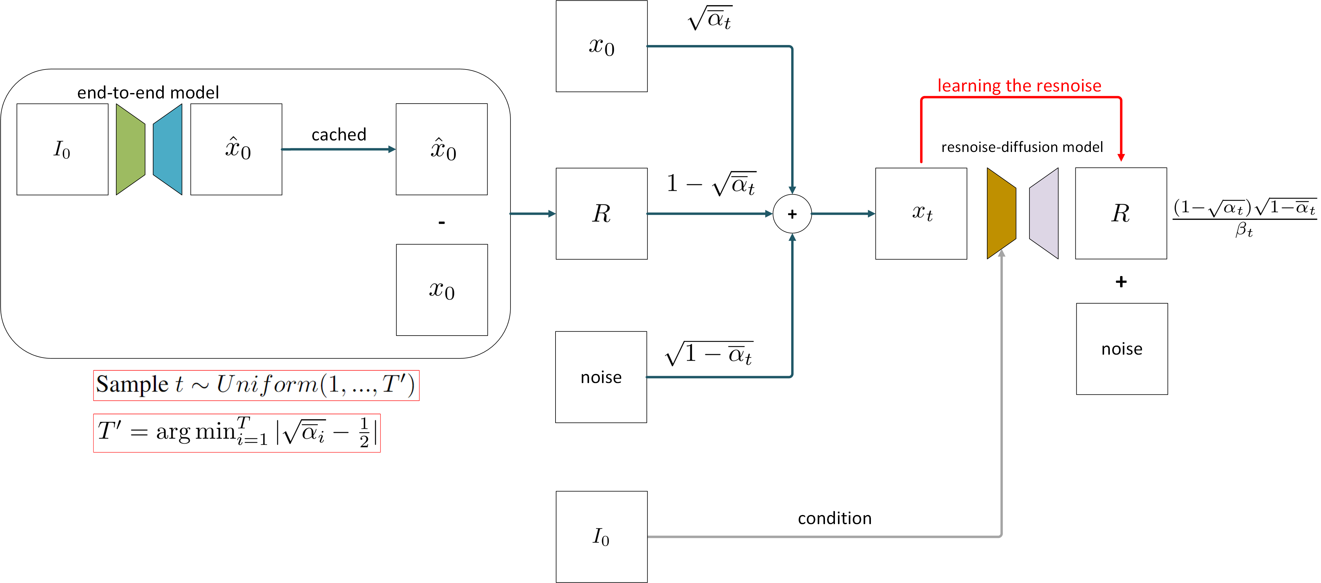
Figure 1: The training pipeline of Resfusion . $I_{0}$ represents the input image, which goes through an $E2EModel$ to obtain the likelihood output $\hat{x}_{0}$. $\hat{x}_{0}$ can be cached to avoid additional training cost. $R$ is the residual term defined through 18. ${x}_{t}$ is calaulated through 20. ${x}_{t}$, $t$, and conditioning input $I_{0}$ are fed into the resnoise-diffusion model to learn the resnoise.

Image segmentation seeks to categorize the pixels in an image into distinct classes. These classes can be delineated by various criteria, such as semantic categories or individual instances. Consequently, a range of image segmentation tasks has emerged, encompassing semantic segmentation[32], instance segmentation[19], and panoptic segmentation[26]. In recent years, researchers have introduced task-specific architectural approaches for a variety of image segmentation tasks[19, 8, 52, 56, 51].

Denoising Diffusion Probabilistic Models, originally introduced by Sohl-Dickstein et al. [42], Ho et al. [21], and Ho and Salimans [20], are generative models that generate data samples through an iterative denoising process. These models have demonstrated outstanding performance when compared to generative adversarial networks[16] and have served as the foundational framework for various image generation applications, including DALL·E 2[39], stable diffusion and Midjourney[40]. Due to the remarkable feature extraction capabilities of denoising diffusion models, some researchers have finetuned diffusion models and utilized their encoding and decoding capabilities for segmentation tasks[5, 41, 36]. Additionally, other works have employed cross-attention maps of intermediate features from diffusion models as additional conditions for segmentation tasks[58, 47, 50].

Amit et al. [2] first introduce the step-wise denoising process of diffusion denoising models into image segmentation. Formally, the diffusion-based segmentation model, conditioned on the original image, operates from random noise to gradually denoise and ultimately produces the corresponding segmentation mask. A series of studies emerged to modify and refine this process, encompassing the design of architecture[38, 3, 54, 62], improvements in the training procedure[14, 9, 13], enhancements to the denoising modules[49, 59, 55, 7, 57, 12], acceleration of the inference process[18, 17], and application to downstream tasks[35, 1, 24, 4, 23].

However, these methods have some limitations. First, there is no method that can seamlessly combine the existing end-to-end methods with the denoising diffusion models. Guo et al. [18, 17] proposed a pre-segmentation network to combine existing segmentation networks with the diffusion denoising models. However, they mainly focus on accelerating the reverse diffusion inference process, overlooking the asymmetry in the training process. Second, their training processes can not be accelerated, and their inference processes can not be accelerated without bias and can only select acceleration steps based on experience rather than calculating them specifically. Third, existing methods mainly concentrate on small models and small datasets in the medical field, which restricts the generalization performance of the model.

In this work, We propose the Resfusion , a framework that gradually generates target images in a coarse-to-fine manner, seamlessly integrating current state-of-the-art end-to-end models and denoising diffusion models. Our contributions can be summarized as follows:

• First, we propose a novel resnoise-diffusion process to close the gap between the likelihood output and ground truth output through a Markov process. By learning the resnoise between the likelihood output and ground truth output, We unified the training and inference denoising processes through resnoise-diffusion, seamlessly integrates the end-to-end and denoising diffusion models.

• Second, through the novel smooth equivalence transformation in resnoise-diffusion process, we determine the optimal acceleration step $T^{\prime}$. When the total steps $T$ is sufficiently large, the bias will approach zero. Step $T^{\prime}$ is non-trivial because at this step, the posterior probability distribution is equivalent to the prior probability distribution.

• Third, Resfusion is not limited to the field of image segmentation. In fact, it can be applied to any image generation domain. It is a versatile framework that combines end-to-end models and denoising diffusion models. Our subsequent experiments have also demonstrated that Resfusion can easily generalize to any general tasks of image generation and exhibit strong competitiveness.

• Fourth, in contrast to previous segmentation tasks using denoising diffusion models, we attempted to adopt larger models and larger-scale datasets instead of being limited to small models and small medical datasets. Experimental results demonstrate that Resfusion exhibits strong capabilities across various image generation tasks. This further confirms the powerful generalization and scaling abilities of the Resfusion framework.

Code will be released on: https://github.com/nkicsl /ResFusion.

2 Background

Denoising Diffusion Probabilistic Models [21, 42] aims to learn a distribution :

$$P_{\theta}(x_{0})=\int_{{x}_{1}:{x}_{T}}P_{data}({x}_{T})\prod_{t=1}^{T}P_{\theta}({x}_{t-1}|{x}_{t})d{x}_{1}:{x}_{T}$$ (1)

to approximate the target data distribution $P_{\theta}(x_{0})$ to $P_{data}(x_{0})$, where $x_{0}$ is the target image and $x_{1},...,x_{T}$ are latent variables with the same dimensions as $x_{0}$. In the forward process, $P_{data}(x_{0})$ is diffused into a Gaussian noise distribution through a fixed Markov chain.

$$q(x_{1:T}|x_{0})=\prod_{s=0}^{T}q(x_{t}|x_{t-1})$$ (2)

$$q(x_{t}|x_{t-1})=N(x_{t};\sqrt{1-\beta_{t}}x_{t-1},\beta_{t}I_{n\times n})$$ (3)

where $\beta_{t}$ is a constant that defines the level of noise, and $I_{n\times n}$ is the identity matrix of size $n$.

$$\alpha_{t}=1-\beta_{t},\overline{\alpha}_{t}=\prod_{s=1}^{t}\alpha_{s}$$ (4)

Then $x_{t}$ is defined as 5.

$$x_{t}=\sqrt{\alpha_{t}}x_{t-1}+\sqrt{1-\alpha_{t}}\epsilon,\epsilon\sim N(0,I_{n\times n})$$ (5)

As described in [21], ${x}_{t}$ can be reparameterized as 6.

$${x}_{t}=\sqrt{\overline{\alpha}_{t}}x_{0}+\sqrt{1-\overline{\alpha}_{t}}\epsilon,\epsilon\sim N(0,I_{n\times n})$$ (6)

According to [21], The negative evidence lower bound (ELBO) of a diffusion probabilistic model, parameterized by $\theta$, can be expressed as 7, 8, LABEL:eq:denoising_matching_term and 10,

$${L}_{ELBO}(\theta)={L}_{0}(\theta)+\sum_{t=2}^{T}{L}_{t-1}(\theta)+{L}_{T}$$ (7)

$${L}_{0}(\theta)=\mathbb{E}_{q(x_{0})}\mathbb{E}_{q({x}_{1}|x_{0})}[-log(P_{\theta}(x_{0}|{x}_{1}))]$$ (8)

$$\begin{split}&{L}_{t-1}(\theta)=\mathbb{E}_{q(x_{0})}\mathbb{E}_{q({x}_{t}|x_{0})}\\ &[D_{KL}(q({x}_{t-1}|{x}_{t},x_{0}))||P_{\theta}({x}_{t-1}|{x}_{t})]\end{split}$$ (9)

$${L}_{T}=\mathbb{E}_{q(x_{0})}[D_{KL}(q({x}_{T}|x_{0}))||P_{data}({x}_{T})]$$ (10)

and the term to be minimized can be modified as 11.

$$\mathbb{E}_{x_{0},\epsilon,t}[||\epsilon-\epsilon_{\theta}(x_{t},t)||^{2}]$$ (11)

Then the reverse process is parameterized by $\theta$ and defined by 12.

$$P_{\theta}(x_{0}:x_{T-1}|x_{T})=\prod_{t=1}^{T}P_{\theta}(x_{t-1}|x_{t})$$ (12)

According to [21], the reverse process converts the distribution of latent variables into the distribution of data, denoted as $P_{\theta}(x_{0})$. By taking small Gaussian steps, the reverse process is performed as 13 and 14.

$$P_{\theta}(x_{t-1}|x_{t})=N(x_{t-1};\mu_{\theta}(x_{t},t),\Sigma_{\theta}(x_{t},t))$$ (13)

$$P_{\theta}(x_{0}|x_{1})=N(x_{0};\mu_{\theta}(x_{1},1))$$ (14)

We can obtain 15 according to [21].

$$\mu_{\theta}(x_{t},t)=\frac{1}{\sqrt{\alpha_{t}}}(x_{t}-\frac{1-\alpha_{t}}{\sqrt{1-\overline{\alpha}_{t}}}\epsilon_{\theta})$$ (15)

However, Denoising Diffusion Probabilistic Models (DDPM) has some limitations. First, DDPM’s training and inference is time-consuming, and although researchers have explored methods for acceleration [34, 64], determining the optimal acceleration step $T^{\prime}$ is often empirical and difficult to compute. Additionally, DDPM is a generative model that cannot be used to bridge the gap between different domains.

Although researchers have introduced residual terms to NLP[60, 29], image restoration[30], and super-resolution domains[15, 61], their loss functions are usually complex and challenging to optimize. Moreover, their training and inference processes can not be to accelerate without bias, let alone selecting a specific time step $T^{\prime}$ for acceleration.

3 Method

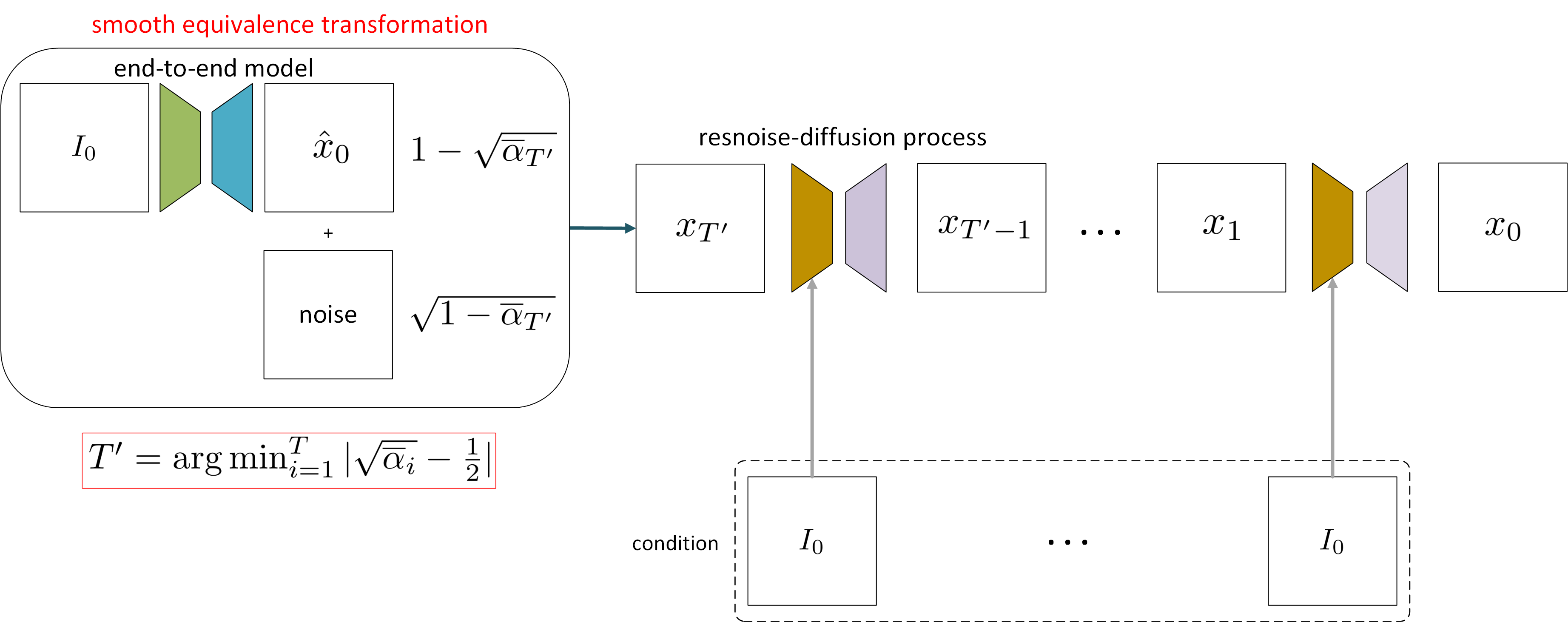
Figure 2: The inference pipeline of Resfusion . $I_{0}$ represents the input image, which goes through an $E2EModel$ to obtain the likelihood output $\hat{x}_{0}$. Then the resnoise-diffusion denoising process starts from the acceleration step $T^{\prime}$ we calculate in 27. According to 28, the posterior ${x}_{0}$ can be eliminated at $T^{\prime}$, thereby allowing the initialization of the inference process through $\hat{x}_{0}$. At each denoising step, $I_{0}$ is introduced as a condition for feature fusion, to better guide the diffusion direction. $x_{0}$ is the target image we Resfusion output.

3.1 Learning the resnoise between the likelihood output and ground truth

Image segmentation is a generation task to categorize the pixels in an image into different classes. End-to-end models for image segmentation aim to learn a likelihood distribution $P_{\psi}(x_{0})$ of segmentation masks $x_{0}$ through the source images $I_{0}$, as shown in 16, where $P_{data}$ represents the real distribution and $\psi$ represents the learnable parameters in end-to-end models.

$$P_{\psi}(x_{0})=\int P_{data}(I_{0})P_{\psi}(x_{0}|I_{0})dI_{0}$$ (16)

When the sampling space of $I_{0}$ and the parameter space of $\psi$ are large enough, with sufficient training, we can minimize $D_{KL}(P_{data}(x_{0})||P_{\psi}(x_{0}))$. If the end-to-end model is well-trained to fit this distribution, we can obtain the likelihood output $\hat{x}_{0}$ of real segmentation masks by utilizing the end-to-end model, as shown in 17. Here $E2EModel$ represents an end-to-end model, and $I_{0}$ represents the origin input image.

$$x_{0}\propto\hat{x}_{0}=E2EModel(I_{0})$$ (17)

However, there is a gap between ground truth $x_{0}$ and likelihood output $\hat{x}_{0}$, since the end-to-end model cannot completely fit the ground truth. We hope to use the diffusion process to close this gap. We define the residual term as 18.

$$R=\hat{x}_{0}-x_{0}$$ (18)

We can define $x_{t}$ as 19, where $\epsilon$ represents the Gaussian noise. We will provide a detailed explanation for why we embed $R$ to 5 in this way in Appendix A.2.

$${x}_{t}=\sqrt{\alpha_{t}}x_{t-1}+(1-\sqrt{\alpha_{t}})R+\sqrt{1-\alpha_{t}}\epsilon,\epsilon\sim N(0,I_{n\times n})$$ (19)

Similar to [21], ${x}_{t}$ can be reparameterized as 20.

$${x}_{t}=\sqrt{\overline{\alpha}_{t}}x_{0}+(1-\sqrt{\overline{\alpha}_{t}})R+\sqrt{1-\overline{\alpha}_{t}}\epsilon,\epsilon\sim N(0,I_{n\times n})$$ (20)

According to 20 and 18, we can derive 21.

$${x}_{t}=(2\sqrt{\overline{\alpha}_{t}}-1)x_{0}+(1-\sqrt{\overline{\alpha}_{t}})\hat{x}_{0}+\sqrt{1-\overline{\alpha}_{t}}\epsilon,\epsilon\sim N(0,I_{n\times n})$$ (21)

Then we can easily incorporate this likelihood estimation into vanilla Denoising Diffusion Probabilistic Models, following 22.

$$P_{\theta}(x_{0})=\int_{{x}_{1}:{x}_{T}}P_{data}({x}_{T})\prod_{t=1}^{T}P_{\theta}({x}_{t-1}|{x}_{t})d{x}_{1}:{x}_{T}$$ (22)

According to [21], the term to be minimized can be modified as 23, detailed proof can be found in Appendix A.1.

$$\mathbb{E}_{x_{0},\epsilon}[||(\epsilon+\frac{(1-\sqrt{\alpha_{t}})\sqrt{1-\overline{\alpha}_{t}}}{\beta_{t}}R)-\epsilon_{resnoise-\theta}(x_{t},t)||^{2}]$$ (23)

We introduce a residual noise, called resnoise, to describe the gap between ${x}_{t}$ and $x_{0}$, define as 24. Then 23 can be modified to 25.

$$\epsilon_{resnoise}=\epsilon+\frac{(1-\sqrt{\alpha_{t}})\sqrt{1-\overline{\alpha}_{t}}}{\beta_{t}}R$$ (24)

$$\begin{split}\mathbb{E}_{x_{0},\epsilon}[||\epsilon_{resnoise}-\epsilon_{resnoise-\theta}(x_{t},t)||^{2}]\end{split}$$ (25)

Through this process, we transform the learning of $\epsilon_{\theta}(x_{t},t)$ into $\epsilon_{resnoise-\theta}({x}_{t},t)$. $\epsilon_{\theta}(x_{t},t)$ learns the noise of the noisy ground truth. $\epsilon_{resnoise-\theta}({x}_{t},t)$ learns the resnoise between the likelihood noisy segmentation masks and the ground truth. We name this process resnoise-diffusion. The training process can be described as shown in Figure 1. The input $I_{0}$ served as a conditioning input will be discussed in section 3.3.

3.2 Using the likelihood output to accelerate train and inference process.

${x}_{T}$ is uncomputable because $x_{0}$ is unknown in 21, so we can not initialize ${x}_{T}$ directly.

However, $\hat{x}_{0}$ is computable. Fortunately, the $(2\sqrt{\overline{\alpha}_{t}}-1)$ before $x_{0}$ in 21 can be very close to zero. Then we can find a time step $T^{\prime}$, where $(2\sqrt{\overline{\alpha}_{t}}-1)$ is close to zero. So we can drive T’ as 26.

$$\sqrt{\overline{\alpha}_{T^{\prime}}}=\frac{1}{2}$$ (26)

When $T$ is sufficiently large, term $\sqrt{\overline{\alpha}_{t}}(t\leq T)$ is smooth. We call this process smooth equivalence transformation. Therefore, we can express $T^{\prime}$ as 27.

$$T^{\prime}=\arg\min_{i=1}^{T}|{\sqrt{\overline{\alpha}_{i}}}-\frac{1}{2}|$$ (27)

Then we can express ${x}_{T^{\prime}}$ as 28 with a very small bias when $T$ is sufficiently large.

$$x_{T^{\prime}}\approx(1-\sqrt{\overline{\alpha}_{T^{\prime}}})\hat{x}_{0}+\sqrt{1-\overline{\alpha}_{T^{\prime}}}\epsilon$$ (28)

Then we can modify 22 to 29, thus we only need to minimize 23 when $t\leq T^{\prime}$.

$$P_{\theta}(x_{0})=\int_{{x}_{1}:{x}_{T^{\prime}}}P_{data}({x}_{T^{\prime}})\prod_{t=1}^{T^{\prime}}P_{\theta}({x}_{t-1}|{x}_{t})d{x}_{1}:{x}_{T}$$ (29)

The reverse process is parameterized by $\theta$ and defined by 30.

$$P_{\theta}(x_{0:T^{\prime}-1}|x_{T^{\prime}})=\prod_{t=1}^{T^{\prime}}P_{\theta}(x_{t-1}|x_{t})$$ (30)

Starting from 28, the reverse process transforms the latent variable distribution into the data distribution $P_{\theta}(x_{0})$ according to [21]. The reverse process is performed by taking steps described by small Gaussian steps, as 31.

$$P_{\theta}(x_{t-1}|x_{t})=N(x_{t-1};\mu_{\theta}(x_{t},t),\Sigma_{\theta}(x_{t},t))$$ (31)

$$P_{\theta}(x_{0}|x_{1})=N(x_{0};\mu_{\theta}(x_{1},1))$$ (32)

According to [21], we can obtain 33.

$$\mu_{\theta}(x_{t},t)=\frac{1}{\sqrt{\alpha_{t}}}(x_{t}-\frac{\beta_{t}}{\sqrt{1-\overline{\alpha}_{t}}}\epsilon_{resnoise-\theta})$$ (33)

Resfusion $\mu_{\theta}$ predicts the resnoise $\epsilon_{resnoise-\theta}(x_{t},t)$, which is parameterized using 25. The inference process can be described as shown in Figure 2. The input $I_{0}$ served as a conditioning input will be discussed in section 3.3.

3.3 Generating segmentation masks from coarse to fine

Similar to the approach proposed by Amit et al. [2] in their work on segmentation with diffusion, our method enhances the diffusion model by incorporating a conditioning function during the denoising steps. This function integrates latent representation from both the current estimate $x_{t}$ and the input image $I_{0}$.

Then 25 can be modified to 34.

$$\begin{split}\mathbb{E}_{x_{0},\epsilon,t}[||\epsilon_{resnoise}-\epsilon_{resnoise-\theta}((x_{t},I_{0},t)||^{2}]\end{split}$$ (34)

Based on the derivations from the section 3.1 and section 3.2, the training and inference processes of Resfusion can be represented as Algorithm 1 and 2.

Algorithm 1 Training Algorithm for Resnoise Learning

0:  total diffusion steps $T$, images and segmentation masks dataset $D={(I_{0}^{n},x_{0}^{n})}_{n}^{N}$, pretrained end-to-end model $E2EModel$.

  $\beta_{t}=\frac{10^{-4}(T-t)+2\times 10^{-2}(t-1)}{T-1}$

  $\alpha_{t}=1-\beta_{t}$

  $\overline{\alpha}_{t}={\textstyle\prod_{s=1}^{t}}\alpha_{s}$

  $T^{\prime}=\arg\min_{i=1}^{T}|{\sqrt{\overline{\alpha}_{i}}}-\frac{1}{2}|$

  repeat

     Sample $(I_{0}^{i},x_{0}^{i})\sim D,\epsilon\sim N(0,I_{n\times n})$

     Sample $t\sim Uniform({1,...,T^{\prime}})$

     $\hat{x}_{0}=E2EModel(I_{0})$ {no gradient and can be cached}

     $R=\hat{x}_{0}-x_{0}$

     ${x}_{t}=\sqrt{\overline{\alpha}_{t}}x_{0}+(1-\sqrt{\overline{\alpha}_{t}})R+\sqrt{1-\overline{\alpha}_{t}}\epsilon$

     $\epsilon_{resnoise}=\epsilon+\frac{(1-\sqrt{\alpha_{t}})\sqrt{1-\overline{\alpha}_{t}}}{\beta_{t}}R$

     take gradient step on

      $\nabla_{\theta}||\epsilon_{resnoise}-\epsilon_{resnoise-\theta}({x}_{t},I_{0},t)||$

  until convergence

Algorithm 2 Inference Algorithm for Resfusion

0:  total diffusion steps $T$, image $I_{0}$, pretrained end-to-end model $E2EModel$, pretrained Resfusion model $\epsilon_{resnoise-\theta}$.

  $\beta_{t}=\frac{10^{-4}(T-t)+2\times 10^{-2}(t-1)}{T-1}$

  $\alpha_{t}=1-\beta_{t}$

  $\overline{\alpha}_{t}={\textstyle\prod_{s=1}^{t}}\alpha_{s}$

  $\widetilde{\beta}_{t}=\frac{1-\overline{\alpha}_{t-1}}{1-\overline{\alpha}_{t}}\beta_{t}$

  $T^{\prime}=\arg\min_{i=1}^{T}|{\sqrt{\overline{\alpha}_{i}}}-\frac{1}{2}|$

  Sample $\epsilon\sim N(0,I_{n\times n})$

  $\hat{x}_{0}=E2EModel(I_{0})$

  $x_{T^{\prime}}=(1-\sqrt{\overline{\alpha}_{T^{\prime}}})\hat{x}_{0}+\sqrt{1-\overline{\alpha}_{T^{\prime}}}\epsilon$

  for $t=T^{\prime},T^{\prime}-1,...,2$ do

     Sample $z\sim N(0,I_{n\times n})$

     $x_{t-1}=\frac{1}{\sqrt{\alpha_{t}}}(x_{t}-\frac{\beta_{t}}{\sqrt{1-\overline{\alpha}_{t}}}(\epsilon_{resnoise-\theta}(x_{t},I_{0},t))+\sqrt{\widetilde{\beta}}z$

  end for

  return  $x_{0}=\frac{1}{\sqrt{\alpha_{1}}}(x_{1}-\frac{\beta_{1}}{\sqrt{1-\overline{\alpha}_{1}}}\epsilon_{resnoise-\theta}(x_{1},I_{0},1))$

Just like the vanilla Denoising Diffusion Probabilistic Models (DDPM), Resfusion gradually fit $\hat{x}_{t}$ to $x_{0}$ in an autoregressive manner, implicitly reducing the residual term between ${x}_{T}$ and $x_{0}$ with resnoise. Since $\hat{x}_{0}$ can be cached, the process of obtaining $\hat{x}_{0}$ does not increase the training time.

Step $T^{\prime}$ is non-trivial, since $x_{T^{\prime}}$ is very close to $\hat{x}_{T^{\prime}}$ at step $T^{\prime}$ when we defined $\hat{x}_{t}$ as 35 with the same Gaussian noise $\epsilon$. We essentially quantitatively computed the accelerated step $T^{\prime}$. When T is large enough, the approximate equal sign will become an equal sign. The determination of step $T^{\prime}$ corresponds to the point where the posterior probability distribution becomes indistinguishable from the prior probability distribution.

$$\hat{x}_{t}=\sqrt{\overline{\alpha}_{t}}\hat{x}_{0}+\sqrt{1-\overline{\alpha}_{t}}\epsilon$$ (35)

$$\sqrt{\overline{\alpha}_{T^{\prime}}}\approx 1-\sqrt{\overline{\alpha}_{T^{\prime}}}$$ (36)

$$x_{T^{\prime}}\approx\hat{x}_{T^{\prime}}$$ (37)

It is important to note that Resfusion is not limited to image segmentation. It can be applied to any image generation domain. The versatility of our framework lies in its ability to combine end-to-end models and denoising diffusion models.

Following [21] we set

$$\Sigma_{\theta}(x_{t},t)=\sigma_{t}^{2}I_{n\times n}$$ (38)

where

$$\widetilde{\beta}_{t}=\frac{1-\overline{\alpha}_{t-1}}{1-\overline{\alpha}_{t}}\beta_{t}$$ (39)

$$\sigma_{t}^{2}=\widetilde{\beta}_{t}$$ (40)

The forward process variance parameter is a linearly increasing constant from $\beta_{1}=10^{-4}$ to $\beta_{T}=2\times 10^{-2}$. $\beta_{t}$ can be formally represented as 41.

$$\beta_{t}=\frac{10^{-4}(T-t)+2\times 10^{-2}(t-1)}{T-1}$$ (41)

4 Evaluation

Detailed comparative experiments and ablation experiments on image segmentation will be released. Detailed comparative experiments in the fields of image denoising, image restoration, image dehazing, and image deraining will also be released. Detailed scale experiments will be released.

5 Related Work

The diffusion process is a Markov process in which the original data is gradually corrupted by noise and eventually transforms into pure Gaussian noise. Subsequently, the denoising model learns the reverse diffusion process with the aim of gradually recovering the original data. Sohl-Dickstein et al. [42] first proposed diffusion models for mapping the disrupted data to a noise distribution. Ho et al. [21] subsequently demonstrated that this modeling approach is akin to score-matching models, which belong to a class of models that estimate the gradient of the log-density. This concept aligns with the foundations of score-matching models as previously described by Hyvärinen and Dayan [22], Vincent [48], Song and Ermon [44, 45]. This development led to a more simplified variational lower bound training objective and a denoising diffusion probabilistic model (DDPM) as presented by Ho et al. [21]. DDPM achieved state-of-the-art performance for unconditional image generation, particularly on datasets like CIFAR-10. However, in practical applications, DDPMs were found to be suboptimal in terms of log-likelihood estimation. This limitation was addressed by Nichol and Dhariwal [37] through the introduction of a learnable variance schedule, a sinusoidal noise schedule and the sampling for time steps. It’s worth noting that diffusion models are typically trained with hundreds or even thousands of steps, and performing inference with the same number of steps can be time-consuming. As a result, various strategies have been proposed to enable faster sampling in these models. Song et al. [43] introduced a deterministic model known as the denoising diffusion implicit model (DDIM). DDIM shares the same marginal distribution as DDPM. Building upon this, Liu et al. [31] further extended the reverse step of DDIM by formulating it as an ordinary differential equation. They used high-order numerical techniques, such as the Runge-Kutta method, in combination with predicted noise to facilitate sampling with second-order convergence. Additionally, Zheng et al. [64] and Lyu et al. [34] have proposed strategies to expedite the training of diffusion models. These approaches involve shortening the noise schedule and focusing on a truncated diffusion chain with reduced noise levels, making the training process more efficient. Based on the aforementioned improvements, various tasks of image generation utilize denoising diffusion models as foundational framework, including DALL·E 2[39], stable diffusion and Midjourney[40].

Due to the impressive feature extraction capabilities of denoising diffusion models, several researchers have fine-tuned these models and harnessed their encoding and decoding capabilities for segmentation tasks. Baranchuk et al. [5] extracted representations from the intermediate layers of the diffusion model as the basis for pixel-level segmentation. Rousseau et al. [41] regarded the denoising process as a pre-training procedure, fine-tuning the denoising diffusion model for Dental Radiography segmentation. Ni et al. [36] utilized fine-grained multimodal information from the generative model for Zero-shot Referring Image Segmentation. Wu et al. [58] generated pixel-level pseudo-labels by utilizing the cross-attention map of the intermediate features in the denoising diffusion model. Tian et al. [47] iteratively generates semantic segmentation masks using the attention map of the intermediate feature layer in stable-diffusion. Tan et al. [46] employed denoising diffusion models for data augmentation in Few-Shot Semantic Segmentation. The above methods mainly focus on utilizing the powerful feature extraction capability of the diffusion model and fine-tuning the model for application in end-to-end models, rather than directly applying the denoising diffusion process to the field of segmentation.

Amit et al. [2] first introduce the step-wise denoising process of diffusion denoising models into the field of image segmentation. A series of studies emerged to modify and refine this process, encompassing adjustments in architecture[38, 3, 54, 62], improvements in the training procedure[14, 9, 13], enhancements to the denoising modules[49, 59, 55, 7, 57, 12], acceleration of the inference process[18, 17], and application to downstream tasks[35, 1, 24, 4, 23]. Fu et al. [14], Fu et al. [13], Wang et al. [49], Lai et al. [28], [9] and Watson et al. [53] transformed the process of predicting noise into predicting masks. However, in each inference step, it is required to generate a predicted mask, incorporate it into the noise to generate a new predicted mask, and repeat the noise. This ”renoise” process significantly increases the inference time.

Chen et al. [10] formulated panoptic segmentation as a discrete data generation problem and proposed a general diffusion architecture to model panoramic masks and is capable of automatically modeling videos. Chen et al. [11] generated segmentation masks gradually by interacting with prompts during the denoising diffusion procedure. Kim et al. [25] integrated generative adversarial networks with denoising diffusion models for vessel segmentation. Zhang et al. [63] achieves a synchronous diffusion process by incorporating shared noise. Zhou et al. [65] proposed a Diffusion-based and Prototype-guided network for unsupervised domain adaptive segmentation. Bieder et al. [6] contributed a memory-efficient patch-based diffusion model called PatchDDM, which is designed to reduce the memory consumption of the denoising diffusion models. Kirkegaard [27] proposed an instance segmentation method based on the diffusion model, which spontaneously breaks the inherent symmetry that semantic-similar objects must produce different outputs, while allowing for overlapping labels.

Although these studies have made improvements to the vanilla denoising diffusion model for image segmentation, there is no method that can seamlessly combine the existing end-to-end methods with the denoising diffusion models. We propose the Resfusion architecture, a method that gradually generates target images in a coarse-to-fine manner, seamlessly integrating current state-of-the-art end-to-end models and denoising diffusion models.

6 Conclusion

By learning the resnoise between the likelihood output and ground truth and using the likelihood output to accelerate the training and inference process, we propose the Resfusion , a framework that gradually generates target images in a coarse-to-fine manner, seamlessly integrating current state-of-the-art end-to-end models and denoising diffusion models.

By introducing a novel resnoise-diffusion process, we aim to bridge the gap between the likelihood output and ground truth output using a Markov process. By learning the resnoise between the likelihood output and ground truth output, We unified the training and inference denoising processes through resnoise-diffusion. Our framework, Resfusion , seamlessly integrates state-of-the-art end-to-end models and denoising diffusion models.

By employing a novel technique called ”smooth equivalence transformation” during the resnoise-diffusion process, we identify the ideal acceleration step $T^{\prime}$. As the total steps $T$ increases sufficiently, the bias tends to converge to zero. The determination of step $T^{\prime}$ is crucial since it corresponds to the point where the posterior probability distribution becomes indistinguishable from the prior probability distribution.

It is important to note that Resfusion is not limited to image segmentation. It can be applied to any image generation domain. The versatility of our framework lies in its ability to combine end-to-end models and denoising diffusion models. Our subsequent experiments have demonstrated that Resfusion can be easily applied to various image generation tasks and exhibits strong competitiveness.

Appendix A Appendix Section

A.1 Detailed Proof

According to 19 and 20, the q-sampling process can be written as 42 and 43.

$$q(x_{t}|x_{t-1})=\mathcal{N}(x_{t};\sqrt{\alpha_{t}}x_{t-1}+(1-\sqrt{\alpha_{t}})R,(1-\alpha_{t})I)$$ (42)

$$q(x_{t}|x_{0})=\mathcal{N}(x_{t};\sqrt{\overline{\alpha}_{t}}x_{0}+(1-\sqrt{\overline{\alpha}_{t}})R,(1-\overline{\alpha}_{t})I)$$ (43)

Similar to [33] equation [73]-[84],

$$q(x_{t-1}|x_{t},x_{0})$$ (44)

$$=\frac{q(x_{t}|x_{t-1},x_{0})q(x_{t-1}|x_{0})}{q(x_{t}|x_{0})}$$

$$=\frac{\mathcal{N}(x_{t};\sqrt{\alpha_{t}}x_{t-1}+(1-\sqrt{\alpha_{t}})R,(1-\alpha_{t})I)\mathcal{N}(x_{t-1};\sqrt{\overline{\alpha}_{t-1}}x_{0}+(1-\sqrt{\overline{\alpha}_{t-1}})R,(1-\overline{\alpha}_{t-1})I)}{\mathcal{N}(x_{t};\sqrt{\overline{\alpha}_{t}}x_{0}+(1-\sqrt{\overline{\alpha}_{t}})R,(1-\overline{\alpha}_{t})I)}$$

$$\propto exp\{-[\frac{[x_{t}-(\sqrt{\alpha_{t}}x_{t-1}+(1-\sqrt{\alpha_{t}})R)]^{2}}{2(1-\alpha_{t})}+\frac{[x_{t-1}-(\sqrt{\overline{\alpha}_{t-1}}x_{0}+(1-\sqrt{\overline{\alpha}_{t-1}})R)]^{2}}{2(1-\overline{\alpha}_{t-1})}-\frac{[x_{t}-(\sqrt{\overline{\alpha}_{t}}x_{0}+(1-\sqrt{\overline{\alpha}_{t}})R)]^{2}}{2(1-\overline{\alpha}_{t})}]\}$$

$$=exp\{-[\frac{[(x_{t}-R)-\sqrt{\alpha_{t}}(x_{t-1}-R)]^{2}}{2(1-\alpha_{t})}+\frac{[(x_{t-1}-R)-\sqrt{\overline{\alpha}_{t-1}}(x_{0}-R)]^{2}}{2(1-\overline{\alpha}_{t-1})}-\frac{[(x_{t}-R)-\sqrt{\overline{\alpha}_{t}}(x_{0}-R)]^{2}}{2(1-\overline{\alpha}_{t})}]\}$$

$$\propto\mathcal{N}(x_{t-1}-R;\frac{\sqrt{\alpha_{t}}(1-\overline{\alpha}_{t-1})(x_{t}-R)+\sqrt{\overline{\alpha}_{t-1}}(1-\alpha_{t})(x_{0}-R)}{1-\overline{\alpha}_{t}},\widetilde{\beta}_{t}I)$$

$$\propto\mathcal{N}(x_{t-1};\frac{\sqrt{\alpha_{t}}(1-\overline{\alpha}_{t-1})(x_{t}-R)+\sqrt{\overline{\alpha}_{t-1}}(1-\alpha_{t})(x_{0}-R)}{1-\overline{\alpha}_{t}}+R,\widetilde{\beta}_{t}I)$$

Then we can define $\widetilde{\mu}(x_{t},x_{0})$ as 45.

$$\widetilde{\mu}(x_{t},x_{0})=\frac{\sqrt{\overline{\alpha}_{t-1}}\beta_{t}}{1-\overline{\alpha}_{t}}(x_{0}-R)+\frac{\sqrt{\alpha_{t}}(1-\overline{\alpha}_{t-1})}{1-\overline{\alpha}_{t}}(x_{t}-R)+R$$ (45)

We can derive 46 through 20.

$$x_{t}-R=\sqrt{\overline{\alpha}_{t}}(x_{0}-R)+\sqrt{1-\overline{\alpha}_{t}}\epsilon,\epsilon\sim N(0,I_{n\times n})$$ (46)

Similar to [33] equation $[116]-[124]$, we can derive 47 through 46.

$$L_{t-1}-C =\mathbb{E}_{x_{0},\epsilon,t}[\frac{1}{2\sigma_{t}^{2}}||\widetilde{\mu}(x_{t},x_{0})-\mu_{\theta}(x_{t}(x_{0},\epsilon,R),t)||^{2}]$$ (47)

$$=\mathbb{E}_{x_{0},\epsilon,t}[\frac{1}{2\sigma_{t}^{2}}||\{\frac{1}{\sqrt{\alpha_{t}}}[(x_{t}(x_{0},\epsilon,R)-R)-\frac{\beta_{t}}{\sqrt{1-\overline{\alpha}_{t}}}\epsilon]+R\}-\mu_{\theta}(x_{t}(x_{0},\epsilon,R),t)||^{2}]$$

According to 48, we can modify 47 as 49.

$$\frac{1}{\sqrt{\alpha_{t}}}(x_{t}-R-\frac{\beta_{t}}{\sqrt{1-\overline{\alpha}_{t}}}\epsilon)+R =\frac{1}{\sqrt{\alpha_{t}}}(x_{t}-R+\sqrt{\alpha_{t}}R-\frac{\beta_{t}}{\sqrt{1-\overline{\alpha}_{t}}}\epsilon)$$ (48)

$$=\frac{1}{\sqrt{\alpha_{t}}}(x_{t}-(1-\sqrt{\alpha_{t}})R-\frac{\beta_{t}}{\sqrt{1-\overline{\alpha}_{t}}}\epsilon)$$

$$=\frac{1}{\sqrt{\alpha_{t}}}(x_{t}-\frac{(1-\sqrt{\alpha_{t}})\sqrt{1-\overline{\alpha}_{t}}}{\beta_{t}}\frac{\beta_{t}}{\sqrt{1-\overline{\alpha}_{t}}}R-\frac{\beta_{t}}{\sqrt{1-\overline{\alpha}_{t}}}\epsilon)$$

$$=\frac{1}{\sqrt{\alpha_{t}}}[x_{t}-\frac{\beta_{t}}{\sqrt{1-\overline{\alpha}_{t}}}(\epsilon+\frac{(1-\sqrt{\alpha_{t}})\sqrt{1-\overline{\alpha}_{t}}}{\beta_{t}}R)]$$

$$L_{t-1}-C=\mathbb{E}_{x_{0},\epsilon,t}[\frac{1}{2\sigma_{t}^{2}}||\frac{1}{\sqrt{\alpha_{t}}}[x_{t}(x_{0},\epsilon,R)-\frac{\beta_{t}}{\sqrt{1-\overline{\alpha}_{t}}}(\epsilon+\frac{(1-\sqrt{\alpha_{t}})\sqrt{1-\overline{\alpha}_{t}}}{\beta_{t}}R)]-\mu_{\theta}(x_{t}(x_{0},\epsilon,R),t)||^{2}]$$ (49)

According to [21], the minimize term become 23.

A.2 Working principle

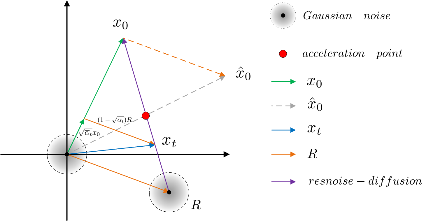
Figure 3: working principle of Resfusion .

${x}_{0}$ represents the ground truth distribution, while $\hat{x}_{0}$ represents the likelihood output generated by the $E2EModel$. $\hat{x}_{0}-{x}_{0}$ represents the gap between them, defined as the residual term $R$ in 18. Resfusion does not explicitly guide $\hat{x}_{0}$ to align directly with ${x}_{0}$. Instead, it indirectly learns the distribution of $R$ by denoising $x_{t}$ to $x_{0}$ through resnoise-diffusion. The resnoise-diffusion guiding ${x}_{t}$ gradually towards ${x}_{0}$ along this direction. Following the principles of similar triangles, the coefficient of $R$ is computed as $1-\sqrt{\overline{\alpha}_{t}}$. At any $t$ step during the training process, ${x}_{t}$ is calculated based on ${x}_{0}$ and $R$ through 19.

We assume that the residual $R$ follows truncated normal distribution $\psi(0,I_{n\times n},-2,2)$, where [-2, 2] is the truncated interval. In this case, the state of $R$ is independent of $x_{0}$, and thus $x_{t}$ in 19 is only related to $x_{t-1}$, which means 19 represents a Markov process. Therefore, resnoise-diffusion can be imagined as doing diffusion from $R$ to $x_{0}$.

Resnoise-diffusion intersects with vanilla DDPM from origin point (which is (0,0) in two-dimensional plane) to $\hat{x}_{0}$, at which point the two processes are in the same state. Thus, the intersection can be regarded as acceleration point. The intersection point of two diagonals of a parallelogram is the midpoint of them, but due to the discrete nature of the diffusion process, the acceleration point actually falls on the point closest to the intersection, which is $T^{\prime}$ as 27. Meanwhile, since $x_{T^{\prime}}$ is available, diffusion steps after $T^{\prime}$ are not necessary according to 29. Therefore, Resfusion can be directly started from $T^{\prime}$ for both inference and training process. The vanilla DDPM is deterministic because $\hat{x}_{0}$ is available during inference, and the intersection of these two processes is the acceleration point.

References

- Alimanov and Islam [2023] Alnur Alimanov and Md Baharul Islam. Denoising diffusion probabilistic model for retinal image generation and segmentation. In 2023 IEEE International Conference on Computational Photography (ICCP), pages 1–12. IEEE, 2023.
- Amit et al. [2021] Tomer Amit, Tal Shaharbany, Eliya Nachmani, and Lior Wolf. Segdiff: Image segmentation with diffusion probabilistic models. arXiv preprint arXiv:2112.00390, 2021.
- Amit et al. [2023] Tomer Amit, Shmuel Shichrur, Tal Shaharabany, and Lior Wolf. Annotator consensus prediction for medical image segmentation with diffusion models. arXiv preprint arXiv:2306.09004, 2023.
- Ayala et al. [2023] C Ayala, R Sesma, C Aranda, and M Galar. Diffusion models for remote sensing imagery semantic segmentation. In IGARSS 2023-2023 IEEE International Geoscience and Remote Sensing Symposium, pages 5654–5657. IEEE, 2023.
- Baranchuk et al. [2021] Dmitry Baranchuk, Ivan Rubachev, Andrey Voynov, Valentin Khrulkov, and Artem Babenko. Label-efficient semantic segmentation with diffusion models. arXiv preprint arXiv:2112.03126, 2021.
- Bieder et al. [2023] Florentin Bieder, Julia Wolleb, Alicia Durrer, Robin Sandkuehler, and Philippe C Cattin. Memory-efficient 3d denoising diffusion models for medical image processing. In Medical Imaging with Deep Learning, 2023.
- Bozorgpour et al. [2023] Afshin Bozorgpour, Yousef Sadegheih, Amirhossein Kazerouni, Reza Azad, and Dorit Merhof. Dermosegdiff: A boundary-aware segmentation diffusion model for skin lesion delineation. In International Workshop on PRedictive Intelligence In MEdicine, pages 146–158. Springer, 2023.
- Cao et al. [2020] Jiale Cao, Hisham Cholakkal, Rao Muhammad Anwer, Fahad Shahbaz Khan, Yanwei Pang, and Ling Shao. D2det: Towards high quality object detection and instance segmentation. In Proceedings of the IEEE/CVF conference on computer vision and pattern recognition, pages 11485–11494, 2020.
- Chen et al. [2022] Ting Chen, Ruixiang Zhang, and Geoffrey Hinton. Analog bits: Generating discrete data using diffusion models with self-conditioning. arXiv preprint arXiv:2208.04202, 2022.
- Chen et al. [2023] Ting Chen, Lala Li, Saurabh Saxena, Geoffrey Hinton, and David J Fleet. A generalist framework for panoptic segmentation of images and videos. In Proceedings of the IEEE/CVF International Conference on Computer Vision, pages 909–919, 2023.
- Chen et al. [2021] Xi Chen, Zhiyan Zhao, Feiwu Yu, Yilei Zhang, and Manni Duan. Conditional diffusion for interactive segmentation. In Proceedings of the IEEE/CVF International Conference on Computer Vision, pages 7345–7354, 2021.
- Chowdary and Yin [2023] G Jignesh Chowdary and Zhaozheng Yin. Diffusion transformer u-net for medical image segmentation. In International Conference on Medical Image Computing and Computer-Assisted Intervention, pages 622–631. Springer, 2023.
- Fu et al. [2023a] Yunguan Fu, Yiwen Li, Shaheer U Saeed, Matthew J Clarkson, and Yipeng Hu. Importance of aligning training strategy with evaluation for diffusion models in 3d multiclass segmentation. arXiv preprint arXiv:2303.06040, 2023a.
- Fu et al. [2023b] Yunguan Fu, Yiwen Li, Shaheer U Saeed, Matthew J Clarkson, and Yipeng Hu. A recycling training strategy for medical image segmentation with diffusion denoising models. arXiv preprint arXiv:2308.16355, 2023b.
- Ghouse et al. [2023] Noor Fathima Ghouse, Jens Petersen, Auke Wiggers, Tianlin Xu, and Guillaume Sautière. A residual diffusion model for high perceptual quality codec augmentation, 2023.
- Goodfellow et al. [2020] Ian Goodfellow, Jean Pouget-Abadie, Mehdi Mirza, Bing Xu, David Warde-Farley, Sherjil Ozair, Aaron Courville, and Yoshua Bengio. Generative adversarial networks. Communications of the ACM, 63(11):139–144, 2020.
- Guo et al. [2023a] Xinyu Guo, Zhouqian Wang, Huaying Hao, Qinxiang Zheng, Jiong Zhang, Wei Chen, and Yitian Zhao. Structure constrained diffusion models for pterygium segmentation. In 2023 IEEE 20th International Symposium on Biomedical Imaging (ISBI), pages 1–5. IEEE, 2023a.
- Guo et al. [2023b] Xutao Guo, Yanwu Yang, Chenfei Ye, Shang Lu, Bo Peng, Hua Huang, Yang Xiang, and Ting Ma. Accelerating diffusion models via pre-segmentation diffusion sampling for medical image segmentation. In 2023 IEEE 20th International Symposium on Biomedical Imaging (ISBI), pages 1–5. IEEE, 2023b.
- He et al. [2017] Kaiming He, Georgia Gkioxari, Piotr Dollár, and Ross Girshick. Mask r-cnn. In Proceedings of the IEEE international conference on computer vision, pages 2961–2969, 2017.
- Ho and Salimans [2022] Jonathan Ho and Tim Salimans. Classifier-free diffusion guidance. arXiv preprint arXiv:2207.12598, 2022.
- Ho et al. [2020] Jonathan Ho, Ajay Jain, and Pieter Abbeel. Denoising diffusion probabilistic models. Advances in neural information processing systems, 33:6840–6851, 2020.
- Hyvärinen and Dayan [2005] Aapo Hyvärinen and Peter Dayan. Estimation of non-normalized statistical models by score matching. Journal of Machine Learning Research, 6(4), 2005.
- Ivanovska et al. [2023] Marija Ivanovska, Vitomir Štruc, and Janez Perš. Tomatodiff: On–plant tomato segmentation with denoising diffusion models. In 2023 18th International Conference on Machine Vision and Applications (MVA), pages 1–6. IEEE, 2023.
- Jiang and Mu [2023] Borui Jiang and Yadong Mu. Diffused fourier network for video action segmentation. In Proceedings of the 31st ACM International Conference on Multimedia, pages 5474–5483, 2023.
- Kim et al. [2022] Boah Kim, Yujin Oh, and Jong Chul Ye. Diffusion adversarial representation learning for self-supervised vessel segmentation. arXiv preprint arXiv:2209.14566, 2022.
- Kirillov et al. [2019] Alexander Kirillov, Kaiming He, Ross Girshick, Carsten Rother, and Piotr Dollár. Panoptic segmentation. In Proceedings of the IEEE/CVF conference on computer vision and pattern recognition, pages 9404–9413, 2019.
- Kirkegaard [2023] Julius B Kirkegaard. Spontaneous breaking of symmetry in overlapping cell instance segmentation using diffusion models. bioRxiv, pages 2023–07, 2023.
- Lai et al. [2023] Zeqiang Lai, Yuchen Duan, Jifeng Dai, Ziheng Li, Ying Fu, Hongsheng Li, Yu Qiao, and Wenhai Wang. Denoising diffusion semantic segmentation with mask prior modeling. arXiv preprint arXiv:2306.01721, 2023.
- Liu et al. [2023a] Baolin Liu, Zongyuan Yang, Pengfei Wang, Junjie Zhou, Ziqi Liu, Ziyi Song, Yan Liu, and Yongping Xiong. Textdiff: Mask-guided residual diffusion models for scene text image super-resolution. arXiv preprint arXiv:2308.06743, 2023a.
- Liu et al. [2023b] Jiawei Liu, Qiang Wang, Huijie Fan, Yinong Wang, Yandong Tang, and Liangqiong Qu. Residual denoising diffusion models. arXiv preprint arXiv:2308.13712, 2023b.
- Liu et al. [2022] Luping Liu, Yi Ren, Zhijie Lin, and Zhou Zhao. Pseudo numerical methods for diffusion models on manifolds. arXiv preprint arXiv:2202.09778, 2022.
- Long et al. [2015] Jonathan Long, Evan Shelhamer, and Trevor Darrell. Fully convolutional networks for semantic segmentation. In Proceedings of the IEEE conference on computer vision and pattern recognition, pages 3431–3440, 2015.
- Luo [2022] Calvin Luo. Understanding diffusion models: A unified perspective. arXiv preprint arXiv:2208.11970, 2022.
- Lyu et al. [2022] Zhaoyang Lyu, Xudong Xu, Ceyuan Yang, Dahua Lin, and Bo Dai. Accelerating diffusion models via early stop of the diffusion process. arXiv preprint arXiv:2205.12524, 2022.
- Mao et al. [2023] Yuxin Mao, Jing Zhang, Mochu Xiang, Yunqiu Lv, Yiran Zhong, and Yuchao Dai. Contrastive conditional latent diffusion for audio-visual segmentation. arXiv preprint arXiv:2307.16579, 2023.
- Ni et al. [2023] Minheng Ni, Yabo Zhang, Kailai Feng, Xiaoming Li, Yiwen Guo, and Wangmeng Zuo. Ref-diff: Zero-shot referring image segmentation with generative models. arXiv preprint arXiv:2308.16777, 2023.
- Nichol and Dhariwal [2021] Alexander Quinn Nichol and Prafulla Dhariwal. Improved denoising diffusion probabilistic models. In International Conference on Machine Learning, pages 8162–8171. PMLR, 2021.
- Rahman et al. [2023] Aimon Rahman, Jeya Maria Jose Valanarasu, Ilker Hacihaliloglu, and Vishal M Patel. Ambiguous medical image segmentation using diffusion models. In Proceedings of the IEEE/CVF Conference on Computer Vision and Pattern Recognition, pages 11536–11546, 2023.
- Ramesh et al. [2022] Aditya Ramesh, Prafulla Dhariwal, Alex Nichol, Casey Chu, and Mark Chen. Hierarchical text-conditional image generation with clip latents. arXiv preprint arXiv:2204.06125, 1(2):3, 2022.
- Rombach et al. [2022] Robin Rombach, Andreas Blattmann, Dominik Lorenz, Patrick Esser, and Björn Ommer. High-resolution image synthesis with latent diffusion models. In Proceedings of the IEEE/CVF conference on computer vision and pattern recognition, pages 10684–10695, 2022.
- Rousseau et al. [2023] Jérémy Rousseau, Christian Alaka, Emma Covili, Hippolyte Mayard, Laura Misrachi, and Willy Au. Pre-training with diffusion models for dental radiography segmentation. arXiv preprint arXiv:2307.14066, 2023.
- Sohl-Dickstein et al. [2015] Jascha Sohl-Dickstein, Eric Weiss, Niru Maheswaranathan, and Surya Ganguli. Deep unsupervised learning using nonequilibrium thermodynamics. In International conference on machine learning, pages 2256–2265. PMLR, 2015.
- Song et al. [2020] Jiaming Song, Chenlin Meng, and Stefano Ermon. Denoising diffusion implicit models. arXiv preprint arXiv:2010.02502, 2020.
- Song and Ermon [2019] Yang Song and Stefano Ermon. Generative modeling by estimating gradients of the data distribution. Advances in neural information processing systems, 32, 2019.
- Song and Ermon [2020] Yang Song and Stefano Ermon. Improved techniques for training score-based generative models. Advances in neural information processing systems, 33:12438–12448, 2020.
- Tan et al. [2023] Weimin Tan, Siyuan Chen, and Bo Yan. Diffss: Diffusion model for few-shot semantic segmentation. arXiv preprint arXiv:2307.00773, 2023.
- Tian et al. [2023] Junjiao Tian, Lavisha Aggarwal, Andrea Colaco, Zsolt Kira, and Mar Gonzalez-Franco. Diffuse, attend, and segment: Unsupervised zero-shot segmentation using stable diffusion. arXiv preprint arXiv:2308.12469, 2023.
- Vincent [2011] Pascal Vincent. A connection between score matching and denoising autoencoders. Neural computation, 23(7):1661–1674, 2011.
- Wang et al. [2023a] Hefeng Wang, Jiale Cao, Rao Muhammad Anwer, Jin Xie, Fahad Shahbaz Khan, and Yanwei Pang. Dformer: Diffusion-guided transformer for universal image segmentation. arXiv preprint arXiv:2306.03437, 2023a.
- Wang et al. [2023b] Jinglong Wang, Xiawei Li, Jing Zhang, Qingyuan Xu, Qin Zhou, Qian Yu, Lu Sheng, and Dong Xu. Diffusion model is secretly a training-free open vocabulary semantic segmenter. arXiv preprint arXiv:2309.02773, 2023b.
- Wang et al. [2022] Wenguan Wang, James Liang, and Dongfang Liu. Learning equivariant segmentation with instance-unique querying. Advances in Neural Information Processing Systems, 35:12826–12840, 2022.
- Wang et al. [2020] Xinlong Wang, Rufeng Zhang, Tao Kong, Lei Li, and Chunhua Shen. Solov2: Dynamic and fast instance segmentation. Advances in Neural information processing systems, 33:17721–17732, 2020.
- Watson et al. [2023] Joseph L Watson, David Juergens, Nathaniel R Bennett, Brian L Trippe, Jason Yim, Helen E Eisenach, Woody Ahern, Andrew J Borst, Robert J Ragotte, Lukas F Milles, et al. De novo design of protein structure and function with rfdiffusion. Nature, 620(7976):1089–1100, 2023.
- Wolleb et al. [2022] Julia Wolleb, Robin Sandkühler, Florentin Bieder, Philippe Valmaggia, and Philippe C Cattin. Diffusion models for implicit image segmentation ensembles. In International Conference on Medical Imaging with Deep Learning, pages 1336–1348. PMLR, 2022.
- Wu et al. [2022a] Junde Wu, Rao Fu, Huihui Fang, Yu Zhang, Yehui Yang, Haoyi Xiong, Huiying Liu, and Yanwu Xu. Medsegdiff: Medical image segmentation with diffusion probabilistic model. arXiv preprint arXiv:2211.00611, 2022a.
- Wu et al. [2022b] Junfeng Wu, Yi Jiang, Song Bai, Wenqing Zhang, and Xiang Bai. Seqformer: Sequential transformer for video instance segmentation. In European Conference on Computer Vision, pages 553–569. Springer, 2022b.
- Wu et al. [2023a] Junde Wu, Rao Fu, Huihui Fang, Yu Zhang, and Yanwu Xu. Medsegdiff-v2: Diffusion based medical image segmentation with transformer. arXiv preprint arXiv:2301.11798, 2023a.
- Wu et al. [2023b] Weijia Wu, Yuzhong Zhao, Mike Zheng Shou, Hong Zhou, and Chunhua Shen. Diffumask: Synthesizing images with pixel-level annotations for semantic segmentation using diffusion models. arXiv preprint arXiv:2303.11681, 2023b.
- Xing et al. [2023] Zhaohu Xing, Liang Wan, Huazhu Fu, Guang Yang, and Lei Zhu. Diff-unet: A diffusion embedded network for volumetric segmentation. arXiv preprint arXiv:2303.10326, 2023.
- Yang et al. [2023] Zongyuan Yang, Baolin Liu, Yongping Xxiong, Lan Yi, Guibin Wu, Xiaojun Tang, Ziqi Liu, Junjie Zhou, and Xing Zhang. Docdiff: Document enhancement via residual diffusion models. In Proceedings of the 31st ACM International Conference on Multimedia, pages 2795–2806, 2023.
- Yue et al. [2023] Zongsheng Yue, Jianyi Wang, and Chen Change Loy. Resshift: Efficient diffusion model for image super-resolution by residual shifting. arXiv preprint arXiv:2307.12348, 2023.
- Zbinden et al. [2023] Lukas Zbinden, Lars Doorenbos, Theodoros Pissas, Adrian Thomas Huber, Raphael Sznitman, and Pablo Márquez-Neila. Stochastic segmentation with conditional categorical diffusion models. In Proceedings of the IEEE/CVF International Conference on Computer Vision, pages 1119–1129, 2023.
- Zhang et al. [2023] Jianhai Zhang, Tonghua Wan, Ethan MacDonald, Aravind Ganesh, and Qiu Wu. Synchronous image-label diffusion probability model with application to stroke lesion segmentation on non-contrast ct. arXiv preprint arXiv:2307.01740, 2023.
- Zheng et al. [2022] Huangjie Zheng, Pengcheng He, Weizhu Chen, and Mingyuan Zhou. Truncated diffusion probabilistic models. stat, 1050:7, 2022.
- Zhou et al. [2023] Haipeng Zhou, Lei Zhu, and Yuyin Zhou. Distribution aligned diffusion and prototype-guided network for unsupervised domain adaptive segmentation. arXiv preprint arXiv:2303.12313, 2023.