Suppressing Coherent Synchrotron Radiation Effects in Chicane Bunch Compressors

Abstract

The most significant advances in the accelerator-based light sources (i.e., x-ray free electron lasers) are driven by the development of bunch compression and high-brightness sources in the last several decades. For bunch compression, the symmetric four-dipole $C$-chicane is typically exploited since it is simple, effective, and naturally dispersion-free at all orders. However, the emission of the coherent synchrotron radiation (CSR), becomes a main contributing factor to transverse emittance degradation during bunch compression. Suppressing CSR effect is necessary otherwise the anticipative compression schemes are susceptible to beam quality degradation. To alleviate this difficulty, this paper reports a CSR-cancelled theoretical design for asymmetric $C$- and $S$-chicanes. The CSR cancelation conditions of the two chicanes are derived with the aid of the point-kick model. A rigorous analysis is provided to verify the proposed CSR cancelation conditions for asymmetric $C$- and $S$-chicanes, performed by the integration method and ELEGANT simulations. Compared to the symmetric $C$- and $S$-chicanes with identical bunch compression targets, the CSR-induced emittance growth of the asymmetric ones can be reduced by two orders of magnitude and at the order of 0.1%. The demonstration of this novel discovery opens the door for the chicane bunch compressors to meet the ever-increasing demands of future accelerator applications, particularly important in the field of x-ray free electron lasers.

I Introduction

The advent of accelerators and accelerator-based light sources represents a revolution in science, industry, medicine, and materials research development. Electron bunch compressors are widely used in these modern accelerators, e.g., in linear colliders Braun:1999eq ; Stulle:2007se , linacs SLAC ; Arrington:2021alx , beam-driven plasma-wakefield accelerators Lindstrom:2020pzp ; Lindstrom:2016nwa , and a key one is for free electron lasers (FELs) Borland:2001xv ; Three-chicanes ; Swiss-report ; Spring-report ; LCLS-report . Combined with the position-energy correlation provided by the RF cavity, the following chicane helps to translate the energy difference into a difference in the time of flight of the particles, and the head and tail of the bunch are brought closer to each other. Thus the bunch compression is enabled. Previously, the conventional design of symmetric $C$-chicanes with four bending magnets has achieved great success in major FELs because such chicanes are simple, effective and of course, dispersion-free at all orders Raubenheimer . However, with the high compression factor and $\sim$1 kA level peak current required for FELs, one of the main causes of poor FEL performance is the transverse emittance dilution induced by the coherent synchrotron radiation (CSR) effect in chicanes Saldin:1996gs ; Dohlus:1996wr ; cite:Heung . When an electron bunch travels in a curved path, it is possible for the coherent radiation generated at the tail reaches and interacted with the head of the bunch, spoiling the transverse beam quality. In the longitudinal plane, the CSR-driven microbunching instability (MBI) resulting from density-energy modulations can be a potentially important detrimental phenomenon Tsai:2017hef ; Roussel:2015vix ; Tsai:2020ddc ; Tsai:2017wyq ; Heifets:2002qt ; Huang:2002kp ; Venturini:2007zzd ; Venturini:2007zzb ; caity . Suppressing this effect is necessary otherwise the compression schemes are susceptible to beam quality degradation, especially in the case of high bunch current and short bunch length. During the compression process, the majority of the emittance growth in the chicane occurs in the last two dipoles, because that is where the bunch is shortest Borland:2001xv . This has stimulated various measures, including analytical, numerical, and experimental studies to suppress the CSR effect in recent decades.

To suppress the CSR-induced emittance growth, one mitigation approach exploits the correlation between the CSR and the longitudinal distribution of the beam Mitchell:2013tla , using longitudinal laser shaping or using a longitudinal transverse emittance exchanger, or other complex means. Besides this direct approach, we still hope that CSR can be directly reduced by more sensible chicane design during the compression process. Observed at the chicane exit, the transverse emittance in the presence of the CSR effect can be evaluated by Emma:1997hj

$$\varepsilon_{x}^{2}=\varepsilon_{x0}^{2}+\varepsilon_{x0}\left(\beta_{x}\left\langle\Delta x_{f}^{\prime 2}\right\rangle+2\alpha_{x}\left\langle\Delta x_{f}\Delta x_{f}^{\prime}\right\rangle+\gamma_{x}\left\langle\Delta x_{f}^{2}\right\rangle\right)+\Delta\varepsilon_{x}^{2}.$$ (1)

Here $\Delta\varepsilon_{x}^{2}=\left\langle\Delta x_{f}^{2}\right\rangle\left\langle\Delta x_{f}^{\prime 2}\right\rangle-\left\langle\Delta x_{f}\Delta x_{f}^{\prime}\right\rangle^{2}=0$. Since the particle coordiante deviations $\Delta x_{f}$ and $\Delta x_{f}^{\prime}$ from CSR field are correlated, this goes to 0 Venturini:2016dqu . $\varepsilon_{x0}$ is the geometric emittance at the entrance $s_{0}$, and $\alpha_{x},\beta_{x},\gamma_{x}$ are the Twiss functions at the beamline exit. Accordingly, the specific methods can be organized into tuning the beam’s Courant-Snyder (C-S) parameters ($\beta_{x},\alpha_{x}$), and minimizing ($\Delta x_{f},\Delta x_{f}^{\prime}$) to damp the CSR induced emittance growth. Reference Dohlus:1998 demonstrates the optical balance method with the C-S formalism, and further developed in DiMitri:2013qj ; Jiao:2014gja ; Hajima:2003 ; Jing:2013cma . The method has sparked continuing research interest and has been successfully applied to double-bend achromats (DBAs) and Spreader compressor systems to prevent the CSR accumulation in the compression process Zhang:2023cgl ; Mitri-DBA ; DiMitri:2013qj ; DiMitri:2016gia . Nevertheless, this optical anipulation method is not advisable for symmetric $C$-chicane, since the characteristic feature of the intrinsically cancelling dispersion will be difficult to reserve. Therefore, attempts are being developed to minimize the ($\Delta x_{f},\Delta x_{f}^{\prime}$) in chicane’s design. One work Khan:2022tkg demonstrates a chicane with five dipoles of equal length and different bend angles, to suppress the CSR-induced emittance degradation by ELEGANT scan. Compared to the symmetric $C$-chicane, the five-bend design achieves much better emittance suppression, suggesting a possibility to suppress the CSR by increasing the degrees of freedom for a chicane.

The purpose of this paper is to provide a complete set of theoretical scheme for chicane bunch compressor, and based on more consolidated foundation of theoretical guidance. Our design retains the dipole numbers of the symmetric $C$-chicane, and the symmetry of the four-bend $C$-chicane is no longer required. However, these variables are not completely free as they must ensure that the beam returns to its horizontal trajectory. The remaining degrees of freedom therefore provide an opportunity to suppress the CSR effect. Inspired by the recent DBA-based arc bunch compressor Zhang:2023cgl , this paper aims to use a point-kick model to calculate the CSR effect in the chicane compressor. By assuming two different but constant bunch lengths in the two dipoles, the point-kick model Jiao:2014gja is successfully utilized in the DBA compressor Zhang:2023cgl . With this kind CSR analysis, we obtain the explicit conditions of cancelling the CSR-driven emittance excitation for a chicane, as introduced in Sec. II. Note that these conditions are critical and will dominate the primary design of the $C$- and $S$- chicanes.

For simplicity, four assumptions are adopted. We refer to the assumptions in the theoretical analysis in Zhang:2023cgl for a review. First, we assume an electron bunch of Gaussian temporal distribution. Second, we assume a linear compression process during the electron bunch passing through the RF cavity and the chicane. Third, the analysis of the one-dimensional CSR physical model is restricted to the steady-state regime and in free space without beam pipe shielding, and for the moment excludes other effects such as transient CSR and space charge effects. Lastly, we ignore the influence of the conducting walls of the vacuum chamber. In this paper, we do not consider these assumptions further and concentrate exclusively on the CSR effect in bunch compression.

This paper is organized as follows. From the CSR-cancelation conditions derived in Sec. II with seven degrees of freedom, several conditions are added to provide constraints on the chicane design in Secs. III and IV. In addition to the condition that the first two dipoles have the same bending angle, in Sec. III, two typical cases of fixed bending radii and fixed dipole lengths are discussed for practical chicane design. The calcualtion result demonstrates that a “negative drift” between the 2nd and 3rd dipoles is required to cancel the CSR net point kick. Then the question arises, whether there exist a chicane that achieves the CSR-cancelation chicane with positive drifts between adjacent dipoles. To this end, we prove that such chicane is a $S$-chicane in Sec. IV.1. For practical design, the bending angle condition in Sec. III is replaced by a position restriction, while the other condition remains unchanged. To confirm the results of the model calculation, numerical verifications for the asymmetric $C$- and $S$-chicane are carried out using an integration method and ELEGANT particle tracking. In the remainder of Secs. IV, we compare the emittance growth between the symmetric $C$- and $S$-chicane and the asymmetric ones with identical bunch compression targets. Studies show a good efficiency in suppressing the emittance growth. Summary and dicussion are presented in Sec. VI.

II FORMALISM

An overview of the chicane linear optics is given to expose the achromatic condition and the beam collinear condition in Sec. II.1. In Sec. II.2, the CSR-cancelation conditions for a chicane bunch compressor are derived using a point-kick model.

II.1 chicane optics

We consider a chicane with four completely different dipoles inside and three different drifts. The total transfer matrix of the chicane can be written as

$$M_{tot}=R_{B4}R_{d3}R_{B3}R_{d2}R_{B2}R_{d1}R_{B1}~{}.$$ (2)

The $4\times 4$ transfer matrix of a small-angle dipole $R_{Bi}$ (where $i=1,2,3,4$) in the horizontal and longitudinal planes ($x,x^{\prime},z,\delta)$ can be expressed by

$$R_{Bi}=\left[\begin{array}[]{cccc}1&\rho_{i}\theta_{i}&0&\frac{\rho_{i}\theta_{i}^{2}}{2}\\ 0&1&0&\theta_{i}\\ \theta_{i}&\frac{\rho_{i}\theta_{i}^{2}}{2}&1&\frac{\rho_{i}\theta_{i}^{3}}{6}\\ 0&0&0&1\end{array}\right],$$ (3)

where $\rho_{i}$ and $\theta_{i}$ are the beam bending radii and angle, respectively. And the transfer matrix of a half dipole can be obtained by replacing $\theta_{i}\to\theta_{i}/2$. The transfer matrix $R_{di}$ always denotes by

$$R_{di}=\left[\begin{array}[]{cccc}1&L_{di}&0&0\\ 0&1&0&0\\ 0&0&1&0\\ 0&0&0&1\end{array}\right],$$ (4)

where $L_{di}$ (where $i=1,2,3$) is the drift length.

The achromatic condition $(M_{tot})_{16}=0$, $(M_{tot})_{26}=0$ and the first-order momentum compaction $R_{56}^{s_{0}\to s_{f}}=(M_{tot})_{56}$ for the chicane can be calculated by

$$(M_{tot})_{16}= L_{d1}\theta_{1}+L_{d2}(\theta_{1}+\theta_{2})+L_{d3}(\theta_{1}+\theta_{2}+\theta_{3})$$ (5)

$$+ \frac{\theta_{4}}{2}L_{B4}+\frac{\theta_{3}}{2}(L_{B3}+2L_{B4})+\frac{\theta_{2}}{2}(L_{B2}+2L_{B3}+2L_{B4})$$

$$+ \frac{\theta_{1}}{2}(L_{B1}+2L_{B2}+2L_{B3}+2L_{B4})=0,$$

$$(M_{tot})_{26}= \theta_{1}+\theta_{2}+\theta_{3}+\theta_{4}=0,$$

$$R_{56}^{s_{0}\to s_{f}}= L_{d1}\theta_{1}\theta_{2}+L_{d3}\theta_{3}\theta_{4}+\frac{L_{B1}}{6}\theta_{1}(3\theta_{2}+\theta_{1})$$

$$+ \frac{L_{B2}}{6}\theta_{2}(3\theta_{1}+\theta_{2})+\frac{L_{B3}}{6}\theta_{3}(3\theta_{4}+\theta_{3})+\frac{L_{B4}}{6}\theta_{4}(3\theta_{3}+\theta_{4}),$$

where $L_{Bi}=\rho_{i}\theta_{i}$ is the dipole length, and the chicane entrance and exit are denoted by subscript “$s_{0}$” and “$s_{f}$”, respectively. As a key feature for a chicane with only dipoles, the beam collinear condition that the trajectory after exiting the chicane is colinear with the trajectory at the entrance of the chicane, coincides with the achromatic condition. Therefore, the beam collinear condition can be satisfied naturally. Practically, the dipole length $L_{Bi}$ is always neglected as it is short enough in the chicane, which is usually satisfied in most chicane designs. Thus Eq. (5) can lead to a simpler expression as

$$(M_{tot})_{16}= L_{d1}\theta_{1}+L_{d2}(\theta_{1}+\theta_{2})+L_{d3}(\theta_{1}+\theta_{2}+\theta_{3})=0,$$ (6)

$$(M_{tot})_{26}= \theta_{1}+\theta_{2}+\theta_{3}+\theta_{4}=0,$$

$$R_{56}^{s_{0}\to s_{f}}= L_{d1}\theta_{1}\theta_{2}+L_{d3}\theta_{3}\theta_{4}.$$

II.2 Application of CSR point-kick model to chicane

In this subsection, a CSR point-kick model is applied to analyze the steady-state CSR-induced emittance growth in the $(x,x^{\prime})$ plane. This model is oriented toward analyzing the CSR effect of a Gaussian bunch. As introduced in Dohlus:1998 , the CSR effect induced in a dipole can be equivalently formulated with a point-kick at the center of the dipole (illustrated in Fig. 1), which has the form of

$$X_{k}=\left[\begin{array}[]{c }x_{k}\\ x_{k}^{\prime}\end{array}\right]=\left[\begin{array}[]{c }\rho^{4/3}k[\theta\cos(\theta/2)-2\sin(\theta/2)]\\ \sin(\theta/2)(2\delta+\rho^{1/3}\theta k)\end{array}\right],$$ (7)

and the parameter $k$ is relevant to the Gaussian bunch as

$$k=0.2459\frac{N_{b}r_{e}}{\gamma\sigma_{z}^{4/3}},$$ (8)

where $N_{b}$ is the electron population, $r_{e}$ is the classical electron radius, $\gamma$ is the Lorentz factor, $\delta=\delta_{0}+\delta_{csr}$. The $\delta_{0}$ and $\delta_{csr}$ indicate the particle’s initial energy deviation and CSR-induced energy deviation in the upstream dipoles, respectively. Here the $\delta_{csr}$ increases by $k\rho^{1/3}\theta$ after passing through the dipole center. The rms bunch length $\sigma_{z}$, as a function of $\phi=s/\rho$, is the varying bunch length. For the next calculation by point-kick model, we assume that $\sigma_{z}$ and $k$ are constant in a dipole and that each dipole have different $\sigma_{z}$ and $k$.

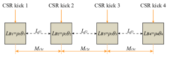
Figure 1: Schematic of a chicane for the two-dimensional point-kick analysis of the CSR effect. The arrows point to the centers of the dipoles. $M_{c1c},M_{c2c}$ and $M_{c3c}$ represent the transfer matrix from the center of dipole 1 to dipole 2, the center of dipole 2 to dipole 3, and the center of dipole 3 to dipole 4, respectively.

Now we calculate the net CSR point-kick. For simplicity, it is assumed that the initial particle coordinates with initial energy deviation $\delta_{0}=0$ in the chicane entrance are $X_{0}=(x_{0},x_{0}^{\prime})^{\dagger}=(0,0)^{\dagger}$. After passing through the section from the center of dipole 1 to the center of dipole 2, the particle experiences the second kick,

$$X_{s2}=M_{c1c,2\times 2}X_{k1}+X_{k2},$$ (9)

Here $C_{1}=\cos(\theta_{1}/2),S_{1}=\sin(\theta_{1}/2)$. From the $2\times 2$ transfer matrix of the horizontal betatron motion in Eqs. (3) and (4), the transfer matrix $M_{c1c,2\times 2}$ between the center of the first two dipoles is given by

$$M_{c1c,2\times 2}=(R_{HB2}R_{d1}R_{HB1})_{2\times 2}=\left[\begin{array}[]{c c}1&L_{d1}+S_{1}\rho_{1}+S_{2}\rho_{2}\\ 0&1\end{array}\right].$$ (10)

Note that Eq. (10) are universal expression for (half dipole)+drift+(half dipole) structure, where one just needs to change the subscripts. Similarly, the particle coordinate deviations after the 4th kick are

$$X_{s4} =M_{c3c,2\times 2}X_{s3}+X_{k4}$$ (11)

$$=M_{c3c,2\times 2}(M_{c2c,2\times 2}X_{s2}+X_{k3})+X_{k4}$$

$$=M_{c3c,2\times 2}M_{c2c,2\times 2}X_{s2}+M_{c3c,2\times 2}X_{k3}+X_{k4}.$$

The description of $M_{c2c,2\times 2}$ and $M_{c3c,2\times 2}$ can be obtained by substituting the $\rho_{1},\rho_{2},S_{1},S_{2},L_{d1}$ in Eq. (10) with the counterparts $\rho_{2},\rho_{3},S_{2},S_{3},L_{d2}$ and $\rho_{3},\rho_{4},S_{3},S_{4},L_{d3}$, respectively. Note that the energy spread $\delta_{j}$ increases by $k_{j}\rho_{j}^{1/3}\theta_{j}$ after passing through the $j$-th dipole, which can be written as

$$\delta_{1}=k_{1}\rho_{1}^{1/3}\theta_{1},~{}~{}~{}\delta_{2}=\sum_{i=1}^{2}k_{i}\rho_{i}^{1/3}\theta_{i},$$ (12)

$$\delta_{3}=\sum_{i=1}^{3}k_{i}\rho_{i}^{1/3}\theta_{i},~{}~{}~{}\delta_{4}=\sum_{i=1}^{4}k_{i}\rho_{i}^{1/3}\theta_{i},$$

respectively. Finally, the particle coordinate deviations $X_{f}$ at the chicane exit are

$$X_{f}=(R_{HB4})_{2\times 2}X_{s4}=\left[\begin{array}[]{c }X_{s4}(1,1)+X_{s4}(2,1)S_{4}\rho_{4}\\ X_{s4}(2,1)\end{array}\right],$$ (13)

where $X_{s4}(1,1),X_{s4}(2,1)$ are the elements of $X_{s4}$ in Eq. (11). Therefore, the CSR-induced emittance growth at the chicane exit can be theoretically cancelled when the particle coordiante deviations satisfy $X_{f}=(0,0)^{\dagger}$ (can also be written as $X_{s4}=(0,0)^{\dagger}$).

Given the considerable complexity of the obtained $X_{z4}$, a Taylor expansion is used to simplify the sine and cosine terms in $X_{z4}$ with respect to the dipole bending $\theta_{i}(i=1,2,3,4)$, where a small bending-angle approximation for the four dipoles is adopted. Besides, we attempt to neglect the lengths of the dipoles as $L_{B}\ll L_{d}$, whereby the two explicit CSR cancelation conditions can be obtained in a greatly simplified form with aid of achromatic condition in Eq. (6) as

$$\frac{q_{2}}{q_{3}q_{4}\ell_{3}}=\frac{\delta_{4}-\delta_{2}}{\delta_{2}},~{}\ell_{2}=-\frac{1}{q_{3}}\frac{q_{3}(\delta_{3}-\delta_{1})+(q_{2}+q_{3})\delta_{2}}{\delta_{2}+(1+q_{2})(\delta_{3}-\delta_{1})},$$ (14)

where $q_{2}=\theta_{2}/\theta_{1},q_{3}=\theta_{3}/\theta_{1},q_{4}=\theta_{4}/\theta_{1},\ell_{2}=L_{d2}/L_{d1},\ell_{3}=L_{d3}/L_{d1}$. Note that Eq. (14) is still complex because the $k_{i}~{}(i=1,2,3,4)$ in Eq. (12) look quite (considerable) tedious (cumbersome).

Next, the important roles of Eq. (14) are revealed. First, Eq. (14) enable us to prove that the symmetric $C$-chicane is impossible to cancel the net CSR point-kick. Combined with these conditions for a symmetric $C$-chicane: $q_{2}=q_{3}=-1,q_{4}=1,\rho_{1}=\rho_{2}=\rho_{3}=\rho_{4}$, and $\ell_{3}=1$, the CSR-cancelation condition in Eq. (14) can be reduced to $k_{1}+k_{2}=k_{3}+k_{4}$. This condition can not be satisfied, because $k_{i}$ in Eq. (8) is almost decreasing with the increasing of $i$ for a compression progress. Second, Eq. (14) also indicates that four is the minimum number of dipoles required to satisfy the CSR-cancelation conditions. This is because, one dipole can cause the CSR effect self-evidently, and a lattice consisting of two different dipoles and a drift will not be achromatic. Importantly, for a chicane with three different dipoles, it can be regarded as a four-bend chicane with one dipole’s bending angle is zero. At this point, the conditions in Eq. (14) can not be satisfied whatever $q_{i}=0~{}(i=2,3,4)$.

One can observe that the seven degrees of freedom (including $q_{2},q_{3},\rho_{2}/\rho_{1},\rho_{3}/\rho_{1},\rho_{4}/\rho_{1},\ell_{2}$ and compression factor $C$ hidden in $k_{i}$), are four more than the number of constraints available (only two conditions as expressed in Eq. (14)). Here the not-mentioned quantities $q_{4},\ell_{3}$ can be obtained from Eq. (6). We do not much care about the value of the $\theta_{1}$ and $L_{d1}$ here, because these are always determined by the design goals, the total length and momentum compaction $R_{56}^{s_{0}\to s_{f}}$ of the chicane.

III An application to four-bend $C$-Chicane

In the following we make the bending angles of the 1st (3rd) dipole and 2nd (4th) dipole identical except for the bending direction, indicating a similarity with the symmetric $C$-chicane. With Eq. (14), we find that to suppress the CSR effect, a “negative drift” between the 2nd and 3rd dipoles is required. Besides the condition $q_{2}=-1$, a chicane with fixed bending radii or fixed dipole lengths is conducted, as introduced in Sec. III.1. Verification of the obtained CSR-cancelation conditions by the integration method and ELEGANT simulations is given in Sec. III.2.

III.1 The CSR-immune $C$-chicane with $\theta_{1}=-\theta_{2}$

Symmetric $C$-chicane is the most widely used bunch compressor type currently. Thus we hope to discuss as much as possible the implementation of a chicane based on a symmetric $C$-chicane. At this point, a condition is added that the first two dipoles have the same bending angle. One can easily obtain that $q_{2}=-1,q_{3}=-q_{4},$ and $\ell_{3}=-1/q_{3}$ from the achromatic condition, while maintaining the parallelism of the beam orbits between the 2nd and 3rd dipoles. The schematic figure is shown in Fig. 2. This condition greatly simplifies the structure of the chicane, as the four different dipoles are now reduced to two types of dipole. And the bending angle ratio $q_{3}$ is an obvious sign to understand the CSR compensation later.

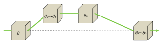
Figure 2: General geometry of an asymmetric $C$-chicane. The space between the 2nd and 3rd dipoles is parallel to the entrance or exit of the beam, which is a “negative drift” constructed by several quadrupoles.

Based on the constraints $q_{2}=-1,q_{3}=-q_{4},$ and $\ell_{3}=-1/q_{3}$ given above, the CSR-cancelation conditions in Eq. (14) can be reduced to

$$-\frac{1}{q_{3}}=\frac{\delta_{4}-\delta_{2}}{\delta_{2}},~{}~{}\ell_{2}=-\frac{q_{3}(\delta_{3}-\delta_{1})+(q_{2}+q_{3})\delta_{2}}{q_{3}\delta_{2}}.$$ (15)

It turns out that $\ell_{2}=L_{d2}/L_{d1}$ is negative because $q_{2}$ and $q_{3}$ have the same sign and $\delta_{3}-\delta_{1},\delta_{2}$ remain positve. And the “negative drift” can be regarded as a focus section achieved by several quadrupoles and drifts cite:Chao . Despite the presence of “negative drift”, note that the dispersion and the beam trajectory are not affected, since the trajectory is independent of $L_{d2}$ under the condition of $\theta_{1}=-\theta_{2}$ (see Eqs. (5) and (6)). In this section we use $L_{d2}^{\text{real}}(\ell_{2}^{\text{real}})$ to describe the real length of the physical space, and $L_{d2}^{\text{eff.}}(\ell_{2}^{\text{eff.}})$ for a focus section whose transfer matrix is a “negative drift”.

In order to put our theoretical calculation into practice, two typical cases are discussed to elaborate the CSR-cancelation conditions in Eq. (15). Case 1 is a chicane where the four dipoles have the same bending radii and case 2 is a chicane with fixed dipole lengths. These two cases typically correspond to the following two scenarios: For the dipole design phase, priority is given to case 1, where the bending radii are fixed by setting the same magnetic field $B_{0}$. Case 2 is typically used for pre-manufactured dipoles, allowing for adjustment of the dipole’s bending angle by changing $B_{0}$.

For case 1, bending radii are fixed value as $|\rho_{1}|=|\rho_{2}|=|\rho_{3}|=|\rho_{4}|$. The difference between the first two dipoles and the last two dipoles is mainly reflected by the angles retio $q_{3}=\theta_{3}/\theta_{1}$. The parameters $k_{i}~{}(i=1,2,3,4)$ in Eq. (15) satisfy $k_{i}\propto(1+h~{}R_{56}^{s_{0}\to s_{i}})^{-4/3}$ with a $C$-relevant linear momentum chirp $h$, as presented in Appendix A. Thus CSR-cancelation conditions can be written as

$$C^{-4/3}+(\frac{2(1-q_{3})}{1+C-2Cq_{3}})^{4/3}=q_{3}^{2}\left(1+(\frac{2(1-q_{3})}{2-q_{3}-Cq_{3}})^{4/3}\right),$$ (16)

and

$$\ell_{2}^{\text{eff.}}= -1+\frac{1}{q_{3}}-\frac{(2C(1-q_{3}))^{4/3}}{(C-2Cq_{3}+1)^{4/3}+(2C(1-q_{3}))^{4/3}}$$ (17)

$$+\frac{2^{4/3}}{q_{3}((\frac{2-(1+C)q_{3}}{1-q_{3}})^{4/3}+2^{4/3})}.$$

Note that the bending angle ratio $q_{3}$ depends only on the compression factor $C$, and is independent of the value of $\ell_{2}^{\text{eff.}}$. As shown in Fig. 3, the solved $q_{3}$ is equal to $-1$ when the bunch compressed by a factor of $C=1$ (no compression), then the value of $|q_{3}|$ becoming smaller as the factor $C$ increases. For approximation, Eq. (16) can be written as a simpler expression as $q_{3}\approx-C^{-1/2}$ for factor $C<25$. The comparison between the approximate and theoretical results is shown in Fig. 3 by the solid and dashed curves. Equation (16) also indicates that the weaker last two dipoles suppress CSR effects better, which is reasonable because the bunch length is shortest at the last two dipoles, where CSR is strongest Borland:2001xv . It is worth noting that this conclusion is consistent with the parameter scan results of the CSRTRACK simulations in Stulle:2007se .

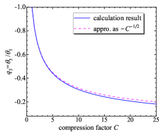
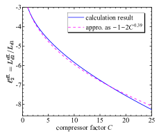
Figure 3: The required bending angle ratio $q_{3}=\theta_{3}/\theta_{1}$ (top) and ratio $\ell_{2}^{\text{eff.}}=L_{d2}^{\text{eff.}}/L_{d1}$ (bottom) vary with the compression factor $C$ from CSR-cancelation conditions Eqs. (16) and (17) (solid blue curve) under case 1. The dashed pink curves show simpler expression $q_{3}\approx-C^{-1/2}$ and $\ell_{2}^{\text{eff.}}\approx-1-2C^{0.39}$, respectively.

Substituting the $q_{3}$ (Eq. (16)) in Eq. (17), we calculate the value of $\ell_{2}^{\text{eff.}}$, as a function of the compression factor $C$, as shown in Fig. 3. We find that with Eq. (17), $\ell_{2}^{\text{eff.}}$ equals $-3$ when the factor is $C=1$. It is concluded that the quantities ($q_{3},\ell_{2}^{\text{eff.}}$) can be qualitatively approximated by simpler expressions,

$$q_{3}=-C^{-1/2},~{}~{}~{}\ell_{2}^{\text{eff.}}=-1-2C^{0.39},$$ (18)

for the case of fixed bending radii.

For case 2, the bending lengths satisfy $L_{B1}=L_{B2}=L_{B3}=L_{B4}$. Similarly to case 1, we obtain the empirical equations of $q_{3}$ and $\ell_{2}^{\text{eff.}}$ for the factor $C<25$ as

$$q_{3}\approx-C^{-3/5},~{}~{}~{}\ell_{2}^{\text{eff.}}\approx-1-2C^{0.47}.$$ (19)

From Eqs. (18) and (19), it can be seen that the bending radii of the last two dipoles in case 2 are weaker than in case 1, and a larger $|\ell_{2}^{\text{eff.}}|$ is needed to suppress the CSR effect in this case.

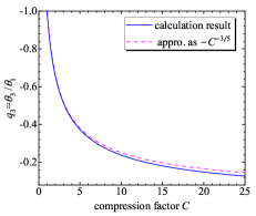
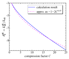
Figure 4: The required bending angle ratio $q_{3}=\theta_{3}/\theta_{1}$ (top) and ratio $\ell_{2}^{\text{eff.}}=L_{d2}^{\text{eff.}}/L_{d1}$ (bottom) vary with the compression factor $C$ from CSR-cancelation conditions under case 2 (solid blue curve). The dashed pink curves show simpler expression $q_{3}\approx-C^{-3/5}$ and $\ell_{2}^{\text{eff.}}\approx-1-2C^{0.47}$, respectively.

Finally, the chicane design goal, the momentum compaction $R_{56}^{s_{0}\to s_{f}}$ and total length $L_{tot}$, can be obtained from the value of $L_{d1}$, $\theta_{1}$, and the provided $q_{3}$ as

$$R_{56}^{s_{0}\to s_{f}}=-L_{d1}\theta_{1}^{2}(1-q_{3}),~{}~{}L_{tot}=\ell_{2}^{\text{real}}+L_{d1}(1-1/q_{3}).$$ (20)

It indicates that for a fixed design target and a larger bending angle ratio $|q_{3}|$, there will roughly be a smaller $L_{d1}$ and a larger $\theta_{1}$ and vice versa. In this way the comparison of different chicanes with the same design goal becomes easier.

In principle, the proposed design has the same overall structure as the symmetric $C$-chicane except (i) the deflection magnitude of the last two dipoles is weaker than the first two with a ratio of $q_{3}=\theta_{3}/\theta_{1}$. (ii) the distance between the 3rd and 4th bends is increased until the ratio $\ell_{3}=-1/q_{3}$ is satisfied. (iii) a focus section with a physical length $L_{d2}^{\text{real}}$ is provided between the 2nd and 3rd dipoles, consisting of several quadrupoles.

III.2 Numerical verification of the proposed conditions

In the above sections, generic and explicit CSR cancelation conditions have been obtained for an asymmetric $C$-chicane. However, these conditions in Eq. (15) are derived with some assumptions: the bunch length variation in a single dipole is not considered and the length of the dipoles is neglected. Therefore, one of the main purposes of this subsection is to investigate the $(q_{3},\ell_{2}^{\text{eff.}})$ that satisfies the CSR-cancelation conditions included these assumptions, and then to compare it with the result from the point-kick model. Both numerical integration method and ELEGANT particle tracking simulations are presented. In the presence of these two methods, however it is almost impossible to achieve an analytical solution for compression progress.

To this end, the dipole lengths are further taken into account. With aid of the Eq. (5), the drift length $L_{d3}$, the momentum compaction $R_{56}^{s_{0}\to s_{f}}$, and total length $L_{tot}$ in Eq. (20) can be exported by more complex expressions (see Appendix B). Next a numerical chicane design goal need to be specied. We set a design goal based on a symmetric $C$-chicane with typical parameters of equal dipole length of 0.5 m, bending angle of 3^∘, the compression goal of $C=10$, the 1st and 3rd drift lengths of $6.5\text{ m}$, and the 2nd drift length of 5 m. Thus the complete information for such $C$-chicane can be obtained, as listed in Tables 1 and 2. For the convenience of comparison, the acquired $L_{tot}$, $R_{56}^{s_{0}\to s_{f}}$, tegother with the 1st dipole length and compression factor (Table 1), are common to all chicanes compared in this paper.

For illustration, the CSR-induced coordinate deviations are evaluated by a semi-classical numerical analysis using a numerical integration method Emma:1997hj , which allows for the bunch length variation within each dipole. Hence the bunch parameters $k_{1},k_{2},k_{3},k_{4}$ in Eq. (12) are no longer set to a fixed value for each dipole, but are modified as follows

$$k_{i}=k_{0}(1+h~{}R_{56}^{s_{0}\to s})^{-4/3},~{}~{}(i=1,2,3,4)$$ (21)

where $R_{56}^{s_{0}\to s}$ in different positions, as a function of $\phi$, are expressed in Appendix C. Here $\phi$ and the subscript “$s$” are the angle and position that the beam traverses in a dipole magnet, respectively. Thus the CSR-cancelation conditions for a chicane can be evaluated using an integration method as Emma:1997hj

$$\Delta x_{f}^{2}=\left[\sum_{i=1}^{4}\rho_{i}^{1/3}\int_{B}k_{i}~{}R_{16}^{s\rightarrow s_{f}}d\phi\right]^{2}=0,$$ (22)

$$\Delta x_{f}^{\prime 2}=\left[\sum_{i=1}^{4}\rho_{i}^{1/3}\int_{B}k_{i}~{}R_{26}^{s\rightarrow s_{f}}d\phi\right]^{2}=0,$$

here both $R_{16}^{s\rightarrow s_{f}}$ and $R_{26}^{s\rightarrow s_{f}}$ vary as a function of $\phi$ in dipoles (see Appendix C for details).

Table 1: Parameters common to all bunch compressor chicanes compared in this paper.

	Symbol	chicane Parameters	Unit
Total length	$L_{tot}$	20	m
first-order momentum	$R_{56}^{s_{0}\to s_{f}}$	37.5	mm
compaction
Compression factor	$C$	10	—
Length of the 1st dipole	$L_{B1}$	0.50	m

Table 2: Parameters of the symmetric and asymmetric $C$-chicane settings under case 1 with unit m.

	Symbol	symmetric	asymmetric
		$C$-chicane	$C$-chicane
Length of the first two dipoles	$L_{B1},L_{B2}$	0.50	0.50
Length of the last two dipoles	$L_{B3},L_{B4}$	0.50	0.14
Bending radii of each dipole	$\rho$	9.55	4.99
Length of the 1st drift	$L_{d1}$	6.5	2.57
Length of the 3rd drift	$L_{d3}$	6.5	11.16
effective value of the 2rd drift	$L_{d2}^{\text{eff.}}$	—	-20.05

To verify the theoretical value (Eqs. (16) and (17)) of $q_{3}^{*}=-0.30,\ell_{2}^{\text{eff.}*}=-5.84$ for case 1 for a bunch compressed by a factor of 10, some chicane parameters need to be specified for the integration calculation. Here we consider a case with equal disign goal (listed in Table 1), and a physical length of $L_{d2}^{\text{real}}=5\text{ m}$. From the integration method, the calculation results of $(\ell_{2}^{\text{eff.}}/\ell_{2}^{\text{eff.}*},q_{3}/q_{3}^{*})=(1.358,0.894)$ can be derived from $|\Delta x_{f}|=0$ m and $|\Delta x_{f}^{\prime}|=0$, as shown in the pink pentacle in Fig. 5. Here $\ell_{2}^{\text{eff.}}$ and $q_{3}$ are normalized with respect to $\ell_{2}^{\text{eff.}*}$ and $q_{3}^{*}$ just for clear comparison. It shows that the agreement between the analytical and numerical calculations is basically good.

Astonishingly, we notice an apparent independence of the value of $q_{3}$ with $\ell_{2}^{\text{eff.}}$, as shown by the red curve in Fig. 5. This independence can be attributed to the fact that $L_{d2}^{\text{eff.}}$ vanishes during the integration. From this perspective, the CSR-cancelation condition $\Delta x_{f}^{\prime}=0$ can be achieved simply by adjusting the dipoles.

On the other hand, to verify the proposed CSR-cancelation conditions, the emittance growth caused by dipole-induced CSR after passing through the chicane is simulated with the ELEGANT program Borland:2000gvh ; Borland:2001xua . The Gaussian bunch with typical initial parameters is tracked as listed in Table 3. The beam optical elements are second order, and the momentum chirp is set as $h=(1-C)/(CR_{56}^{s_{0}\to s_{f}})=24.02$ m^-1 from the compressor factor and $R_{56}^{s_{0}\to s_{f}}$ in Table 1. By scanning $(\ell_{2},q_{3})$ and the initial Twiss parameters, we are committed to achieving minimum emittance growth at the chicane exit. Such Twiss parameter scanning is performed to search for an optimal matching beam envelope to the orientation of a nonzero net CSR kick for a practical chicane DiMitri:2013qj . As shown in Fig. 6, we can see that the scanned values $(\ell_{2}^{\text{eff.}}/\ell_{2}^{\text{eff.}*},q_{3}/q_{3}^{*}$)=(1.38, 0.91) are basically close the results of the point-kick model and the CSR-induced $\Delta\varepsilon_{n}/\varepsilon_{n}$ at the order of 0.1%. With aid of the common chicane parameters in Table 1, the complete chicane information for this case are listed in Table 2.

Table 3: The initial and final beam parameters for the ELEGANT simulations.

beam Parameters	Symbol	Value	Unit
Bunch charge	$Q$	300	pC
Initial rms bunch length	$\sigma_{zi}$	100	$\mu$m
Final rms bunch length	$\sigma_{zf}$	10	$\mu$m
Beam energy	$E_{0}$	3	GeV
Norm. emittance	$\varepsilon_{n0}$	0.9	$\mu$m.rad
Uncorr. energy spread	$\sigma_{\delta}$	0.002	%

In the above numerical verification by integration method and ELEGANT simulations, the differences compared to the model calculation, can be attributed to the ratio between $L_{B1}$ and ($L_{tot}-L_{d2}^{\text{real}}$). With this ratio decreases, $(\ell_{2}^{\text{eff.}},q_{3})$ becomes closer to $(\ell_{2}^{\text{eff.}*},q_{3}^{*})$, as illustrated in Fig. 5. Although some fine-tuning is still required compared to the model calculation, these differences are minor and can be compensated for in the actual design process by minor parameter adjustments. Notice that the integration and simulations methods can yield more accurate results, however the point-kick model directly provides analytical relationships between variables to suppress the CSR effect albeit with slight differences.

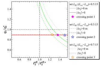
Figure 5: The $(\ell_{2}^{\text{eff.}}/\ell_{2}^{\text{eff.}*},q_{3}/q_{3}^{*}$) of a $C=10$ chicane with $|\Delta x_{f}|=0$ m and $|\Delta x_{f}^{\prime}|=0$, as shown in the solid green and red curves. The pink pentacle is the crossing point of the two curves. As a comparison, the results for $L_{B1}$:$(L_{tot}-L_{d2}^{\text{real}})=$0.3:15, 0.5:15 and 0.7:15, are calculated as $(\ell_{2}^{\text{eff.}}/\ell_{2}^{\text{eff.}*},q_{3}/q_{3}^{*}$)=(1.246, 0.899), (1.358, 0.894) and (1.494, 0.889), respectively.

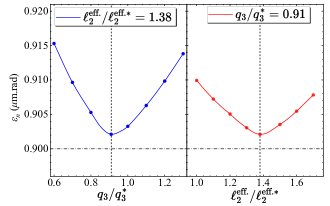
Figure 6: The ELEGANT simulations result of the CSR-induced emittance $\varepsilon_{n}$ near $(q_{3}^{*},\ell_{2}^{\text{eff.}*})$ for $C=10$ asymmetric $C$-chicane, and it turns out that the parameters satisfy $(q_{3}/q_{3}^{*},\ell_{2}^{\text{eff.}}/\ell_{2}^{\text{eff.}*})=(0.91,1.38)$, as shown in the dashed curves.

IV An application to four-bend $S$-Chicane

While the $S$-chicanes are rarely used in FELs compared to the $C$-chicanes, the existing works reveal that the $S$-like chicanes seem to easily preserve the CSR-induced emittance Antipov:2021eko ; Stulle:2007se ; Beutner:2007zza ; Khan:2022tkg , of course, five or six dipoles are needed in such $S$-like chicanes. In this section we demonstrate a more ambitious idea of achieving a CSR-eliminated four-bend chicane without focus section between adjacent dipoles. It turns out that such chicane must be a $S$-chicane, as proved in Sec. IV.1, and four dipoles are sufficient to achieve a CSR-eliminated chicane. To fulfil such chicane design requirement, additional conditions are necessary. Apart from the position condition $L_{d1}/L_{tot}=1/4$, a chicane with fixed bending radii or fixed dipole length are added, as introduced in Sec. IV.2. The verification of the CSR-cancelation conditions by the integration method and numerical tracking by ELEGANT are given in Secs. IV.3.

IV.1 The positive drift conditions for four-bend chicane

Substituting the achromatic condition in Eq. (14), one can obtain the drift lengths ratio of $L_{d2}/L_{d1}$ and $L_{d3}/L_{d1}$ as

$$\ell_{2}= -\frac{1}{q_{3}}\frac{q_{3}(\delta_{3}-\delta_{1})+(q_{2}+q_{3})\delta_{2}}{\delta_{2}+(1+q_{2})(\delta_{3}-\delta_{1})},$$ (23)

$$\ell_{3}= \frac{1}{q_{3}}\frac{q_{2}\delta_{2}}{\delta_{2}+(1+q_{2})(\delta_{3}-\delta_{1})}.$$

Our aim is to get both $\ell_{2}$ and $\ell_{3}$ positive. Noticeably, $\delta_{3}-\delta_{1}$ and $\delta_{2}$ remain positive, and the signs of $q_{2}$ and $q_{3}$ are unknown, thus they can be classified into four groups:

1. set $q_{2}>0$ and $q_{3}>0$. This group is not applicable becuse $\ell_{2}<0$.

2. set $q_{2}>0$ and $q_{3}<0$. This group is not applicable becuse $\ell_{3}<0$.

3. set $q_{2}<0$ and $q_{3}<0$. As $\ell_{3}>0$, one can obtain $\delta_{2}+(1+q_{2})(\delta_{3}-\delta_{1})>0$. Thus $q_{3}(\delta_{3}-\delta_{1})+(q_{2}+q_{3})\delta_{2}>0$ as $\ell_{2}>0$. However, $q_{3}(\delta_{3}-\delta_{1})+(q_{2}+q_{3})\delta_{2}>0$ is impossible as $q_{2}<0,q_{3}<0$.

4. set $q_{2}<0$ and $q_{3}>0$. Both $\ell_{2}>0$ and $\ell_{3}>0$ is possible under the condition that $q_{3}(\delta_{3}-\delta_{1})+(q_{2}+q_{3})\delta_{2}>0$ and $\delta_{2}+(1+q_{2})(\delta_{3}-\delta_{1})<0$. Thus the result $1+q_{2}<0$ can be achieved.

The sign of $q_{4}$ can be specified from Eq. (14), and it turns out to be a negative $q_{4}$. Another advantage is that the negative $q_{4}$ can ensure a shorter and shorter bunch length and an increasing $|R_{56}^{s_{0}\to s}|$ after crossing each dipole (see Appenidx A).

To sum up, a chicane with three positive drifts must satisfy

$$q_{2}<0,~{}q_{3}>0,~{}q_{4}<0,~{}1+q_{2}<0,~{}\frac{\delta_{3}-\delta_{1}}{\delta_{2}}>-\frac{1}{1+q_{2}}.$$ (24)

One can find that this is a $S$-chicane (Fig. 7) from the angle relation. The last condition in Eq. (24) is easily realizable, which can be achieved by adjusting the bending radii $\rho_{i}(i=1,2,3)$ in $\delta_{3}-\delta_{1}$ and $\delta_{2}$.

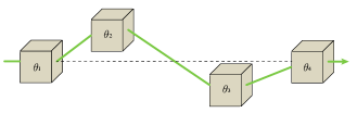
Figure 7: General geometry of an asymmetric $S$-chicane. The drift length between the 1st and 2nd dipoles is a quarter of the chicane total length.

IV.2 the CSR-immune $S$-chicane with $L_{d1}/L_{tot}=1/4$

We define the symmetric $S$-chicane as one in which the dipoles 1 and 4 have equal bending strength and the dipoles 2 and 3 are of double that, otherwise it is called asymmetric. Note that the symmetric $S$-chicane satisfies the position conditions that $2L_{d1}=L_{d2}=2L_{d3}$. In this subsection, we discuss the implementation of a chicane based as much as possible on the symmetric $S$-chicane, while comparing the symmetric and asymmetric $S$-chicane as a reference for our discussion.

Two typical cases are discussed in this subsection. Similar to Sec. III, case 1 and case 2 are a chicane with the four dipoles having fixed bending radii or fixed dipole lengths, respectively. Nevertheless, the four independent variables $q_{2},q_{3},\ell_{2}$, and $C$ cannot be solved from the two CSR cancelation conditions, unless a constraint is added to eliminate a free quantity. To mimic the structure of a symmetric $S$-chicane, the ratio $L_{d1}/L_{tot}=1/4$ is set as we intend to adjust fewer dipoles and more bending angles, when the total length constant. At this point, the longitudinal positions of dipoles 1, 2 and 4 are fixed. Combined with the achromatic condition in Eq. (6), the variables $q_{4}=\theta_{4}/\theta_{1},\ell_{2}=L_{d2}/L_{d1},\ell_{3}=L_{d3}/L_{d1}$ can be expressed with $q_{2},q_{3}$ as

$$q_{4}=-(1+q_{2}+q_{3}),~{}~{}\ell_{2}=\frac{4}{q_{3}}+3(\frac{q_{2}}{q_{3}}+1),~{}~{}\ell_{3}=-\frac{4}{q_{3}}-\frac{3q_{2}}{q_{3}}.$$ (25)

Despite fixing the 2nd dipole is not the only option with additional conditions, it is more operational to change the bending angles of the four dipoles, than to move the position one.

For case 1, the bending radii are set to $\rho_{1}=-\rho_{2}=\rho_{3}=-\rho_{4}$. The relations between $k_{1},k_{2},k_{3},k_{4}$ in Eq. (14) are calculated in Appendix A. As the overcomplicated equations in Eq. (14), we solve the numerical solutions of $q_{2}$ and $q_{3}$ as a function of the factor $C$, as shown in Fig. 8. This result can be checked by solving Eqs. (14), (25) under case 1. Based on the obtained $q_{2}$ and $q_{3}$, the value of $q_{4},\ell_{2},\ell_{3}$ in Eq. (25) are shown in Figs. 8 and 9, which is varies only with factor $C$.

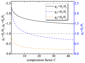
Figure 8: The solved $q_{2}=\theta_{2}/\theta_{1},q_{3}=\theta_{3}/\theta_{1}$ from Eqs. (14), (25) as a function of compression factor $C$ under case 1. The corresponding $q_{4}=\theta_{4}/\theta_{1}$ are also included.

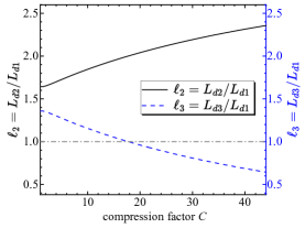
Figure 9: The corresponding $\ell_{2}=L_{d2}/L_{d1},\ell_{3}=L_{d3}/L_{d1}$ after solving the $q_{2}=\theta_{2}/\theta_{1},$ and $q_{3}=\theta_{3}/\theta_{1}$ under case 1.

For case 2, the dipole lengths are fixed as $L_{B1}=L_{B2}=L_{B3}=L_{B4}$. So the bending radii ratios $\rho_{2}/\rho_{1}=1/q_{2}$, $\rho_{3}/\rho_{1}=1/q_{3}$, $\rho_{4}/\rho_{1}=-1/(1+q_{2}+q_{3})$ can be derived. In a similar manner to case 1, the value of $q_{2}=\theta_{2}/\theta_{1},q_{3}=\theta_{3}/\theta_{1}$ can be solved from Eqs. (14), (25). We find that the absolute value of $q_{2},q_{3}$ in case 2 (see Fig. 10) shows high similarity to case 1. Correspondingly, the $q_{4},\ell_{2},\ell_{3}$ under case 2 are plotted in Figs. 10 and 11.

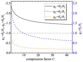
Figure 10: The solved $q_{2}$ and $q_{3}$ as a function of compression factor $C$ under case 2. The corresponding $q_{4}=\theta_{4}/\theta_{1}$ are also included.

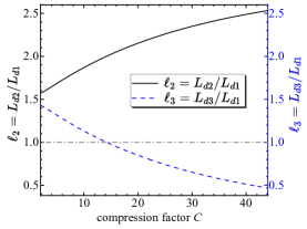
Figure 11: The corresponding $\ell_{2}$ and $\ell_{3}$ after solving the $q_{2}$ and $q_{3}$ under case 2.

We find that, the theoretical results in both case 1 and case 2 show that the last two dipoles are weaker than the first two dipoles for a symmetric $S$-chicane. More specifically, the dipole 3(4) is weaker than the dipole 2(1) for both case 1 and case 2, as shown in Figs. 8 and 10. This weakening becomes more pronounced as the compression factor increases.

We also find that a symmetric $S$-chicane cannot satisfy the CSR-cancelation conditions in our calculation, since no compression factor $C$ in Figs. 8 and 10 satisfies both $q_{2}=-2$ and $q_{3}=2$. Then an interesting question arises, whether a CSR-cancelled chiacne can be achieved, by fine adjustments of a symmetric $S$-chicane with four equal-length dipoles and fixed dipole positions. To this end, just adjust the strength of the dipoles to $q_{2}=-1.62,q_{3}=0.87,q_{4}=-0.25$ according to Fig. 10 (or Eq. (14)). Because the compression factor $C$ is equal to $14.2$ in case 2 when $L_{d2}/L_{d1}=2,L_{d3}/L_{d1}=1$ is satisfied from Fig. 11. Finally, the asymmetric $S$-chicane with cancelled CSR is activated. Of course, the subtleties of the theory cannot always be fully demonstrated in the experiment. Therefore, further simulations and even experimental verification will be essential.

IV.3 Numerical verification of the proposed conditions

A numerical analysis is provided to verify the CSR-cancelation conditions for asymmetric $S$-chicane with specific chicane parameter settings in Table 1. First, the dipole lengths are taken into account. The expressions of $\ell_{2},\ell_{3}$ in Eq. (23) and the value of $R_{56}^{s_{0}\to s_{f}}$, $L_{tot}$ are recalculated, the details of which can be found in Appendix B. Second, the bunch length variation can be considered in a similar manner to the asymmetric $C$-chicane using an integration method Emma:1997hj . These variables $R_{16}^{s\rightarrow s_{f}}$ and $R_{26}^{s\rightarrow s_{f}}$ in Eq. (22), and $R_{56}^{s_{0}\to s}$ in $k_{1},k_{2},k_{3},k_{4}$, are changing with the position $s$, as expressed in Appendix C. Finally, the obtained CSR cancelation conditions $(q_{2},q_{3})$ can be obtained and compared with the results $q_{2}^{*}=-1.75$, $q_{3}^{*}=1.09$ (Eq. (14)) for case 1 when the compression factor is $C=10$. The integration results $(q_{2}/q_{2}^{*},q_{3}/q_{3}^{*})=(0.954,0.883)$ (shown in Fig. 12), indicates a relatively accurate calculation of the point-kick model. Similar to the $C$-chicane, the $(q_{2},q_{3})$ obtained by integration method, can be closer to the result of the point-kick model after reducing the ratio $L_{B1}:L_{tot}$, as shown in Fig. 12. In fact, model calculation trade this slight loss of accuracy for more general CSR cancelation.

Furthermore, the minimum transverse emittance $\varepsilon_{n}$ for the asymmetric $S$-chicane, together with the corresponding $(q_{2},q_{3})$, is searched by ELEGANT simulations. The scaned results $(q_{2}/q_{2}^{*},q_{3}/q_{3}^{*})=(0.95,0.88)$ are obtained, and this result close to (1,1) indicates a accurate calculation by the point-kick model. For illustration, the variation of the growth in normalized emittance near $(q_{2}/q_{2}^{*},q_{3}/q_{3}^{*})$ are displayed in Fig. 13. The complete asymmetric $S$-chicane information can be found in Table 4.

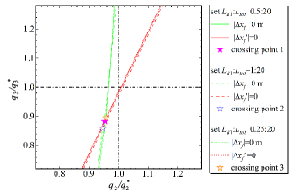
Figure 12: The ($q_{2}/q_{2}^{*},q_{3}/q_{3}^{*}$) of a $C=10$ chicane with $|\Delta x_{f}|=0$ m and $|\Delta x_{f}^{\prime}|=0$, as shown in the solid green and red curves. As a comparison, the result for $L_{B1}:L_{d1}$=0.25:20, 0.5:20 and 1:20 are calculated as $(q_{2}/q_{2}^{*},q_{3}/q_{3}^{*})=$ (0.958, 0.895), (0.954, 0.883), and (0.947, 0.859), respectively.

Table 4: Parameters of the symmetric and asymmetric $S$-chicane settings under case 1 with unit m.

	Symbol	symmetric	asymmetric
		$S$-chicane	$S$-chicane
Bending radii of each dipole	$\rho$	10.96	7.12
Length of the 2nd dipole	$L_{B2}$	1	0.84
Length of the 3rd dipole	$L_{B3}$	1	0.48
Length of the 4th dipole	$L_{B4}$	0.5	0.14
Length of the 1st drift	$L_{d1}$	4.125	4.08
Length of the 2nd drift	$L_{d2}$	8.75	8.78
Length of the 3rd drift	$L_{d3}$	4.125	5.18

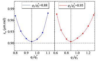
Figure 13: The ELEGANT simulations result of the CSR-induced emittance $\varepsilon_{n}$ near $(q_{2},q_{3})$ for $C=10$ asymmetric $S$-chicane, and it turns out that the parameters satisfy $(q_{2}/q_{2}^{*},q_{3}/q_{3}^{*})=(0.95,0.88)$.

V comparation among symmetric and asymmetric $C$- and $S$-chicanes

In this section, to further demonstrate the CSR suppression efficiency of our proposed chicane designs, we compare the performance in suppressing the CSR-induced emittance growth between symmetric and asymmetric $C$- and $S$-chicanes, which have the same $L_{tot}$, $R_{56}^{s_{0}\to s_{f}}$, $L_{B1}$, and compression factor $C$, as summarized in Table 1. The other chicane parameters are presented in Tables 2 and 4. These chicanes are tested by ELEGANT with the initial bunch parameters in Table 3.

For the cases with CSR-induced emittance growth, by scanning the initial C-S parameters, we are committed to achieving minimum emittance growth in the exit of the symmetric $C$- and $S$-chicanes. By doing so, the ELEGANT simulations results are summarized in Table 5. In the case of the asymmetric $C$- and $S$-chicanes, the growth in normalized emittance $\Delta\varepsilon_{n}/\varepsilon_{n0}$ are reduced by tenfold compared to the symmetric ones, It appears that the emittance growth due to CSR can be well suppressed. In addition, some studies have shown that a longer drift space between the dipoles degrades the emittance, as the CSR effects dominate in the drift space Borland:2001xv . Therefore, it is necessary to investigate the CSR suppression efficiency under a more detail case, considering the incoherent synchrotron radiation (ISR) in the bending magnets, and the CSR effect in the dipoles and the following drift space with the Stupakov model Borland:2000gvh . It shows that the relative emittance growth of symmetric $C$- and $S$-chicanes (Table 5) are 4.5 and 10 times larger than that of asymmetric ones, respectively. These results appear good suppression of the emittance growth, whether only the dipole-induced CSR or the full effect is considered.

Note that the increase in emittance is mainly due to the CSR effects in the drift space after this dipole, which is consistent with the conclusions in Borland:2000gvh . Therefore, it is essential to investigate the CSR suppression efficiency using a more detailed physical model of the CSR wake in order to reduce this effect by appropriately deviating from the current result.

Table 5: Results of the ELEGANT simulations of the finally geometric emittance $\varepsilon_{nf}$, and relative emittance growth $\Delta\varepsilon_{n}/\varepsilon_{n0}$ for symmetric and asymmetric $C$- and $S$-chicane with initial emittance $\varepsilon_{n0}=0.9\text{ mm.rad}$.

CSR effects	$\varepsilon_{nf}$ (mm.rad)	$\Delta\varepsilon_{n}/\varepsilon_{n0}$
asymmetric $C$-chicane
CSR-induced only	0.9021	$2.3\times 10^{-3}$
all effect	1.0628	0.181
symmetric $C$-chicane
CSR-induced only	1.0745	0.194
all effect	1.6398	0.822
asymmetric $S$-chicane
CSR-induced only	0.9041W	$4.9\times 10^{-3}$
all effect	0.9376	0.042
symmetric $S$-chicane
CSR-induced only	1.0115	0.124
all effect	1.2871	0.430

VI Summary

This paper reports theoretical designs for asymmetric $C$- and $S$-chicanes bunch compressors, both of which can suppress the CSR-induced transverse emittances during bunch compression. The design of the asymmetric $C$-chicane may be valuable for improving on the current numerous asymmetric $C$-chicanes. And the asymmetric $S$-chicane will be advantageous for future bunch compressors. The theoretical CSR-cancelation conditions for two chicanes with four different dipoles are derived using a point-kick model. For the asymmetric $C$-chicane, the ratio $q_{3}=\theta_{3}/\theta_{1}=-L_{d1}/L_{d3}$ is required to adjust the bending angle ratio between the first two dipoles and the last two, and the drift ratio between the first drift and the third. Despite a “negative drift” between the 2nd and 3rd dipoles, such a $C$-chicane is realizable by adding quadruples. Correspondingly, the ratio $q_{3}$ and the effective value of the “negative drift” can be approximated to be a simpler expression as Eqs. (18) and (19). For the asymmetric $S$-chicane, the value of $(\theta_{2}/\theta_{1},\theta_{3}/\theta_{1})$ can be solved by solving equations, including the position condition in Eq. (25), and the CSR cancelation conditions in Eq. (14) for the cases of fixed bending radii and fixed dipole lengths, respectively. Roughly, both the values of $(\theta_{3}/\theta_{1},L_{d2}^{\text{eff.}}/L_{d1})$ for $C$-chicane and $(\theta_{2}/\theta_{1},\theta_{3}/\theta_{1})$ for $S$-chicane can be determined as compression factor $C$-dependent quantities, which is applicable to arbitrary chicane design goal. As a verification of these theoretical results, numerical integration calculations and ELEGANT simulations for asymmetric $C$- and $S$-chicanes are presented, which show a slight shift with respect to the theoretical result. Compared to the symmetric $C$- and $S$-chicanes with the same compression target, the asymmetric ones show a promising performance in suppressing the emittance growth in our simulations.

One can find that the key to supressing the CSR effect is to weaken the strength of the last two dipoles according to certain rules, whether for $C$- or $S$-chicane. This feature coinsides with the asymmetric DBA-based bunch compressor introduced in Zhang:2023cgl , where the 2nd dipole is $C^{-1/3}$ or $C^{-1/2}$ times weaker than dipole 1. An intriguing pattern emerges that the asymmetric $C$- and $S$-chicane, as well as the DBA-based bunch compressor are homologous and delicately governs the CSR of the bunch during the compression process.

While the primary focus of this paper lies in analyzing the design principles that effectively suppress CSR-induced emittance growth in the chicane bunch compressors, we also assess the potential microbunching instability associated with the lattice and the beam parameters. Using our developed semi-analytical Vlasov solver Tsai:2017hef ; Tsai:2020ddc enables the fast, efficient evaluation of the various lattice designs. The semi-analytical calculations indicate that these chicane designs, which are effective in suppressing CSR-induced emittance growth, also exhibit a well-controlled microbunching instability. Specifically, based on the beam parameters and chicane settings presented in Tables 1, 2, and 3, taking into account both the steady-state and transient CSR and the longitudinal space charge (LSC) effects, the simulation results for the C-chicane reveal a maximum gain of about 3.5 occurring around an initial modulation wavelength of 50 $\mu$m. In the case of the $S$-chicane, simulation results demonstrate a maximum gain of 4 around a similar modulation wavelength of 50 $\mu$m. In addition, other collective effects, such as space-charge forces, beam-beam effects, and many others, are not considered in this paper. In a practical accelarator, these are difficult to cancel out and need to be fully taken into account.

We hope that our results can be used as a starting point for CSR-cancelled chicane bunch compression and can be verified experimentally. A feasible verification scheme based on the current symmetric $C$-chicane is, to insert a “negative drift” section between the 2nd and 3rd dipoles, and to increase the strength of the first two dipoles and decrease the last two, while adjusting the longitudinal position of the 2nd and 3rd dipoles. The usability of confirming the design of the asymmetric $S$-chicane is more feasible. Based on a symmetric $S$-chicane, try to move the position of the 3rd dipole and vary the current of the dipoles to control their bending strength. Becides, based on the current numerous $C$-chicanes, changing the positive and negative poles of the last two dipole currents seems to be a convenient approach. This paper opens up new avenues for the realisation of CSR-supressed bunch compressor, and it is hoped that this design will provide guidance on the future development of chicane based scientific facilities and applications.

Appendix A $k_{i}$ for different dipoles

Here we assume that the bunch length is constant in a single dipole for point-kick model, so each magnet corresponds to a constant $k_{i}$. Concretely, the $k_{1}$ for the 1st dipole are $k_{1}=k_{0}=0.2459\frac{N_{b}r_{e}}{\gamma\sigma_{z0}^{4/3}}$ reflecting the bunch length at the chicane entrance; the $k_{2}$ and $k_{3}$ for the 2nd and 3rd dipoles reflects the bunch length when crossing the middle position of the dipoles; and the last $k_{4}$ reflects the bunch length at the chicane exit. Actually, $k_{i}$ changes in every position of the dipoles, and this scenario will be considerd in the revision subsection.

The value of $k_{2}$ for the 2nd dipole is related to $k_{0}$ as

$$k_{2}=k_{0}\frac{\sigma_{z2}^{-4/3}}{\sigma_{z0}^{-4/3}}=k_{0}(1+h~{}R_{56}^{s_{0}\to 2m})^{-4/3},$$ (26)

because the bunch length $\sigma_{z}\approx\sigma_{z0}(1+hR_{56}^{s_{0}\to s})$ with

$$h=(1-C)/(CR_{56}^{s_{0}\to s_{f}}),~{}~{}~{}R_{56}^{s_{0}\to s_{f}}=-\left(L_{d1}\theta_{1}^{2}+L_{d3}\theta_{3}^{2}\right),$$ (27)

here $C=\sigma_{z0}/\sigma_{zf}$ is the bunch compression factor, $R_{56}^{s_{0}\to s}$ is the first-order longitudinal dispersion function at lacation $s$ and the notation “$s_{0}\to 2m$” in $R_{56}^{s_{0}\to 2m}$ means transport from the chicane entrance to the midpoint of the second magnet, which can be written as

$$R_{56}^{s_{0}\to 2m}=-\frac{\theta_{1}^{2}}{2}L_{d1}.$$ (28)

The value of $k_{3}$ for the 3rd dipole is similar to the expression of $k_{2}$ as

$$k_{3}=k_{0}\frac{\sigma_{z3}^{-4/3}}{\sigma_{z0}^{-4/3}}=k_{0}(1+h~{}R_{56}^{s_{0}\to 3m})^{-4/3},$$ (29)

with

$$R_{56}^{s_{0}\to 3m}=-L_{d1}\theta_{1}^{2}-\frac{1}{2}L_{d3}\theta_{3}^{2}.$$ (30)

The last $k_{4}$ reflects the bunch length at the chicane exit (denoted by subscript “$s_{f}$”) as

$$k_{4}=k_{0}\frac{\sigma_{z4}^{-4/3}}{\sigma_{z0}^{-4/3}}=k_{0}(1+h~{}R_{56}^{s_{0}\to s_{f}})^{-4/3}=k_{0}C^{4/3}.$$ (31)

Equations (16), (17), (19) is the result that applying the $k_{i}$ under the assumption that the length of $L_{B}$ is much smaller than $L_{d}$.

For $S$-chicane, the $k_{1}$ and $k_{4}$ have the same expression as the $C$-chicane. And the difference is reflacted by $k_{2}$ and $k_{3}$ as

$$k_{2}=k_{0}\frac{\sigma_{z2}^{-4/3}}{\sigma_{z0}^{-4/3}}=\frac{k_{0}}{(1+h~{}R_{56}^{s_{0}\to 2m})^{4/3}},$$ (32)

with

$$h=(1-C)/(CR_{56}^{s_{0}\to s_{f}}) ,~{}~{}~{}R_{56}^{s_{0}\to s_{f}}=\theta_{1}^{2}(L_{d1}q_{2}+L_{d3}q_{3}q_{4}),$$ (33)

$$R_{56}^{s_{0}\to 2m}=\frac{L_{d1}\theta_{1}\theta_{2}}{2}.$$

The value of $k_{3}$ for the 3rd dipole can be written as

$$k_{3}=k_{0}\frac{\sigma_{z3}^{-4/3}}{\sigma_{z0}^{-4/3}}=\frac{k_{0}}{(1+h~{}R_{56}^{s_{0}\to 3m})^{4/3}},$$ (34)

with

$$R_{56}^{s_{0}\to 3m}=\frac{1}{2}\left(L_{d3}(\theta_{1}+\theta_{2})\theta_{3}+L_{d1}(2\theta_{2}+\theta_{3})\theta_{1}\right).$$ (35)

It is not hard to find that the change of bunch length in chicane during the compression process mainly occurs in the 2nd and 3rd dipoles, regardless of $S$- or $C$- chicane.

Appendix B The results considering the dipole lengths

For asymmetric $C$-chicane:

After considering the dipole lengths, the drift length between the last two dipoles can be obtain according to Eq. (5) as

$$\ell_{3}=-\frac{1}{q_{3}}-\frac{L_{B1}}{q_{3}L_{d1}}-\frac{L_{B3}}{L_{d1}}.$$ (36)

The momentum compaction $R_{56}^{s_{0}\to s_{f}}$, and total length $L_{tot}$ can be written as

$$L_{tot}= L_{d1}(1-\frac{1}{q_{3}})-L_{B1}(\frac{1}{q_{3}}-2)+L_{B3}+L_{d2}^{\text{real}},$$ (37)

$$R_{56}^{s_{0}\to s_{f}}= -\frac{\theta_{1}^{2}}{3}\left(3L_{d1}(1-q_{3})+L_{B1}(2-3q_{3})-q_{3}^{2}L_{B3}\right),$$

Here we approximate that the total length are the sum of $L_{d1},L_{nd},L_{d3}$ and four dipole lengths. Thus $L_{d1}$ and $\theta_{1}$ can be expressed as

$$L_{d1}= \frac{q_{3}(L_{tot}-L_{d2}^{\text{real}}-L_{B1}-L_{B3})}{-1+q_{3}}-L_{B1},$$ (38)

$$\theta_{1}= \sqrt{\frac{-3R_{56}^{s_{0}\to s_{f}}}{3(1-q_{3})L_{d1}+(2-3q_{3})L_{B1}-q_{3}^{2}L_{B3}}}.$$

For asymmetric $S$-chicane:

After considering the dipole lengths, the variables $\ell_{2}=L_{d2}/L_{d1},\ell_{3}=L_{d3}/L_{d1}$ can give new expressions as

$$\ell_{2}= \frac{4}{q_{3}}+3(\frac{q_{2}}{q_{3}}+1)+\frac{L_{B1}}{2L_{d1}q_{3}}(7+6q_{2}+6q_{3})$$ (39)

$$+ \frac{L_{B2}}{2L_{d1}q_{3}}(4+3q_{2}+2q_{3})-\frac{L_{B3}}{2L_{d1}}-\frac{L_{B4}}{2L_{d1}q_{3}}(1+q_{2}+q_{3}),$$

$$\ell_{3}= -\frac{4}{q_{3}}-\frac{3q_{2}}{q_{3}}-\frac{L_{B1}}{2L_{d1}q_{3}}(7+6q_{2})-\frac{L_{B2}}{2L_{d1}q_{3}}(4+3q_{2})$$

$$- \frac{L_{B3}}{2L_{d1}}+\frac{L_{B4}}{2L_{d1}q_{3}}(1+q_{2}+q_{3}).$$

Here the added condition $L_{d1}/L_{tot}=1/4$ is rewritten as $(L_{B1}+0.5L_{B2}+L_{d1})/L_{tot}=1/4$ in order to fix the position of the 2nd dipole when the total chicane lengths are constant. Equation (25) is tenable if the $\ell_{2},\ell_{3}$ in Eq. (39) are degenerated by setting $L_{Bi}=0$. One can obtain $L_{d1}$ and the bending angle $\theta_{1}$ from the value of $R_{56}^{s_{0}\to s_{f}}$, $L_{tot}$ accroding to

$$L_{tot} =4(L_{B1}+0.5L_{B2}+L_{d1})=4L_{B1}+2L_{B2}+4L_{d1},$$ (40)

$$R_{56}^{s_{0}\to s_{f}} =\theta_{1}^{2}\left(\left(L_{d1}q_{2}+L_{d3}q_{3}q_{4}\right)+\frac{L_{B1}}{6}(1+3q_{2})+\frac{L_{B2}}{6}q_{2}(3+q_{2})\right)$$

$$+\frac{\theta_{1}^{2}L_{B4}}{6}(1+2q_{2}+q_{2}^{2}-q_{3}-q_{2}q_{3}-2q_{3}^{2})$$

$$-\frac{\theta_{1}^{2}L_{B3}}{6}q_{3}(3+3q_{2}+2q_{3}).$$

Appendix C Derivation of the Enteries of R-matrix

For asymmetric $C$-chicane:

For $s$ within the 1st bend:

$$R_{16}^{s\to s_{f}} =L_{d1}(\theta_{1}-\theta_{1s})-(2L_{B3}+L_{d3}+L_{d2})\theta_{1s}$$ (41)

$$+L_{B1}(\theta_{1}-2\theta_{1s}+\frac{\theta_{1s}^{2}}{2\theta_{1}})+(L_{B2}+L_{d3})\theta_{3},$$

$$R_{26}^{s\to s_{f}} =-\theta_{1s},$$

$$R_{56}^{s_{0}\to s} =\frac{L_{B1}\theta_{1s}^{3}}{6\theta_{1}},$$

with $\theta_{1s}=\theta_{1}s/L_{B1}$, and $0\leq s\leq L_{B1}$.

For $s$ within the 2nd bend:

$$R_{16}^{s\to s_{f}} =-(\theta_{1}+\theta_{2s})(2L_{B3}+L_{d3}+L_{d2})-\frac{L_{B1}(\theta_{1}+\theta_{2s})^{2}}{2\theta_{1}}$$ (42)

$$+(L_{B2}+L_{d3})\theta_{3},$$

$$R_{26}^{s\to s_{f}} =-(\theta_{1}+\theta_{2s}),$$

$$R_{56}^{s_{0}\to s} =L_{d1}\theta_{1}\theta_{2s}+\frac{L_{B1}}{6}\left(\theta_{1}^{2}+3\theta_{1}\theta_{2s}-3\theta_{2s}^{2}-\frac{\theta_{2s}^{3}}{\theta_{1}}\right),$$

with $\theta_{2s}=-\theta_{1}s/L_{B1}$, and $0\leq s\leq L_{B1}$.

For $s$ within the 3rd bend:

$$R_{16}^{s\to s_{f}} =L_{d3}(\theta_{3}-\theta_{3s})+L_{B3}\left(\theta_{3}-2\theta_{3s}+\frac{\theta_{3s}^{2}}{2\theta_{3}}\right),$$ (43)

$$R_{26}^{s\to s_{f}} =-\theta_{3s},$$

$$R_{56}^{s_{0}\to s} =\frac{L_{B3}\theta_{3s}^{3}}{6\theta_{3}}+L_{d1}\theta_{1}(-\theta_{1}+\theta_{3s})+L_{B1}(-\frac{2\theta_{1}^{2}}{3}+\theta_{1}\theta_{3s}),$$

with $\theta_{3s}=\theta_{3}s/L_{B3}$, and $0\leq s\leq L_{B3}$.

For $s$ within the last bend:

$$R_{16}^{s\to s_{f}}=-\frac{L_{B3}(\theta_{3}+\theta_{4s})^{2}}{2\theta_{3}},$$ (44)

$$R_{26}^{s\to s_{f}}=-\theta_{3}-\theta_{4s},$$

$$R_{56}^{s_{0}\to s}=L_{d1}\theta_{1}(-\theta_{1}+\theta_{3}+\theta_{4s})+L_{d3}\theta_{3}\theta_{4s}$$

$$+\frac{L_{B1}\theta_{1}}{3}\left(-2\theta_{1}+3\theta_{3}+3\theta_{4s}\right)+\frac{L_{B3}}{6}(\theta_{3}^{2}+3\theta_{3}\theta_{4s}-3\theta_{4s}^{2}-\frac{\theta_{4s}^{3}}{\theta_{3}}),$$

with $\theta_{4s}=-\theta_{3}s/L_{B4}$, and $0\leq s\leq L_{B4}$.

For asymmetric $S$-chicane:

For $s$ within the 1st bend:

$$R_{16}^{s\to s_{f}} =\frac{\theta_{1s}}{2(\theta_{1}+\theta_{2})}\left(-(L_{B2}+2L_{d1})\theta_{2}+(L_{B3}+2L_{d3})\theta_{3}\right)$$ (45)

$$+\frac{L_{B1}\theta_{1s}}{2\theta_{1}(\theta_{1}+\theta_{2})}\left(-\theta_{1}^{2}+\theta_{1}(\theta_{1s}-2\theta_{2})+\theta_{1s}\theta_{2}\right)$$

$$-\frac{\theta_{1s}}{2(\theta_{1}+\theta_{2})}L_{B4}(2\theta_{1}+\theta_{4}),$$

$$R_{26}^{s\to s_{f}} =-\theta_{1s},$$

$$R_{56}^{s_{0}\to s} =\frac{L_{B1}\theta_{1s}^{3}}{6\theta_{1}},$$

with $\theta_{1s}=\theta_{1}s/L_{B1}$, and $0\leq s\leq L_{B1}$.

For $s$ within the 2nd bend:

$$R_{16}^{s\to s_{f}} =\frac{1}{2}\left(2(L_{B3}+L_{B4}+L_{d2}+L_{d3})(\theta_{2}-\theta_{2s})\right)$$ (46)

$$+\frac{1}{2}\left(L_{B3}\theta_{3}+2(L_{B4}+L_{d3})\theta_{3}+L_{B4}\theta_{4}+\frac{L_{B2}(\theta_{2}-\theta_{2s})^{2}}{\theta_{2}}\right),$$

$$R_{26}^{s\to s_{f}} =-\theta_{1}-\theta_{2s},$$

$$R_{56}^{s_{0}\to s} =L_{d1}\theta_{1}\theta_{2s}+\frac{L_{B1}}{6}\left(\theta_{1}^{2}+3\theta_{1}\theta_{2s}\right)+\frac{\theta_{2s}^{2}L_{B2}(3\theta_{1}+\theta_{2s})}{6\theta_{2}},$$

with $\theta_{2s}=\theta_{2}s/L_{B2}$, and $0\leq s\leq L_{B2}$.

For $s$ within the 3rd bend:

$$R_{16}^{s\to s_{f}} =\frac{1}{2}\left(2(L_{B4}+L_{d3})(\theta_{3}-\theta_{3s})+\frac{L_{B3}(\theta_{3}-\theta_{3s})^{2}}{\theta_{3}}+L_{B4}\theta_{4}\right),$$ (47)

$$R_{26}^{s\to s_{f}} =\theta_{3}+\theta_{4}-\theta_{3s},$$

$$R_{56}^{s_{0}\to s} =\frac{1}{6}\left(L_{B1}\theta_{1}^{2}+L_{B2}\theta_{2}^{2}+3\theta_{1}\theta_{2}(L_{B1}+L_{B2}+2L_{d1})\right)$$

$$-\frac{\theta_{3s}}{2}\left(-\theta_{4}(L_{B4}+2L_{d3})+L_{B3}(2\theta_{1}+2\theta_{2}+\theta_{3})\right)$$

$$+\frac{L_{B3}\theta_{3s}^{2}}{6\theta_{3}}(3\theta_{1}+3\theta_{2}+\theta_{3s}),$$

with $\theta_{3s}=\theta_{3}s/L_{B3}$, and $0\leq s\leq L_{B3}$.

For $s$ within the last bend:

$$R_{16}^{s\to s_{f}} =\frac{L_{B4}(\theta_{4}-\theta_{4s})^{2}}{2\theta_{4}},$$ (48)

$$R_{26}^{s\to s_{f}} =\theta_{4}-\theta_{4s},$$

$$R_{56}^{s_{0}\to s} =-\frac{\theta_{3}}{6}\left(3L_{B3}(\theta_{1}+\theta_{2})+2L_{B3}\theta_{3}-6(L_{B4}+L_{d3})\theta_{4}+3L_{B4}\theta_{4}\right)$$

$$+\frac{1}{6}(6L_{d1}\theta_{1}\theta_{2}+L_{B2}\theta_{2}(3\theta_{1}+\theta_{2})+L_{B1}\theta_{1}(\theta_{1}+3\theta_{2})$$

$$+\frac{1}{6}(3L_{B4}\theta_{4}\theta_{4s}-3L_{B4}\theta_{4}\theta_{4s}^{2})+\frac{1}{6\theta_{4}}L_{B4}\theta_{4s}^{3},$$

with $\theta_{4s}=\theta_{4}s/L_{B4}$, and $0\leq s\leq L_{B4}$.

References

- (1) H. H. Braun, F. Chautard, R. Corsini, T. O. Raubenheimer and P. Tenenbaum, “Emittance growth during bunch compression in the CTF-II,” Phys. Rev. Lett. 84, 658-661 (2000).
- (2) F. Stulle, A. Adelmann and M. Pedrozzi, “Designing a bunch compressor chicane for a multi-TeV linear collider,” Phys. Rev. ST Accel. Beams 10, 031001 (2007).
- (3) Bentson, L & Emma, P. & Krejcik, Patrick. “A New Bunch Compressor Chicane for the SLAC Linac to Produce 30-fsec, 30-kA, 30-GeV Electron Bunches,” NASA STI/Recon Technical Report N. 10.2172/799087 (2002).
- (4) J. Arrington, M. Battaglieri, A. Boehnlein, S. A. Bogacz, W. K. Brooks, E. Chudakov, I. Cloet, R. Ent, H. Gao and J. Grames, et al. “Physics with CEBAF at 12 GeV and future opportunities,” Prog. Part. Nucl. Phys. 127, 103985 (2022).
- (5) C. A. Lindstrøm, E. Adli, J. M. Allen, J. P. Delahaye, M. J. Hogan, C. Joshi, P. Muggli, T. O. Raubenheimer and V. Yakimenko, “Staging optics considerations for a plasma wakefield acceleration linear collider,” Nucl. Instrum. Meth. A 829, 224-228 (2016).
- (6) C. A. Lindstrøm, “Staging of plasma-wakefield accelerators,” Phys. Rev. Accel. Beams 24, no.1, 014801 (2021).
- (7) M. Borland, “Design and performance simulations of the bunch compressor for the Advanced Photon Source low-energy undulator test line free electron laser,” Phys. Rev. ST Accel. Beams 4, 074201 (2001).
- (8) Kang, H. S. et al. “FEL performance achieved at PAL-XFEL using a three-chicane bunch compression scheme,” Journal of synchrotron radiation, 26(4), 1127-1138 (2019).
- (9) T. Tanaka and T. Shintake, Spring-8 compact SASE source conceptual design report, Technical Report, 2005.
- (10) R. Ganter, Swiss FEL-conceptual design report, Paul Scherrer Institute (PSI) Technical Report No. PSI–10-04, 2010.
- (11) J. Arthur, P. Anfinrud, and P. Audebert, LCLS conceptual design report, SLAC Technical Report No. SLAC-R-593, 2002.
- (12) Raubenheimer, T. O., P. Emma, and S. Kheifets. “Chicane and wiggler based bunch compressors for future linear colliders,” Proceedings of International Conference on Particle Accelerators. IEEE, (1993).
- (13) Y. S. Derbenev, J. Rossbach, E. L. Saldin and V. D. Shiltsev, “Microbunch radiative tail - head interaction,” PRINT-98-023, TESLA-FEL-95-05 (1995). doi:10.3204/PUBDB-2018-04128
- (14) E. L. Saldin, E. A. Schneidmiller and M. V. Yurkov, “On the coherent radiation of an electron bunch moving in an arc of a circle,” Nucl. Instrum. Meth. A 398, 373-394 (1997).
- (15) M. Dohlus and T. Limberg, “Emittance growth due to wake fields on curved bunch trajectories,” Nucl. Instrum. Meth. A 393, 490-493 (1997) DESY-TESLA-FEL-96-13G.
- (16) C. Y. Tsai, W. Qin, K. Fan, X. Wang, J. Wu and G. Zhou, “Theoretical formulation of phase space microbunching instability in the presence of intrabeam scattering for single-pass or recirculation accelerators,” Phys. Rev. Accel. Beams 23, 124401 (2020).
- (17) C. Y. Tsai, Y. S. Derbenev, D. Douglas, R. Li and C. Tennant, “Vlasov analysis of microbunching instability for magnetized beams,” Phys. Rev. Accel. Beams 20, 054401 (2017).
- (18) E. Roussel, E. Ferrari, E. Allaria, G. Penco, S. Di Mitri, M. Veronese, M. Danailov, D. Gauthier and L. Giannessi, “Multicolor High-Gain Free-Electron Laser Driven by Seeded Microbunching Instability,” Phys. Rev. Lett. 115, 214801 (2015).
- (19) C. Y. Tsai, S. Di Mitri, D. Douglas, R. Li and C. Tennant, “Conditions for coherent-synchrotron-radiation-induced microbunching suppression in multibend beam transport or recirculation arcs,” Phys. Rev. Accel. Beams 20, 024401 (2017).
- (20) S. Heifets, G. Stupakov and S. Krinsky, “Coherent synchrotron radiation instability in a bunch compressor,” Phys. Rev. ST Accel. Beams 5, 064401 (2002).
- (21) Z. Huang and K. Kim, “Formulas for coherent synchrotron radiation microbunching in a bunch compressor chicane,” Phys. Rev. ST Accel. Beams 5, 074401 (2002).
- (22) M. Venturini, “Microbunching instability in single-pass systems using a direct two-dimensional Vlasov solver,” Phys. Rev. ST Accel. Beams 10, 104401 (2007).
- (23) M. Venturini, R. Warnock and A. Zholents, “Vlasov solver for longitudinal dynamics in beam delivery systems for x-ray free electron lasers,” Phys. Rev. ST Accel. Beams 10, 054403 (2007).
- (24) C. Y. Tsai, “Concatenated analyses of phase space microbunching in high brightness electron beam transport,” Nuclear Instruments and Methods in Physics Research Section A: Accelerators, Spectrometers, Detectors and Associated Equipment. (2019). doi:10.1016/J.NIMA.2019.06.061
- (25) C. Mitchell, J. Qiang and P. Emma, “Longitudinal pulse shaping for the suppression of coherent synchrotron radiation-induced emittance growth,” Phys. Rev. ST Accel. Beams 16, 060703 (2013).
- (26) P. Emma and R. Brinkmann, “Emittance dilution through coherent energy spread generation in bending systems,” Conf. Proc. C 970512, 1679 (1997) SLAC-PUB-7554.
- (27) M. Venturini, “Design of a triple-bend isochronous achromat with minimum coherent-synchrotron-radiation-induced emittance growth,” Phys. Rev. Accel. Beams 19, 064401 (2016).
- (28) D. Douglas, “Suppression and enhancement of CSR-driven emittance degradation in the IR-FEL driver,” Thomas Jefferson National Accelerator Facility Report, Technical Report No. JLAB-TN-98-012, 1998.
- (29) Y. Jiao, X. Cui, X. Huang and G. Xu, “Generic conditions for suppressing the coherent synchrotron radiation induced emittance growth in a two-dipoles achromat,” Phys. Rev. ST Accel. Beams 17, 060701 (2014).
- (30) Hajima, Ryoichi, “A First-Order Matrix Approach to the Analysis of Electron Beam Emittance Growth Caused by Coherent Synchrotron Radiation,” Jap. J. Appl. Phys. 42, L974 (2003).
- (31) Y. Jing, Y. Hao and V. N. Litvinenko, “Compensating effect of the coherent synchrotron radiation in bunch compressors,” Phys. Rev. ST Accel. Beams 16, no.6, 060704 (2013).
- (32) S. Di Mitri, M. Cornacchia and S. Spampinati, “Cancellation of coherent Synchrotron Radiation kicks with optics balance,” Phys. Rev. Lett. 110, 014801 (2013).
- (33) C. Zhang, Y. Jiao, W. Liu and C. Y. Tsai, “Suppression of the coherent synchrotron radiation induced emittance growth in a double-bend achromat with bunch compression,” Phys. Rev. Accel. Beams 26, no.5, 050701 (2023).
- (34) S. Di Mitri and M. Cornacchia, “Transverse emittance-preserving arc compressor for high-brightness electron beam-based light sources and colliders,” EPL 109, 62002 (2015).
- (35) S. Di Mitri, “Feasibility study of a periodic arc compressor in the presence of coherent synchrotron radiation,” Nucl. Instrum. Meth. A 806, 184-192 (2016).
- (36) D. Z. Khan and T. O. Raubenheimer, “Novel bunch compressor chicane: The five-bend chicane,” Phys. Rev. Accel. Beams 25, 090701 (2022).
- (37) Chao, A. W., Lectures on accelerator physics (World Scientific, 2020), p. 127.
- (38) S. A. Antipov, A. F. Pousa, I. Agapov, R. Brinkmann, A. R. Maier, S. Jalas, L. Jeppe, M. Kirchen, W. P. Leemans and A. M. de la Ossa, et al. “Design of a prototype laser-plasma injector for an electron synchrotron,” Phys. Rev. Accel. Beams 24, 111301 (2021).
- (39) B. Beutner, “Measurement and Analysis of Coherent Synchrotron Radiation Effects at FLASH,” doi:10.3204/DESY-THESIS-2007-040.
- (40) M. Borland, “elegant: A Flexible SDDS-Compliant Code for Accelerator Simulation,” Argonne National Lab., IL, Technical Report No. LS-287, (2000).
- (41) M. Borland, “Simple method for particle tracking with coherent synchrotron radiation,” Phys. Rev. ST Accel. Beams 4, 070701 (2001).