An Identification-and Dimensionality-Robust Test for Instrumental Variables Models

Abstract

I propose a new identification-robust test for the structural parameter in a heteroskedastic linear instrumental variables model. The proposed test statistic is similar in spirit to a jackknife version of the K-statistic and the resulting test has exact asymptotic size so long as an auxiliary parameter can be consistently estimated. This is possible under approximate sparsity even when the number of instruments is potentially much larger than the sample size. As the number of instruments is allowed, but not required, to be large, the limiting behavior of the test statistic is difficult to examine via existing central limit theorems. Instead, I derive the asymptotic chi-squared distribution of the test statistic using a direct Gaussian approximation technique. To improve power against certain alternatives, I propose a simple combination with the sup-score statistic of Belloni et al. (2012) based on a thresholding rule. I demonstrate favorable size control andpower properties in a simulation study and apply the new methods torevisit the effect of social spillovers in movie consumption.

Keywords: Instrumental Variables, Weak Identification, High-DimensionalJEL Codes: C12, C36, C55

1 Introduction

Consider a linear instrumental variables (IV) model

$$y_{i}=x_{i}^{\prime}\beta+z_{1i}^{\prime}\Gamma+\epsilon_{i},\;\;\;\mathbb{E}[\epsilon_{i}|z_{i}]=0$$ (1.1)

where $y_{i}\in\mathbb{R}$ is an outcome of interest and $x_{i}\in\mathbb{R}^{d_{x}}$ is a vector of endogenous variables. The variable $z_{i}=(z_{1i},z_{2i})^{\prime}\in\mathbb{R}^{d_{z}}$ represents a vector of instrumental variables, of which a subvector of fixed dimension, $z_{1i}^{\prime}\in\mathbb{R}^{d_{c}}$, is included in the structural equation (1.1) as exogenous control. I assume that the researcher has access to $n$ independent observations of $(y_{i},x_{i}^{\prime},z_{i}^{\prime})^{\prime}$. In this setting, I propose a new test for a two-sided restriction on the structural parameter; $H_{0}\mathrel{\mathop{\ordinarycolon}}\beta=\beta_{0}$ versus $H_{1}\mathrel{\mathop{\ordinarycolon}}\beta\neq\beta_{0}$. The proposed test has exact asymptotic size even when instruments are potentially high-dimensional ($d_{z}\gg n$) and arbitrarily weak.When instruments are suspected to be weak, researchers may want to test hypotheses about structural parameters using testing procedures that are robust to identification strength. These identification-robust testing procedures all require some conditions on the rate of growth of the number of instruments, $d_{z}$, in relation to the sample size, $n$. The tests of Anderson and Rubin (1949); Staiger and Stock (1997); Moreira (2001, 2003), and Kleibergen (2002, 2005) are shown by Andrews and Stock (2007) to control size under heteroskedasticity when $d_{z}^{3}/n\to 0$. Recent tests developed in Mikusheva and Sun (2021); Crudu et al. (2021); Matsushita and Otsu (2022), and Lim et al. (2022) allow the number of instruments to be proportional to sample size, $d_{z}/n\to\varrho\in[0,1)$, but require that the number of instruments be large, $d_{z}\to\infty$. Moreover, while the tests proposed by Belloni et al. (2012) and Mikusheva (2023) require only $\log^{M}(d_{z})/n\to 0$ for someconstant $M>1$, they either rely on sample splitting or fail to incorporate first-stage information, both of which may reduce power in overidentified models.These conditions on the growth rate of $d_{z}$ can be difficult to interpret and the variety of tests available under alternate regimes may make it unclear to the researcher which test should be applied in her particular setting.In contrast, the test considered in this paper is applicable in any of the settings described above. The proposed test statistic is similar in spirit to a jackknife version of the K-statistic and makes use of an auxiliary conditional slope parameter to construct first-stage estimates that are uncorrelated with the structural errors under the null hypothesis. So long as this auxiliary parameter can be consistently estimated, the proposed test statistic has a limiting chi-squared distribution with degrees of freedom equal to the number of structural parameters. The conditional slope parameter is simple to estimate with out-of-the-box methods, and consistency is achievable under approximate sparsity even when the number of instruments is much larger than the sample size. This approximate sparsity assumption is trivially satisfied when the first- and second-stage errors are homoskedastic.As the number of instruments is allowed to be larger than the sample size, traditional central limit theorems are insufficient to derive the limiting distribution of the test statistic. Instead, the limiting behavior of the test statistic is examined directly with a variation of Lindeberg’s interpolation method (Lindeberg, 1922). The direct approach allows me to characterize the limiting behavior of the test statistic in both high- and low-dimensional settings under a unified argument. I show that, in local neighborhoods of the null, the distribution of the test statistic can be uniformly approximated by the distribution of an analog statistic that replaces each observation in the expression of the test statistic with a Gaussian version that has the same mean and covariance matrix as the original. These local neighborhoods of the null are characterized by a local power index which I introduce in Section 3. An interesting feature of the direct Gaussianapproximation argument is that, while the numerator and denominator the jackknife K-statistic may both have nondegenerate distributions under weak identification, neither needs to converge on its own to a weak limit in order to characterize the limiting distribution of the jackknife K-statistic.When there is a single endogenous variable, a leading case in empirical applications, analysis of limiting behavior can be considerably simplified by taking advantage of the particular form of the test statistic.In this case I show that, under an additional regularity condition, an infeasible version of the test that could be constructed if the auxiliary parameter was known to the researcher is consistent whenever the local power index diverges. When the local power index is bounded, I examine the limiting power of the test by examining the behavior of the analog statistic. Under the alternative hypothesis the analog statistic has a nearly non-central $\chi^{2}$ distribution conditional on the first-stage estimates. The noncentrality parameter is proportional to the correlation between the true first-stage model and the first-stage estimates. Unfortunately, partialling out the structural parameter may introduce bias into the first-stage estimates under the alternate hypothesis. This issue is pointed out by Moreira (2001); Andrews et al. (2006), and Andrews (2016) in the context of the non-jackknife K-statistic.Against certain alternatives this bias can be particularly pronounced and the additional regularity condition needed for the consistency result may fail to hold.To address this, I propose a simple combination of the jackknife K-statistic with the sup-score statistic of Belloni et al. (2012) based on a thresholding rule. As with the Anderson-Rubin statistic, while the sup-score statistic does not yield efficient inference under strong identification, it does not suffer from a loss of power against any particular alternative when identification is weak (Andrews et al., 2006; Andrews, 2016). The combination test decides whether the jackknife K-test or the sup-score test should be run by comparing the value of a conditioning statistic to a predetermined cutoff value. In the approximating Gaussian regime, this conditioning statistic is marginally independent of both the jackknife K-statistic and the sup-score statistic. This allows me to show that the combination test controls size under the null without having to require that the conditioning statistic converges in distribution to a stable limit. In a simulation study, I find that taking this cutoff value to be the75^th quantile of the distribution of the conditioning statistic delivers a reasonable balance of power against local and distant alternatives. Using results in Chernozhukov et al. (2017) and Belloni et al. (2018) this quantile can be simulated via a multiplier bootstrap procedure.When there are multiple endogenous variables, I cannot take advantage of the simplified form of the test statistic. Instead, I use a more involved interpolation argument that relies on strengthened moment conditions. Under these strengthened conditions I derive the limiting chi-squared distribution of the jackknife K-statistic in the larger context and propose a generalization of the thresholding test to improve power properties.I apply the proposed testing procedures to the data of Gilchrist and Sands (2016) to generate weak instrument-robust confidence intervals for the effect of social spillovers in movie consumption. Following Belloni et al. (2012), the authors’ initial analysis uses conventional heteroskedasticity-robust standard errors after estimating the first-stage via post-LASSO. The validity of this analysis depends on the structural parameter being strongly identified. Using a simple numerical demonstration, I argue that the first-stage F-statistics reported by the authors may not be reliable indicators of identification strength when LASSO is used to select instruments. The identification-robust confidence intervals generated by inverting the jackknife K-statistic are larger than those implied by the initial analysis but do not rule out the authors’ point estimates. Moreover, these confidence intervals are typically smaller than those implied by inverting the sup-score statisticin specifications for which the sup-score confidence interval is nonempty.Finally, I examine the applicability of the theoretical results in this paper through a simulation study. Tests based on the jackknife K-statistic are shown to have nearly exact size in a variety of settings. While the jackknife K-statistic may have diminished power against certain alternatives, this deficiency seems to be ameliorated by combining the jackknife K-statistic with the sup-score statistic via the thresholding test. Compared to the many-instrument tests of Mikusheva and Sun (2021) and Matsushita and Otsu (2022), the tests proposed in this paper appear to have favorable size control and power properties.The outline of this paper is as follows. Section 2 formally defines the model considered and introduces the jackknife K-statistic. Section 3 provides an overview of the Gaussian approximation approach with a single endogenous variable and characterizes the limiting behavior of the test statistic in this setting. Section 4 uses this characterization to examine the power properties of the test and introduces the combination test to address power deficiencies against certain alternatives. Section 5 extends the analyses of Sections 3 and 4 to the case of multiple endogenous variables and outlines the Gaussian approximation argument in this setting. Section 6 contains the empirical application while Section 7 provides evidence from simulation study. Proofs of the main results are deferred to Appendices A, B and C.

Notation.

For any $n\in\mathbb{N}$ let $[n]$ denote the set $\{1,\dots,n\}$. I work with a sequence of probability measures $P_{n}$ on the data $\{(y_{i},x_{i},z_{i})\mathrel{\mathop{\ordinarycolon}}i\in[n]\}$. To accommodate independent but not identically distributed observations, let $\mathbb{E}_{n}[f_{i}]=n^{-1}\sumop\slimits@_{i=1}^{n}f_{i}$ denote the empirical expectation and $\bar{\mathbb}{E}[f]=\mathbb{E}_{n}[\mathbb{E}[f_{i}]]$ denote the average expectation operator.

1.1 Prior Literature and Empirical Practice

When the first-stage F-statistic is small, standard asymptotic approximations may fail to accurately describe the finite-sample behavior of IV estimates. This was first pointed out by Nelson and Startz (1990) and Bound et al. (1995) who consider the finite-sample behavior of two-stage least squares (2SLS) in alternate settings where the IV is only weakly correlated with the endogenous variable. In a seminal paper, Staiger and Stock (1997) capture this phenomena in an asymptotic framework by considering a sequence of first-stage models that shrink to zero with the sample size. Under this framework, standard IV estimates are no longer consistent and inference procedures based on these statistics fail to control size. Because of these results, there has been a large interest in developing tests for the structural parameter that control size regardless of identification strength.To test hypotheses about the structural parameter when instruments are suspected to be weak, Staiger and Stock (1997) propose the use of the Anderson-Rubin statistic, which does not require any assumptions about identification strength to control size. Noting that the Anderson-Rubin test is inefficient in overidentified models, Moreira (2001) and Kleibergen (2002, 2005) propose the use of the (non-jackknife) K-statistic, which has a limiting null distribution that does not depend on the number of instruments. Compared to the Anderson-Rubin statistic, these tests have improved power in local neighborhoods of the null but can perform poorly against certain alternatives. To address this, Moreira (2003) and Kleibergen (2005) suggest combinations of the K-statistic and Anderson-Rubin statistic based on a conditioning statistic that is independent of them both under the null. Andrews et al. (2006) characterize the power envelope in a homoskedastic weakly identified IV model and show that the test based on theconditional likelihood ratio statistic of Moreira (2003) has nearly optimal power in this setting. When errors are heteroskedastic, Andrews (2016) proposes alternate combinations of the K-statistic and the Anderson-Rubin statistic based on a minimax regret criterion.These initial tests are developed under asymptotic frameworks that treat the number of instruments as fixed or growing slowly relative to the sample size (Han and Phillips, 2006; Newey and Windmeijer, 2009; Andrews and Stock, 2007). However, with the emergence of large datasets and more sophisticated research designs, researchers may encounter scenarios where the number of instruments may not be negligible as a ratio of sample size. A prominent example of this is in judge-design settings where the number of instruments is equal to the number of judges to whom an individual can be assigned to (Maestas et al., 2013; Sampat and Williams, 2019; Dobbie et al., 2018). Since each judge can handle only a finite number of cases the number of instruments is proportional to the sample size. Moreover, to flexibly model the first-stage, researchers may generate a large number of instruments by enriching a “small” initial set of instruments via polynomial (or other) transformations. Angrist and Krueger (1991) famously interact quarter-of-birth, state-of-birth, and year-of-birth dummies to construct a total of 180 instruments.Belloni et al. (2012) show that, when identification is strong, researchers can use a potentially high-dimensional, $d_{z}\gg n$, set of first-stage instrument basis terms in conjunction with a LASSO or post-LASSO estimate of the first-stage. This strategy has been successfully employed in practice by Paravisini et al. (2014); Gilchrist and Sands (2016); Derenoncourt (2022), and Jou and Morgan (2023).To address these settings, there has been recent interest in developing weak instrument-robust tests under asymptotic frameworks that do not require that the ratio of instruments to sample size tends to zero. Crudu et al. (2021); Mikusheva and Sun (2021), and Matsushita and Otsu (2022) take advantage of a new central limit theorem for quadratic forms developed in Chao et al. (2012) and propose weak identification-robust tests that are valid even when the number of instruments is proportional to sample size; $d_{z}/n\to\varrho\in[0,1)$. Following the many instruments asymptotic framework first introduced by Bekker (1994), the analyses in these papers rely on the number of instruments diverging. When the number of instruments is fixed or diverges slowly to infinity, these asymptotic approximations may provide poor characterizations of the proposed test statistics’ finite sample distribution.Limited identification-robust testing procedures exist for the high-dimensional case, $d_{z}\gg n$. To my knowledge, the only two options available are the sup-score test of Belloni et al. (2012) and the split-sample optimal instrument AR test developed in Mikusheva (2023). The sup-score test makes use of Gaussian approximations for maxima of high-dimensional vectors developed in Chernozhukov et al. (2013) but suffers from the same issue as the Anderson-Rubin test in that its critical value is increasing with the number of instruments. The spilt sample optimal instrument AR test splits the dataset into two parts and uses one split to estimate an optimal instrument and the other to test the null hypothesis. This may lead to a loss of power as only half of the sample is being effectively used to test the null hypothesis.Weak instrument-robust tests may be particularly interesting in high-dimensional and heteroskedastic settings because of a lack of clarity on how to pretest for identification strength. When the number of instruments is fixed and errors are homoskedastic, Stock and Yogo (2005) propose pretesting for the strength of identification via thte first-stage F-statistic. Based on their results, common practice in empirical settings has been to use standard Wald tests whenever the first-stage F-statistic exceeds 10. Lee et al. (2022) point out this recommendation is not applicable in heteroskedastic models and update the recommended F-statistic cutoff. To pretest for weak identification in the many-instruments asymptotic framework, $d_{z}\to\infty$, Mikusheva and Sun (2021) propose a new $\tilde{F}$-statistic and suggest using identification-robust procedures when $\tilde{F}<4.14$. When the number of instruments is larger than sample size thereis no accepted full-sample pretest for identification strength.In particular, I argue in Section 6 that first-stage F-statistics resulting from first-stage post-LASSO procedures can be misleading even if they are much larger the standard cutoff of 10.

Asymptotic Regime	Main Tests
Low-Dimensional: $d_{z}^{3}/n\to 0$	Anderson-Rubin K/Lagrange Multiplier Conditional Linear Combination
Many-Instruments: $d_{z}/n\to\phi\in[0,1)$ $d_{z}\to\infty$	Jackknife-AR Jackknife-LM Conditional Linear Combination
High-Dimensional: $\log^{M}(d_{z}n)/n\to 0$	Sup-Score Test Split-Sample AR

Table 1.1: Existing Identification and Heteroskedasticity Robust Tests for Linear IV models.

I contribute to these literatures by proposing a new identification-robust test for the structural parameter that can work in potentially high-dimensional settings ($d_{z}\gg n$) without requiring that the number of instruments diverges. The testing procedures in this paper may be particularly applicable in intermediate cases where the number of instruments cubed may not be negligible relative to sample size but it is unclear whether asymptotic approximations based on $d_{z}\to\infty$ will accurately describe finite sample behavior. Examples of such intermediate cases include the analyses of Derenoncourt (2022), where $d_{z}=9$ and $n=239$, Paravisini et al. (2014), where $d_{z}=10$ and $n=5{,}995$, and Gilchrist and Sands (2016), where $d_{z}=52$ and $n=1{,}671$.In addition to the literature on weak-instrument robust testing, I contribute to a growing literature on direct gaussian approximation and interpolation techniques (Chatterjee, 2006, 2010; Pouzo, 2015; Chernozhukov et al., 2013, 2017; Celentano et al., 2020). These techniques have proven useful to approximate the behaviors of statistics in a variety of nonstandard settings, such as high-dimensional random vectors or spectral analysis of random matrices. Prior analysis of statistics via interpolation techniques has relied on the boundedness of the derivatives of these statistics with respect to individual observations. This condition does not hold in my setting as the derivative of the jackknife K-statistic with respect to terms in the denominator may be unbounded. This poses a number of technical challenges for my interpolation argument that must be overcome in order to characterize the limiting behavior of the jackknife K-statistic, particularly when $d_{x}>1$. I contribute to this literature by proposing modifications of the original Lindeberg (1922) interpolation technique that can accommodate statistics with unbounded derivatives.

2 Model and Setup

Though the analysis below allows for exogenous regressors, to simplify the exposition I follow Mikusheva and Sun (2021) and assume that they have already been partialed out of both the outcome, $y_{i}$, and the endogenous regressors, $x_{i}$. As the controls are assumed to be of fixed dimension, this is without loss of generality. Along with the structural equation in (1.1), the IV model can then be written with the first stage as a system of simultaneous equations:

$$\begin{split}y_{i}&=x_{i}^{\prime}\beta+\varepsilon_{i}\\ x_{i}&={}_{i}+v_{i}\end{split}$$ (2.1)

The researcher observes the outcome $y_{i}\in\mathbb{R}$, the endogenous variable $x_{i}\in\mathbb{R}^{d_{x}}$, and the instruments $z_{i}\in\mathbb{R}^{d_{z}}$ but neither the structural error $\varepsilon_{i}\in\mathbb{R}$ nor the first-stage errors $v_{i}\in\mathbb{R}^{d_{x}}$. The structural error is assumed to be conditional-mean independent of the instruments, $\mathbb{E}[\varepsilon_{i}|z_{i}]=0$. I denote $\mathbb{E}[x_{i}|z_{i}]$ as ${}_{i}\coloneqq\mathbb{E}[x_{i}|z_{i}]$ and make no assumptions about the functional form of the conditional expectation so the instruments are allowed to affect the endogenous variable in a nonlinear fashion.The random variables $\{(z_{i},\varepsilon_{i},v_{i})\}_{i=1}^{n}$ are assumed to be independent across observations. Observations need not be identically distributed but the errors are assumed to have a common covariance structure conditional on the instruments $z_{i}$:

$$\operatorname{Var}((\varepsilon_{i},v_{i})^{\prime}|z_{i})\coloneqq\Omega(z_{i})=\begin{pmatrix}\sigma^{2}_{\epsilon\epsilon}(z_{i})&{}_{v\epsilon}(z_{i})\\ {}_{\epsilon v}(z_{i})&{}_{vv}(z_{i})\end{pmatrix}\in\mathbb{R}^{(1+d_{x})\times(1+d_{x})}$$

As $\Omega(z_{i})$ is otherwise left unrestricted, the errors are allowed to be heteroskedastic. All results in this paper hold conditionally on a realization of the instruments $\bm{z}\mathrel{\mathop{\ordinarycolon}}=(z_{1}^{\prime},\dots,z_{n}^{\prime})\in\mathbb{R}^{n\,\times\,d_{z}}$ so from this point forth they are treated as fixed and all expectations can be understood as conditional on the instruments.Under this setup, the researcher wishes to test a two-sided restriction on the structural parameter:

$$H_{0}\mathrel{\mathop{\ordinarycolon}}\beta=\beta_{0}\hbox{ }\text{ vs. }\hbox{ }H_{1}\mathrel{\mathop{\ordinarycolon}}\beta\neq\beta_{0}$$

I am interested in constructing powerful tests for this null-alternate pair that are asymptotically valid under arbitrarily weak identification and with minimal restrictions on the number of instruments $d_{z}$. To this end, define the null errors $\varepsilon_{i}(\beta_{0})\coloneqq y_{i}-x_{i}^{\prime}\beta_{0}$. Using these, I construct a variable, $r_{i}$, that is a “partialed-out” version of the endogenous variable satisfying $\operatorname{Cov}(r_{i},\epsilon_{i}(\beta_{0}))=0$:

$$r_{i}\coloneqq x_{i}-\rho(z_{i})\epsilon_{i}(\beta_{0}),\;\;\;\rho(z_{i}) \coloneqq\frac{\operatorname{Cov}(\epsilon_{i}(\beta_{0}),x_{i})}{\operatorname{Var}(\epsilon_{i}(\beta_{0}))}\in\mathbb{R}^{d_{x}}$$

$$\;=\frac{{}_{v\epsilon}(z_{i})+{}_{vv}(z_{i})(\beta-\beta_{0})}{(1,\beta-\beta_{0})^{\prime}\Omega(z_{i})^{\prime}(1,\beta-\beta_{0})}.$$

Each element of the nuisance parameter $\rho(z_{i})$, $\rho_{\ell}(z_{i})$ for $\ell=1,\dots,d_{x}$, can be interpreted as the (conditional) slope coefficient from a simple linear regression of $x_{\ell i}$ on $\epsilon_{i}(\beta_{0})$. Thus, if $\rho_{\ell}(\cdot)$ falls in some function class it can be estimated directly under $H_{0}$ by solving empirical analogs of:

$$\rho_{\ell}(z_{i})=\arg\min_{\varphi\in\Phi}\bar{\mathbb}{E}[(x_{\ell i}-\epsilon_{i}(\beta_{0})\varphi(z_{i}))^{2}].$$

I will largely work under the assumption that $\rho(z_{i})$ has an approximately sparse representation in some (growing) basis $b(z_{i})\coloneqq(b_{1}(z_{i}),\dots,b_{d_{b}}(z_{i}))^{\prime}\in\mathbb{R}^{d_{b}}$, that is $\rho_{\ell}(z_{i})=b(z_{i})^{\prime}\phi_{\ell}+\xi_{\ell i}$ where $\xi_{\ell i}$ represents an approximation error that tends to zero with the sample size and $\phi_{\ell}$ is sparse in the sense that many of its coefficients are zero. This allows for nesting of the low-dimensional case, where the number of instruments is fixed, and the high dimensional case, where the number of instruments is potentially much larger than the sample size, under a unified estimation procedure. Under homoskedasticity, $\rho_{\ell}(z_{i})$ is a constant function and thus has a spare representation in any basis that contains a constant term.As in Chernozhukov et al. (2022), the parameter $\phi_{\ell}$ can be estimated via LASSO:

$$\hat{\phi}_{\ell}=\arg\min_{\phi\in\mathbb{R}^{d_{b}}}\mathbb{E}_{n}[(x_{\ell i}-\epsilon_{i}(\beta_{0})b(z_{i})^{\prime}\phi)^{2}]+\lambda\|\phi\|_{1},$$ (2.2)

or via post-LASSO, refitting an unpenalized version of (2.2) using only the basis terms associated with nonzero coeffecients in the inital LASSO regression. The estimating procedure in (2.2) is a simple $\ell_{1}$-penalized regression of $x_{\ell i}$ against $\epsilon_{i}(\beta_{0})b(z_{i})$. It can be easily implemented using out-of-the-box software available on most platforms. Under standard conditions, this leads to a consistent estimate of $\rho_{\ell}(z_{i})$ as long as the sparsity condition $s^{2}\log^{M}(d_{b}n)/n\to 0$ where $s$ is the number of nonzero elements of $\phi_{\ell}$ and $M$ is a positive constant that depends on the moment bounds imposed. The estimation procedure is discussed in more detail in Section 3.2. With $\hat{\rho}(z_{i})\coloneqq b(z_{i})^{\prime}\hat{\phi}_{\ell}$, I construct the estimated version of $r_{\ell i}$, $\hat{r}_{\ell i}\coloneqq x_{i}-\hat{\rho}(z_{i})\epsilon_{i}(\beta_{0})$ for each $\ell\in[d_{x}]$.

2.1 Test Statistic

The test statistic is based on an arbitrary jackknife-linear estimate of the first stage,

$$\mathaccent 0{\symlargesymbols}062{}_{\ell i}=\sumop\slimits@_{j\neq i}h_{ij}\hat{r}_{\ell j},\;\;\ell\in[d_{x}]$$

for some “hat” matrix $H=[h_{ij}]\in\mathbb{R}^{n\times n}$. The phrase “hat matrix” is borrowed from ordinary least squares (OLS) where the projection matrix, $\bm{z}(\bm{z}^{\prime}\bm{z})^{-1}\bm{z}^{\prime}$, is sometimes referred to as the hat matrix in the sense that $\hat{x}=\bm{z}(\bm{z}^{\prime}\bm{z})^{-1}\bm{z}^{\prime}x$. In practice, the hat matrix, $H$, can be any matrix that depends only on $\bm{z}$. It is important to note that while $\mathaccent 0{\symlargesymbols}062{}_{\ell i}$ does not depend on the observation $r_{\ell i}$, it may depend on $z_{i}$ through the hat matrix $H$. This gives the test power against alternatives where $\mathbb{E}[\epsilon_{i}(\beta_{0})z_{i}]\neq 0$.For technical reasons, I will assume that $h_{ii}=0$ for each $i\in[n]$ so that $\mathaccent 0{\symlargesymbols}062{}_{\ell i}$ can be written as $\mathaccent 0{\symlargesymbols}062{}_{\ell i}=\sumop\slimits@_{j=1}^{n}h_{ij}r_{\ell j}$.Formally, the only structure I require on the hat matrix $H$ is a balanced-design condition described in Section 3. However, for reasons explained in Section 4 it may be optimal to introduce some regularization in estimating the first-stage models $\mathaccent 0{\symlargesymbols}062{}_{\ell i}$ so I suggest using the deleted diagonal ridge-regression hat matrix $H(\lambda^{\star})$:

$$[H(\lambda^{\star})]_{ij}=\begin{cases}[\bm{z}(\bm{z}^{\prime}\bm{z}+\lambda^{\star}I_{d_{z}})^{-1}\bm{z}^{\prime}]_{ij}&\text{if }i\neq j\\ 0&\text{otherwise }\end{cases}$$ (2.3)

where, following recommendations in Harrell (2015) and van Wieringen (2023), the penalty parameter $\lambda^{\star}$ is set so that the effective degrees of freedom of the resulting hat matrix is no more than a fraction of the sample size:

$$\lambda^{\star}=\inf\{\lambda\geq 0\mathrel{\mathop{\ordinarycolon}}\text{trace}(\bm{z}(\bm{z}^{\prime}\bm{z}+\lambda I_{d_{z}})^{-1}\bm{z}^{\prime})\leq n/5\}$$

The ridge hat matrix has the benefit of being well defined even when the number of instruments is larger than the sample size.I stress, though, that the researcher may use any other hat matrix that she believes will lead to plausible first-stage estimates. Other possible choices of hat matrix include the jackknife OLS hat matrix of Angrist et al. (1999), the deleted diagonal projection matrix introduced in Chao et al. (2012) and successfully used in Kline et al. (2020); Crudu et al. (2021); Mikusheva and Sun (2021), and Matsushita and Otsu (2022), or hat matrices based on selecting instruments via some preliminary unsupervised technique such as principal component analysis (PCA). Remark 3.1 below discusses how the balanced-design condition may be verified for arbitrary choices of hat matrices.For each $i=1,\dots,n$, define $\mathaccent 0{\symlargesymbols}062{}_{i}=(\mathaccent 0{\symlargesymbols}062{}_{1i},\dots,\mathaccent 0{\symlargesymbols}062{}_{d_{x}i})\in\mathbb{R}^{d_{x}}$ and $\mathaccent 0{\symlargesymbols}062{}_{\epsilon i}=\epsilon_{i}(\beta_{0})\mathaccent 0{\symlargesymbols}062{}_{i}$. Collect these in the matrices

$$\begin{split}\varepsilon(\beta_{0})&=\big{(}\varepsilon_{1}(\beta_{0}),\dots,\varepsilon_{n}(\beta_{0})\big{)}^{\prime}\in\mathbb{R}^{n}\\ \mathaccent 0{\symlargesymbols}062{\Pi}&=\big{(}\mathaccent 0{\symlargesymbols}062{}_{1}^{\prime},\dots,\mathaccent 0{\symlargesymbols}062{}_{n}^{\prime}\big{)}^{\prime}\in\mathbb{R}^{n\,\times\,d_{x}}\\ \mathaccent 0{\symlargesymbols}062{}_{\varepsilon}&=\big{(}\mathaccent 0{\symlargesymbols}062{}_{\epsilon 1}^{\prime},\dots,\mathaccent 0{\symlargesymbols}062{}_{\epsilon n}^{\prime}\big{)}^{\prime}\in\mathbb{R}^{n\,\times\,d_{x}}\end{split}$$ (2.4)

The jackknife K-statistic can then be defined

$$\text{\it JK}(\beta_{0})=\epsilon(\beta_{0})^{\prime}\mathaccent 0{\symlargesymbols}062{\Pi}\big{(}\mathaccent 0{\symlargesymbols}062{}_{\epsilon}^{\prime}\mathaccent 0{\symlargesymbols}062{}_{\epsilon}\big{)}^{-1}\mathaccent 0{\symlargesymbols}062{}^{\prime}\epsilon(\beta_{0})\times\bm{1}{\{\lambda_{\text{min}}(\mathaccent 0{\symlargesymbols}062{}_{\epsilon}^{\prime}\mathaccent 0{\symlargesymbols}062{}_{\epsilon})>0\}}$$ (2.5)

I will show that, under appropriate conditions on the hat matrix, $H$, and moment bounds, I will show that the limiting distribution of $\text{\it JK}(\beta_{0})$ under $H_{0}$ is $\chi^{2}_{d_{x}}$. For exposition, I will largely focus on the case where $d_{x}=1$, in which case the form of the test statistic simplifies to $\text{\it JK}(\beta_{0})=\big{(}\sumop\slimits@_{i=1}^{n}\epsilon_{i}(\beta_{0})\mathaccent 0{\symlargesymbols}062{}_{i}\big{)}^{2}/\sumop\slimits@_{i=1}^{n}\epsilon_{i}^{2}(\beta_{0})\mathaccent 0{\symlargesymbols}062{}_{i}^{2}$. The extension to $d_{x}>1$ is not immediate but is possible under strengthened moment conditions and is explored in Section 5.

3 Limiting Behavior with a Single Endogenous Variable

The limiting behavior of the test statistic is analyzed via a direct Gaussian approximation technique. When there is a single endogenous variable this approach can be considerably simplified. In this section, I detail the approach and take advantage of the simplified analysis to characterize the limiting behavior of the test statistic under local alternatives to $H_{0}$. This direct approach has the advantage of not relying on any particular central limit theorem, which allows a great deal of flexibility in the choice of hat matrix $H$.For each $i\in[n]$, let $(\tilde{\epsilon}_{i}(\beta_{0}),\tilde{r}_{i})^{\prime}$ be jointly Gaussian random variables generated (i) independently of each other and the data and (ii) with the same mean and covariance matrix as $(\epsilon_{i}(\beta_{0}),r_{i})^{\prime}$. In addition, define $\tilde{\Pi}_{i}\coloneqq\sumop\slimits@_{j\neq i}h_{ij}\tilde{r}_{j}$.The goal will be to show that the quantiles of $\text{\it JK}(\beta_{0})$ can be approximated by corresponding quantiles of the Gaussian statistic,

$$\text{\it JK}_{G}(\beta_{0})\coloneqq\frac{(\sumop\slimits@_{i=1}^{n}\tilde{\epsilon}_{i}(\beta_{0})\tilde{\Pi}_{i})^{2}}{\sumop\slimits@_{i=1}^{n}\mathbb{E}[\epsilon_{i}^{2}(\beta_{0})]\tilde{\Pi}_{i}^{2}}$$ (3.1)

Since uncorrelated jointly Gaussian random variables are independent, under $H_{0}$ the vector $(\tilde{\epsilon}_{1}(\beta_{0}),\dots,\tilde{\epsilon}_{n}(\beta_{0}))^{\prime}$ is mean zero and independent of $(\tilde{r}_{1},\dots,\tilde{r}_{n})^{\prime}$. The null distribution of $\text{\it JK}_{G}(\beta_{0})$ conditional on any realization of $(\tilde{r}_{1},\dots,\tilde{r}_{n})^{\prime}$ is then $\chi^{2}_{1}$ and so its unconditional null distribution is also $\chi^{2}_{1}$.

3.1 Interpolation Approach

Error arising from estimation of $\rho(z_{i})$ prevents immediate comparison of the distribution of $\text{\it JK}(\beta_{0})$ to the distribution of $\text{\it JK}_{G}(\beta_{0})$. As such, I begin by considering the distribution of an infeasible statistic, $\text{\it JK}_{I}(\beta_{0})$, which could be constructed if $\rho(z_{i})$ were known to the researcher:

$$\text{\it JK}_{I}(\beta_{0})\coloneqq\frac{\big{(}\sumop\slimits@_{i=1}^{n}\epsilon_{i}(\beta_{0})\mathaccent 0{\symlargesymbols}062{}_{i}^{I}\big{)}^{2}}{\sumop\slimits@_{i=1}^{n}\epsilon_{i}^{2}(\beta_{0})\big{(}\mathaccent 0{\symlargesymbols}062{}_{i}^{I}\big{)}^{2}}\times\bm{1}{\Big{\{}\sumop\slimits@_{i=1}^{n}\epsilon_{i}^{2}(\beta_{0})\big{(}\mathaccent 0{\symlargesymbols}062{}_{i}^{I}\big{)}^{2}>0\Big{\}}}$$

where $\mathaccent 0{\symlargesymbols}062{}^{I}_{i}=\sumop\slimits@_{j\neq i}h_{ij}r_{j}$. To show that the distribution of $\text{\it JK}_{I}(\beta_{0})$ can be approximated by the distribution of $\text{\it JK}_{G}(\beta_{0})$, I adapt Lindeberg’s interpolation method, first introduced by Lindeberg (1922) in an elegant proof of the central limit theorem. This method consists of one-by-one replacment of the terms $(\epsilon_{i}(\beta_{0}),r_{i})$ in the expression of $\text{\it JK}_{I}(\beta_{0})$ with their Gaussian analogs, $(\tilde{\epsilon}_{i}(\beta_{0}),\tilde{r}_{i})$, and bounding the resulting one-step deviations.Applying the interpolation method directly on the statistics $\text{\it JK}_{I}(\beta_{0})$ and $\text{\it JK}_{G}(\beta_{0})$, however, is not tractable as it requires bounding expectations of derivatives with respect to terms in the denominator. When identification is weak, the denominators of $\text{\it JK}_{I}(\beta_{0})$ and $\text{\it JK}_{G}(\beta_{0})$ may both be arbitrarily close to zero with positive probability. Derivatives with respect to terms in the denominators thus may not have finite expectations.Instead, I consider a different approach. For a scaling factor $s_{n}$, introduced below, define the scaled numerators and denominators

$$N \coloneqq\Big{(}\frac{s_{n}}{\sqrt{n}}\sumop\slimits@_{i=1}^{n}\epsilon_{i}(\beta_{0})\mathaccent 0{\symlargesymbols}062{}_{i}^{I}\Big{)}^{2} \coloneqq\Big{(}\frac{s_{n}}{\sqrt{n}}\sumop\slimits@_{i=1}^{n}\tilde{\epsilon}_{i}(\beta_{0})\tilde{\Pi}_{i}\Big{)}^{2}$$

$$D \coloneqq\frac{s_{n}^{2}}{n}\sumop\slimits@_{i=1}^{n}\epsilon_{i}^{2}(\beta_{0})\big{(}\mathaccent 0{\symlargesymbols}062{}_{i}^{I}\big{)}^{2} \coloneqq\frac{s_{n}^{2}}{n}\sumop\slimits@_{i=1}^{n}\mathbb{E}[\epsilon_{i}^{2}(\beta_{0})]\big{(}\tilde{\Pi}_{i}\big{)}^{2}$$

and for any $a\geq 0$, define the decomposed statistics

$$\text{\it JK}^{a}_{I}(\beta_{0}) \coloneqq N-aD \text{\it JK}^{a}_{G}(\beta_{0}) \coloneqq\tilde{N}-a\tilde{D}$$

Since $D=0$ implies $N=0$ and since $\tilde{D}\neq 0$ almost surely, the events $(\{\text{\it JK}_{I}(\beta_{0})\leq a\},\{\text{\it JK}_{G}(\beta_{0})\leq a\})$ are almost surely equivalent to the events $(\{\text{\it JK}_{I}^{a}(\beta_{0})\leq 0\},\{\text{\it JK}_{G}^{a}(\beta_{0})\leq 0\})$. The decomposed statistics no longer have denominators to be dealt with and are tractable for the interpolation argument. I show for any $\varphi(\cdot)\in C_{b}^{3}(\mathbb{R})$, the space of all thrice continuously differentiable functions with bounded derivatives up to the third order, that there is a fixed constant $M>0$ such that

$$\begin{split}|\mathbb{E}[\varphi(\text{\it JK}^{a}_{I})-\varphi(\text{\it JK}^{a}_{G})]|\leq\frac{M(a^{3}\vee 1)}{\sqrt{n}}(L_{2}(\varphi)+L_{3}(\varphi))\end{split}$$ (3.2)

where $L_{2}(\varphi)\coloneqq\sup_{x}|\varphi^{\prime\prime}(x)|$ and $L_{3}(\varphi)\coloneqq\sup_{x}|\varphi^{\prime\prime\prime}(x)|$. By taking $\varphi(\cdot)$ to be a sequence of functions approximating the indicator function, $\bm{1}\{x\leq 0\}$, the result in (3.2) can be used to show that the cumulative distribution function (CDF) of the infeasible statistic $\text{\it JK}_{I}(\beta_{0})$ can be approximated by the CDF of the Gaussian statistic $\text{\it JK}_{G}(\beta_{0})$ at each point $a\in\mathbb{R}$. A Glivenko-Cantelli type argument is then be applied to show the approximation holds uniformly over all points on the real line.The Lindeberg interpolation argument on the decomposed test statistics makes use of the fact that the numerator and denominator of the Gaussian test statistic are functions of quadratic forms in the random vectors $\epsilon(\beta_{0})\coloneqq(\epsilon_{1}(\beta_{0}),\dots,\epsilon_{n}(\beta_{0}))^{\prime}$ and $r\coloneqq(r_{1},\dots,r_{n})^{\prime}$.Moving from approximation of expectations of smooth functions to approximation of the CDF relies on a particular anticoncentration bound on $\tilde{D}$. I show that that this bound can be established under either weak or strong identification. This allows for the limiting null distribution of the test statistic under various identification regimes to be derived via a unifying argument. Additionally, even though $(N,D,\tilde{N},\tilde{D})$ may all have nonnegligible distributions when identification is weak, the interpolation argument does not require any of these to individually converge in distribution or probability anywhere stable. This allows for a wide range of possible hat matrices $H$ to be used in constructing the first stage estimates, $(\mathaccent 0{\symlargesymbols}062{}_{1},\dots,\mathaccent 0{\symlargesymbols}062{}_{n})$. In particular, no assumption need be made on the number of instruments used to construct $H$ nor any requirement imposed that the first-stage estimates $(\mathaccent 0{\symlargesymbols}062{}_{1},\dots,\mathaccent 0{\symlargesymbols}062{}_{n})$ are consistent.I now detail the assumptions needed for the argument.Define $\eta_{i}\coloneqq(\beta-\beta_{0})v_{i}+\epsilon_{i}$ and $\zeta_{i}\coloneqq v_{i}-\rho(z_{i})\eta_{i}$, noting $\eta_{i}=\epsilon_{i}(\beta_{0})-\mathbb{E}[\epsilon_{i}(\beta_{0})]$ and $\zeta_{i}=r_{i}-\mathbb{E}[r_{i}]$.In what comes below $c>1$ can be considered an arbitrary constant that may be updated upon each use but that does not depend on sample size $n$.

Assumption 3.1 (Moment Conditions).

There is a fixed constant $c>1$ such that (i) $\{|{}_{i}|+|(\beta-\beta_{0})|+|\rho(z_{i})|\}\leq c$, and (ii) for any $l,k\in\mathbb{N}\cup\{0\}$ such that $l+k\leq 6$, $c^{-1}\leq\mathbb{E}[|\eta_{i}|^{l}|\zeta_{i}|^{k}]\leq c$.

Assumption 3.2 (Balanced Design).

(i) For $s_{n}^{-2}=\max_{i}\mathbb{E}[(\mathaccent 0{\symlargesymbols}062{}_{i}^{I})^{2}]$ the following is bounded away from zero, $c^{-1}\leq\mathbb{E}[\frac{s_{n}^{2}}{n}\sumop\slimits@_{i=1}^{n}(\mathaccent 0{\symlargesymbols}062{}_{i}^{I})^{2}]$; (ii) $\max_{i}s_{n}^{2}\sumop\slimits@_{j\neq i}h_{ji}^{2}\leq c$; and (iii) the following ratio is bounded away from zero: $\frac{\sumop\slimits@_{k=2}^{n}\lambda_{k}^{2}(HH^{\prime})}{\sumop\slimits@_{k=1}^{n}\lambda_{k}^{2}(HH^{\prime})}\geq c^{-1}$ where $\lambda_{k}(HH^{\prime})$ represents the $k^{\text{th}}$ largest eigenvalue of the matrix $HH^{\prime}$.

Assumptions 3.1 and 3.2 allow characterization of the null distribution of $\text{\it JK}(\beta_{0})$.Assumption 3.1 imposes light moment conditions on the random variables $\eta_{i}$ and $\zeta_{i}$, which in turn imply restrictions on $\epsilon_{i}(\beta_{0})$ and $r_{i}$. In particular, Assumption 3.1(i) imposes that $\epsilon_{i}(\beta_{0})$ and $r_{i}$ have finite means while Assumption 3.1(ii) bounds, both from above and away from zero, the first through sixth central moments of the random variables.Assumption 3.2(i) requires that the average second moment of the infeasible first-stage estimators be on the same order as the maximum first-stage estimator second moment. This is imposed mainly to rule out hat matrices that are all zeroes or nearly all zeros so that the effective number of observations used to test the null is growing with the sample size. Remark 3.1 below discusses how this assumption and Assumption 3.2(ii) may be verified in practice. Remark 3.2 compares this balanced design assumption to that in the many-instruments literature (Crudu et al., 2021; Mikusheva and Sun, 2021; Matsushita and Otsu, 2022; Lim et al., 2022), noting that their balanced design neither implies nor is implied by the one in this paper.Assumption 3.2(ii) requires that the maximum leverage of any observation be bounded. When $H$ is symmetric, it is automatically satisfied under Assumption 3.1(i) and the definition of $s_{n}$.The scaling factor $s_{n}$ captures both the “size” of the elements in the hat matrix $H$ and the strength of identification. If elements of the hat matrix are on the same order as a constant, one would expect $s_{n}=O(n^{-1})$ under strong identification (${}_{i}\propto 1$) while $s_{n}=O(n^{-1/2})$ under weak identification (${}_{i}\lesssim n^{-1/2}$).Assumption 3.2(iii) can be viewed as a technical requirement that there be more than one “effective” instrument in the hat matrix. This condition can be easily verified in practice by examining the eigenvalues of $HH^{\prime}$.In addition to characterizing the limiting distribution of $\text{\it JK}(\beta_{0})$ under $H_{0}$, I also examine the behavior of $\text{\it JK}(\beta_{0})$ in local neighborhoods of the null. These local neighborhoods are characterized by the local power index $P$, defined below, as well as an additional regularity condition that restricts the size of $\mathbb{E}[\epsilon_{i}(\beta_{0})]$ relative to $\mathbb{E}[r_{i}]$.

$$P\coloneqq(\beta-\beta_{0})^{2}\mathbb{E}\bigg{[}\bigg{(}\frac{s_{n}}{\sqrt{n}}\sumop\slimits@_{i=1}^{n}{}_{i}\mathaccent 0{\symlargesymbols}062{}_{i}^{I}\bigg{)}^{2}\bigg{]}$$

Assumption 3.3 (Local Identification).

(i) The local power index $P$ is bounded, $P\leq c$; and (ii) $\max_{i}\mathbb{E}[(s_{n}\sumop\slimits@_{j\neq i}h_{ji}\epsilon_{j}(\beta_{0}))^{2}]\leq c$.

Under $H_{0}$, Assumption 3.3 is trivially satisfied since $(\beta-\beta_{0})=0$ and $\sumop\slimits@_{j\neq i}s_{n}^{2}h_{ji}^{2}\leq c$. The local power index is the second moment of the scaled numerator, $N$ and is a measure of the association between the true first stage _i and the first-stage estimates $\mathaccent 0{\symlargesymbols}062{}_{i}$. In Section 4, I discuss how the strength of this association is related to the power of the test under local alternatives. Proposition 3.1 below shows that when Assumption 3.3(ii) holds, $P\to\infty$ implies that the test based on the infeasible statistic $\text{\it JK}_{I}(\beta_{0})$ is consistent.Assumption 3.3(ii) is an additional technical condition that requires that the maximum value of $\mathbb{E}[(\sumop\slimits@_{j\neq i}h_{ji}\epsilon_{j}(\beta_{0}))^{2}]$ be on the same or lesser order than the maximum value of $\mathbb{E}[(\sumop\slimits@_{j\neq i}h_{ij}r_{j})^{2}]$. Using the moment bounds in Assumption 3.1 and Assumption 3.2(ii) one can verify that Assumption 3.3(ii) is equivalent to the existence of constants $C_{1},C_{2}>0$ such that

$$\max_{i}\big{(}\sumop\slimits@_{j\neq i}h_{ji}\mathbb{E}[\epsilon_{j}(\beta_{0})]\big{)}^{2} \leq C_{1}\max_{i}\mathbb{E}\big{[}(\sumop\slimits@_{j\neq i}h_{ij}r_{j})^{2}\big{]}+C_{2}$$

$$=C_{1}\max_{i}\bigg{\{}\sumop\slimits@_{j\neq i}h_{ij}^{2}\operatorname{Var}(r_{j})+\big{(}\sumop\slimits@_{j\neq i}h_{ij}\mathbb{E}[r_{j}]\big{)}^{2}\bigg{\}}+C_{2}$$

for all $i\in[n]$. It is always satisfied whenever $\mathbb{E}[\epsilon_{i}(\beta_{0})]={}_{i}(\beta-\beta_{0})$ is in a $\sqrt{n}$-neighborhood of zero in the sense that $|{}_{i}(\beta-\beta_{0})|\leq C/\sqrt{n}$ for all $i\in[n]$ and some constant $C$.In general, Assumption 3.3(ii) can be roughly interpreted as requiring the local neighborhoods of $H_{0}$ considered to be those in which the means of $(\epsilon_{1}(\beta_{0}),\dots,\epsilon_{n}(\beta_{0}))$ are of the same or lesser order than the means of $(r_{1},\dots,r_{n})$.Under Assumptions 3.1, 3.2 and 3.3, I establish a main technical lemma stating that the CDF of the infeasible statistic, $\text{\it JK}_{I}(\beta_{0})$, can be uniformly approximated by the CDF of the Gaussian statistic, $\text{\it JK}_{G}(\beta_{0})$. This result does not require $\text{\it JK}_{G}(\beta_{0})$ to have a fixed limiting distribution.

Lemma 3.1 (Infeasible Uniform Approximation).

Suppose that Assumptions 3.1, 3.2 and 3.3 hold. Then,

$$\sup_{a\in\mathbb{R}}\big{|}\mathrm{Pr}(\text{\it JK}_{I}(\beta_{0})\leq a)-\mathrm{Pr}(\text{\it JK}_{G}(\beta_{0})\leq a)\big{|}\to 0$$

I additionally show that the test based on the $\text{\it JK}_{I}(\beta_{0})$ statistic is consistent whenever the power index diverges, $P\to\infty$, and Assumption 3.3(ii) holds.

Proposition 3.1 (Consistency).

Suppose that Assumptions 3.1, 3.2, and 3.3(ii) hold. Then if $P\to\infty$ the test based on $\text{\it JK}_{I}(\beta_{0})$ is consistent; i.e for any fixed $a\in\mathbb{R}$, $\mathrm{Pr}(\text{\it JK}_{I}(\beta_{0})\leq a)\to 0$.

The dependence of the consistency result on Assumption 3.3(ii) is a nontrivial restriction because of the bias taken on in constructing $r_{i}$. In particular, against certain alternatives it is possible that $\mathbb{E}[\mathaccent 0{\symlargesymbols}062{}_{i}^{I}]=0$ for all $i\in[n]$ even under strong identification. This is an extreme case, however. In general, bias in $\mathbb{E}[r_{i}]$ does not imply a violation of Assumption 3.3(ii), which requires only that the size of $\mathbb{E}[r_{i}]$ be of a weakly greater order than that of $\mathbb{E}[\epsilon_{i}(\beta_{0})]$. Moreover, as discussed in Remark 3.5, Proposition 3.1 does not necessarily rule out consistency when $P\to\infty$ but Assumption 3.3(ii) fails.Regardless, bias taken on in constructing $r_{i}$ has consequences for the power of the test in finite samples. This is particularly true when the mean of $r_{i}$ is of a lesser order than that of $\epsilon_{i}(\beta_{0})$ as will be discussed in Section 4. To rectify this deficiency in tests based on the jackknife K-statistic, I suggest a thresholding test that decides whether to use the jackknife K-statistic or the sup-score Belloni et al. (2012) statistic based on the value of the conditioning statistic. This conditioning statistic, in turn, is based on a test statistic for the null hypothesis that $\mathbb{E}[\mathaccent 0{\symlargesymbols}062{}_{i}^{I}]=0$ for all $i\in[n]$.

3.2 Limiting Behavior of Test Statistic

The final step in characterizing the limiting behavior of the feasible test statistic is to show that the difference between the infeasible and feasible statistics is negligible. I begin with a technical lemma stating that the difference between $\text{\it JK}(\beta_{0})$ and $\text{\it JK}_{I}(\beta_{0})$ is asymptotically negligible whenever the differences between the scaled numerators and the scaled denominators are asymptotically negligible. Define these differences:

_N $$\coloneqq\frac{s_{n}}{\sqrt{n}}\sumop\slimits@_{i=1}^{n}\epsilon_{i}(\beta_{0})(\mathaccent 0{\symlargesymbols}062{}_{i}-\mathaccent 0{\symlargesymbols}062{}_{i}^{I})$$

_D $$\coloneqq\frac{s_{n}^{2}}{n}\sumop\slimits@_{i=1}^{n}\epsilon_{i}^{2}(\beta_{0})(\mathaccent 0{\symlargesymbols}062{}_{i}^{2}-(\mathaccent 0{\symlargesymbols}062{}_{i}^{I})^{2})$$

Lemma 3.2.

Suppose Assumptions 3.1, 3.2 and 3.3 hold and $({}_{N},{}_{D})^{\prime}\to_{p}0$. Then $|\text{\it JK}(\beta_{0})-\text{\it JK}_{I}(\beta_{0})|\to_{p}0$.

While Lemma 3.2 is a simple statement, it is not obvious. In particular, showing that the difference between the infeasible and feasible statistics is negligible requires showing that $1/(D+{}_{D})$ is bounded in probability, where $D$ represents the scaled denominator of $\text{\it JK}_{I}(\beta_{0})$. In a standard analysis, this would be done by arguing that $D$ converges in distribution to a stable limit and then applying the continuous mapping theorem. This approach is not applicable here as neither the scaled numerator nor the scaled denominator has a limiting distribution.Instead, I directly show that $1/(D+{}_{D})$ is bounded in probability by showing $\mathrm{Pr}(D\leq\delta_{n})\to 0$ for any sequence $\delta_{n}\to 0$. This is done by first establishing that quantiles of $D$ can be approximated by quantiles of $\tilde{D}$, the scaled denominator of $\text{\it JK}_{G}(\beta_{0})$. If the variance of $\tilde{D}$ is bounded away from zero, its density can also be bounded with new bounds on Gaussian quadratic form densities from Götze et al. (2019), which yields the result. Otherwise, if $\operatorname{Var}(\tilde{D})\to 0$, the result holds by an application of Chebyshev’s inequality and $\mathbb{E}[D]>c^{-1}$ from Assumption 3.2(i).This particular anticoncentration bound for $\tilde{D}$ is also important in the proof of Lemma 3.1 to establish anticoncentration for the decomposed Gaussian test statistic.Lemma 3.2 allows the researcher to use alternate choices of estimators for $\rho(z_{i})$, so long as they can verify that $({}_{N},{}_{D})^{\prime}\to_{p}0$. Below, I verify that this condition can be satisfied for the $\ell_{1}$-penalized estimation procedure proposed in (2.2). This requires a strengthened moment condition on $\eta_{i}$. Given a random variable $X$ and $\upsilon>0$ the Orlicz (quasi-)norm is defined

$$\|X\|_{\psi_{\upsilon}}\coloneqq\inf\{t>0\mathrel{\mathop{\ordinarycolon}}\mathbb{E}\exp(|X|^{\upsilon}/t^{\upsilon})\leq 2\}$$

Random variables with a finite Orlicz norm for some $\upsilon\in(0,1]\cup\{2\}$ are termed $\alpha$-sub-exponential random variables (Gotze et al., 2021; Sambale, 2022). This class encompasses a wide range of potential distributions including all bounded and sub-Gaussian random random variables (with $\upsilon=2$), all sub-exponential random variables such as Poisson or noncentral $\chi^{2}$ random variables (with $\upsilon=1$), as well as random variables with “fatter” tails such as Weibull distributed random variables with shape parameter $\upsilon\in(0,1]$.

Assumption 3.4 (Estimation Error).

(i) There is a fixed constant $\upsilon\in(0,1]\cup\{2\}$ such that $\|\eta_{i}\|_{\psi_{\upsilon}}\leq c$; (ii) The basis terms $b(z_{i})$ are bounded, $\|b(z_{i})\|_{\infty}\leq C$ for all $i=1,\dots,n$; (iii) the approximation error satisfies $(\mathbb{E}_{n}[\xi_{i}^{2}])^{1/2}=o(n^{-1/2})$; (iv) the researcher has access to an estimator $\mathaccent 0{\symlargesymbols}062{\phi}$ of $\phi$ that satisfies $\log(d_{b}n)^{2/(\upsilon\wedge 1)}\|\mathaccent 0{\symlargesymbols}062{\phi}-\phi\|_{1}\to_{p}0$; (v) the following moment bounds hold

1. $\max_{1\leq\ell\leq d_{b}}\big{|}\mathbb{E}\big{[}\frac{s_{n}}{\sqrt{n}}\sumop\slimits@_{i=1}^{n}\sumop\slimits@_{j\neq i}h_{ij}\epsilon_{i}(\beta_{0})b_{\ell}(z_{j})\epsilon_{j}(\beta_{0})\big{]}\big{|}\leq c$

2. $\max_{\begin{subarray}{c}1\leq i\leq n\\ 1\leq\ell\leq d_{b}\end{subarray}}|\mathbb{E}[s_{n}\sumop\slimits@_{j\neq i}h_{ij}b_{\ell}(z_{j})\epsilon_{j}(\beta_{0})]|\leq c.$

Assumption 3.4(i) strengthens the moment condition on $\eta_{i}$ to require that $\eta_{i}$ be in the class of $\alpha$-sub-exponential random variables. While this condition is more restrictive than the moment condition in Assumption 3.1, as discussed above, it still allows for a wide range of potential distributions. Assumption 3.4(ii) is a standard condition in $\ell_{1}$-penalized estimation. At the cost of extra notation, it can be relaxed and the sup-norm of the basis terms can be allowed to grow slowly with the sample size to accommodate bases such as normalized b-splines or wavelets. Assumption 3.4(iii) is a bound on the rate of decay ofthe approximation error, similar to the approximate sparsity condition of Belloni et al. (2012).Assumption 3.4(iv) is a high-level condition on the rate of consistency of the parameter estimate $\hat{\phi}$ in the $\ell_{1}$ norm. This can be verified under approximate sparsity for both the LASSO estimator in (2.2) or post-LASSO procedures based on refitting an unpenalized version of (2.2) only using the basis terms selected in a LASSO first stage. See Belloni et al. (2012); van der Greer (2016); Tan (2017), and Chetverikov and Sørensen (2021) for references under various choices of penalty parameter. This condition allows for the dimensionality of the basis terms, $d_{b}$, to grow near exponentially as a function of the sample size. Following the analysis of Tan (2017) one can see that, under appropriate choice of penalty parameter, this may be satisfied as long as $s^{2}\log^{2(\upsilon+1)/\upsilon}(d_{b}n)/n\to 0$, where the sparsity index $s$ denotes the number of nonzero elements of $\phi$.Assumption 3.4(v) is a strengthening of the definition of local neighborhoods and can be interpreted similarly to Assumption 3.3(ii). Since the moment conditions in Assumption 3.4(va,vb) hold with $b_{\ell}(z_{j})\epsilon_{j}(\beta_{0})$ replaced with $r_{j}$, Assumption 3.4(v) can be interpreted as requiring that $|\mathbb{E}[\sumop\slimits@_{j\neq i}h_{ij}b_{\ell}(z_{j})\epsilon_{j}(\beta_{0})]|$ is on the same order as $|\mathbb{E}[\sumop\slimits@_{j\neq i}h_{ij}r_{j}]|$ for all $i=1,\dots,n$ and $\ell=1,\dots,d_{b}$. As with Assumption 3.3(ii), it is trivially satisfied under $H_{0}$ or, using the fact that $\max_{i}\sumop\slimits@_{j\neq i}s_{n}^{2}h_{ij}^{2}\leq c$, whenever $\mathbb{E}[\epsilon_{i}(\beta_{0})]={}_{i}(\beta-\beta_{0})$ is in a $\sqrt{n}$-neighborhood of zero.Under Assumptions 3.1, 3.2, 3.3 and 3.4, I establish that the difference between the infeasible and feasible statistics can be treated as negligible when the estimation procedure proposed in (2.2) is used.

Lemma 3.3.

Suppose that Assumptions 3.1, 3.3, 3.2 and 3.4 hold. Then $({}_{N},{}_{D})^{\prime}\to_{p}0$.

Lemmas 3.1, 3.2 and 3.3 are combined for the main result, local approximation of the distribution of the feasible test statistic, $\text{\it JK}(\beta_{0})$, by the distribution of the Gaussian statistic, $\text{\it JK}_{G}(\beta_{0})$. An immediate corollary is that the limiting null distribution of $\text{\it JK}(\beta_{0})$ is $\chi^{2}_{1}$.

Theorem 3.1 (Uniform Approximation).

Suppose that Assumptions 3.1, 3.3, 3.2 and 3.4 hold. Then

$$\sup_{a\in\mathbb{R}}\big{|}\mathrm{Pr}(\text{\it JK}(\beta_{0})\leq a)-\mathrm{Pr}(\text{\it JK}_{G}(\beta_{0})\leq a)\big{|}\to 0$$

Corollary 3.1 (Size Control).

Suppose that Assumptions 3.1, 3.2 and 3.4 hold. Then, under $H_{0}$, $\text{\it JK}(\beta_{0})\rightsquigarrow\chi^{2}_{1}$.

If the limiting $\text{\it JK}_{G}(\beta_{0})$ had a fixed distribution under $H_{1}$,Theorem 3.1 would follow immediately from Lemmas 3.1, 3.2 and 3.3, and an application of Slutsky’s lemma. However, under $H_{1}$, there is nothing preventing the distribution of $\text{\it JK}_{G}(\beta_{0})$ changing with the sample size. Instead I establish Theorem 3.1 directly using the fact that both $\text{\it JK}(\beta_{0})$ and $\text{\it JK}_{G}(\beta_{0})$ are bounded in probability and that $\text{\it JK}_{G}(\beta_{0})$ has a density that is bounded uniformly over $n$.While $\text{\it JK}_{G}(\beta_{0})$ does not have a fixed distribution, examining its behavior is still tractable and allows for insight into the power properties of the jackknife K-test. In the next section, I use this result to analyze the local power of the proposed test. To improve power against certain alternatives, I suggest a combination with the sup-score statistic of Belloni et al. (2012).

Remark 3.1.

A sufficient condition for Assumption 3.2(i) is that there is some fixed quantile $q\in(0,100)$ such that $(cq)^{-1}\leq\frac{q^{\text{\tiny th}}\text{-quantile of }\mathbb{E}[(\mathaccent 0{\symlargesymbols}062{}_{i}^{I})^{2}]}{\max_{i}\mathbb{E}[(\mathaccent 0{\symlargesymbols}062{}_{i}^{I})^{2}]}$. In practice this can be verified by checking that there is some quantile $q$ such that both

$$\frac{q^{\text{\tiny th}}\text{-quantile of }\sumop\slimits@_{j\neq i}h_{ij}^{2}}{\max_{i}\sumop\slimits@_{j\neq i}h_{ij}^{2}}\hbox{ }\text{ and }\hbox{ }\frac{q^{\text{\tiny th}}\text{-quantile of }(\sumop\slimits@_{j\neq i}h_{ij}\hat{r}_{j})^{2}}{\max_{i}(\sumop\slimits@_{j\neq i}h_{ij}\hat{r}_{j})^{2}}$$ (3.3)

are bounded away from zero. Similarly, Assumption 3.2(ii) can be verified by checking that $\max_{i}\sumop\slimits@_{j\neq i}h_{ji}^{2}/\max_{i}\sumop\slimits@_{j\neq i}h_{ij}^{2}$ is bounded from above.

Remark 3.2.

The balanced-design condition in Assumption 3.2(i) is neither weaker nor stronger than that in the many instruments literature (Crudu et al., 2021; Mikusheva and Sun, 2021; Matsushita and Otsu, 2022; Lim et al., 2022). These papers require that the projection matrix $P=\bm{z}(\bm{z}^{\prime}\bm{z})^{-1}\bm{z}^{\prime}$ satisfies $[P]_{ii}\leq\delta\leq 1$ for some value $\delta$ and all $i\in[n]$. Since $P$ is idempotent, $[P]_{ii}=1$ for some $i\in[n]$ implies that $[P]_{ij}=0$ for $j\neq i$. This would not violate Assumption 3.2 if one were to take $H$ such that $h_{ij}=[P]_{ij}\bm{1}\{i\neq j\}$; $\mathbb{E}[(\mathaccent 0{\symlargesymbols}062{}_{i}^{I})^{2}]=0$ is allowed for a constant share of $i\in[n]$. Conversely, if the instruments are fixed or growslowly, it is possible to construct a projection matrix $P$of rank $d_{z}$ where $[P]_{ii}$ is bounded away from one for all $i\in[n]$, but “most” of the rows are zero. I view this as a theoretical edge case, however, that seems unlikely to result from real data.

Remark 3.3.

The Lindeberg interpolation method allows me to give a nearly uniform explicit bound on the Gaussian approximation error. In particular, using the bound in (3.2), I show that for any fixed value $\Delta>0$;

$$\sup_{a\leq\Delta}\big{|}\mathrm{Pr}(\text{\it JK}_{I}(\beta_{0})\leq a)-\mathrm{Pr}(\text{\it JK}_{G}(\beta_{0})\leq a)\big{|}\leq Cn^{-2/13}$$

where $C$ is a constant that depends only on $(c,\Delta)$. Lemma 3.1 makes use of the fact that the limiting statistic $\text{\it JK}_{G}(\beta_{0})$ is bounded in probability and extends this result to show that the approximation error tends to zero uniformly over the real line. While it does not account for estimation error in $\hat{\rho}(\cdot)$, obtaining an explicit bound reflects an improvement over the original analyses of K-statistics in Kleibergen (2002, 2005). These original studies rely on continuous mapping theorems to obtain the limiting chi-squared distributions, making the rate of decay of the approximation error difficult to analyze.

Remark 3.4.

The interpolation argument relies on the fact that the first and second moments of $(\tilde{\epsilon}_{i}(\beta_{0}),\tilde{r}_{i})$ are the same as the first and second moments of $(\epsilon_{i}(\beta_{0}),r_{i})$ to match the first and moments of one-step deviations with Gaussian analogs. Without the jackknife form of $\mathaccent 0{\symlargesymbols}062{}_{i}^{I}$, these one step deviations would additionally contain cross-terms such as $h_{ii}r_{i}\epsilon_{i}(\beta_{0})$, for $i\in[n]$. While the first moment of this cross-term is matched by the first moment of the Gaussian analog, $h_{ii}\tilde{\epsilon}_{i}(\beta_{0})\tilde{r}_{i}$, the second moment is not matched. This is manageable, however, so long as the terms $h_{ii}$ are “small.” An example of when the $h_{ii}$ terms are small is when $H$ is taken to be the OLS projection matrix, $H=\bm{z}(\bm{z}^{\prime}\bm{z})^{-1}\bm{z}$, and the number of instruments satisfies $d_{z}^{3}/n\to 0$. See Appendices A and E for details.

Remark 3.5.

Proposition 3.1 does not necessarily rule out that a test based on $\text{\it JK}_{I}(\beta_{0})$ is consistent when $P\to\infty$ but Assumption 3.3(ii) fails to hold.The proof of Proposition 3.1 relies on showing that, when $P\to\infty$ and Assumption 3.3(ii) holds, $\mathbb{E}[|N|]\to\infty$ while $\operatorname{Var}(|N|)$ and $\mathbb{E}[D]$ are bounded. These facts can be combined to show that $\mathrm{Pr}(N^{2}-aD\leq 0)\to 0$ for any fixed $a\in\mathbb{R}$. When Assumption 3.3(ii) fails, $P\to\infty$ may imply that $\operatorname{Var}(|N|)\to\infty$ as well, making the limiting behavior of the test difficult to analyze. There is reason to believe that this issue can be overcome, Andrews et al. (2004) show that the K-statistic of Kleibergen (2002) is consistent against fixed alternatives under strong identification. However, a full consistency result is not pursued here and left to future work.

Remark 3.6.

Approximate sparsity of $\rho(z_{i})$ may be a particularly palatableassumption in cases where the instrument set is generated by functions of a smaller initial set of instruments, as in Angrist and Krueger (1991); Paravisini et al. (2014); Gilchrist and Sands (2016), and Derenoncourt (2022). In these cases, the dimensionality of the basis, $d_{b}$, may not need to be much larger than the dimensionality of the instruments, $d_{z}$, to provide a good approximation of $\rho(z_{i})$.Interestingly, if taking $b(z_{i})=z_{i}$ provides a good approximation of $\rho(z_{i})$, the Tan (2017) result suggests that consistency of $\hat{\rho}(\cdot)$ is achievable under $d_{z}^{2}\log^{2(\upsilon+1)/\upsilon}(d_{z}n)/n\to 0$ even if $\phi$ is fully dense. This requirement is weaker than the $d_{z}^{3}/n\to 0$ requirement of the standard K-statistic.

4 Improving Power against Certain Alternatives

Using the characterization of the limiting behavior of the test statistic derived in Section 3, I analyze the local power properties of the test. Unfortunately, against certain alternatives the test statistic may have trivial power, a deficiency shared with the K-statistics of Kleibergen (2002, 2005). To combat this, I propose a simple combination with the sup-score statistic of Belloni et al. (2012) based on a thresholding rule.

4.1 Local Power Properties

In local neighborhoods of $H_{0}$, as defined in Assumptions 3.3 and 3.4, Theorem 3.1 implies that the limiting behavior of $\text{\it JK}(\beta_{0})$ can be analyzed by examining the behavior of the Gaussian analog statistic, $\text{\it JK}_{G}(\beta_{0})$. Conditional on the vector $\tilde{r}=(\tilde{r}_{1},\dots,\tilde{r}_{n})$, the distribution of $\text{\it JK}_{G}(\beta_{0})$ is nearly non-central $\chi^{2}_{1}$ with noncentrality parameter $\mu(\tilde{r})$, $\text{\it JK}_{G}(\beta_{0})|\tilde{r}\sim A^{2}(\tilde{r})\cdot\chi^{2}_{1}(\mu(\tilde{r}))$:

$$A(\tilde{r}) =\frac{\sumop\slimits@_{i=1}^{n}\operatorname{Var}(\eta_{i})\tilde{\Pi}_{i}^{2}}{\sumop\slimits@_{i=1}^{n}\{{}_{i}^{2}(\beta-\beta_{0})^{2}+\operatorname{Var}(\eta_{i})\}\tilde{\Pi}_{i}^{2}}$$

$$\mu^{2}(\tilde{r}) =(\beta-\beta_{0})^{2}\frac{\big{(}\sumop\slimits@_{i=1}^{n}{}_{i}\tilde{\Pi}_{i}\big{)}^{2}}{\sumop\slimits@_{i=1}^{n}\{{}_{i}^{2}(\beta-\beta_{0})^{2}+\operatorname{Var}(\eta_{i})\}\tilde{\Pi}_{i}^{2}}.$$

Under local alternatives, the terms ${}_{i}^{2}(\beta-\beta_{0})^{2}\to 0$ so that $A(\tilde{r})\to 1$ and $|\mu^{2}(\tilde{r})-\mu_{\infty}^{2}(\tilde{r})|\to 0$, where

$$\mu^{2}_{\infty}(\tilde{r})=(\beta-\beta_{0})^{2}\frac{\big{(}\sumop\slimits@_{i=1}^{n}{}_{i}\tilde{\Pi}_{i})^{2}}{\sumop\slimits@_{i=1}^{n}\operatorname{Var}(\eta_{i})\tilde{\Pi}_{i}^{2}}.$$ (4.1)

The numerator of $\mu^{2}_{\infty}(\tilde{r})$ suggests that power is maximized when the first-stage estimate $\tilde{\Pi}_{i}$ is close to the true first stage value _i. Indeed, when errors are homoskedastic $\mu_{\infty}^{2}(\tilde{r})$ is maximized by setting $\tilde{\Pi}_{i}={}_{i}$ reflecting the classical result of Chamberlain (1987). The denominator of $\mu^{2}_{\infty}(\tilde{r})$ suggests that having first-stage estimates $\tilde{\Pi}_{i}$ with low second moments may increase power. This guides the recommendation for the use of $\ell_{2}$-regularization in constructing the hat matrix, $H$.Unfortunately, estimators of _i based on $r_{i}=x_{i}-\rho(z_{i})\epsilon_{i}(\beta_{0})$ may not be close to _i under $H_{1}$. This is because the mean of $r_{i}$ will in general differ from _i

$$\mathbb{E}[r_{i}]={}_{i}-\rho(z_{i}){}_{i}(\beta-\beta_{0})$$

This deficiency is inherited from the similarity of the $\text{\it JK}(\beta_{0})$ statistic to the K-statistic.As pointed out by Moreira (2001), this need not be an issue as long as there is a fixed constant $C\neq 0$ such that $\mathbb{E}[r_{i}]=C{}_{i}$ for all $i\in[n]$. However, in general, this will introduce bias into the first-stage estimates $\mathaccent 0{\symlargesymbols}062{}_{i}$ under $H_{1}$. The power implications of this bias are particularly pronounced when $\rho(z_{i})$ is a constant $(\beta-\beta_{0})=1/\rho(z_{i})$. In this case, $\mathbb{E}[r_{i}]$, and thus $\mathbb{E}[\tilde{\Pi}_{i}]$, will equal zero for each $i\in[n]$, and the $\text{\it JK}(\beta_{0})$ statistic will select a direction completely at random to direct power into.

4.2 A Simple Combination Test

To combat this loss of power for tests based on the K-statistic, a common strategy is to combine the K-statistic with the Anderson-Rubin statistic based on a conditioning statistic. While the Anderson-Rubin statistic does not have optimal power on its own, it has the benefit of directing power equally in all directions avoiding the pitfalls of the K-statistic which lacks power in certain directions. Prominent examples of such tests are the conditional likelihood ratio test of Moreira (2003), the GMM-M test of Kleibergen (2005), and the minimax regret tests of Andrews (2016). These combinations make use of the fact that the Anderson-Rubin statistic is asymptotically independent of both the K-statistic and the conditioning statistic.Unfortunately, the asymptotic validity of these tests under heteroskedasticity is based on the assumption that $d_{z}^{3}/n\to 0$, which may not reasonably describe many settings discussed above. Instead, to improve the power of tests based on the jackknife K-statistic, I consider a simple combination with the sup-score statistic of Belloni et al. (2012). The test based on the sup-score statistic (4.2) is similar in spirit to the Anderson-Rubin test but controls size even when $d_{z}$ grows near exponentially as a function of the sample size.

$$S(\beta_{0})\coloneqq\sup_{1\leq\ell\leq d_{z}}\bigg{|}\frac{\sumop\slimits@_{i=1}^{n}\epsilon_{i}(\beta_{0})z_{\ell i}}{(\sumop\slimits@_{i=1}^{n}z_{\ell i}^{2})^{1/2}}\bigg{|}$$ (4.2)

A size $\theta\in(0,1)$ test based on the sup-score statistic rejects whenever $S(\beta_{0})>c^{S}_{1-\theta}$ where, for $e_{1},\dots,e_{n}$ iid standard normal and generated independently of the data, $c^{S}_{1-\theta}$ is the simulated multiplier bootstrap critical value:

$$c^{S}_{1-\theta}\coloneqq(1-\theta)\text{ quantile of }\sup_{1\leq\ell\leq d_{z}}\bigg{|}\frac{\sumop\slimits@_{i=1}^{n}e_{i}\epsilon_{i}(\beta_{0})z_{\ell i}}{(\sumop\slimits@_{i=1}^{n}z_{\ell i}^{2})^{1/2}}\bigg{|}\text{ conditional on }\{(y_{i},x_{i},z_{i})\}_{i=1}^{n}.$$

As with the Anderson-Rubin test, tests based on the sup-score statistic may have suboptimal power properties in overidentified models as it does not incorporate first-stage information. However, the sup-score statistic does retain the benefit of directing power evenly in all directions, avoiding pitfalls of tests based on $\text{\it JK}(\beta_{0})$ against certain alternatives.The combination test will be based on an attempt to detect whether the alternative $\beta$ is such that $\mathbb{E}[\mathaccent 0{\symlargesymbols}062{}_{i}^{I}]=0$ for all $i=1,\dots,n$. When this is the case, the test based on $\text{\it JK}(\beta_{0})$ will choose a direction completely at random to direct power into. It would then be optimal for the researcher to test the null hypothesis using the sup-score statistic. Detection of whether $\mathbb{E}[\mathaccent 0{\symlargesymbols}062{}_{i}^{I}]=0$ is based on the conditioning statistic:

$$\begin{split}C=\max_{1\leq i\leq n}\bigg{|}\frac{\sumop\slimits@_{j\neq i}h_{ij}\hat{r}_{j}}{(\sumop\slimits@_{j\neq i}h_{ij}^{2})^{1/2}}\bigg{|}.\end{split}$$ (4.3)

Under the assumption that $\mathbb{E}[\mathaccent 0{\symlargesymbols}062{}_{i}^{I}]=0$ for all $i\in[n]$, quantiles of the conditioning statistic can be simulated analogously to the sup-score critical value.For a new set of $e_{1},\dots,e_{n}$ iid standard normal and generated independently of the data, and for any $\theta\in(0,1)$, define the conditional quantile

$$c^{C}_{1-\theta}\coloneqq(1-\theta)\text{ quantile of }\max_{1\leq i\leq n}\bigg{|}\frac{\sumop\slimits@_{j\neq i}e_{i}h_{ij}\hat{r}_{j}}{(\sumop\slimits@_{j\neq i}h_{ij}^{2})^{1/2}}\bigg{|}\text{ conditional on }\{(y_{i},x_{i},z_{i})\}_{i=1}^{n}$$ (4.4)

Depending on the value of the conditioning statistic, the thresholding test decides whether the test based on $\text{\it JK}(\beta_{0})$ or one based on $S(\beta_{0})$ should be run.

$$\begin{split}T(\beta_{0};\tau)=\begin{cases}\bm{1}\{\text{\it JK}(\beta_{0})>\chi^{2}_{1;1-\alpha}\}&\text{if }C\geq\tau\\ \bm{1}\{S(\beta_{0})>\;c_{1-\alpha}^{S}\}&\text{if }C<\tau\\ \end{cases}\end{split}$$ (4.5)

for some cutoff $\tau$, which I take in the simulation study and empirical exercise to be the 75^th quantile of the distribution of $C$ under the assumption that $\mathbb{E}[\mathaccent 0{\symlargesymbols}062{}_{i}^{I}]=0,\forall i\in[n]$.To show that the thresholding test controls size, I compare the rejection probability to that of a Gaussian analog. In addition to $\text{\it JK}_{G}(\beta_{0})$, defined in (3.1), define the Gaussian analogs of $\text{\it S}(\beta_{0})$ and the conditioning statistic $C$:

$$S_{G}(\beta_{0}) \coloneqq\sup_{1\leq\ell\leq d_{z}}\bigg{|}\frac{\sumop\slimits@_{i=1}^{n}\tilde{\epsilon}_{i}(\beta_{0})z_{\ell i}}{(\sumop\slimits@_{i=1}^{n}z_{\ell i}^{2})^{1/2}}\bigg{|} C_{G} \coloneqq\sup_{1\leq i\leq n}\bigg{|}\frac{\sumop\slimits@_{j\neq i}h_{ij}\tilde{r}_{j}}{(\sumop\slimits@_{j\neq i}h_{ij}^{2})^{1/2}}\bigg{|}$$

where, as in Section 3, $(\tilde{\epsilon}_{i}(\beta_{0}),\tilde{r}_{i})^{\prime}$ are generated independently of each other and the data following a Gaussian distribution with the same mean and covariance matrix as $(\epsilon_{i}(\beta_{0}),r_{i})$. Since $\operatorname{Cov}(\tilde{\epsilon}_{i}(\beta_{0}),\tilde{r}_{i})=0$ under $H_{0}$, the statistics $C_{G}$ and $S_{G}(\beta_{0})$ are independent under the null. Similarly, the null distribution of $\text{\it JK}_{G}(\beta_{0})$ is the same conditional on any realization of $(\tilde{r}_{1},\dots,r_{n})$; it is also independent of $C_{G}$ under the null. The Gaussian analog thresholding test decides whether the researcher should run a test based on $S_{G}(\beta_{0})$ or $\text{\it JK}_{G}(\beta_{0})$ depending on the value of $C_{G}$ as in (4.5).The test statistics $\text{\it JK}_{G}(\beta_{0})$ and $S_{G}(\beta_{0})$ are only marginally independent of the conditioning statistic $C_{G}$ under the null. This limits the ways in which the test statistics can be combined using the conditioning statistic while still controlling size. This marginal independence in the Gaussian limit is enough, however, for the asymptotic validity of the thresholding test, $T(\beta_{0};\tau)$. To establish that the behavior of the pairs $(C,\text{\it JK}(\beta_{0}))$ and $(C,S(\beta_{0}))$ can be approximated by the behavior of $(C_{G},\text{\it JK}_{G}(\beta_{0}))$ and $(C_{G},S_{G}(\beta_{0}))$, respectively, I rely on the following assumption:

Assumption 4.1 (Combination Conditions).

Assume that (i) there is a $\upsilon\in(0,1]\cup\{2\}$ such that $\|\zeta_{i}\|_{\psi_{\upsilon}}\leq c$; (ii) $\max_{i,j}|\frac{h_{ij}}{(\mathbb{E}_{n}[h_{ij}^{2}])^{1/2}}|+\max_{l,i}|\frac{z_{li}}{(\mathbb{E}_{n}[z_{li}^{2}])^{1/2}}|\leq c$; and (iii) $\log^{7+4/\upsilon}(d_{z}n)/n\to 0$.

Assumption 4.1(i) is a strengthening of the moment bound on $r_{i}$ similar to that of Assumption 3.4(i). As discussed, while more restrictive than the condition in Assumption 3.1, this still allows for a wide range of potential distributions for $r_{i}$. Assumption 4.1(ii) requires that the number of observations used to test $\mathbb{E}[\mathaccent 0{\symlargesymbols}062{}_{i}]=0$ via the conditioning statistic and the number of observations used to test the null hypothesis via the sup-score test are both growing with the sample size. It can be verified by looking at the hat matrix $H$ and the instruments. Finally, Assumption 4.1(iii) is a light requirement on the number of instruments $d_{z}$ needed for the validity of the sup-score test. It allows the number of instruments to grow near exponentially as a function of sample size.

Theorem 4.1.

Suppose Assumptions 3.1, 3.2, 3.3, 3.4 and 4.1 hold. Then,

1. the test based on $T(\beta_{0};\tau)$ has asymptotic size $\alpha$ for any choice of cutoff $\tau$, and

2. if $\mathbb{E}[\mathaccent 0{\symlargesymbols}062{}_{i}^{I}]=0$ for all $i\in[n]$, there exist sequences $\delta_{n}\searrow 0$ and $\beta_{n}\searrow 0$ such that with probability at least $1-\delta_{n}$,

   $$\sup_{\theta\in(0,1)}\big{|}\mathrm{Pr}_{e}(C\leq c^{C}_{1-\theta})-(1-\theta)\big{|}\leq\beta_{n},$$

   where $\mathrm{Pr}_{e}(\cdot)$ denotes the probability with respect to only the variables $e_{1},\dots,e_{n}$.

The first part of Theorem 4.1 establishes the asymptotic validity of the thresholding test $T(\beta_{0};\tau)$ for any choice of cutoff $\tau$. The proof of this statement follows the logic outlined above. The second part of Theorem 4.1 establishes the validity of the multiplier bootstrap procedure to approximate quantiles of the conditioning statistic. It follows directly from results in Belloni et al. (2018) after verifying that the conditions needed for error taken on from estimation of $\rho(z_{i})$ can treated as negligible under Assumption 3.4.In Section 7, I investigate the power properties of the thresholding test via simulation study. I find that combining the $\text{\it JK}(\beta_{0})$ statistic with the sup-score statistic based on $C$ improves power against distant alternatives and helps alleviate a power decline suffered by the $\text{\it JK}(\beta_{0})$ statistic against a particular set of alternatives.

Remark 4.1.

As mentioned by Andrews (2016) in the context of the standard K-statistic, this attempt to rectify the power deficiency via this particular conditioning statistic is not perfect. In particular, under heteroskedasticity, the means of the partialed-out endogenous variables, $\mathbb{E}[r_{i}]$, may not be scaled versions of the true first stages. However, as long as $\mathbb{E}[r_{i}]\neq 0$, one can still expect $\mathbb{E}[\mathaccent 0{\symlargesymbols}062{}_{i}^{I}]=\sumop\slimits@_{j\neq i}h_{ij}{}_{i}+(\beta-\beta_{0})\sumop\slimits@_{j\neq i}h_{ij}\rho(z_{i}){}_{i}$ to be related to the true fist stage _i and for the test to have nontrivial power. Moreover, in light of the dependence of the consistency result in Proposition 3.1 on Assumption 3.3(ii), in the case where $\mathbb{E}[\mathaccent 0{\symlargesymbols}062{}_{i}]=0$ for all $i\in[n]$ it may be particularly important to avoid using the jackknife K-statistic to test $H_{0}$.

5 Analysis with Multiple Endogenous Variables

To analyze the limiting behavior of the test statistic when $d_{x}>1$, I follow the basic idea of Section 3, which is to show that quantiles of the jackknife K-statistic can be approximated by analogous quantiles of the Gaussian statistic:

$$\text{\it JK}_{G}(\beta_{0})\coloneqq\tilde{\epsilon}(\beta_{0})\tilde{\Pi}(\tilde{\Pi}_{\epsilon}^{\prime}\tilde{\Pi}_{\epsilon})^{-1}\tilde{\Pi}^{\prime}\tilde{\epsilon}(\beta_{0});$$

where $(\tilde{\epsilon}_{i}(\beta_{0}),\tilde{r}_{i})^{\prime}$ are Gaussian with the same mean and covariance matrix as $(\epsilon_{i}(\beta_{0}),r_{i})^{\prime}$ and for $\tilde{\Pi}_{\ell i}=\sumop\slimits@_{j\neq i}h_{ij}\tilde{r}_{\ell j}$ define $\tilde{\Pi}_{i}\coloneqq(\tilde{\Pi}_{1i},\dots,\tilde{\Pi}_{d_{x}i})^{\prime}\in\mathbb{R}^{d_{x}}$, $\tilde{\Pi}_{\epsilon i}\coloneqq(\mathbb{E}[\epsilon_{i}^{2}(\beta_{0})])^{1/2}\tilde{\Pi}_{i}$, and

$$\tilde{\epsilon}(\beta_{0}) \coloneqq(\tilde{\epsilon}_{1}(\beta_{0}),\dots,\tilde{\epsilon}_{n}(\beta_{0}))^{\prime}\in\mathbb{R}^{n}$$

$$\coloneqq(\tilde{\Pi}_{1},\dots,\tilde{\Pi}_{n})^{\prime}\in\mathbb{R}^{n\times d_{x}}$$

$$\tilde{\Pi}_{\epsilon} \coloneqq(\tilde{\Pi}_{\epsilon 1},\dots,\tilde{\Pi}_{\epsilon n})^{\prime}\in\mathbb{R}^{n\times d_{x}}$$

As in Section 3, notice that, since uncorrelated random variables are independent, under $H_{0}$ the vector $\tilde{\epsilon}(\beta_{0})$ is mean zero and independent of $(\tilde{\Pi},\tilde{\Pi}_{\epsilon})$. Conditional on any realization of $(\tilde{\Pi},\tilde{\Pi}_{\epsilon})$ the $\text{\it JK}_{G}(\beta_{0})$ statistic then follows a $\chi^{2}_{d_{x}}$ distribution, and thus, its unconditional distribution is also $\chi^{2}_{d_{x}}$.In addition to characterizing the local behavior of $\text{\it JK}(\beta_{0})$ with multiple endogenous variables, I show that the thresholding test of Section 4.2 can be applied with multiple endogenous variables with a generalized conditioning statistic.

5.1 Modified Interpolation Approach

As with a single endogenous variable, error taken on from the estimation of $\rho(z_{i})$ prevents immediate comparison of $\text{\it JK}(\beta_{0})$ to $\text{\it JK}_{G}(\beta_{0})$. Instead as an intermediate step consider showing that the quantiles of $\text{\it JK}_{I}(\beta_{0})$ can be approximated by corresponding quantiles of $\text{\it JK}_{G}(\beta_{0})$ where $\text{\it JK}_{I}(\beta_{0})$ is an infeasible statistic:

$$\text{\it JK}_{I}(\beta_{0})\coloneqq\epsilon(\beta_{0})(\mathaccent 0{\symlargesymbols}062{}^{I})((\mathaccent 0{\symlargesymbols}062{}_{\epsilon}^{I})^{\prime}(\mathaccent 0{\symlargesymbols}062{}_{\epsilon}^{I}))^{-1}(\mathaccent 0{\symlargesymbols}062{}^{I})^{\prime}\epsilon(\beta_{0}),$$

for $\mathaccent 0{\symlargesymbols}062{}^{I}$ and $\mathaccent 0{\symlargesymbols}062{}_{\epsilon}^{I}$ defined the same way as $\mathaccent 0{\symlargesymbols}062{\Pi}$ and $\mathaccent 0{\symlargesymbols}062{}_{\epsilon}$ in (2.4), respectively, but using the true values $(r_{1},\dots,r_{n})^{\prime}$ in place of their estimates $(\hat{r}_{1},\dots,\hat{r}_{n})^{\prime}$.When there are multiple endogenous variables, $d_{x}>1$, I cannot take advantage of the simplified form of the test statistic to establish this approximation as in Section 3. Instead I deal directly with the test statistics themselves. Consider functions $\varphi_{\gamma}(\cdot)\in C_{b}^{3}(\mathbb{R})$ that approximate the indicators $\bm{1}\{\cdot\leq a\}$, where $a\in\mathbb{R}$ is arbitrary and $\gamma$ is a scaling factor inversely proportional to the quality of the approximation but positively proportional to the derivatives of $\varphi_{\gamma}$. The goal is to show, for a sequence $\gamma_{n}$ tending to zero, that

$$\mathbb{E}[\varphi_{\gamma_{n}}(\text{\it JK}_{I}(\beta_{0}))-\varphi_{\gamma_{n}}(\text{\it JK}_{G}(\beta_{0}))]\to 0$$ (5.1)

The classical interpolation argument of Lindeberg (1922) would attempt to show (5.1) by one-by-one replacement of each pair, $(\epsilon_{i}(\beta_{0}),r_{i})^{\prime}$, in the expression of $\varphi_{\gamma_{n}}(\text{\it JK}_{I}(\beta_{0}))$ with its Gaussian analog, $(\tilde{\epsilon}_{i}(\beta_{0}),\tilde{r}_{i})^{\prime}$, and bounding of the size of each of these deviations. As mentioned in Section 3, the problem arises as the derivative of the test statistic, $\text{\it JK}_{I}(\beta_{0})$, with respect to terms in the denominator matrix, $\mathaccent 0{\symlargesymbols}062{}_{\epsilon}^{\prime}\mathaccent 0{\symlargesymbols}062{}_{\epsilon}$, may be as large as the inverse of the minimum eigenvalue of the denominator matrix. When identification is sufficiently weak, the denominator matrix will have a nonnegligible distribution and the inverse of its minimum eigenvalue may not have finite moments.To get around this, I modify the argument by considering a “data-dependent” choice of approximation parameter $\gamma_{n}$. This choice of approximation parameter inversely scales with the determinant of the denominator matrix and thus, since the determinant is the product of the eigenvalues, inversely scales with the minimum eigenvalue. Geometrically, this approach can be thought of as “stretching out” the function $\varphi_{\gamma_{n}}(\cdot)$ in directions where the minimum eigenvalue of the denominator matrix is close to zero. Since the overall derivatives of $\varphi_{\gamma_{n}}(\text{\it JK}_{I}(\beta_{0}))$ with respect to $(\epsilon_{i}(\beta_{0}),r_{i})^{\prime}$ depend on the product of derivatives with respect to the test statistic andderivatives of $\varphi_{\gamma_{n}}(\cdot)$, which scale inversely with the approximation parameter, this adjustment of the approximation parameter allows control of the overall derivative. Details of this approach can be found in Appendix D.This approach relies on stronger moment conditions, which I detail below. These strengthened moment conditions are needed mainly needed to bound moments of the determinant of the denominator matrix. For all $\ell=1,\dots,d_{x}$ let $\zeta_{\ell i}\coloneqq v_{i}-\rho_{\ell}(z_{i})\eta_{i}$, noting that $\zeta_{\ell i}=r_{\ell i}-\mathbb{E}[r_{\ell i}]$. Recall also the definition of $\eta_{i}=\epsilon_{i}-v_{i}^{\prime}(\beta-\beta_{0})$, which is equal to $\epsilon_{i}(\beta_{0})-\mathbb{E}[\epsilon_{i}(\beta_{0})]$.

Assumption 5.1 (Moment Conditions).

Assume (i) there are constants $c>1$ and $\upsilon\in(0,1]\cup\{2\}$ such that $\|\epsilon_{i}\|_{\psi_{a}}\leq c$ and $\|\zeta_{\ell i}\|_{\psi_{\upsilon}}\leq c$, and (ii) $c^{-1}\leq\lambda_{\min}(\mathbb{E}[\eta_{i}\eta_{i}^{\prime}])\leq\lambda_{\max}(\mathbb{E}[\eta_{i}\eta_{i}^{\prime}])\leq c$.

Assumption 5.2 (Balanced Design).

(i) For any $\ell=1,\dots,d_{x}$ let $s_{\ell,n}^{-2}=\max_{1\leq i\leq n}\mathbb{E}[(\mathaccent 0{\symlargesymbols}062{}_{\ell i}^{I})^{2}]$; then, the minimum eigenvalue of the following matrix is bounded away from zero:

$$c^{-1}\leq\lambda_{\min}\mathbb{E}\begin{pmatrix}\frac{s_{\ell,n}s_{k,n}}{n}\sumop\slimits@_{i=1}^{n}(\mathaccent 0{\symlargesymbols}062{}_{\ell i}^{I})(\mathaccent 0{\symlargesymbols}062{}_{ki}^{I})\end{pmatrix}_{\begin{subarray}{c}1\leq\ell\leq d_{x}\\ 1\leq k\leq d_{x}\end{subarray}}$$

(ii) $\max_{i}s_{n}\sumop\slimits@_{j\neq i}h_{ji}^{2}\leq c$; and(iii) the following ratio is bounded away from zero: $\frac{\sumop\slimits@_{k=2}^{n}\lambda_{k}^{2}(HH^{\prime})}{\sumop\slimits@_{k=1}^{n}\lambda_{k}^{2}(HH^{\prime})}\geq c^{-1}$ where $\lambda_{k}(HH^{\prime})$ represents the $k^{\text{th}}$ largest eigenvalue of the matrix $HH^{\prime}$.

Assumption 5.1(i) strengthens Assumption 3.1 to require that the random variables $(\eta_{i},\zeta_{i})$, and thus, by extension, $(\epsilon_{i}(\beta_{0}),r_{i})$ are $\upsilon$-sub-exponential. As discussed below Assumption 3.4 this is more restrictive than the finite sixth moments needed to establish Lemma 3.1 but still allows for a wide range of possible distributions. Assumption 5.1(ii) is a light regularity condition requiring that the random variables $(\eta_{1i},\dots,\eta_{d_{x}i})$ be linearly independent.Assumption 5.2(i) is a natural extension of Assumption 3.2(i) to the setting where $d_{x}>1$. It requires that the average second moment of any linear combination of the first-stage estimates is proportional to the maximum second moment of the same linear combination. Assumption 5.2(ii,iii) are the same conditions as Assumption 3.2(ii,iii) and can again be implicitly thought of as requiring that the maximum leverage of any one observation be bounded and there be than two effective instruments in the hat matrix. Assumption 5.2 thus reduces to Assumption 3.2 when $d_{x}=1$.

Assumption 5.3 (Local Identification).

(i) The local power index is bounded $P\leq c$ for

$$P=\sumop\slimits@_{\ell=1}^{d_{x}}\mathbb{E}\bigg{[}\bigg{(}\frac{s_{\ell,n}}{\sqrt{n}}\sumop\slimits@_{i=1}^{n}\mathaccent 0{\symlargesymbols}062{}_{\ell i}^{I}{}_{i}^{\prime}(\beta-\beta_{0})\bigg{)}^{2}\bigg{]}$$

(ii) $\mathbb{E}[(s_{n,\ell}\sumop\slimits@_{j\neq i}h_{ji}\epsilon_{j}(\beta_{0}))^{2}]\leq c$ for all $\ell=1,\dots,d_{x}$.

Lemma 5.1 (Infeasible Uniform Approximation).

Suppose that Assumptions 5.1, 5.2 and 5.3 hold. Then

$$\sup_{a\in\mathbb{R}}|\mathrm{Pr}(\text{\it JK}_{I}(\beta_{0})\leq a)-\mathrm{Pr}(\text{\it JK}_{G}(\beta_{0}))\leq a)|\to 0$$

5.2 Limiting Behavior of Test Statistic

Having derived the limiting behavior of the infeasible statistic, I next present a high-level condition under which estimation error taken on from estimation of $\rho(z_{i})$ can be treated as negligible. I then verify this high-level condition for the $\ell_{1}$-regularized estimators proposed in (2.2). For any $\ell=1,\dots,d_{x}$ define the scaled differences

_N,ℓ $$\coloneqq\frac{s_{\ell,n}}{\sqrt{n}}\sumop\slimits@_{i=1}^{n}\epsilon_{i}(\beta_{0})(\mathaccent 0{\symlargesymbols}062{}_{\ell,i}-\mathaccent 0{\symlargesymbols}062{}_{\ell,i}^{I})$$

_D,ℓ $$\coloneqq\frac{s_{\ell,n}^{2}}{n}\sumop\slimits@_{i=1}^{n}\epsilon_{i}^{2}(\beta_{0})(\mathaccent 0{\symlargesymbols}062{}_{\ell,i}^{2}-(\mathaccent 0{\symlargesymbols}062{}_{\ell,i}^{I})^{2})$$

As long as these scaled differences tend to zero, Lemma 5.2 shows that the difference between the feasible and infeasible test statistics converges to zero:

Lemma 5.2.

Suppose that Assumptions 5.1, 5.2 and 5.3 hold and that $({}_{N,\ell},{}_{D,\ell})\to_{p}0$ for all $\ell=1,\dots,d_{x}$. Then $|\text{\it JK}(\beta_{0})-\text{\it JK}_{I}(\beta_{0})|\to_{p}0$.

As with Lemma 3.2, while Lemma 5.2 is a simple statement, it is not immediate. In particular, establishing Lemma 5.2 requires showing that $\lambda_{\max}(D^{-1})$ is bounded in probability, where $D$ represents a scaled version of the denominator matrix. This requires some work as the scaled denominator matrix is not required to converge in distribution to a stable limit. Instead I directly show that $\lambda_{\max}(D^{-1})$ is bounded in probability by showing that $\mathrm{Pr}(\lambda_{\min}(D)\leq\delta_{n})\to 0$ for any sequence $\delta_{n}\to 0$.To do this, I first demonstrate that it is sufficient to show that $\mathrm{Pr}(a^{\prime}Da\leq\delta_{n})\to 0$ for any $\delta_{n}\to 0$ and fixed $a\in\mathcal{S}^{d_{x}-1}=\{v\in\mathbb{R}^{d_{x}}\mathrel{\mathop{\ordinarycolon}}\|v\|=1\}$. I then establish the claim for an arbitrary choice of $a$. As in Lemma 3.2 I do this by comparing the scaled quadratic form of the denominator matrix to a Gaussian analog and then establishing the corresponding result for the Gaussian analog. This corresponding result is again also useful for establishing the validity of the interpolation approach with a dynamic choice of approximation parameter.I state conditions under which $({}_{N,\ell},{}_{D,\ell})\to_{p}0$ holds for the $\ell_{1}$-regularized estimation procedure proposed in (2.2). These conditions are equivalent to those in Assumption 3.4 but hold for each the $d_{x}$ estimation procedures.

Assumption 5.4 (Estimation Error).

(i) The basis terms $b(z_{i})$ are bounded, $\|b(z_{i})\|_{\infty}\leq C$ for all $i=1,\dots,n$; (ii) the approximation error satisfies $(\mathbb{E}_{n}[\xi_{\ell i}^{2}])^{1/2}=o(n^{-1/2})$; (iii) the researcher has access to estimators $\mathaccent 0{\symlargesymbols}062{\phi}_{\ell}$ of $\phi_{\ell}$ that satisfy $\log(d_{b}n)^{2/(\upsilon\wedge 1)}\|\mathaccent 0{\symlargesymbols}062{\phi}_{\ell}-\phi_{\ell}\|_{1}\to_{p}0$ for each $\ell\in[d_{x}]$; and (iv) locally identified in the sense that

1. $\max_{\begin{subarray}{c}1\leq\ell\leq d_{x}\\ 1\leq k\leq d_{b}\end{subarray}}\big{|}\mathbb{E}\big{[}\frac{s_{n,\ell}}{\sqrt{n}}\sumop\slimits@_{i=1}^{n}\sumop\slimits@_{j\neq i}h_{ij}\epsilon_{i}(\beta_{0})b_{k}(z_{j})\epsilon_{j}(\beta_{0})\big{]}\big{|}\leq c$

2. $\max_{\begin{subarray}{c}1\leq i\leq n\\ 1\leq\ell\leq d_{b}\end{subarray}}|\mathbb{E}[s_{n,\ell}\sumop\slimits@_{j\neq i}h_{ij}b_{\ell}(z_{j})\epsilon_{j}(\beta_{0})]|\leq c.$

Under Assumption 5.4 the conditions of Lemma 5.2 are satisfied. If these conditions are satisfied, Lemmas 5.1 and 5.2 can be combined to analyze the behavior of $\text{\it JK}(\beta_{0})$ statistics in local neighborhoods of the null.

Theorem 5.1 (Uniform Approximation).

Suppose that Assumptions 5.1, 5.2, 5.3 and 5.4 hold. Then,

$$\sup_{a\in\mathbb{R}}|\mathrm{Pr}(\text{\it JK}(\beta_{0})\leq a)-\mathrm{Pr}(\text{\it JK}_{G}(\beta_{0})\leq a)|\to 0$$

In particular, under $H_{0}$, $\text{\it JK}(\beta_{0})\rightsquigarrow\chi^{2}_{d_{x}}$.

As in Lemma 3.1, the result in Theorem 5.1 does not require $\text{\it JK}_{G}(\beta_{0})$ to have a stable limiting distribution under $H_{1}$.

5.3 Improving Power against Certain Alternatives

As discussed in Section 4.1, tests based on the jackknife K-statistic may suffer from suboptimal power properties. These properties are particularly bad whenever $\mathbb{E}[\mathaccent 0{\symlargesymbols}062{}_{\ell i}]=0$ for some $\ell\in[d_{x}]$ and all $i\in[n]$. To improve power in this direction, I propose a generalization of the thresholding test in Section 4.2 based on the conditioning statistic $C$

$$C\coloneqq\min_{1\leq\ell\leq d_{x}}\max_{1\leq i\leq n}\bigg{|}\frac{\sumop\slimits@_{j\neq i}h_{ij}\hat{r}_{\ell j}}{(\sumop\slimits@_{j\neq i}h_{ij}^{2})^{1/2}}\bigg{|}$$ (5.2)

The conditioning statistic $C$ attempts to detect whether, for some $\ell\in[d_{x}]$, $\mathbb{E}[\mathaccent 0{\symlargesymbols}062{}_{\ell i}^{I}]=0$ for all $i\in[n]$. Under the assumption that $\mathbb{E}[\mathaccent 0{\symlargesymbols}062{}_{\ell i}^{I}]=0,\forall i\in[n],\ell\in[d_{x}]$, quantiles of $C$ can be simulated by multiplier bootstrap. Let $e_{1},\dots,e_{n}$ be generated iid standard normal independent of the data and for any $\theta\in(0,1)$, define the conditional bootstrap quantile:

$$c^{C}_{1-\theta}\coloneqq(1-\theta)\text{ quantile of }\min_{1\leq\ell\leq d_{x}}\max_{1\leq i\leq n}\bigg{|}\frac{\sumop\slimits@_{j\neq i}e_{j}h_{ij}\hat{r}_{j}}{(\sumop\slimits@_{j\neq i}h_{ij}^{2})^{1/2}}\bigg{|}\text{ conditional on }\{(y_{i},x_{i},z_{i})\}_{i=1}^{n}$$

Based on the value of the conditioning statistic the researcher can decide whether to run a test based on $\text{\it JK}(\beta_{0})$ or a test based on the sup-score statistic $S(\beta_{0})$.

$$T(\beta_{0};\tau)\coloneqq\begin{cases}\bm{1}\{\text{\it JK}(\beta_{0})>\chi^{2}_{d_{x};1-\alpha}\}&\text{if }C>\tau\\ \bm{1}\{S(\beta_{0})>c^{S}_{1-\alpha}\}&\text{if }C\leq\tau\end{cases}$$ (5.3)

As with Theorem 4.1, I show the asymptotic validity of the thresholding test by first establishing that quantiles of $(\text{\it JK}(\beta_{0}),C)$ and $(S(\beta_{0}),C)$ can jointly be approximated by Gaussian analogs and then using the marginal independence of the Gaussian analog testing and conditioning statistics under the null; $(\text{\it JK}(\beta_{0})\perp C)$ and $(S\beta_{0})\perp C)$ under $H_{0}$.

Theorem 5.2.

Suppose that Assumptions 4.1(ii,iii), 5.1, 5.2, and 5.4 hold. Then,

1. the test based on $T(\beta_{0};\tau)$ has asymptotic size $\alpha$ for any choice of cutoff $\tau$, and

2. if $\mathbb{E}[\mathaccent 0{\symlargesymbols}062{}_{\ell i}^{I}]=0$ for all $i\in[n]$ and $\ell\in[d_{x}]$, there exist sequences $\delta_{n}\searrow 0$ and $\beta_{n}\searrow 0$ such that with probability at least $1-\delta_{n}$,

   $$\sup_{\theta\in(0,1)}|\mathrm{Pr}_{e}(C\leq c_{1-\theta}^{C})-(1-\theta)|\leq\beta_{n}$$

   where $\mathrm{Pr}_{e}(\cdot)$ denotes the probability with respect to only the variables $e_{1},\dots,e_{n}$.

The first part of Theorem 5.2 establishes the validity of the test based on the thresholding statistic for any choice of cutoff $\tau$. In practice, I recommend taking the cutoff, $\tau$, to be the 75^th quantile of the distribution of $C$ under the assumption that $\mathbb{E}[\mathaccent 0{\symlargesymbols}062{}_{\ell i}^{I}]=0$ for all $\ell\in[d_{x}]$ and $i\in[n]$. The second part of Theorem 5.2 establishes that this quantile can be simulated via the multiplier bootstrap procedure described above.

6 Empirical Application

I apply the testing procedures proposed in this paper to the data of Gilchrist and Sands (2016), who seek to determine the effect of social spillovers in movie consumption. The sample consists of all 1,671 opening weekend days between January 1, 2002 and January 1, 2012. For each opening weekend, the authors observe gross ticket sales for all movies wide released in theaters in the United States. The data are obtained through Box Office Mojo, a subsidiary of the Internet Movie Database (IMDb). To focus on movies in theaters long enough for social spillovers to be a relevant factor, the authors consider only movies that remain in theaters for at least six weeks.The outcome variables of interest are gross ticket sales of movies that opened in a given weekend in the second through sixth weeks of their run, while the endogenous variable is the gross ticket sales of a movie in its opening weekend. To control for seasonal periodicity in both the supply of and demand for movies, a vector of date controls are included. Formally, Gilchrist and Sands (2016) are interested in the parameters $\beta_{w}$, $w=2,\dots,7$ from the linear IV model(s):

$$\text{Sales}_{wi}^{\perp}=\beta_{w}\text{Sales}^{\perp}_{1i}+\epsilon_{wi}$$ (6.1)

where, for $i=1,\dots,6$, $\text{Sales}_{wi}^{\perp}$ represents gross national ticket sales, after the partialing out of date controls and a constant, $7w$ days after day $i$, of movies that opened on the opening weekend of $i$. The variable $\text{Sales}_{7i}^{\perp}=\sumop\slimits@_{w=1}^{6}\text{Sales}_{wi}^{\perp}$ denotes the cumulative national ticket sales from the second through sixth running weekends of movies who opened in weekend $i$, after the partialing out of date controls and a constant.The parameter $\beta_{w}$ represents the social spillover effect of strong opening weekend sales on sales in later weeks; more people seeing a movie on its opening weekend will mean more people telling their friends about the movie potentially leading to larger sales later on.Because movies with high first-week sales may have high sales in succeeding weeks for reasons other than word of mouth spillover effects (e.g the movie may receive positive critical reviews prerelease or be part of a previously successful franchise), the parameter $\beta_{w}$ cannot be plausibly recovered from ordinary least squares regression of $\text{Sales}_{wi}^{\perp}$ on $\text{Sales}_{1i}^{\perp}$. To identify the structural parameter, Gilchrist and Sands (2016) employ a vector of nationally aggregated weather measures. These weather measures reflect the proportion of movie theaters experiencing a particular type of weather on a particular weekend. The measures include the proportion of movie theaters experiencing maximum temperatures in $5^{\circ}$ Fahrenheit bins on the interval $[10^{\circ},100^{\circ}]$, the proportion of movie theaters experiencing precipitation levels in 0.25 inch per hour increments on the interval $[0,1.5]$, and the proportions of theaters experiencing any type of snow and of theaters experiencing any type of rain.The nationally aggregated weather conditions on opening weekend days serve as plausibly exogenous instrumental variables, affecting ticket sales in later weeks only through their effect on opening-weekend-day sales. Same-day weather conditions may also have an effect on movie ticket sales: when the weather is particularly nice, people may be more inclined to engage in outdoor activities while in poorer, weather people may choose to stay indoors and see a new movie. Putting together the nationally aggregated weather measures leaves Gilchrist and Sands (2016) with a vector of 52 instrumental variables. After the partialing out a constant and the date controls, four of these are linearly dependent. I discard these and work with the remaining 48 partialed-out instruments in my analysis.To handle the large number of instruments, the authors follow Belloni et al. (2012) and employ a post-LASSO estimate of the first stage. In their main specifications, they set the first-stage penalty parameter so that the number of instrument selected is one, two, or three. The resulting first-stage F-statistics using the selected instrument(s), 38.80, 25.86, and 20.95, respectively, seem to indicate strong identification. However, the first-stage F-statistic on the full set of instrumental variables is only 3.80. Moreover, since the LASSO objective is an $\ell_{1}$ penalized version of the OLS loss, using the variables selected by LASSO may mechanically lead to higher F-statistics even if the underlying relationship between the instruments and the endogenous variables is weak.Figure 6.1 provides evidence from a simple simulation experiment to demonstrate this. For the simulation experiment I generate an iid sample of 10 instrumental variables, $\{Z_{1i},\dots,Z_{10i}\}_{i=1}^{n}$ from a normal distribution with a Toeplitz covariance structure, $\operatorname{Cov}(Z_{\ell i},Z_{ki})=(1.1)^{-|j-k|}$, $1\leq j,k\leq 10$. The endogenous variable is generated to only have a weak relationship with the instruments $X_{i}=\frac{1}{\sqrt{n}}\sumop\slimits@_{\ell=1}^{10}0.7\cdot Z_{\ell i}+v_{i}$, where the first-stage errors $v_{i}$ are independent standard normals. From this initial set of 10 instrumental variables I generate an additional 55 technical instruments by squaring and taking all interactions between variables in the initial set. These generated instruments are correlated with the initial instruments but do not directly enter the first stage.I then set the LASSO penalty so that only a certain number of instruments are chosen and report the resulting average first stage F-statistics over one thousand simulations. As seen in Figure 6.1, these first-stage F-statistics increase significantly as the number of selected instruments decreases. While the “true” F-statistic, computed with only the 10 initial instruments directly relevant for the first stage, is only 5.234, the average F-statistic on the selected variables can be larger than 40. The persistence of this pattern between sample sizes $n=500$ and $n=1000$ suggests that this is not a small-sample issue and that pretesting for weak identifications based on post-LASSO F-statistics may be problematic generally. Figure 6.2 shows how the first stage F-statistic changes with the number of LASSO-selected variables in the Gilchrist and Sands (2016) data. The pattern is similar to that seen in the Figure 6.1 simulation experiment.

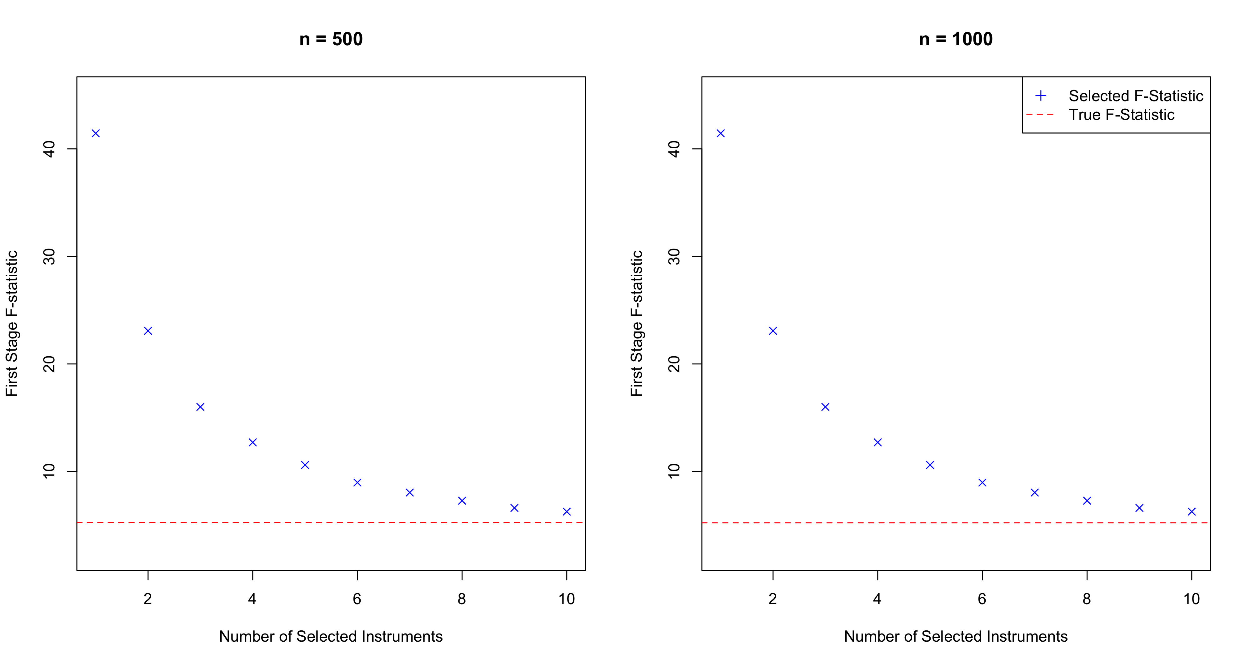
Figure 6.1: Results from Simulation Experiment. The endogenous variable is generated to be weakly related to a set of ten initial instruments. I take quadratic powers and interactions of these ten initial instruments to create an additional 55 technical instruments that do not directly enter the first stage. The LASSO penalty is then set to select a certain number of variables and I report the resulting average post-LASSO F-statistics over 1000 simulations. The average F-statistic using only the relevant ten initial instruments is 5.234 for both $n=500$ and $n=1000$.

Figure 6.2: First-Stage F-statistic as Function of Number of LASSO-Selected Variables in the Data of Gilchrist and Sands (2016). When selecting variables using a cross-validated choice of LASSO penalty parameter, the first-stage F-statistic is 6.42.

Given a lack of clarity on the strength of identification, I seek to validate the results of Gilchrist and Sands (2016) using the weak identification testing procedures proposed in this paper. The setting is particularly suitable for weak IV testing using the jackknife K-statistic. With 48 instruments and a sample size of 1671, $d_{z}^{3}=110{,}592\gg n$, making the tests of Moreira (2003, 2009); Kleibergen (2005), and Andrews (2016) inapplicable. On the other hand, it is unclear whether asymptotic approximations based on $d_{z}\to\infty$ will accurately describe the finite-sample distribution of test statistics with 48 instruments. Moreover, since fluctuations in movie theater attendance seem to be largely driven by either particularly cold or particularly hot weather (see Figure 4 in Gilchrist and Sands (2016)), the nuisance parameter $\rho(z_{i})$ is plausibly approximately sparse.Table 6.1 compares the $95\%$ confidence intervals for $\beta_{1},\dots,\beta_{7}$ generated by the jackknife K test to the confidence intervals generated by the sup-score test of Belloni et al. (2012) and the jackknife LM test (JLM) test of Matsushita and Otsu (2022). I form these confidence intervals by running the tests for each $\beta_{0}$ on a 300 point grid between zero and two and inverting the results; a point $\beta_{0}$ is included in the $95\%$ confidence interval if the test fails to reject the null that $\beta_{w}=\beta_{0}$ at level $\alpha=0.05$.For the $\text{\it JK}(\beta_{0})$ statistic I use the choice of hat matrix in (2.3) and estimate the auxiliary parameter $\rho(z_{i})$ as in (2.2). The penalty parameter $\lambda$ is chosen with leave-one-out cross-validation using the cv.glmnet command from the glmnet package in R (R Core Team, 2021; Friedman et al., 2010). The critical value for the sup-score statistic $S(\beta_{0})$ is simulated using 2,500 bootstrap draws. Confidence intervals based on the combination test, $T(\beta_{0};\tau)$, are not directly reported as the pretesting procedure based on simulating the 75^th quantile of $C$ as in (4.4) always suggests using the $\text{\it JK}(\beta_{0})$ statistic.For reference, I also provide point estimates and standard errors for $\beta_{1},\dots,\beta_{7}$ from Gilchrist and Sands (2016), Table 2. To facilitate comparison, these point estimates and standard errors come from a specification that uses all the instruments in the first stage of a 2SLS procedure. While the Gilchrist and Sands (2016) point estimates are always in the 95% confidence intervals generated by the $\text{\it JK}(\beta_{0})$ and JLM tests, the confidence intervals from the identification-robust procedures are significantly wider than those generated with the 2SLS standard errors.Interestingly, the confidence intervals from inverting the jackknife K-test tend to be quite similar to the confidence intervals from the JLM test. This is surprising given the distinct forms of the $\text{\it JK}(\beta_{0})$ and the JLM test statistics.For the parameters $\beta_{2},\beta_{4},\beta_{5},$ and $\beta_{6}$, the confidence intervals generated by the sup-score statistic are empty while the sup-score confidence interval for $\beta_{2}$ is nearly empty. This is also the case when using the jackknife AR-statistic of Crudu et al. (2021) and Mikusheva and Sun (2021), whose confidence intervals are not reported as they are always empty. With 48 instruments and a single parameter the linear IV model in (6.1) is overidentified and as such the empty confidence intervals could be interpreted as evidence of model misspecification. For the parameter $\beta_{7}$ the confidence interval generated by inverting the sup-score statistic is not empty and is instead 36% larger than the $\text{\it JK}(\beta_{0})$ confidence interval and 41% larger than the JLM confidence interval. This result suggests that the jackknife K tests and JLM tests may have better power properties than the sup-score test in this setting.

Parameter	$\beta_{2}$	$\beta_{3}$	$\beta_{4}$	$\beta_{5}$	$\beta_{6}$	$\beta_{7}$
$\underset{\text{(s.e.)}}{\text{Estimate}}$	$\underset{(0.024)}{0.475}$	$\underset{(0.023)}{0.269}$	$\underset{(0.017)}{0.164}$	$\underset{(0.013)}{0.121}$	$\underset{(0.010)}{0.093}$	$\underset{(0.074)}{1.222}$
$\text{\it JK}(\beta_{0})$	$[0.436,0.557]$	$[0.227,0.334]$	$[0.134,0.214]$	$[0.100,0.167]$	$[0.080,0.134]$	$[1.003,1.391]$
$S(\beta_{0})$	$\emptyset$	$[0.294,0.334]$	$[0.087,0.094]$	$\emptyset$	$\emptyset$	$[0.990,1.518]$
JLM	$[0.436,0.557]$	$[0.227,0.334]$	$[0.134,0.214]$	$[0.107,0.167]$	$[0.087,0.134]$	$[1.010,1.384]$

Table 6.1: 95% Confidence Intervals based on inverting various test statistics. Instrument set used is the same as the Gilchrist and Sands (2016) instrument set less four collinear instruments; $d_{z}=48$ with $n=1,671$. Thresholding test confidence intervals are not reported as they coincide with confidence intervals for $\text{\it JK}(\beta_{0})$.

Tables 6.2 and 6.3 repeat the analysis of Table 6.1 but with alternative instrument sets. The confidence intervals of Table 6.2 use only $5^{\circ}$ Fahrenheit temperature bins ($d_{z}=36$) while the confidence intervals of Table 6.3 include all the instruments used in Table 6.1 and all interactions between the $5^{\circ}$ Fahrenheit temperature bins and the other weather measures for a total of 524 instruments. For the most part, the confidence intervals generated by inverting the jackknife K-statistic are similar across Tables 6.1-6.3. The confidence intervals for the jackknife LM statistic however, become much narrower when using the largest set of instruments is used. Thisis interesting as the results from the $\text{\it JK}(\beta_{0})$ test as well as the power analysis in Section 4 seem to suggest that use of the extra isntruments does not lead to better first-stage estimates. Interestingly, the JLM confidence intervals in for $\beta_{6},\beta_{7}$ in Table 6.3 do not contain the point estimates for $\beta_{6}$ and $\beta_{7}$ from Gilchrist and Sands (2016). As with Table 6.1, Tables 6.2 and 6.3 do not report confidence intervals from $T(\beta_{0};\tau)$ as these always agree with the $\text{\it JK}(\beta_{0})$ confidence intervals and do not report jackknife AR confidence intervals as these are always empty.

Parameter	$\beta_{2}$	$\beta_{3}$	$\beta_{4}$	$\beta_{5}$	$\beta_{6}$	$\beta_{7}$
$\underset{\text{(s.e.)}}{\text{Estimate}}$	$\underset{(0.024)}{0.475}$	$\underset{(0.023)}{0.269}$	$\underset{(0.017)}{0.164}$	$\underset{(0.013)}{0.121}$	$\underset{(0.010)}{0.093}$	$\underset{(0.074)}{1.222}$
$\text{\it JK}(\beta_{0})$	$[0.449,0.597]$	$[0.255,0.389]$	$[0.148,0.248]$	$[0.114,0.194]$	$[0.094,0.154]$	$[1.086,1.555]$
$S(\beta_{0})$	$\emptyset$	$[0.302,0.329]$	$\emptyset$	$\emptyset$	$\emptyset$	$\emptyset$
JLM	$[0.449,0.597]$	$[0.255,0.389]$	$[0.154,0.248]$	$[0.114,0.194]$	$[0.094,0.154]$	$[1.092,1.555]$

Table 6.2: 95% Confidence Intervals based on inverting various test statistics. Instrument set used includes only temperatures measures; $d_{z}=36$, with $n=1,671$. Thresholding test condidence intervals are not reported as they coincide with confidence intervals for $\text{\it JK}(\beta_{0})$.

Parameter	$\beta_{2}$	$\beta_{3}$	$\beta_{4}$	$\beta_{5}$	$\beta_{6}$	$\beta_{7}$
$\underset{\text{(s.e.)}}{\text{Estimate}}$	$\underset{(0.024)}{0.475}$	$\underset{(0.023)}{0.269}$	$\underset{(0.017)}{0.164}$	$\underset{(0.013)}{0.121}$	$\underset{(0.010)}{0.093}$	$\underset{(0.074)}{1.222}$
$\text{\it JK}(\beta_{0})$	$[0.443,0.604]$	$[0.215,0.342]$	$[0.094,0.228]$	$[0.087,0.154]$	$[0.054,0.121]$	$[0.916,1.435]$
$S(\beta_{0})$	$[0.416,0.477]$	$\emptyset$	$\emptyset$	$[0.034,0.121]$	$[0.121,0.208]$	$[0.918,1.562]$
JLM	$[0.463,0.497]$	$[0.268,0.282]$	$[0.161,0.174]$	$[0.101,0.107]$	$[0.063,0.084]$	$[1.059,1.137]$

Table 6.3: 95% Confidence Intervals based on inverting various test statistics. Instrument set used includes the original instrument set along with interactions of the temperature measures set with all other aggregated weather measures; $d_{z}=524$, with $n=1,671$. Thresholding test confidence intervals are not reported as they coincide with confidence intervals for $\text{\it JK}(\beta_{0})$.

7 Simulation Study

In this simulation study, I examine the performance of tests based on the $\text{\it JK}(\beta_{0})$ statistic and compare it with that of other tests that may be used in settings where the number of instruments is nonnegligible as a fraction of sample size. I consider a reduced-form data-generating process (DGP) similar to that of Matsushita and Otsu (2022). The outcome variable, $y_{i}$, and endogenous variable, $x_{i}$, are generated according to

$$\begin{split}y_{i}&=x_{i}+\epsilon_{i}\\ x_{i}&={}_{i}+v_{i}\end{split}$$ (7.1)

where ${}_{i}=\frac{1}{r_{n}}\sumop\slimits@_{k=1}^{5}\frac{3}{4}\bar{z}_{ki}+\frac{1}{4}\bar{z}_{ki}^{2}+\frac{1}{4}\bar{z}_{ki}^{3}$ is a transformation of an initial set of instruments $\bar{z}_{i}\in\mathbb{R}^{10}$ generated as described below. The value of $r_{n}$ varies depending on the strength of identification considered; for strong identification, $r_{n}=1$, while under weak identification, $r_{n}=1/\sqrt{n}.$To model heteroskedasticity, the errors $(e_{i},v_{i})$ are generated $\epsilon_{i}=(1+\varrho_{1}(\bar{z}_{1i}^{2}+\bar{z}_{2i}^{2}+\bar{z}_{2i}\bar{z}_{3i}))e_{1i}$, and $v_{i}=\varrho_{2}(1+\bar{z}_{1i})\epsilon_{i}+(1-\varrho_{2})^{2}e_{2i}$ where $e_{1i}$ and $e_{2i}$ are generated independently of each other and other variables in the model according to a Laplace distribution with location parameter $\mu=0$ and scale parameter $b=1$. Since the limiting $\chi^{2}$ distribution of the jackknife K-statistic is exact when the errors are jointly Gaussian and $\rho(z_{i})$ is known, I purposefully avoid normally distributed errors to investigate the quality of asymptotic approximations to the finite-sample behavior of the test. The parameters $\varrho_{1}$ and $\varrho_{2}$ control the degree of heteroskedasticity and endogeneity, respectively.

DGP				Testing Procedure
$n$	$d_{z}$	$\varrho_{1}$	$\varrho_{2}$	$\text{\it JK}(\beta_{0})$	$S(\beta_{0})$	$T(\beta_{0};\tau_{0.3})$	$T(\beta_{0};\tau_{0.75})$	A.Rbn.	JAR	JLM
200	10	0.2	0.3	0.0516	0.0352	0.0406	0.0406	0.0296	0.0766	0.0502
		0.2	0.6	0.0542	0.0306	0.0442	0.0384	0.0258	0.0748	0.0400
		0.5	0.3	0.0470	0.0338	0.0416	0.0418	0.0238	0.0784	0.0460
		0.5	0.6	0.0506	0.0350	0.0416	0.0390	0.0280	0.0676	0.0384
	30	0.2	0.3	0.0570	0.0124	0.0422	0.0200	0.0088	0.1000	0.0382
		0.2	0.6	0.0564	0.0126	0.0408	0.0208	0.0124	0.0962	0.0322
		0.5	0.3	0.0498	0.0100	0.0366	0.0190	0.0096	0.1090	0.0318
		0.5	0.6	0.0562	0.0118	0.0420	0.0216	0.0088	0.1104	0.0292
	65	0.2	0.3	0.0542	0.0316	0.0428	0.0370	0.0314	0.0764	0.0420
		0.2	0.6	0.0532	0.0366	0.0418	0.0398	0.0250	0.0780	0.0376
		0.5	0.3	0.0474	0.0308	0.0388	0.0362	0.0244	0.0748	0.0354
		0.5	0.6	0.0484	0.0324	0.0366	0.0388	0.0282	0.0708	0.0402
500	10	0.2	0.3	0.0590	0.0468	0.0478	0.0516	0.0376	0.0652	0.0452
		0.2	0.6	0.0530	0.0420	0.0460	0.0466	0.0366	0.0692	0.0434
		0.5	0.3	0.0496	0.0370	0.0408	0.0368	0.0338	0.0710	0.0464
		0.5	0.6	0.0512	0.0426	0.0456	0.0438	0.0334	0.0696	0.0404
	30	0.2	0.3	0.0522	0.0202	0.0386	0.0278	0.0238	0.0818	0.0322
		0.2	0.6	0.0558	0.0208	0.0408	0.0310	0.0266	0.0888	0.0342
		0.5	0.3	0.0554	0.0178	0.0392	0.0280	0.0174	0.0940	0.0272
		0.5	0.6	0.0570	0.0156	0.0426	0.0236	0.0206	0.0984	0.0280
	65	0.2	0.3	0.0542	0.0372	0.0434	0.0432	0.0384	0.0754	0.0464
		0.2	0.6	0.0584	0.0442	0.0482	0.0470	0.0334	0.0676	0.0438
		0.5	0.3	0.0614	0.0460	0.0504	0.0496	0.0316	0.0708	0.0434
		0.5	0.6	0.0526	0.0378	0.0434	0.0420	0.0298	0.0692	0.0358

Table 7.1: Simulated Size of Identification and Heteroskedasticity Robust Tests under Weak Identification. Each DGP is simulated 5000 times. Critical values of the sup-score statistic and quantiles of the conditioning statistic are calculated using 1000 multiplier bootstrap simulations.

DGP				Testing Procedure
$n$	$d_{z}$	$\varrho_{1}$	$\varrho_{2}$	$\text{\it JK}(\beta_{0})$	$S(\beta_{0})$	$T(\beta_{0};\tau_{0.3})$	$T(\beta_{0};\tau_{0.75})$	A.Rbn.	JAR	JLM
200	10	0.2	0.3	0.0474	0.0420	0.0474	0.0468	0.0308	0.0728	0.0424
		0.2	0.6	0.0512	0.0386	0.0512	0.0506	0.0304	0.0764	0.0378
		0.5	0.3	0.0416	0.0318	0.0414	0.0414	0.0248	0.0794	0.0428
		0.5	0.6	0.0446	0.0342	0.0446	0.0442	0.0244	0.0806	0.0384
	30	0.2	0.3	0.0482	0.0122	0.0448	0.0264	0.0110	0.1048	0.0370
		0.2	0.6	0.0498	0.0120	0.0480	0.0312	0.0118	0.0980	0.0378
		0.5	0.3	0.0456	0.0126	0.0410	0.0262	0.0082	0.1146	0.0268
		0.5	0.6	0.0482	0.0110	0.0474	0.0308	0.0094	0.1090	0.0302
	65	0.2	0.3	0.0528	0.0380	0.0526	0.0510	0.0276	0.0696	0.0460
		0.2	0.6	0.0464	0.0360	0.0464	0.0468	0.0302	0.0728	0.0416
		0.5	0.3	0.0482	0.0298	0.0480	0.0466	0.0246	0.0738	0.0412
		0.5	0.6	0.0396	0.0320	0.0390	0.0386	0.0258	0.0748	0.0356
500	10	0.2	0.3	0.0524	0.0444	0.0524	0.0524	0.0394	0.0684	0.0472
		0.2	0.6	0.0476	0.0430	0.0476	0.0476	0.0400	0.0644	0.0490
		0.5	0.3	0.0434	0.0410	0.0434	0.0434	0.0340	0.0702	0.0404
		0.5	0.6	0.0448	0.0382	0.0448	0.0448	0.0350	0.0736	0.0432
	30	0.2	0.3	0.0502	0.0214	0.0502	0.0498	0.0240	0.0854	0.0368
		0.2	0.6	0.0522	0.0208	0.0522	0.0524	0.0224	0.0858	0.0392
		0.5	0.3	0.0456	0.0202	0.0456	0.0434	0.0220	0.0918	0.0264
		0.5	0.6	0.0500	0.0186	0.0500	0.0498	0.0204	0.0924	0.0268
	65	0.2	0.3	0.0490	0.0426	0.0490	0.0490	0.0350	0.0742	0.0472
		0.2	0.6	0.0522	0.0458	0.0522	0.0522	0.0436	0.0652	0.0442
		0.5	0.3	0.0542	0.0476	0.0542	0.0542	0.0294	0.0712	0.0446
		0.5	0.6	0.0438	0.0420	0.0438	0.0438	0.0306	0.0666	0.0500

Table 7.2: Simulated Size of Identification and Heteroskedasticity Robust Tests under Strong Identification. Each DGP is simulated 5000 times. Critical values of the sup-score statistic and quantiles of the conditioning statistic are calculated using 1000 multiplier bootstrap simulations.

In addition to considering the behavior of tests under both weak and strong identification, I examine the size of the test under three different instrument regimes. In all three regimes, I begin with an initial set of instruments $\bar{z}_{i}=(\bar{z}_{1i},\dots,\bar{z}_{10i})^{\prime}$ generated independently across indices according to a multivariate Gaussian distribution with Toeplitz covariance structure, $\operatorname{Cov}(\bar{z}_{\ell i},\bar{z}_{ki})=2^{-|\ell-k|}$. In the first regime, the full set instruments $z_{i}$ is taken to be equal to $\bar{z}_{i}$ so that $d_{z}=10$. In the second regime, the full set of instruments $z_{i}$ additionally includes all quadratic and cubic terms, $(z_{\ell i}^{2},z_{\ell i}^{3})$, $\ell=1,\dots,10$ so that in total $d_{z}=30$. In the third regime, the full set of instrument includes the initial set of instruments, $\bar{z}_{i}$, and all quadratic terms (10 additional terms) and interactions of the initial set of instruments ($\binom{10}{2}=45$additional terms), so that in total $d_{z}=65$. Under each regime, the full set of instruments is passed to the test statistics with no indication about which instruments correspond to the initial set, and thus no indication about which instruments are relevant to the DGP.

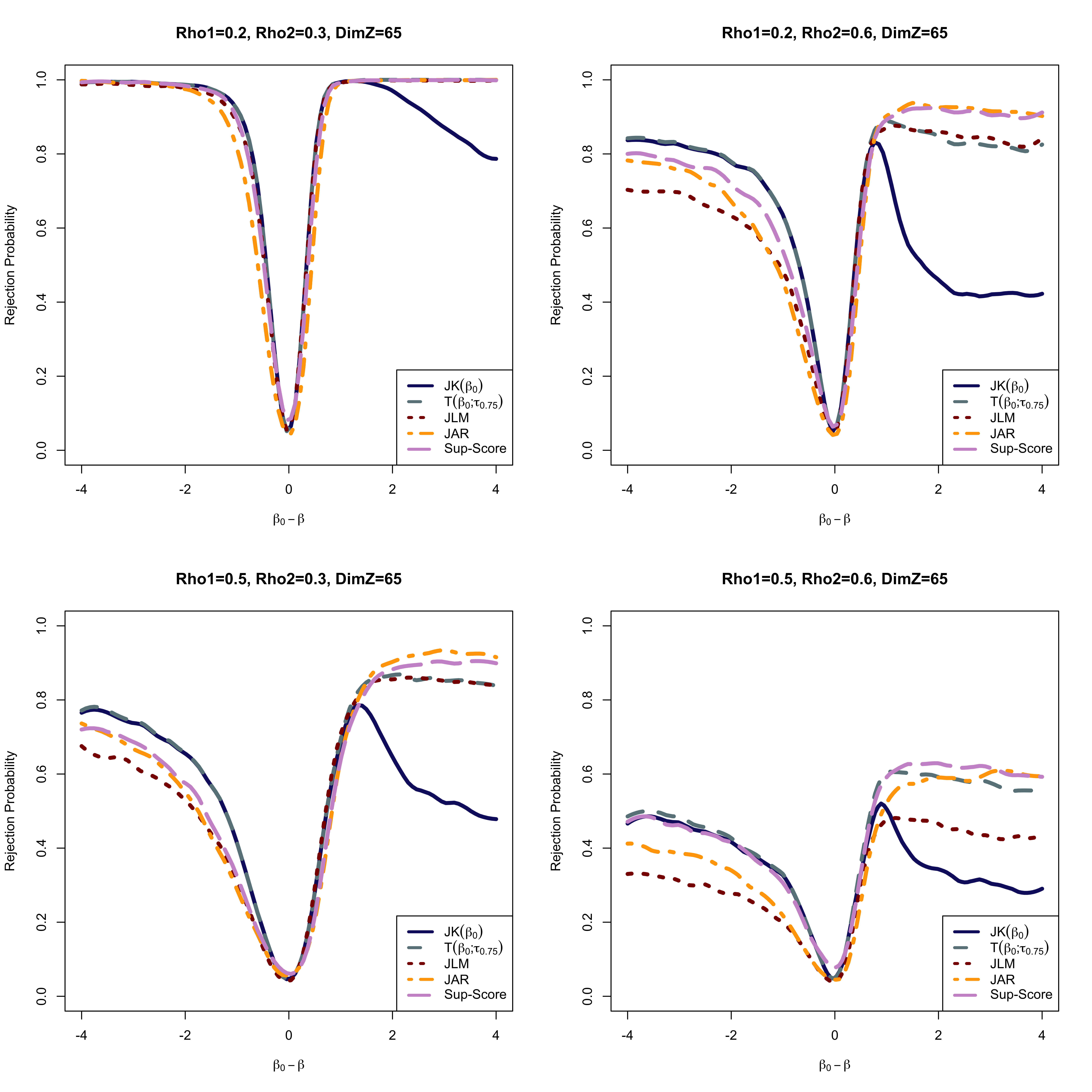
Figure 7.1: Calibrated Local Power Curves under Intermediate Identification Strength and 65 Instruments. Sample size is 500 and rejection probability is calculated on a grid of 100 $(\beta_{0}-\beta)$ points between -4 and 4. At each point the DGP is simulated 2000 times.

I compare the simulated size of the jackknife K test and to the performance of the sup-score test, $S(\beta_{0})$, of Belloni et al. (2012), the thresholding test introduced in Section 4.2, the standard Anderson-Rubin (A.Rbn.) test of Anderson and Rubin (1949) and Staiger and Stock (1997), the jackknife AR test (JAR) of Crudu et al. (2021) and Mikusheva and Sun (2021), and the jackknife LM test (JLM) of Matsushita and Otsu (2022). To estimate the parameter $\rho(z_{i})$, I implement the $\ell_{1}$-penalized procedure of (2.2) via the glmnet package in R (Friedman et al., 2010). The penalty parameter $\lambda$ is selected via tenfold cross-validation. I use the full vector of instruments as the basis to approximate $\rho(z_{i})$. For the jackknife AR test I use cross-fit estimates of test statistic variances proposed and shown to improve power by Mikusheva and Sun (2021).Critical values of the sup-score and conditioning statistic are simulated with the procedures described in Section 4 with 1000 bootstrap replications. For the combination test cutoff, I consider two different quantiles of the conditioning statistic under the assumption that $\mathbb{E}[\mathaccent 0{\symlargesymbols}062{}_{i}^{I}]=0$ for all $i\in[n]$; $\tau_{0.3}$ corresponding to the 30^th quantile and $\tau_{0.75}$ corresponding to the 75^th quantile.Tables 7.1 and 7.2 report the simulated size for all tests under weak and strong identification, respectively. One can see that the $\text{\it JK}(\beta_{0})$ statistic has nearly exact size in almost all the setups considered. In contrast, the jackknife AR test seems to overreject in nearly all the simulation setups considered. This is also the case in the simulation study of Matsushita and Otsu (2022) and so may be an artifact of the similarity of my simulation design to theirs.The sup-score, jackknife AR, and jackknife LM test all seem to have particularly poor performance under both weak and strong identification when $d_{z}=30$. This is the setup with the most correlation between the instruments. While tests based on the jackknife AR statistic can have a simulated size that is nearly double the nominal size in this setting, both the sup-score and and jackknife LM tests appear to be conservative. The size of the sup-score test is always under $0.025$ while the size of the JLM test can be under half of the nominal size. Notably, the size properties of the sup-score test do seem to improve under both weak and strong identification when the sample size increases from $n=200$ to $n=500$. This is in line with theoretical results showing that the sup-score test has exact asymptotic size under standard conditions. In contrast, the size properties of the jackknife LM test do not seem to improve when the sample size increases and indeed worsen for three out of the four DGPs considered under both weak and strong identification. This suggests that the requirement of $d_{z}\to\infty$ may be important for the quality of finite-sample approximation by its limiting distribution.The thresholding test seems to control size in all the setups considered. However, under weak identification the thresholding test appears to inherit the conservative nature of the sup-score test, even in the “large” sample size regime of $n=500$. This is not the case under strong identification, suggesting that the thresholding-test is choosing to run tests based on the $\text{\it JK}(\beta_{0})$ with high probability in this regime. This behavior is similar to the conditional combination tests of Moreira (2003); Andrews (2016) which weigh the K-statistic more under strong identification. This behavior is optimal as the K-statistic yields effecient inference when the data is informative about the structural parameter (Andrews et al., 2004, 2006). When errors are homoskedastic and the number of instruments is fixed, the jackknife K-statistic can also be shown to yield effecient inference under strong identification.

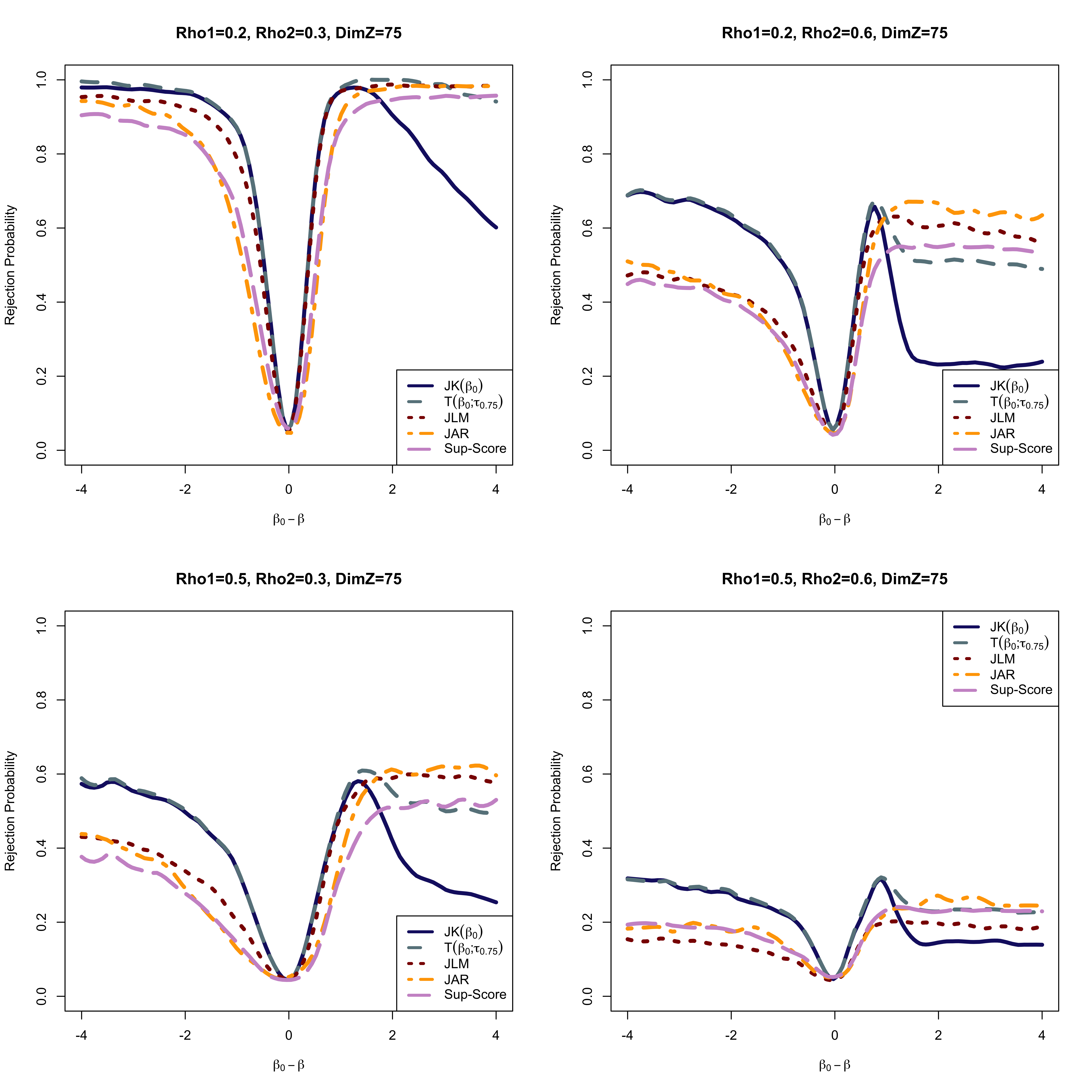
Figure 7.2: Calibrated Local Power Curves under Intermediate identification Strength and 75 Instruments. Sample size is 500 and rejection power is calculated on a grid of 100 $(\beta_{0}-\beta)$ points between -4 and 4. At each point the DGP is simulated 2000 times.

Figure 7.1 plots calibrated local power curves under an intermediate-strength identification where the first stage is in a $n^{-1/3}$ neighborhood of zero, $d_{z}=65$, $\varrho_{1}\in\{0.2,0.5\}$ and $\varrho_{2}\in\{0.3,0.6\}$. The critical value of each test is set to simulated 95^th quantile of the distribution of the corresponding test-statistic under $H_{0}$. I compare the calibrated local power curves of the $\text{\it JK}(\beta_{0})$ test, the combination test with cutoff $\tau_{0.75}$, the jackknife AR test, the Jackknife LM test, and the sup-score test. The jackknife K-test appears to have stronger power than the jackknife AR, jackknife LM, and sup-score tests in local neighborhoods of the null as well as for negative values of $(\beta_{0}-\beta)$. For values of $(\beta_{0}-\beta)$ larger than 1.5, tests based on the jackknife K-statistic appear to suffer from a loss of power as described inSection 4. This power decline appears to be largerly ameliorated by combining the jackknife K-statistic with the sup-score statistic and the thresholding test appears to have good power properties over all alternatives considered. However, tests based on the jackknife AR or jackknife LM statistic may still provide better power than the threshholding test for very positive values of $(\beta_{0}-\beta)$.In order to consider the effect of correlated instruments on the power properties of the test in a setting with plausibly many instruments, I additionally examine local power under a fourth instrument regime. This setup adds the ten cubic terms $z_{\ell i}^{3},\ell=1,\dots,10$ to the interactions and quadratic terms of the third instrument regime for a total of 75 instruments, $d_{z}=75$. Appendix I provides the simulated sizes of tests under this fourth regime. Figure 7.2 plots calibrated local power curves under this fourth instrument regime. While all tests have lower power in this regime than in the regime considered in Figure 7.1, the many instrument jackknife AR and jackknife LM tests appear to face a steeper power decline than tests based on the jackknife K-statistic or the thresholding statistic.These results should not be interpreted as critiques of the benchmark testing procedures of Anderson and Rubin (1949); Staiger and Stock (1997); Belloni et al. (2012); Crudu et al. (2021); Mikusheva and Sun (2021), and Matsushita and Otsu (2022), whose work I rely on and was inspired by.

8 Conclusion

I propose a new test for the structural parameter in a linear instrumental variables model. This test is based on a jackknife version of the K-statistic and the limiting behavior of the test is analyzed via a novel direct Gaussian approximation argument. I show that, as long as an auxiliary parameter can be consistently estimated, the test is robust to both the strength of identification and the number of instruments; the limiting distribution of the test statistic does not depend on either of these factors. Consistency of the auxiliary parameter can be achieved under approximate sparsity using simple-to-implement $\ell_{1}$-penalized methods.I characterize the behavior of the jackknife K-statistic in local neighborhoods of the null. To address a power deficiency that tests based on jackknife K-statistic inherit from their non-jackknife namesakes, I propose a testing procedure that decides whether the researcher should run a test via the jackknife K-statistic or one via the sup-score statistic based on the value of a conditioning statistic. While this combination does not fully address the power decline, I show that it works well in a simulation study and leave further refinements to future work.

Appendix A Proofs of Results in Section 3

A.1 Proof of Lemma 3.1

The statement $\sup_{a<0}\big{|}\mathrm{Pr}(\text{\it JK}_{I}(\beta_{0})\leq a)-\mathrm{Pr}(\text{\it JK}_{G}(\beta_{0})\leq a)\big{|}=0$ is immediate since both $\text{\it JK}_{I}(\beta_{0})$ and $\text{\it JK}_{G}(\beta_{0})$ are always weakly positive.It thus suffices to show

$$\sup_{a\geq 0}\big{|}\mathrm{Pr}(\text{\it JK}_{I}(\beta_{0})\leq a)-\mathrm{Pr}(\text{\it JK}_{G}(\beta_{0})\leq a)\big{|}\to 0$$

Before proceeding, we will introduce some notation. Let $\tilde{H}=s_{n}H$ and $\tilde{h}_{ij}=s_{n}h_{ij}$, where $s_{n}$ is as in Assumption 3.2. Recall that $\tilde{h}_{ii}=0$ and define

$$N \mathrel{\mathop{\ordinarycolon}}=\frac{1}{\sqrt{n}}\sumop\slimits@_{i=1}^{n}\epsilon_{i}(\beta_{0})\sumop\slimits@_{j=1}^{n}\tilde{h}_{ij}r_{j} \mathrel{\mathop{\ordinarycolon}}=\frac{1}{\sqrt{n}}\sumop\slimits@_{i=1}^{n}\tilde{\epsilon}_{i}(\beta_{0})\sumop\slimits@_{j=1}^{n}\tilde{h}_{ij}\tilde{r}_{j}$$

$$D \mathrel{\mathop{\ordinarycolon}}=\frac{1}{n}\sumop\slimits@_{i=1}^{n}\epsilon_{i}^{2}(\beta_{0})\big{(}\sumop\slimits@_{j=1}^{n}\tilde{h}_{ij}r_{j}\big{)}^{2} \mathrel{\mathop{\ordinarycolon}}=\frac{1}{n}\sumop\slimits@_{i=1}^{n}\kappa_{i}^{2}(\beta_{0})\big{(}\sumop\slimits@_{j=1}^{n}\tilde{h}_{ij}\tilde{r}_{j}\big{)}^{2}$$

where $(\tilde{\epsilon}_{i}(\beta_{0}),\tilde{r}_{i})$ are jointly Gaussian with the same mean and covariance matrix as $(\epsilon_{i}(\beta_{0}),r_{i})$ and $\kappa_{i}^{2}(\beta_{0})=\mathbb{E}[\epsilon_{i}^{2}(\beta_{0})]$.Under this notation we can write $\text{\it JK}_{I}(\beta_{0})=\frac{N^{2}}{D}\bm{1}_{\{D>0\}}$ and $\text{\it JK}_{G}(\beta_{0})=\frac{\tilde{N}^{2}}{\tilde{D}}$. Dealing with these forms of the statistics is difficult for the interpolation argument, since the denominator is random. Instead, we will notice that since $D=0\implies N=0$ and $\mathrm{Pr}(\tilde{D}>0)=1$, for any $a\geq 0$ we can rewrite the events

$$\begin{split}\{\text{\it JK}_{I}(\beta_{0})\leq a\}=\{N^{2}-aD\leq 0\}\hbox{ }\text{ and }\hbox{ }\{\text{\it JK}_{G}(\beta_{0})\leq a\}\overset{\text{a.s}}{=}\{\tilde{N}^{2}-a\tilde{D}\leq 0\}\end{split}$$ (A.1)

With this in mind define

$$\text{\it JK}^{a}\mathrel{\mathop{\ordinarycolon}}=N^{2}-aD\hbox{ }\text{ and }\hbox{ }\tilde{\text{\it JK}}^{a}\mathrel{\mathop{\ordinarycolon}}=\tilde{N}^{2}-a\tilde{D}$$

Showing Lemma 3.1 is then equivalent to showing that $\sup_{a}|\mathrm{Pr}(\text{\it JK}^{a}\leq 0)-\mathrm{Pr}(\tilde{\text{\it JK}}^{a}\leq 0)|\to 0$. We do so in a few lemmas, the final result being shown in Lemma A.6 at the bottom of this subsection.

Lemma A.1 (Lindeberg Interpolation).

Suppose that Assumptions 3.1, 3.2 and 3.3 hold. Let $\varphi(\cdot)\mathrel{\mathop{\ordinarycolon}}\mathbb{R}\to\mathbb{R}$ be such that $\varphi(\cdot)\in C_{b}^{3}(\mathbb{R})$ with $L_{2}(\varphi)=\sup_{x}|\varphi^{\prime\prime}(x)|$ and $L_{3}(\varphi)=\sup_{x}|\varphi^{\prime\prime\prime}(x)|$. Then, there is a constant $M$ that depends only on the constant $c$ such that:

$$|\mathbb{E}[\varphi(\text{\it JK}^{a})-\varphi(\tilde{\text{\it JK}}^{a})]|\leq\frac{M(a^{3}\vee 1)}{\sqrt{n}}(L_{2}(\varphi)+L_{3}(\varphi))$$

Proof of Lemma A.1.

Begin by defining the leave-one-out numerator, denominator, and decomposed statistics

$$N_{-i} \mathrel{\mathop{\ordinarycolon}}=\frac{1}{\sqrt{n}}\sumop\slimits@_{j\neq i}\dot{\epsilon}_{j}(\beta_{0})\sumop\slimits@_{\ell\neq i}\tilde{h}_{j\ell}\dot{r}_{\ell} D_{-i} \mathrel{\mathop{\ordinarycolon}}=\frac{1}{n}\sumop\slimits@_{j\neq i}\ddot{\epsilon}_{j}^{2}(\beta_{0})\big{(}\sumop\slimits@_{\ell\neq i}\tilde{h}_{j\ell}\dot{r}_{\ell}\big{)}^{2}$$

$$\text{\it JK}_{-i} \mathrel{\mathop{\ordinarycolon}}=N_{-i}^{2}-aD_{-i}$$

where for each $\ell\in[n]$, $\dot{\epsilon}_{\ell}(\beta_{0})$ is equal to $\epsilon_{\ell}(\beta_{0})$ if $\ell>i$ and $\tilde{\epsilon}_{\ell}(\beta_{0})$ if $\ell<i$, $\dot{r}_{\ell}$ is equal to $r_{\ell}$ if $\ell>i$ and $\tilde{r}_{\ell}$ if $\ell<i$, and $\ddot{\epsilon}_{\ell}^{2}(\beta_{0})$ is equal to $\kappa_{\ell}^{2}(\beta_{0})$ if $\ell<i$ and $\epsilon_{\ell}^{2}(\beta_{0})$ if $\ell>i$. While the definitions of $\dot{\epsilon}_{\ell},\dot{r}_{\ell},$ and $\ddot{\epsilon}_{\ell}$ depend on $i$ because we will be considering only one deviation at a time, we will supress the dependence of these variables on $i$ to simplify notation.Next, define the one-step deviations

$$\begin{split}{}_{1i}&\mathrel{\mathop{\ordinarycolon}}=\epsilon_{i}(\beta_{0})\sumop\slimits@_{j=1}^{n}\tilde{h}_{ij}\dot{r}_{j}+r_{i}\sumop\slimits@_{j=1}^{n}\tilde{h}_{ji}\dot{\epsilon}_{j}(\beta_{0})\\ \tilde{\Delta}_{1i}&\mathrel{\mathop{\ordinarycolon}}=\tilde{\epsilon}_{i}(\beta_{0})\sumop\slimits@_{j=1}^{n}\tilde{h}_{ij}\dot{r}_{j}+\tilde{r}_{i}\sumop\slimits@_{j=1}^{n}\tilde{h}_{ji}\dot{\epsilon}_{j}(\beta_{0})\\ {}_{2i}&\mathrel{\mathop{\ordinarycolon}}=\underbrace{a\epsilon_{i}^{2}(\beta_{0})(\sumop\slimits@_{j=1}^{n}\tilde{h}_{ij}\dot{r}_{j})^{2}+ar_{i}^{2}\sumop\slimits@_{j=1}^{n}\tilde{h}_{ji}^{2}\ddot{\epsilon}_{j}^{2}(\beta_{0})}_{{}_{2i}^{a}}+\underbrace{2ar_{i}\sumop\slimits@_{j=1}^{n}\ddot{\epsilon}_{j}^{2}(\beta_{0})\sumop\slimits@_{\ell\neq i}\tilde{h}_{j\ell}\tilde{h}_{ji}\dot{r}_{\ell}}_{{}_{2i}^{b}}\\ \tilde{\Delta}_{2i}&\mathrel{\mathop{\ordinarycolon}}=\underbrace{a\kappa_{i}^{2}(\beta_{0})(\sumop\slimits@_{j=1}^{n}\tilde{h}_{ij}\dot{r}_{j})^{2}+a\tilde{r}_{i}^{2}\sumop\slimits@_{j=1}^{n}\tilde{h}_{ji}^{2}\ddot{\epsilon}_{j}^{2}(\beta_{0})}_{{}_{2i}^{a}}+\underbrace{2a\tilde{r}_{i}\sumop\slimits@_{j=1}^{n}\ddot{\epsilon}_{j}^{2}(\beta_{0})\sumop\slimits@_{\ell\neq i}\tilde{h}_{j\ell}\tilde{h}_{ji}\dot{r}_{\ell}}_{\tilde{\Delta}_{2i}^{b}}\end{split}$$ (A.2)

These one-step deviations contain all the terms associated with observation $i$ in the expression of the numerator and denominator of the test statistics. To demonstrate, note that these one-step deviations satisfy $N_{-1}+n^{-1/2}{}_{11}=N$ and $aD_{-1}+n^{-1}{}_{21}=aD$ as

$$N =\frac{1}{\sqrt{n}}\sumop\slimits@_{i=1}^{n}\epsilon_{i}(\beta_{0})\sumop\slimits@_{j=1}^{n}\tilde{h}_{ij}r_{j}$$

$$=\frac{1}{\sqrt{n}}\sumop\slimits@_{j>1}\epsilon_{j}(\beta_{0})\sumop\slimits@_{\ell=1}^{n}\tilde{h}_{j\ell}r_{j}+\epsilon_{1}(\beta_{0})\frac{1}{\sqrt{n}}\sumop\slimits@_{j>1}\tilde{h}_{1j}r_{j}$$

$$=\frac{1}{\sqrt{n}}\sumop\slimits@_{j>1}\epsilon_{j}(\beta_{0})\Big{\{}\tilde{h}_{j1}r_{1}+\sumop\slimits@_{\ell>1}h_{j\ell}r_{\ell}\Big{\}}+\epsilon_{1}(\beta_{0})\frac{1}{\sqrt{n}}\sumop\slimits@_{j>1}\tilde{h}_{1j}r_{j}$$

$$=\underbrace{\frac{1}{\sqrt{n}}\sumop\slimits@_{j>1}\epsilon_{j}(\beta_{0})\sumop\slimits@_{\ell>1}h_{j\ell}r_{\ell}}_{N_{-1}}+\underbrace{\epsilon_{1}(\beta_{0})\frac{1}{\sqrt{n}}\sumop\slimits@_{j>1}\tilde{h}_{1j}r_{j}+r_{1}\frac{1}{\sqrt{n}}\sumop\slimits@_{j>1}\tilde{h}_{j1}\epsilon_{j}(\beta_{0})}_{n^{-1/2}{}_{11}}$$

and

$$D =\frac{1}{n}\sumop\slimits@_{i=1}^{n}\epsilon_{i}^{2}(\beta_{0})\big{(}\sumop\slimits@_{j=1}^{n}\tilde{h}_{ij}r_{j})^{2}$$

$$=\frac{1}{n}\sumop\slimits@_{j>1}\epsilon_{j}^{2}(\beta_{0})\big{(}\sumop\slimits@_{\ell=1}^{n}\tilde{h}_{j\ell}r_{\ell}\big{)}^{2}+\epsilon_{1}^{2}(\beta_{0})\frac{1}{n}\big{(}\sumop\slimits@_{j>1}\tilde{h}_{1j}r_{j}\big{)}^{2}$$

$$=\frac{1}{n}\sumop\slimits@_{j>1}\epsilon_{j}^{2}(\beta_{0})\big{(}\tilde{h}_{j1}r_{1}+\sumop\slimits@_{\ell\neq 1}\tilde{h}_{\ell j}r_{\ell}\big{)}^{2}+\epsilon_{1}^{2}(\beta_{0})\frac{1}{n}\big{(}\sumop\slimits@_{j>1}\tilde{h}_{1j}r_{j}\big{)}^{2}$$

$$=\underbrace{\frac{1}{n}\sumop\slimits@_{j>1}\epsilon_{j}^{2}(\beta_{0})\big{(}\sumop\slimits@_{\ell>1}\tilde{h}_{\ell,j}r_{\ell}\big{)}^{2}}_{D_{-1}}$$

$$\;\;\;\;\;\;+\underbrace{\epsilon_{1}^{2}(\beta_{0})\frac{1}{n}\big{(}\sumop\slimits@_{j>1}\tilde{h}_{1j}r_{j}\big{)}^{2}+r_{1}^{2}\frac{1}{n}\sumop\slimits@_{j>1}\tilde{h}_{j1}^{2}\epsilon_{j}^{2}(\beta_{0})+2r_{1}\frac{1}{n}\sumop\slimits@_{j>1}\epsilon_{j}^{2}(\beta_{0})\sumop\slimits@_{\ell>1}\tilde{h}_{\ell j}r_{\ell}}_{(an)^{-1}{}_{21}}$$

Using the one-step deviations, write the difference $\mathbb{E}[\varphi(K^{a})-\varphi(\tilde{K}^{a})]$ as a telescoping sum, one by one replacing $({}_{1i},{}_{2i})$ with $(\tilde{\Delta}_{1i},\tilde{\Delta}_{2i})$ in the expressions of $\text{\it JK}^{a}=N^{2}-aD$ until we arrive at $\tilde{\text{\it JK}}^{a}=\tilde{N}^{2}-a\tilde{D}$.

$$\begin{split}\mathbb{E}[\varphi(\text{\it JK}^{a})-\varphi(\tilde{\text{\it JK}}^{a})]&=\sumop\slimits@_{i=1}^{n}\mathbb{E}[\varphi(\text{\it JK}_{-i}+n^{-1/2}N_{-i}{}_{1i}+n^{-1}{}_{1i}^{2}-n^{-1}{}_{2i})]\\ &\hphantom{=\sumop\slimits@_{i=1}^{n}\;\;}-\mathbb{E}[\varphi(\text{\it JK}_{-i}+n^{-1/2}N_{-i}\tilde{\Delta}_{1i}+n^{-1}\tilde{\Delta}_{1i}^{2}-n^{-1}\tilde{\Delta}_{2i})]\end{split}$$ (A.3)

Via a second-order Taylor expansion, we can write each term inside the summand

$$\mathbb{E}[\text{Term}_{i}] =\mathbb{E}[\varphi^{\prime}(\text{\it JK}_{-i})\{2n^{-1/2}N_{-i}({}_{1i}-\tilde{\Delta}_{1i})+n^{-1}({}_{1i}^{2}-{}_{1i}^{2})-n^{-1}({}_{2i}-\tilde{\Delta}_{2i})\}]$$

$$+\mathbb{E}[\varphi^{\prime\prime}(\text{\it JK}_{-i})\{4n^{-1}N_{-i}^{2}({}_{1i}^{2}-\tilde{\Delta}_{1i}^{2})+n^{-2}({}_{1i}^{4}-\tilde{\Delta}_{1i}^{4})-n^{-2}({}_{2i}^{2}-{}_{2i}^{2})\}]$$

$$+\mathbb{E}[\varphi^{\prime\prime}(\text{\it JK}_{-i})\{4n^{-3/2}N_{-i}({}_{1i}^{3}-\tilde{\Delta}_{1i}^{3})+4n^{-3/2}N_{-i}({}_{1i}{}_{2i}-\tilde{\Delta}_{1i}\tilde{\Delta}_{2i})\}]$$

$$+\mathbb{E}[\varphi^{\prime\prime}(\text{\it JK}_{-i})\{2n^{-2}({}_{1i}^{2}{}_{2i}-\tilde{\Delta}_{1i}^{2}\tilde{\Delta}_{2i})\}]+R_{i}+\tilde{R}_{i}$$

where $R_{i}$ and $\tilde{R}_{i}$ are remainder terms to be examined later. Let $\mathcal{F}_{-i}$ denote the sigma algebra generated by all random variables whose index is not equal to $i$. Since (a) for each $i\in[n]$ the mean and covariance matrix of $(\epsilon_{i}(\beta_{0}),r_{i})$ is the same as the mean and covariance matrix of $(\tilde{\epsilon}_{i}(\beta_{0}),\tilde{r}_{i})$, (b) $\mathbb{E}[\epsilon_{i}^{2}(\beta_{0})]=\kappa_{i}^{2}(\beta_{0})$, and (c) random variables are independent across indices, we have that

$$\begin{split}\mathbb{E}[{}_{1i}-\tilde{\Delta}_{1i}|\mathcal{F}_{-i}]&=\mathbb{E}[{}_{1i}^{2}-\tilde{\Delta}_{1i}^{2}|\mathcal{F}_{-i}]=\mathbb{E}[{}_{2i}-\tilde{\Delta}_{2i}|\mathcal{F}_{-i}]\\ &=\mathbb{E}[{}_{2i}^{b}-\tilde{\Delta}_{2i}^{b}|\mathcal{F}_{-i}]=\mathbb{E}[{}_{1i}{}_{2i}^{b}-\tilde{\Delta}_{1i}\tilde{\Delta}_{2i}^{b}|\mathcal{F}_{-i}]=0\end{split}$$ (A.4)

Using this we can simplify the prior display

$$\mathbb{E}[\text{Term}_{i}] =\underbrace{n^{-2}\mathbb{E}[\varphi^{\prime\prime}(\text{\it JK}_{-i})({}_{1i}^{4}-{}_{1i}^{4})]}_{\mathbf{A}_{i}}-\underbrace{n^{-2}\mathbb{E}[\varphi^{\prime\prime}(\text{\it JK}_{-i})(({}_{2i}^{a})^{2}-(\tilde{\Delta}_{2i}^{a})^{2})]}_{\mathbf{B}_{i}}$$

$$-\underbrace{2n^{-2}\mathbb{E}[\varphi^{\prime\prime}(\text{\it JK}_{-i})({}_{2i}^{a}{}_{2i}^{b}-\tilde{\Delta}_{2i}^{a}\tilde{\Delta}_{2i}^{b})]}_{\mathbf{C}_{i}}+\underbrace{4n^{-3/2}\mathbb{E}[\varphi^{\prime\prime}(\text{\it JK}_{-i})N_{-i}({}_{1i}^{3}-\tilde{\Delta}_{1i}^{3})]}_{\mathbf{D}_{i}}$$

$$+\underbrace{4n^{-3/2}\mathbb{E}[\varphi^{\prime\prime}(\text{\it JK}_{-i})N_{-i}({}_{1i}{}_{2i}^{a}-\tilde{\Delta}_{1i}\tilde{\Delta}_{2i}^{a})]}_{\mathbf{E}_{i}}+\underbrace{2n^{-2}\mathbb{E}[\varphi^{\prime\prime}(\text{\it JK}_{-i})({}_{1i}^{2}{}_{2i}-\tilde{\Delta}_{1i}^{2}\tilde{\Delta}_{2i})}_{\mathbf{F}_{i}}$$

$$+R_{i}+\tilde{R}_{i}$$

where for some $\bar{\text{\it JK}}_{1i}$ and $\bar{\text{\it JK}}_{2i}$ we can write

$$R_{i} =\mathbb{E}[\varphi^{\prime\prime\prime}(\bar{\text{\it JK}}_{1i})\{n^{-1/2}N_{-i}{}_{1i}+n^{-1}{}_{1i}^{2}+n^{-1}{}_{2i}\}^{3}]$$

$$\tilde{R}_{i} =\mathbb{E}[\varphi^{\prime\prime\prime}(\bar{\text{\it JK}}_{2i})\{n^{-1/2}N_{-i}\tilde{\Delta}_{1i}+n^{-1}\tilde{\Delta}_{1i}^{2}+n^{-1}\tilde{\Delta}_{2i}\}^{3}]$$

Applications of Lemmas F.1 and F.2, Cauchy-Schwarz, and the generalized Hölder inequality, will allow us to bound for a fixed constant $M$ that depends only on $c$,

$$|\mathbf{A}_{i}| \leq\frac{M}{n^{2}}L_{2}(\varphi) |\mathbf{B}_{i}| \leq\frac{Ma^{2}}{n^{2}}L_{2}(\varphi) |\mathbf{C}_{i}| \leq\frac{Ma^{2}}{n^{3/2}}L_{2}(\varphi)$$

$$|\mathbf{D}_{i}| \leq\frac{M}{n^{3/2}}L_{2}(\varphi) |\mathbf{E}_{i}| \leq\frac{M(a\vee 1)}{n^{3/2}}L_{2}(\varphi) |\mathbf{F}_{i}| \leq\frac{Ma^{3}}{n^{3/2}}L_{2}(\varphi)$$

and

$$|R_{i}|+|\tilde{R}_{i}| \leq\frac{M}{n^{3/2}}L_{3}(\varphi)+\frac{Ma^{3}}{n^{3}}L_{3}(\varphi)$$

Combining these bounds and summing over $n$ gives the result.∎

Lemma A.2 (Gaussian Denominator Anti-Concentration).

Suppose that Assumptions 3.1 and 3.2 hold. Then for any sequence $\delta_{n}\searrow 0$,

$$\mathrm{Pr}(\tilde{D}\leq\delta_{n})\to 0$$

Proof of Lemma A.2.

By Assumption 3.1, we know that $\kappa_{i}^{2}(\beta_{0})\in[c^{-1},c]$ for all $i=1,\dots,n$ so that $\tilde{D}\geq\frac{c^{-1}}{n}\sumop\slimits@_{i=1}^{n}(\sumop\slimits@_{j=1}^{n}\tilde{h}_{ij}r_{j})^{2}$. Then

$$\mathrm{Pr}(\tilde{D}\leq\delta_{n}) \leq\mathrm{Pr}\big{(}\frac{1}{cn}\sumop\slimits@_{i=1}^{n}\big{(}\sumop\slimits@_{j=1}^{n}\tilde{h}_{ij}\tilde{r}_{j}\big{)}^{2}\leq\tilde{\delta}_{n}\big{)}$$

$$=\mathrm{Pr}\big{(}\|\tilde{r}^{\prime}\bar{H}^{1/2}\|^{2}\leq\delta_{n}\big{)}$$ (A.5)

where $\tilde{r}\mathrel{\mathop{\ordinarycolon}}=(\tilde{r}_{1},\dots,\tilde{r}_{n})^{\prime}\in\mathbb{R}^{n}$ and $\bar{H}\mathrel{\mathop{\ordinarycolon}}=\frac{1}{cn}\tilde{H}\tilde{H}^{\prime}\in\mathbb{R}^{n\times n}$. $\bar{H}$ is symmetric and positive semidefinite so we can take $\bar{H}^{1/2}$ to be its symmetric square root, which will also be symmetric and positive semidefinite (and thus not necessarily equal to $\sqrt{\frac{c}{n}}\tilde{H}$). I provide two bounds on (A.5), the first of which corresponds to the strong identification setting while the second corresponds to weak identification.First Bound. Since $\delta_{n}\searrow 0$ we will eventually have that $\delta_{n}<c^{-1}/2$. When this happens we can bound using Chebyshev’s inequality and $c^{-1}<\mathbb{E}[r^{\prime}\bar{H}r]<c$:

$$\mathrm{Pr}(\tilde{r}^{\prime}\bar{H}\tilde{r}\leq\delta_{n}) =\mathrm{Pr}(\tilde{r}^{\prime}\bar{H}\tilde{r}-\mathbb{E}[\tilde{r}^{\prime}\bar{H}\tilde{r}]\leq\delta_{n}-\mathbb{E}[\tilde{r}^{\prime}\bar{H}\tilde{r}])$$

$$\leq\mathrm{Pr}(\tilde{r}^{\prime}\bar{H}\tilde{r}-\mathbb{E}[r^{\prime}\bar{H}r]\geq\mathbb{E}[\tilde{r}^{\prime}\bar{H}\tilde{r}]-\delta_{n})$$

$$\leq\mathrm{Pr}(|\tilde{r}^{\prime}\bar{H}\tilde{r}-\mathbb{E}[r^{\prime}\bar{H}r]|\geq\frac{1}{2c})$$

$$\leq 2c\operatorname{Var}(r^{\prime}\bar{H}r)$$ (A.6)

Under strong identification we will expect $\operatorname{Var}(r^{\prime}\bar{H}r)\to 0$.Second Bound. For the second bound, we will directly use bounds on the density of Gaussian quadratic forms from Götze et al. (2019). The vector $r^{\prime}\bar{H}^{1/2}$ is Gaussian with covariance matrix ${}_{r}=\bar{H}^{1/2}\bm{R}\bar{H}^{1/2}$ where $\bm{R}=\operatorname{diag}(\operatorname{Var}(r_{1}),\dots,\operatorname{Var}(r_{n}))$. Let ${}_{1}=\sumop\slimits@_{k=1}^{n}\lambda_{k}^{2}({}_{r})$ and ${}_{2}=\sumop\slimits@_{k=2}^{n}\lambda_{k}^{2}({}_{r})$. By Assumption 3.2 and Lemma G.5, ${}_{2}/{}_{1}$ is bounded away from zero. Using Theorem H.4 we can then bound for some constant $C>0$

$$\begin{split}\mathrm{Pr}(\|r^{\prime}H\|^{1/2}\leq\delta_{n})\leq C\delta_{n}{}_{1}^{-1}\end{split}$$ (A.7)

Combining Bounds. To combine the bounds in (A.6) and (A.7), first write

$$\operatorname{Var}(\tilde{r}^{\prime}\bar{H}\tilde{r})=2\text{trace}(\bm{R}\bar{H}\bm{R}\bar{H})+4\mu_{r}\bar{H}\bm{R}\bar{H}\mu_{r}$$

for $\mu_{r}=\mathbb{E}[r]$. Using the fact that $\bar{H}^{1/2}\bm{R}\bar{H}^{1/2}$ is symmetric positive definite we can bound:

$$\mu_{r}^{\prime}\bar{H}\bm{R}\bar{H}\mu_{r} =(\mu_{r}^{\prime}\bar{H}^{1/2})^{\prime}(\bar{H}^{1/2}\bm{R}\bar{H}^{1/2})(\bar{H}^{1/2}\mu_{r})$$

$$\leq\lambda_{1}(\bar{H}^{1/2}\bm{R}\bar{H}^{1/2})\|\mu_{r}^{\prime}\bar{H}^{1/2}\|^{2}$$

$$=\sqrt{\lambda_{1}^{2}(\bar{H}^{1/2}\bm{R}\bar{H}^{1/2})}\|\mu_{r}^{\prime}\bar{H}^{1/2}\|^{2}$$

$$=\sqrt{\lambda_{1}(\bar{H}^{1/2}\bm{R}\bar{H}\bm{R}\bar{H}^{1/2})}\|\mu_{r}^{\prime}\bar{H}^{1/2}\|^{2}$$

$$\leq\sqrt{\text{trace}(\bar{H}^{1/2}\bm{R}\bar{H}\bm{R}\bar{H}^{1/2})}\|\mu_{r}^{\prime}\bar{H}^{1/2}\|^{2}$$

$$=\sqrt{\text{trace}(\bm{R}\bar{H}\bm{R}\bar{H})}\|\mu_{r}^{\prime}\bar{H}\|^{2}\leq c^{2}{}_{1}^{1/2}$$ (A.8)

where the first equality uses the symmetric square root of $\bar{H}$, the first inequality comes from Courant-Fischer minmax principle and the third equality uses the fact that the eigenvalues of $A^{2}$ are the squares of the eigenvalues of $A$, for any generic symmetric matrix $A$. The second inequality comes from the fact that a matrix times its transpose is always positive semidefinite and that for $M$ psd, $\lambda_{1}(M)\leq\sqrt{\text{trace}(M^{2})}$ since the trace is the sum of the (weakly positive) eigenvalues. The final inequality uses $\mu_{r}^{\prime}\bar{H}\mu_{r}=\frac{c}{n}\sumop\slimits@_{i=1}^{n}(\mathbb{E}[\tilde{\Pi}_{i}])^{2}\leq\frac{c}{n}\sumop\slimits@_{i=1}^{n}\mathbb{E}[(\tilde{\Pi}_{i})^{2}]\leq c^{2}$.Combining (A.6), (A.7), and (A.8) gives us

$$\mathrm{Pr}(\tilde{D}\leq\delta_{n})\leq C\min\left\{{}_{1}+{}_{1}^{1/2},\delta_{n}{}_{1}^{-1}\right\}$$ (A.9)

Regardless of the behavior of ₁, this tends to zero as $\delta_{n}\to 0$.∎

Remark A.1 (Final Anticoncentration Bound).

To give an explicit bound on (A.9) in terms of $\delta_{n}$ we note that, if $x^{\star}$ solves

$$x^{\star}+\sqrt{x^{\star}}=\frac{c}{x^{\star}}$$

then for any $x\geq 0$, $\min\{x+\sqrt{x},c/x\}\leq x^{\star}+\sqrt{x^{\star}}$. Using this, notice that $(x^{\star})^{2}+(x^{\star})^{3/2}=c$ so that $x^{\star}\leq\sqrt{c}$. This allows us to bound (A.9)

$$\mathrm{Pr}(\tilde{D}\leq\delta_{n})\leq C\min\{{}_{1}+{}_{1}^{1/2},\delta_{n}{}_{1}^{-1}\}\leq C(\delta_{n}^{1/2}+\delta_{n}^{1/4})$$

Lemma A.3.

Let $X_{n}$ and $Y_{n}$ be two sequences of random variables and let $W_{n}=X_{n}/Y_{n}$. Then for any $c\in\mathbb{R}$ and any $\delta>0$:

$$\mathrm{Pr}(0\leq X_{n}-cY_{n}\leq\delta) \leq\mathrm{Pr}(c\leq W_{n}\leq\delta^{1/2}+c)+\mathrm{Pr}(Y_{n}\leq\delta^{1/2})$$

and

$$\mathrm{Pr}(-\delta\leq X_{n}-cY_{n}\leq 0) \leq\mathrm{Pr}(c-\delta^{1/2}\leq W_{n}\leq c)+\mathrm{Pr}(Y_{n}\leq\delta^{1/2})$$

Proof.

Define the event $\Omega=\{Y_{n}\geq\delta^{1/2}\}$. We can bound

$$\mathrm{Pr}(0\leq X_{n}-cY_{n}\leq\delta) =\mathrm{Pr}(cY_{n}\leq X_{n}\leq\delta+cY_{n})$$

$$\leq\mathrm{Pr}(\{cY_{n}\leq X_{n}\leq\delta+cY_{n}\}\cap\Omega)+\mathrm{Pr}({}^{c})$$

$$=\mathrm{Pr}(\{c\leq W_{n}\leq\delta/Y_{n}+c\}\cap\Omega)+\mathrm{Pr}({}^{c})$$

$$\leq\mathrm{Pr}(c\leq W_{n}\leq\delta^{1/2}+c)+\mathrm{Pr}({}^{c})$$

The second statement of the lemma follows symmetrically.∎

Lemma A.4.

Suppose that $X_{n}$ and $Y_{n}$ are sequences of (real-valued) random variables such that $Y_{n}=O_{p}(1)$ and for any $x\in\mathbb{R}$

$$|\mathrm{Pr}(X_{n}\leq x)-\mathrm{Pr}(Y_{n}\leq x)|\to 0$$

Then $X_{n}=O_{p}(1)$.

Proof.

Pick any $\epsilon>0$, and let $M_{\epsilon/2}$ be such that $\mathrm{Pr}(Y_{n}>M_{\epsilon/2})\leq\epsilon/2$ for all $n\geq N_{\epsilon}$. In addition, let $\tilde{N}_{\epsilon}$ be such that $|\mathrm{Pr}(X_{n}\leq M_{\epsilon/2})-\mathrm{Pr}(Y_{n}\leq M_{\epsilon/2})|\leq\epsilon/2$ for all $n\geq\tilde{N}_{\epsilon}$. Then for all $n\geq N_{\epsilon}\vee\tilde{N}_{\epsilon/2}$,

$$\mathrm{Pr}(X_{n}>M_{\epsilon/2}) \leq\mathrm{Pr}(Y_{n}>M_{\epsilon/2})+|\mathrm{Pr}(X_{n}>M_{\epsilon/2})-\mathrm{Pr}(Y_{n}>M_{\epsilon/2})|$$

$$\leq\epsilon/2+|\mathrm{Pr}(Y_{n}\leq M_{\epsilon/2})-\mathrm{Pr}(X_{n}\leq M_{\epsilon/2})|$$

$$\leq\epsilon/2+\epsilon/2=\epsilon$$

∎

Lemma A.5.

Suppose that $X_{n}$ and $Y_{n}$ are sequences of (real-valued) random variables such that $Y_{n}=O_{p}(1)$ and for any $\Delta\in\mathbb{R}$

$$\sup_{x\leq\Delta}|\mathrm{Pr}(X_{n}\leq x)-\mathrm{Pr}(Y_{n}\leq x)|\to 0$$

Then $\sup_{x\in\mathbb{R}}|\mathrm{Pr}(X_{n}\leq x)-\mathrm{Pr}(Y_{n}\leq x)|\to 0$.

Proof.

Pick an $\epsilon>0$. By Lemma A.4, $X_{n}=O_{p}(1)$. Pick a constant $M_{\epsilon/3}$ such that $\mathrm{Pr}(X_{n}>M_{\epsilon/3})\leq\epsilon/3$ and $\mathrm{Pr}(Y_{n}>M_{\epsilon/3})\leq\epsilon/3$. Then for any $x\in\mathbb{R}$ we can bound $|\mathrm{Pr}(X_{n}\leq x)-\mathrm{Pr}(Y_{n}\leq x)|$ by considering two cases:Case 1. If $x\leq M_{\epsilon/3}$, then,

$$|\mathrm{Pr}(X_{n}\leq x)-\mathrm{Pr}(Y_{n}\leq x)|\leq\sup_{x\leq M_{\epsilon/3}}|\mathrm{Pr}(X_{n}\leq x)-\mathrm{Pr}(Y_{n}\leq x)|$$ (A.10)

by hypothesis, there is an $N_{\epsilon}$ such that for $n\geq N_{\epsilon}$ the RHS of (A.10) is less than $\epsilon$.Case 2. If $x>M_{\epsilon/3}$ we can bound

$$|\mathrm{Pr}(X_{n}\leq x)-\mathrm{Pr}(Y_{n}\leq x)| \leq|\mathrm{Pr}(X_{n}\leq M_{\epsilon/3})-\mathrm{Pr}(Y_{n}\leq M_{\epsilon/3})|$$

$$\;\;\;+|\mathrm{Pr}(M_{\epsilon/3}<X_{n}\leq x)-\mathrm{Pr}(M_{\epsilon/3}<Y_{n}\leq x)|$$

$$\leq|\mathrm{Pr}(X_{n}\leq M_{\epsilon/3})-\mathrm{Pr}(Y_{n}\leq M_{\epsilon/3})|+\epsilon/3+\epsilon/3$$ (A.11)

By hypothesis, there is an $N_{\epsilon/3}$ such that $|\mathrm{Pr}(X_{n}\leq M_{\epsilon/3})-\mathrm{Pr}(Y_{n}\leq N_{\epsilon/3})|\leq\epsilon/3$.WLOG $N_{\epsilon/3}\geq N_{\epsilon}$. Combining the bounds in (A.10) and (A.11), for any $n\geq N_{\epsilon/3}$ and any $x\in\mathbb{R}$,

$$|\mathrm{Pr}(X_{n}\leq x)-\mathrm{Pr}(Y_{n}\leq x)|\leq\epsilon$$

Since this holds for all $x$, this gives the result.∎

Lemma A.6 (Approximate Distribution).

Under Assumptions 3.1, 3.2 and 3.3

$$\sup_{a\in\mathbb{R}}|\mathrm{Pr}(\text{\it JK}_{I}(\beta_{0})\leq a)-\mathrm{Pr}(\text{\it JK}_{G}(\beta_{0})\leq a)|\to 0$$

Proof of Lemma A.6.

First, fix a $\Delta\geq 0$ and consider any $a\leq\Delta$. As in Lemma A.2, let $\tilde{\varphi}(\cdot)\mathrel{\mathop{\ordinarycolon}}\mathbb{R}\to\mathbb{R}$ be three times continuously differentiable with bounded derivatives up to the third order such that $\tilde{\varphi}(x)$ is 1 if $x\leq 0$, $\tilde{\varphi}(x)$ is decreasing if $x\in(0,1)$, and $\tilde{\varphi}(x)$ is zero if $x\geq 1$. Consider a sequence $\gamma_{n}\searrow 0$ slowly enough such that $(\gamma_{n}^{-2}+\gamma_{n}^{-3})/\sqrt{n}\to 0$ and define $\varphi_{n}(x)=\tilde{\varphi}(\frac{x}{\gamma_{n}})$.By Lemma A.1 we can write for some constant $M$ that depends only on :

$$\mathrm{Pr}(\text{\it JK}_{I}(\beta_{0})\leq a)=\mathrm{Pr}(\text{\it JK}^{a}\leq 0) \leq\mathbb{E}[\varphi_{n}(\text{\it JK}^{a})]$$

$$\leq\mathbb{E}[\varphi_{n}(\tilde{\text{\it JK}}^{a})]+\frac{M}{\sqrt{n}}(\gamma_{n}^{2}+\gamma_{n}^{-3})$$

$$\leq\mathrm{Pr}(\tilde{\text{\it JK}}^{a}\leq 0)+\mathrm{Pr}(0\leq\tilde{N}^{2}-a\tilde{D}\leq\gamma_{n})+\frac{M}{\sqrt{n}}(\gamma_{n}^{2}+\gamma_{n}^{-3})$$

Applying Lemma A.3 and $$\{\tilde{\text{\it JK}}^{a}\leq 0\}=\{\text{\it JK}_{G}(\beta_{0})\leq a\}$$ gives:

$$\leq\mathrm{Pr}(\text{\it JK}_{G}(\beta_{0})\leq a)+\underbrace{\mathrm{Pr}(a\leq\tilde{N}^{2}/\tilde{D}\leq a+\gamma_{n}^{1/2})}_{\mathbf{A}}$$

$$\;\;\;+\underbrace{\mathrm{Pr}(\tilde{D}\leq\gamma_{n}^{1/2})}_{\mathbf{B}}+\frac{M}{\sqrt{n}}(\gamma_{n}^{-2}+\gamma_{n}^{-3})$$

By Lemma F.3, we can bound $\mathbf{A}\leq M\gamma_{n}^{1/2}$ while by Lemma A.2 and Remark A.1, $\mathbf{B}\leq M\gamma_{n}^{1/4}$. Since $\gamma_{n}$ is chosen such that $\frac{M}{\sqrt{n}}(\gamma_{n}^{-2}+\gamma_{n}^{-3})\to 0$ we can conclude that $\mathrm{Pr}(\text{\it JK}_{I}(\beta_{0})\leq a)\leq\mathrm{Pr}(\text{\it JK}_{G}(\beta_{0})\leq a)+o(1)$. A symmetric argument with $\varphi_{n}(x)=\tilde{\varphi}(1-\frac{x}{\gamma_{n}})$ gives a lower bound so that, in total

$$\mathrm{Pr}(\text{\it JK}_{G}(\beta_{0})\leq a)-\bm{e}\leq\mathrm{Pr}(\text{\it JK}_{I}(\beta_{0})\leq a)\leq\mathrm{Pr}(\text{\it JK}_{G}(\beta_{0})\leq a)+\bm{e}$$

where

$$\bm{e}=M\big{(}\frac{\gamma_{n}^{-2}+\gamma_{n}^{-3}}{\sqrt{n}}+\gamma_{n}^{1/2}+\gamma_{n}^{1/4}\big{)}=o(1)$$

Since the constant M depends only on , this gives us that for any fixed $\Delta>0$

$$\sup_{a\leq\Delta}\big{|}\mathrm{Pr}(\text{\it JK}_{I}(\beta_{0})\leq a)-\mathrm{Pr}(\text{\it JK}_{G}(\beta_{0})\leq a)\big{|}\leq C\big{(}\frac{\gamma_{n}^{-2}+\gamma_{n}^{-3}}{\sqrt{n}}+\gamma_{n}^{1/2}+\gamma_{n}^{1/4}\big{)}=o(1)$$ (A.12)

where $C$ is a constant that depends only on .Noting that the numerator $\text{\it JK}_{G}(\beta_{0})$ is $O_{p}(1)$ under Assumption 3.3 while the inverse of the denominator of $\text{\it JK}_{G}(\beta_{0})$ is $O_{p}(1)$ by Lemma A.2, we can apply Lemma A.5. This step shows that the result in (A.12) implies that the approximation error tends to zero uniformly over the real line, which is the desired result. Optimizing over $\gamma_{n}$ in the expression of (A.12) yields the rate of decay in Remark 3.3.∎

A.2 Proof of Proposition 3.1

Proof of Proposition 3.1.

As at the top of Section A.1, recall that $\tilde{h}_{ii}=0$, and define

$$N =\frac{1}{\sqrt{n}}\sumop\slimits@_{i=1}^{n}\epsilon_{i}(\beta_{0})\sumop\slimits@_{j=1}^{n}\tilde{h}_{ij}r_{j} D =\frac{1}{n}\sumop\slimits@_{i=1}^{n}\epsilon_{i}^{2}(\beta_{0})(\sumop\slimits@_{j=1}^{n}\tilde{h}_{ij}r_{j})^{2}$$

where $\tilde{h}_{ij}=s_{n}h_{ij}$. The goal is to show that $\mathrm{Pr}(\text{\it JK}_{I}(\beta_{0})\leq a)\to 0$ for any fixed $a\in\mathbb{R}_{+}$. The event $\{\text{\it JK}_{I}(\beta_{0})\leq a\}$ is equivalently expressed $\{N^{2}-aD\leq 0\}$ so that $\mathrm{Pr}(\text{\it JK}(\beta_{0})\leq a)=\mathrm{Pr}(N^{2}-aD\leq 0)$.Under Assumptions 3.1 and 3.2, $aD=O_{p}(1)$ so by Lemma A.8 it suffices to show that $\mathrm{Pr}(|N|\leq M)\to 0$ for any fixed $M\geq 0$. By assumption $P=\mathbb{E}[N^{2}]\to\infty$ so we move to show that $\operatorname{Var}(N)=O(1)$ and then apply Lemma A.7 to conclude. To this end, recall the definition of $\eta_{i}=\epsilon_{i}(\beta_{0})-\mathbb{E}[\epsilon_{i}(\beta_{0})]$, define $\mu_{i}=\mathbb{E}[\epsilon_{i}(\beta_{0})]={}_{i}(\beta-\beta_{0})$, and let

$$N_{1} \coloneqq\frac{1}{\sqrt{n}}\sumop\slimits@_{i=1}^{n}\eta_{i}\sumop\slimits@_{j=1}^{n}\tilde{h}_{ij}r_{j} N_{2} \coloneqq\frac{1}{\sqrt{n}}\sumop\slimits@_{i=1}^{n}\mu_{i}\sumop\slimits@_{j=1}^{n}\tilde{h}_{ij}r_{j}$$

Notice that $N=N_{1}+N_{2}$. To show that $\operatorname{Var}(N_{1})=O(1)$, define $\bm{a}_{i}=\eta_{i}\sumop\slimits@_{j=1}^{n}\tilde{h}_{ij}r_{j}$. Since $\mathbb{E}[\eta_{i}r_{i}]=0$, we have that $\operatorname{Cov}(\bm{a}_{i},\bm{a}_{j})=0$ for $i\neq j$. Thus,

$$\operatorname{Var}(N_{1})=\operatorname{Var}(\sumop\slimits@_{i=1}^{n}\bm{a}_{i}/\sqrt{n})=n^{-1}\sumop\slimits@_{i=1}^{n}\operatorname{Var}(\bm{a}_{i})=n^{-1}\sumop\slimits@_{i=1}^{n}\operatorname{Var}(\eta_{i})\mathbb{E}[(\sumop\slimits@_{j=1}^{n}\tilde{h}_{ij}r_{j})^{2}]\leq c^{2}$$

where the final inequality follows from an upper bound on $\operatorname{Var}(\eta_{i})$ from Assumption 3.1 and by definition of $\tilde{h}_{ij}=s_{n}h_{ij}$ from Assumption 3.2.To show that $\operatorname{Var}(N_{2})=O(1)$ let $\bm{b}_{i}=\sumop\slimits@_{j=1}^{n}\tilde{h}_{ji}\tilde{\Pi}_{j}(\beta-\beta_{0})$ and rewrite $N_{2}=\frac{1}{\sqrt{n}}\sumop\slimits@_{i=1}^{n}r_{i}\bm{b}_{i}$. Under Assumption 3.3(ii), $|\bm{b}_{i}|=|\mathbb{E}[\sumop\slimits@_{j=1}^{n}\tilde{h}_{ji}\epsilon_{j}(\beta_{0})]|\leq c^{1/2}$, so we can bound

$$\operatorname{Var}(N_{2})=\operatorname{Var}(\sumop\slimits@_{i=1}^{n}r_{i}\bm{b}_{i}/\sqrt{n})=n^{-1}\sumop\slimits@_{i=1}^{n}\bm{b}_{i}^{2}\operatorname{Var}(r_{i})\leq c^{2}$$

Since $\operatorname{Var}(N)\leq 2\operatorname{Var}(N_{1})+2\operatorname{Var}(N_{2})$, we can conclude.∎

Lemma A.7.

Suppose that $X_{n}$ is a sequence of random variables such that $\mathbb{E}[X_{n}^{2}]\to\infty$ while $\operatorname{Var}(X_{n})=O(1)$. Then, for any $M\geq 0$, $\mathrm{Pr}(|X_{n}|\leq M)\to 0$.

Proof.

First, note that $\operatorname{Var}(|X_{n}|)\leq\operatorname{Var}(X_{n})$ so $\operatorname{Var}(|X_{n}|)=O(1)$. Moreover $\operatorname{Var}(|X_{n}|)=\mathbb{E}[X_{n}^{2}]-(\mathbb{E}[|X_{n}|])^{2}$, so $\mathbb{E}[X_{n}^{2}]\to\infty$ and $\operatorname{Var}(|X_{n}|)=O(1)$ implies that $\mathbb{E}[|X_{n}|]\to\infty$. Then,

$$\mathrm{Pr}(|X_{n}|\leq M) =\mathrm{Pr}(|X_{n}|-\mathbb{E}[|X_{n}|]\leq M-\mathbb{E}[|X_{n}|])$$

$$=\mathrm{Pr}(\mathbb{E}[|X_{n}|]-|X_{n}|\geq\mathbb{E}[|X_{n}|-M)$$

$$\leq\mathrm{Pr}(|\mathbb{E}[|X_{n}|]-|X_{n}||\geq\mathbb{E}[|X_{n}|]-M)$$

$$\leq\frac{\operatorname{Var}(|X_{n}|)}{\mathbb{E}[|X_{n}|]-M}$$

Since $\operatorname{Var}(|X_{n}|)=O(1)$ but $\mathbb{E}[|X_{n}|]\to\infty$, this tends to zero.∎

Lemma A.8.

Suppose that $X_{n}$ and $Y_{n}$ are random variables such that $Y_{n}=O_{p}(1)$ and, for any $M\geq 0$, $\mathrm{Pr}(|X_{n}|\leq M)\to 0$. Then, for any $M_{1}\geq 0$, $\mathrm{Pr}(X_{n}^{2}-Y_{n}\leq M_{1})\to 0$.

Proof.

Pick any $\epsilon>0$. We want to show that, eventually, $\mathrm{Pr}(X_{n}^{2}-Y_{n}>M_{1})\geq 1-\epsilon$. Since $Y_{n}=O_{p}(1)$, there is a fixed constant $M_{Y}$ such that $\mathrm{Pr}(|Y_{n}|\leq M_{Y})\geq 1-\epsilon/2$. Since $\mathrm{Pr}(|X_{n}|\leq M)\to 0$ for any $M\geq 0$, there exists an $N_{X}$ such that, for $n\geq N_{X}$, $\mathrm{Pr}(X_{n}^{2}\leq M_{1}+M_{Y})\leq\epsilon/2$. A union bound completes the argument (on the eventuality $n\geq N_{X}$):

$$\mathrm{Pr}(X_{n}^{2}-Y_{n}>M) \geq\mathrm{Pr}(X_{n}^{2}>M_{1}+M_{Y},|Y_{n}|\leq M_{Y})$$

$$=1-\mathrm{Pr}(\{X_{n}^{2}<M_{1}+M_{Y}\}\cup\{|Y_{n}|>M_{Y}\})$$

$$\geq 1-\epsilon/2-\epsilon/2=1-\epsilon$$

∎

A.3 Proof of Lemma 3.2

Proof of Lemma 3.2.

For $N$ and $D$ defined at the top of Section A.1 define $\mathaccent 0{\symlargesymbols}062{N}=N+{}_{N}$ and $\mathaccent 0{\symlargesymbols}062{D}=D+{}_{D}$. We can then write $\text{\it JK}(\beta_{0})=\mathaccent 0{\symlargesymbols}062{N}^{2}/\mathaccent 0{\symlargesymbols}062{D}$ and rewrite

$$\text{\it JK}(\beta_{0})-\text{\it JK}_{I}(\beta_{0})=\frac{2ND{}_{N}+D{}_{N}-N^{2}{}_{D}}{D^{2}+D{}_{D}}$$

Apply Lemma F.2 to see that $N^{2}=O_{p}(1)$ while under Assumption 3.2, $D=O_{p}(1)$. Thus, $2ND{}_{n}+D{}_{n}-N^{2}{}_{D}=o_{p}(1)$. Meanwhile, by Lemma A.11, $\mathrm{Pr}(D^{2}\leq\delta_{n})\to 0$ for any sequence $\delta_{n}\to 0$. Apply Lemma A.9 to conclude.∎

Lemma A.9.

Let $A_{n},B_{n}$ and $Y_{n}$ be sequences of random variables such that $A_{n}=o_{p}(1)$ and $B_{n}=o_{p}(1)$. If $Y_{n}$ is such that for any sequence $\delta_{n}\to 0$, $\mathrm{Pr}(|Y_{n}|\leq\delta_{n})\to 0$, then,

$$\bigg{|}\frac{A_{n}}{Y_{n}+B_{n}}\bigg{|}=o_{p}(1)$$

Proof.

Fix any $\epsilon>0$. We show that

$$\bigg{|}\frac{A_{n}}{Y_{n}+B_{n}}\bigg{|}\leq\epsilon$$

on an intersection of events whose probability tends to one. By Lemma G.1 there is a sequence $\epsilon_{n}\searrow 0$ such that

$$\mathrm{Pr}(|A_{n}|\leq\epsilon_{n})\to 1\hbox{ }\text{ and }\hbox{ }\mathrm{Pr}(\epsilon|B_{n}|\leq\epsilon_{n})\to 1$$

Consider the intersection of events ${}_{1}\cap{}_{2}\cap{}_{3}$ where

$${}_{1}\mathrel{\mathop{\ordinarycolon}}=\{\epsilon|Y_{n}|\geq 2\epsilon_{n}\},\;\;{}_{2}\mathrel{\mathop{\ordinarycolon}}=\{\epsilon|B_{n}|\leq\epsilon_{n}\},\;\;{}_{3}\mathrel{\mathop{\ordinarycolon}}=\{|A_{n}|\leq\epsilon_{n}\}$$

By assumption, $\mathrm{Pr}({}_{1}\cap{}_{2}\cap{}_{3})\to 1$. On this event $|Y_{n}+B_{n}|\geq\epsilon_{n}/\epsilon>0$ and $|A_{n}|\leq\epsilon_{n}$ so that $|A_{n}/(Y_{n}+B_{n})|\leq|\epsilon_{n}/(\epsilon_{n}/\epsilon)|\leq\epsilon$.∎

Lemma A.10 (Denominator Interpolation).

Suppose that Assumptions 3.1 and 3.2 hold. Let $\varphi(\cdot)\mathrel{\mathop{\ordinarycolon}}\mathbb{R}\to\mathbb{R}$ be such that $\varphi(\cdot)\in C_{b}^{3}(\mathbb{R})$ with $L_{2}(\varphi)=\sup_{x}|\varphi^{\prime\prime}(x)|$ and $L_{3}(\varphi)=\sup_{x}|\varphi^{\prime\prime\prime}(x)|$. Then there is a constant $M$ that depends only on the constant $c$ such that:

$$|\mathbb{E}[\varphi(D)-\varphi(\tilde{D})]|\leq\frac{M}{\sqrt{n}}(L_{2}(\varphi)+L_{3}(\varphi))$$

Proof of Lemma A.10.

We inherit the definitions of $D_{-i}$, ${}_{2i}^{a}$, ${}_{2i}^{b}$, $\tilde{\Delta}_{2i}^{a}$, and $\tilde{\Delta}_{2i}^{b}$ from the proof of Lemma A.1 with $a=1$. Then, as before we can write

$$\mathbb{E}[\varphi(D)-\varphi(\tilde{D})] =\sumop\slimits@_{i=1}^{n}\mathbb{E}[\varphi(D_{-i}+n^{-1}{}_{2i}^{a}+n^{-1}{}_{2i}^{b})]$$

$$\hphantom{=\sumop\slimits@_{i=1}^{n}}-\mathbb{E}[\varphi(D_{-i}+n^{-1}\tilde{\Delta}_{2i}^{a}+n^{-1}\tilde{\Delta}_{2i}^{b})]$$

We examine each term via a second-order Taylor expansion around $D_{-i}$

$$\mathbb{E}[\text{Term}_{i}] =\frac{1}{n}\mathbb{E}[\varphi^{\prime}(D_{-i})\{({}_{2i}^{a}-\tilde{\Delta}_{2i}^{a})+({}_{2i}^{b}-\tilde{\Delta}_{2i}^{b})\}]$$

$$+\frac{1}{2n^{2}}\mathbb{E}[\varphi^{\prime\prime}(D_{-i})\{(({}_{2i}^{a})^{2}-(\tilde{\Delta}_{2i}^{a})^{2})+2({}_{2i}^{a}{}_{2i}^{b}-\tilde{\Delta}_{2i}^{a}\tilde{\Delta}_{2i}^{b})+(({}_{2i}^{b})^{2}-({}_{2i}^{b})^{2})\}]$$

$$+R_{i}+\tilde{R}_{i}$$

where $R_{i}$ and $\tilde{R}_{i}$ are remainder terms to be analyzed later. Using the restrictions in (A.4) we can simplify the above display:

$$\mathbb{E}[\text{Term}_{i}] =\underbrace{0.5n^{-2}\mathbb{E}[\varphi^{\prime\prime}(D_{-i})(({}_{2i}^{a})^{2}-(\tilde{\Delta}_{2i}^{a})^{2})]}_{\dot{\mathbf{A}}_{i}}+\underbrace{n^{-2}\mathbb{E}[\varphi^{\prime\prime}(K_{-i})({}_{2i}^{a}{}_{2i}^{b}-\tilde{\Delta}_{2i}^{a}\tilde{\Delta}_{2i}^{b})}_{\dot{\mathbf{B}}_{i}}$$

$$+R_{i}+\tilde{R}_{i}$$

Using Lemma F.1 we can bound

$$|\mathbf{A}_{i}| \leq\frac{M}{n^{2}}L_{2}(\varphi) |\mathbf{B}_{i}| \leq\frac{M}{n^{3/2}}L_{2}(\varphi)$$

For some $\bar{D}_{1i}$ and $\bar{D}_{2i}$ we can express

$$R_{i} =\mathbb{E}[\varphi^{\prime\prime\prime}(\bar{D}_{1i})\{n^{-1}{}_{2i}^{a}+{}_{2i}^{b}\}^{3}]\leq\frac{M}{n^{3/2}}L_{3}(\varphi)+\frac{M}{n^{3}}L_{3}(\varphi)$$

$$R_{i} =\mathbb{E}[\varphi^{\prime\prime\prime}(\bar{D}_{2i})\{n^{-1}\tilde{\Delta}_{2i}^{a}+\tilde{\Delta}_{2i}^{b}\}^{3}]\leq\frac{M}{n^{3/2}}L_{3}(\varphi)+\frac{M}{n^{3}}L_{3}(\varphi)$$

where the inequalities again come from applications of Lemma F.1. Combining these bounds and summing over the $n$ terms gives the result.∎

Lemma A.11 (Denominator anti-concentration).

Suppose that Assumptions 3.1 and 3.2 hold. Then, for any sequence $\delta_{n}\searrow 0$,

$$\mathrm{Pr}(D\leq\delta_{n})\to 0$$

Proof of Lemma A.11.

Let $\tilde{\varphi}(\cdot)\mathrel{\mathop{\ordinarycolon}}\mathbb{R}\to\mathbb{R}$ be three times continuously differentiable with bounded derivatives up to the third order such that $\tilde{\varphi}(x)$ is 1 if $x\leq 0$, $\tilde{\varphi}(x)$ is decreasing if $x\in(0,1)$, and $\tilde{\varphi}(x)$ is zero if $x\geq 1$.Consider a second sequence $\gamma_{n}\searrow 0$ slowly enough such that $(\gamma_{n}^{-2}+\gamma_{n}^{-3})/\sqrt{n}\to 0$. Take $\varphi_{n}(x)=\tilde{\varphi}(\frac{x-\delta_{n}}{\gamma_{n}})$.By Lemma A.10 and since $\tilde{\varphi}(\cdot)$ has bounded derivatives up to the third order, there is a fixed constant $M_{1}>0$ that depends only on $c$ such that

$$\mathrm{Pr}(D\leq\delta_{n}) \leq\mathrm{Pr}(\tilde{D}\leq\delta_{n}+\gamma_{n})+\frac{M_{1}}{\sqrt{n}}(\gamma_{n}^{-2}+\gamma_{n}^{-3})$$

Let $\gamma_{n}$ be a sequence tending to zero such that $(\gamma_{n}^{-2}+\gamma_{n}^{-3})/\sqrt{n}\to 0$ and conclude by applying Lemma A.2.∎

A.4 Proof of Lemma 3.3

For any $j=1,\dots,d_{b}$ define the matrix $B_{j}=\operatorname{diag}(b_{j}(z_{1}),\dots,b_{j}(z_{n}))$ and collect observations $\epsilon(\beta_{0})=(\epsilon_{1}(\beta_{0}),\dots,\epsilon_{n}(\beta_{0}))^{\prime}\in\mathbb{R}^{n}$, $r=(r_{1},\dots,r_{n})^{\prime}\in\mathbb{R}^{n}$, $\hat{r}=(\hat{r}_{1},\dots,\hat{r}_{n})^{\prime}\in\mathbb{R}^{n}$, and $\xi=(\xi_{1},\dots,\xi_{n})^{\prime}\in\mathbb{R}^{n}$. In addition, collect $b_{\epsilon}=(b_{\epsilon 1},\dots,b_{\epsilon n})\in\mathbb{R}^{d_{b}\times n}$ where $b_{\epsilon i}=\epsilon_{i}(\beta_{0})b(z_{i})\in\mathbb{R}^{d_{b}}$. Finally, let $\bm{H}=\frac{s_{n}}{\sqrt{n}}H$, $\tilde{H}=s_{n}H$ and $\tilde{h}_{ij}=s_{n}h_{ij}$.Step 1: ${}_{N}\to_{p}0$. To show that ${}_{N}\to_{p}0$ write

_N $$=|\epsilon(\beta_{0})^{\prime}\bm{H}(\hat{r}-r)|$$

$$=|\epsilon(\beta_{0})^{\prime}\bm{H}(b_{\epsilon}^{\prime}\hat{\gamma}-b_{\epsilon}^{\prime}\gamma)-\epsilon(\beta_{0})^{\prime}\bm{H}\xi|$$

$$\leq\underbrace{\max_{1\leq j\leq d_{b}}|\epsilon(\beta_{0})^{\prime}\bm{H}B_{j}\epsilon(\beta_{0})|\|\hat{\gamma}-\gamma\|_{1}}_{\mathbf{A}}+\underbrace{\|\epsilon(\beta_{0})^{\prime}\bm{H}\|_{2}\|\xi_{2}\|_{2}}_{\mathbf{B}}$$

To bound $\mathbf{A}$ we move to apply Theorem H.1 to the quadratic form $\epsilon(\beta_{0})^{\prime}(\bm{H}B_{j})\epsilon(\beta_{0})$. First notice that, under Assumption 3.4(v), we have

$$\|\mathbb{E}[\bm{H}b_{j}\epsilon(\beta_{0})]\|_{2}=\frac{1}{n}\sumop\slimits@_{i=1}^{n}(\mathbb{E}[s_{n}\sumop\slimits@_{j\neq i}h_{ij}b(z_{j})\epsilon_{j}(\beta_{0})])^{2}\leq c^{2}$$

In the notation of Theorem H.1 this give us an upper bound on $\|\mathbb{E}f^{(1)}(X)\|_{\text{HS}}$. Next, Assumption 3.2 gives us that the Frobenius norm of $\bm{H}=\frac{s_{n}}{\sqrt{n}}\bm{H}$ is bounded, since the rows of $s_{n}H$ are square summable, $\sumop\slimits@_{j\neq i}(s_{n}h_{ij})^{2}\leq c$ for all $i=1,\dots,n$. In the notation of Theorem H.1 this gives us an upper bound on $\|\mathbb{E}f^{(2)}(X)\|_{\text{HS}}$. Applying Theorem H.1 and a union bound then gives us that

$$\max_{1\leq j\leq d_{b}}|\epsilon(\beta_{0})^{\prime}\bm{H}B_{j}\epsilon(\beta_{0})-\mathbb{E}[\epsilon(\beta_{0})^{\prime}\bm{H}B_{j}\epsilon(\beta_{0})]|=O_{p}(\log^{2/a}(d_{b}))$$ (A.13)

Since $\max_{1\leq j\leq d_{b}}|\mathbb{E}[\epsilon(\beta_{0})^{\prime}\bm{H}B_{j}\epsilon(\beta_{0})]|\leq c$ under Assumption 3.4(v), (A.13) gives that

$$\max_{1\leq j\leq d_{b}}|\epsilon(\beta_{0})^{\prime}\bm{H}B_{j}\epsilon(\beta_{0})|=O_{p}(\log^{2/a}(d_{b}))$$

Since $\log^{2/a}(d_{b})\|\mathaccent 0{\symlargesymbols}062{\gamma}-\gamma\|_{1}\to_{p}0$ by assumption, this yields that $\mathbf{A}\to_{p}0$.To bound $\mathbf{B}$ see that $\|\epsilon(\beta_{0})^{\prime}\bm{H}\|_{2}=\frac{s_{n}^{2}}{n}\sumop\slimits@_{i=1}^{n}(\sumop\slimits@_{j\neq i}h_{ij}\epsilon_{i}(\beta_{0}))^{2}=O_{p}(1)$ under Assumption 3.3(ii) while under Assumption 3.4 $\|\xi\|_{2}=o(1)$.Step 2: ${}_{D}\to_{p}0$. Notice that $a^{2}-b^{2}=2b(a-b)+(a-b)^{2}$ and bound:

$$|{}_{D}| \leq\underbrace{\frac{1}{n}\sumop\slimits@_{i=1}^{n}\epsilon_{i}^{2}(\beta_{0})\big{|}\sumop\slimits@_{j\neq i}\tilde{h}_{ij}r_{j}\big{|}}_{\mathbf{E}}\times\max_{i}|\sumop\slimits@_{j\neq i}\tilde{h}_{ij}(\hat{r}_{j}-r_{j})|$$

$$+\underbrace{\frac{1}{n}\sumop\slimits@_{i=1}^{n}\epsilon_{i}^{2}(\beta_{0})}_{\mathbf{F}}\times\max_{i}|\sumop\slimits@_{j\neq i}\tilde{h}_{ij}(\hat{r}_{j}-r_{j})|^{2}$$

Since both $\mathbf{E}=O_{p}(1)$ and $\mathbf{F}=O_{p}(1)$ under Assumptions 3.1 and 3.2, it suffices to show that

$$\max_{i}|\sumop\slimits@_{j\neq i}\tilde{h}_{ij}(\mathaccent 0{\symlargesymbols}062{r}_{j}-r_{j})|\to_{p}0$$

To do so write

$$\max_{i}\big{|}\sumop\slimits@_{j\neq i}\tilde{h}_{ij}\{\hat{r}_{j}-r_{j}\}\big{|}\leq\underbrace{\max_{\begin{subarray}{c}1\leq i\leq n\\ 1\leq j\leq d_{b}\end{subarray}}\big{|}\sumop\slimits@_{j\neq i}\tilde{h}_{ij}b(z_{j})\epsilon_{j}(\beta_{0})\big{|}\|\hat{\gamma}-\gamma\|_{1}}_{\mathbf{A}}+\underbrace{\max_{\begin{subarray}{c}1\leq i\leq n\\ 1\leq j\leq d_{b}\end{subarray}}\big{|}\sumop\slimits@_{j\neq i}\tilde{h}_{ij}b(z_{j})\xi_{j}\big{|}}_{\mathbf{B}}$$

To bound $\mathbf{A}$, note that by Assumption 3.4(v) $\max_{i,j}|\mathbb{E}[\sumop\slimits@_{j\neq i}\tilde{h}_{ij}b(z_{j})\epsilon_{j}(\beta_{0})|\leq c$. Under Assumptions 3.2 and 3.4(ii), $\max_{i,j}\sumop\slimits@_{j\neq i}\tilde{h}_{ij}^{2}b^{2}(z_{j})\leq c^{2}$ so we can apply Theorem H.1 and a union bound to obtain that

$$\max_{\begin{subarray}{c}1\leq i\leq n\\ 1\leq j\leq d_{b}\end{subarray}}\big{|}\sumop\slimits@_{j\neq i}\tilde{h}_{ij}b(z_{j})\epsilon_{j}(\beta_{0})\big{|}=O_{p}(\log^{1/a}(d_{b}n))$$

Along with the implied rate on $\|\hat{\gamma}-\gamma\|_{1}$ from Assumption 3.4(iv) this shows that $\mathbf{A}\to_{p}0$.To show that $\mathbf{B}\to 0$, use Cauchy-Schwarz, $\sumop\slimits@_{j\neq i}\tilde{h}_{ij}^{2}b^{2}(z_{j})\leq c$ for any $i,j$ by Assumptions 3.2 and 3.4(ii), and $\sumop\slimits@_{i=1}^{n}\xi_{i}^{2}=o(1)$ by Assumption 3.4(iii).

A.5 Proof of Theorem 3.1

Apply Lemma A.12 with $X_{n}=\text{\it JK}(\beta_{0})$, $Y_{n}=\text{\it JK}_{I}(\beta_{0})$ and $Z_{n}=\text{\it JK}_{G}(\beta_{0})$. The density of $Z_{n}$ is uniformly bounded by Lemma F.3.

Lemma A.12.

Let $X_{n}$, $Y_{n}$, and $Z_{n}$ be sequences of random variables such that $|X_{n}-Y_{n}|\to_{p}0$, the distribution of $Z_{n}$ is absolutely continuous with respect to Lebesgue measure and the density functions of $Z_{n}$ are uniformly bounded and $\sup_{a\in\mathbb{R}}|\mathrm{Pr}(Y_{n}\leq a)-\mathrm{Pr}(Z_{n}\leq a)|\to 0.$ Then $\sup_{a\in\mathbb{R}}|\mathrm{Pr}(X_{n}\leq a)-\mathrm{Pr}(Z_{n}\leq a)|\to 0.$

Proof.

For any $a\in\mathbb{R}$ and $\epsilon>0$ we have that $\{X_{n}\leq a\}\subseteq\{Y_{n}\leq a+\epsilon\}\cup\{|X_{n}-Y_{n}|>\epsilon\}$; thus, by applying union bound and rearranging we obtain:

$$\mathrm{Pr}(X_{n}\leq a) \leq\mathrm{Pr}(Y_{n}\leq a+\epsilon)+\mathrm{Pr}(|Y_{n}-X_{n}|>\epsilon)$$

$$\leq\mathrm{Pr}(Z_{n}\leq a+\epsilon)+|\mathrm{Pr}(Y_{n}\leq a+\epsilon)-\mathrm{Pr}(Z_{n}\leq a+\epsilon)|$$

$$\;\;\;\;\;\;\;\;\;+\mathrm{Pr}(|Y_{n}-X_{n}|>\epsilon)$$

so that

$$\mathrm{Pr}(X_{n}\leq a)-\mathrm{Pr}(Z_{n}\leq a) \leq\mathrm{Pr}(a<Z_{n}\leq a+\epsilon)+|\mathrm{Pr}(Y_{n}\leq a+\epsilon)-\mathrm{Pr}(Z_{n}\leq a+\epsilon)|$$

$$\;\;\;\;\;\;\;\;\;+\mathrm{Pr}(|Y_{n}-X_{n}|>\epsilon)$$

Let $\epsilon_{n}\to 0$ be a sequence tending to zero such that $\mathrm{Pr}(|X_{n}-Y_{n}|>\epsilon_{n})\to 0$ (Lemma G.1). Applying a supremum to the above display yields

$$\sup_{a\in\mathbb{R}}\mathrm{Pr}(X_{n}\leq a)-\mathrm{Pr}(Z_{n}\leq a) \leq\sup_{a\in\mathbb{R}}\mathrm{Pr}(a<Z_{n}\leq a+\epsilon_{n})$$

$$\;+\sup_{a\in\mathbb{R}}|\mathrm{Pr}(Y_{n}\leq a+\epsilon_{n})-\mathrm{Pr}(Z_{n}\leq a+\epsilon_{n})|$$

$$\;\;+\mathrm{Pr}(|Y_{n}-X_{n}|>\epsilon_{n})$$

The first term goes to zero as $\epsilon_{n}\to 0$ since $Z_{n}$ has a uniformly bounded density; the second term goes to zero by $\sup_{a\in\mathbb{R}}|\mathrm{Pr}(Y_{n}\leq a)-\mathrm{Pr}(Z_{n}\leq a)|\to 0$ and the third term goes to zero by definition of $\epsilon_{n}$ and $|Y_{n}-X_{n}|\to_{p}0$.We can apply a symmetric argument to show that $\sup_{a\in\mathbb{R}}\mathrm{Pr}(Z_{n}\leq a)-\mathrm{Pr}(X_{n}\leq a)\leq o(1)$ which completes the claim of the lemma.∎

Appendix B Proofs of Results in Section 4

The statement of Theorem 4.1 relies on showing

$$\sup_{(a_{1},a_{2})\in\mathbb{R}^{2}}\big{|}\mathrm{Pr}(\text{\it JK}(\beta_{0})\leq a_{1},C\leq a_{2})-\mathrm{Pr}(\text{\it JK}_{G}(\beta_{0})\leq a_{1},C_{G}\leq a_{2})\big{|}\to 0$$

and $$\sup_{(a_{1},a_{2})\in\mathbb{R}^{2}}\big{|}\mathrm{Pr}(\text{\it S}(\beta_{0})\leq a_{1},C\leq a_{2})-\mathrm{Pr}(\text{\it S}_{G}(\beta_{0})\leq a_{1},C_{G}\leq a_{2})\big{|}\to 0$$

In particular, since $(\text{\it JK}_{G}(\beta_{0})\perp C_{G})$ and $(\text{\it S}_{G}(\beta_{0})\perp C_{G})$ under $H_{0}$, showing the above will imply the test based on $T(\beta_{0};\tau)$ has asymptotic size $\alpha$ for any choice of cutoff $\tau$.The second line in the above display follows imediately from Theorem H.5 after verifying Assumption H.2, below.The first line in the top display relies on a joint interpolation of the infeasible $\text{\it JK}_{I}(\beta_{0})$ test statistic and the infeasible conditioning statistic $C_{I}$, which could be constructed if $\rho(z_{i})$ was known to the researcher.

$$C_{I}\coloneqq\max_{1\leq i\leq n}\big{|}\frac{1}{\sqrt{n}}\sumop\slimits@_{i=1}^{n}h_{ij}r_{j}\big{/}(n^{-1}\sumop\slimits@_{i=1}^{n}h_{ij}^{2})^{1/2}\big{|}$$ (B.1)

This joint interpolation argument is rather involved however, and deferred to Appendix D. The interpolation argument for the conditioning statistic very closely follows the results in Chernozhukov et al. (2013). The results of Section 4 rely on showing that the difference between $C$ and $C_{I}$ can be treated as negligible. This in turn reduces to verifying Assumption H.2, which is done in Lemma B.1, below.

Lemma B.1.

Suppose that Assumption 3.4 holds. Then there are sequences $\delta_{n}\searrow 0$, $\beta_{n}\searrow 0$ such that

$$\mathrm{Pr}\big{(}\max_{i\in[n]}n^{-1}\sumop\slimits@_{j=1}^{n}\dot{h}_{ij}^{2}(\mathaccent 0{\symlargesymbols}062{r}_{j}-r_{j})^{2}>\delta_{n}^{2}/\log^{2}(n)\big{)}\leq\beta_{n}$$

where $\dot{h}_{ij}=h_{ij}/(n^{-1}\sumop\slimits@_{j=1}^{n}h_{ij}^{2})^{1/2}$.

Proof.

In view of Lemma G.1 it suffices to show

$$\max_{1\leq i\leq n}\frac{1}{n}\sumop\slimits@_{j=1}^{n}\dot{h}_{ij}^{2}(\hat{r}_{i}-r_{i})^{2}=o_{p}(1/\log^{2}(n))$$ (B.2)

Notice that we can bound

$$\max_{1\leq i\leq n}\frac{1}{n}\sumop\slimits@_{j=1}^{n}(\hat{r}_{i}-r_{i})^{2} =\max_{1\leq i\leq n}\big{|}(\mathaccent 0{\symlargesymbols}062{\gamma}-\gamma)^{\prime}n^{-1}\sumop\slimits@_{j=1}^{n}\epsilon_{j}^{2}(\beta_{0})b(z_{i})b(z_{j})^{\prime}(\mathaccent 0{\symlargesymbols}062{\gamma}-\gamma)\big{|}$$

$$\;\;\;+\max_{1\leq i\leq n}|n^{-1}\sumop\slimits@_{j=1}^{n}\dot{h}_{ij}^{2}\xi_{j}^{2}|$$

$$\leq\max_{\begin{subarray}{c}1\leq i\leq n\\ 1\leq j,k\leq d_{b}\end{subarray}}\underbrace{\big{|}n^{-1}\sumop\slimits@_{j=1}^{n}\epsilon_{j}^{2}(\beta_{0})b_{j}(z_{j})b_{k}(z_{j})\big{|}}_{\mathbf{A}_{ijk}}\|\mathaccent 0{\symlargesymbols}062{\gamma}-\gamma\|_{1}^{2}$$

$$\;\;+n^{-1/2}\max_{1\leq i\leq n}(n^{-1}\sumop\slimits@_{j=1}^{n}\dot{h}_{ij}^{4})^{1/2}(\sumop\slimits@_{j=1}^{n}\xi_{j}^{4})^{1/2}$$

Under Assumption 3.4(i,ii) each $\mathbf{A}_{ijk}$ is $\upsilon$-sub-exponential by Theorem H.1 (that is $\|\mathbf{A}_{ijk}\|_{\psi_{\upsilon}}$ is bounded). An application of Lemma G.2 then yields that $\max_{i,j,k}|\mathbf{A}_{ijk}|=O_{p}(\log^{1/\nu}(d_{b}n))$. Along with Assumption 3.4(iv) this gives that $\max_{i,j,k}|\mathbf{A}_{ijk}|\|\mathaccent 0{\symlargesymbols}062{\gamma}-\gamma\|_{1}=O_{p}(\log^{-3/(v\wedge 1)}(d_{b}n))=o_{p}(\log^{-2}(n))$. Meanwhile by definition of $\dot{h}_{ij}$, $\max_{i}(n^{-1}\sumop\slimits@_{j=1}^{n}\dot{h}_{ij}^{4})^{1/2}=O(1)$ while by Assumption 3.4(iii) $(\sumop\slimits@_{j=1}^{n}\xi_{j}^{4})^{1/2}=o(1)$. Since $\log^{2}(n)/\sqrt{n}\to 0$ this shows (B.2).∎

B.1 Proof of Theorem 4.1

The first result in Theorem 4.1 with $\text{\it JK}(\beta_{0})$ and $C$ replaced with their infeasible analogs $\text{\it JK}_{I}(\beta_{0})$ and $C_{I}$ follows from the argument in Appendix D. After verifying that $|\text{\it JK}(\beta_{0})-\text{\it JK}(\beta_{0})|\to_{p}0$ via Lemma 3.3 and that Assumption H.2 is satisfied via Lemma B.1 follow the same steps as in the proof of Belloni et al. (2018), Theorem 2.1 to see that approximation result holds for the feasible $\text{\it JK}(\beta_{0})$ and $C$.For the second statement, I show that the conditions of Theorem H.6 are satisfied. To see that Assumption H.1(i,ii) is satisfied under Assumption 3.1 use (i) the definition of $\dot{h}_{ij}=h_{ij}\big{/}(n^{-1}\sumop\slimits@_{j=1}^{n}h_{ij}^{2})^{1/2}$; (ii) that the variance of each $r_{j}$ is bounded away from zero and (iii) that the fourth moments of $r_{j}$ are bounded from above. Assumption H.1(iii) is satisfied with $B_{n}=\log^{1/\upsilon}(n)$ by Assumption 4.1(i,iii) and Lemma G.2. Finally Assumption H.2 is satisfied by applying Lemma B.1. Apply Theorem H.6 to conclude.

Appendix C Proofs of Results in Section 5

Throughout this section, define the scaled elements of the infeasible and gaussian numerators and denominators

$$N_{\ell} =\frac{s_{n,\ell}}{\sqrt{n}}\sumop\slimits@_{i=1}^{n}\epsilon_{i}(\beta_{0})\sumop\slimits@_{j=1}^{n}h_{ij}r_{j} \tilde{N}_{\ell} =\frac{s_{n,\ell}}{\sqrt{n}}\sumop\slimits@_{i=1}^{n}\tilde{\epsilon}_{i}(\beta_{0})\sumop\slimits@_{j=1}^{n}h_{ij}\tilde{r}_{j}$$

$$D_{\ell k} =\frac{s_{\ell,n}s_{m,k}}{n}\sumop\slimits@_{i=1}^{n}\epsilon_{i}^{2}(\beta_{0})(\sumop\slimits@_{j=1}^{n}h_{ij}r_{\ell j})(\sumop\slimits@_{j=1}^{n}h_{ij}r_{kj}) \tilde{D}_{\ell k} =\frac{s_{\ell,n}s_{m,k}}{n}\sumop\slimits@_{i=1}^{n}\epsilon_{i}^{2}(\beta_{0})(\sumop\slimits@_{j=1}^{n}h_{ij}\tilde{r}_{\ell j})(\sumop\slimits@_{j=1}^{n}h_{ij}\tilde{r}_{kj})$$

Collect these in $N=(N_{1},\dots N_{d_{x}})^{\prime}\in\mathbb{R}^{d_{x}}$, $\tilde{N}=(\tilde{N}_{1},\dots,\tilde{N}_{d_{x}})^{\prime}\in\mathbb{R}^{d_{x}}$, $D=[D_{\ell k}]_{\ell,k\in[d_{x}]}\in\mathbb{R}^{d_{x}\times d_{x}}$, and $\tilde{D}=[\tilde{D}_{\ell k}]_{\ell,k\in[d_{x}]}\in\mathbb{R}^{d_{x}\times d_{x}}$. After multiplying by scaling matrix $\operatorname{diag}(s_{1,n},\dots,s_{d_{x},n})$ and the inverse of the scaling matrix we rewrite the infeasible and gaussian test statistics

$$\text{\it JK}_{I}(\beta_{0}) =N^{\prime}D^{-1}N\bm{1}_{\{\lambda_{\min}(D)>0\}} \text{\it JK}_{G}(\beta_{0}) =\tilde{N}^{\prime}\tilde{D}^{-1}\tilde{N}$$

These are the representations of the test statsitics we will largely work through in this section.

C.1 Proof of Lemma 5.1

Lemma 5.1 follows immediately from the joint gaussian approximation argument established in Appendix D.

C.2 Proof of Lemma 5.2

Define the matrix ${}_{D}=[({}_{D})_{\ell k}]_{\ell,k\in[d_{x}]}$ and the vector ${}_{N}=[({}_{N})_{\ell}]_{\ell\in[d_{x}]}$ where

$$({}_{D})_{\ell k} \coloneqq\frac{s_{\ell,n}s_{k,n}}{n}\sumop\slimits@_{i=1}^{n}\epsilon_{i}^{2}(\beta_{0})\big{(}\mathaccent 0{\symlargesymbols}062{}_{\ell,i}\mathaccent 0{\symlargesymbols}062{}_{k,i}-\mathaccent 0{\symlargesymbols}062{}_{\ell,i}^{I}\mathaccent 0{\symlargesymbols}062{}_{k,i}^{I}\big{)}$$

$$({}_{N})_{\ell} \coloneqq\frac{s_{\ell,n}}{\sqrt{n}}\sumop\slimits@_{i=1}^{n}\epsilon_{i}(\beta_{0})(\mathaccent 0{\symlargesymbols}062{}_{\ell,i}-\mathaccent 0{\symlargesymbols}062{}^{I}_{\ell,i})$$

Under the conditions of Lemma 5.2 we have that $\|{}_{D}\|\to_{p}0$ and $\|{}_{N}\|\to_{p}0$.Using this notation, we can write the infeasible version of the test statistic as $\text{\it JK}^{I}(\beta_{0})=N^{\prime}D^{-1}N$ while the feasible version is written $\text{\it JK}(\beta_{0})=(N+{}_{N})^{\prime}(D+{}_{D})^{-1}(N+{}_{N})$. Add and subtract $D^{-1}$ to get

$$\text{\it JK}(\beta_{0}) =\big{(}N+{}_{N}\big{)}^{\prime}\big{(}(D+{}_{D})^{-1}\pm D^{-1}\big{)}\big{(}N+{}_{N}\big{)}$$

$$=\text{\it JK}^{I}(\beta_{0})+N^{\prime}\big{(}(D+{}_{D})^{-1}-D^{-1}\big{)}N+{}_{N}\big{(}(D+{}_{D})^{-1}-D^{-1})N$$

$$\;\;+{}_{N}^{\prime}\big{(}(D+{}_{D})^{-1}-D^{-1}\big{)}{}_{N}+N^{\prime}D^{-1}{}_{N}+{}_{N}D^{-1}N+{}_{N}D^{-1}{}_{N}$$

Via Lemma D.2 we have that $\|D^{-1}\|=(\lambda_{\min}(D))^{-1}=O_{p}(1)$ and by assumption we have that ${}_{N}\to_{p}0$. It therefore suffices to show that

$$\|(D+{}_{D})^{-1}-D^{-1}\|\to_{p}0$$ (C.1)

To do so, we can use the following equality from Horn and Johnson (2012), p. 381.

$$\|(D+{}_{D})^{-1}-D^{-1}\|\leq\frac{\|D^{-1}\|^{2}\|{}_{D}\|}{1-\|D^{-1}{}_{D}\|}$$

Since $\|D^{-1}\|=O_{p}(1)$ and ${}_{D}\to_{p}0$, this gives (C.1).

C.3 Proof of Theorem 5.1

Under Assumption 5.4, the conditions of Lemma 5.2 can be verified following the same steps as the proof of Lemma 3.3. Combine Lemma 5.2 and Lemma 5.1 as in the proof of Theorem 3.1 to conclude.

C.4 Proof of Theorem 5.2

Follows from the same argument as the proof of Theorem 5.1 using the joint interpolation of $\text{\it JK}(\beta_{0})$ and $C$ established in Appendix D.

Appendix D Joint Gaussian Approximation of $\text{\it JK}(\beta_{0})$ and $C$

The main results of Sections 4 and 5 rely on a joint interpolation of the conditioning and testing statistics as well as a joint interpolation of the conditioning and testing statistics. The joint interpolation of $\text{\it JK}(\beta_{0})$ and the conditioning statistic $C$ is given in Section D.2 after introducing some notation in Section D.1. The joint gaussian approximation of $S(\beta_{0})$ and $C$ follows immediately from results in Belloni et al. (2018); Chernozhukov et al. (2017). The result is presented below for the general form of the $\text{\it JK}(\beta_{0})$ statistic under $H_{0}$ however the proof strategy is very similar when using the decomposed form of $\text{\it JK}(\beta_{0})$ when $d_{x}=1$. This proof is available on request.

D.1 Notation

Jackknife Statistic Definitions.

Define $\tilde{h}_{\ell,ij}=s_{n,\ell}h_{ij}$ for each $\ell=1,\dots,d_{x}$ and the scaled leave-one-out quasi-numerator and denominators

$$U_{-i} =\bigg{[}\frac{1}{\sqrt{n}}\sumop\slimits@_{j=1}^{n}\dot{\epsilon}_{j}(\beta_{0})\sumop\slimits@_{k\neq i}\tilde{h}_{\ell,jk}\dot{r}_{\ell k}\bigg{]}_{1\leq\ell\leq d_{x}}\in\mathbb{R}^{d_{x}}$$

$$D_{-i} =\bigg{[}\frac{1}{n}\sumop\slimits@_{j=1}^{n}\ddot{\epsilon}_{i}^{2}(\beta_{0})\big{(}\sumop\slimits@_{k\neq i}\tilde{h}_{\ell,ij}\dot{r}_{\ell j}\big{)}\big{(}\sumop\slimits@_{k\neq i}\tilde{h}_{\ell,ij}\dot{r}_{mj}\big{)}\bigg{]}_{\begin{subarray}{c}1\leq\ell\leq d\\ 1\leq m\leq d_{x}\end{subarray}}\in\mathbb{R}^{d_{x}\times d_{x}}$$

where $\dot{\epsilon}_{j}(\beta_{0})$ is equal to $\tilde{\epsilon}_{j}(\beta_{0})$ if $j<i$ and equal to $\epsilon_{j}(\beta_{0})$ if $j>i$, $\dot{r}_{\ell j}$ is equal to $\tilde{r}_{\ell j}$ if $j<i$ and equal to $r_{j}$ if $j>i$, and $\ddot{\epsilon}_{j}(\beta_{0})$ is equal to $\mathbb{E}[\epsilon_{j}^{2}(\beta_{0})]$ if $j<i$ and equal to $\epsilon_{j}(\beta_{0})$ if $j>i$. As in the proof of Lemma 3.1 while the definitions of $\dot{\epsilon}_{j}(\beta_{0}),\dot{r}_{\ell j}$, and $\ddot{\epsilon}_{j}(\beta_{0})$ depend on $i$ this dependence is suppressed to conslidate notation and since we only consider one step deviations at a time.Also define the one step deviations

_Ui $$=\big{[}\epsilon_{i}(\beta_{0})\sumop\slimits@_{j=1}^{n}\tilde{h}_{\ell,ij}\dot{r}_{\ell j}+r_{\ell i}\sumop\slimits@_{j=1}^{n}\tilde{h}_{\ell,ji}\dot{\epsilon}_{j}(\beta_{0})\big{]}_{1\leq\ell\leq d}\in\mathbb{R}^{d}$$

$$\tilde{\Delta}_{Ui} =\big{[}\tilde{\epsilon}_{i}(\beta_{0})\sumop\slimits@_{j=1}^{n}\tilde{h}_{\ell,ij}\dot{r}_{\ell j}+\tilde{r}_{\ell i}\sumop\slimits@_{j=1}^{n}\tilde{h}_{\ell,ji}\dot{\epsilon}_{j}(\beta_{0})\big{]}_{1\leq\ell\leq d}\in\mathbb{R}^{d}$$

_Di $$=\underbrace{\big{[}({}_{Di}^{a})_{\ell m}\big{]}_{\begin{subarray}{c}1\leq\ell\leq d\\ 1\leq m\leq d\end{subarray}}}_{{}_{Di}^{a}}+\underbrace{\big{[}({}_{Di}^{b})_{\ell m}\big{]}_{\begin{subarray}{c}1\leq\ell\leq d\\ 1\leq m\leq d\end{subarray}}}_{{}_{Di}^{b}}$$

$$\tilde{\Delta}_{Di} =\underbrace{\big{[}(\tilde{\Delta}_{Di}^{a})_{\ell m}\big{]}_{\begin{subarray}{c}1\leq\ell\leq d\\ 1\leq m\leq d\end{subarray}}}_{\tilde{\Delta}_{Di}^{a}}+\underbrace{\big{[}(\tilde{\Delta}_{Di}^{b})_{\ell m}\big{]}_{\begin{subarray}{c}1\leq\ell\leq d\\ 1\leq m\leq d\end{subarray}}}_{\tilde{\Delta}_{Di}^{b}}$$

where

$$({}_{Di}^{a})_{\ell m} =\epsilon_{i}^{2}(\beta_{0})\big{(}\sumop\slimits@_{j=1}^{n}\tilde{h}_{\ell,ij}r_{\ell j}\big{)}\big{(}\sumop\slimits@_{j=1}^{n}\tilde{h}_{\ell,ij}\dot{r}_{\ell j}\big{)}\big{(}\sumop\slimits@_{j=1}^{n}h_{m,ij}r_{m,ij}\big{)}^{2}+r_{\ell i}r_{ki}\sumop\slimits@_{j=1}^{n}\tilde{h}_{\ell,ij}\tilde{h}_{m,ij}\ddot{\epsilon}_{j}^{2}(\beta_{0})$$

$$(\tilde{\Delta}_{Di}^{a})_{\ell m} =\tilde{\epsilon}_{i}^{2}(\beta_{0})\big{(}\sumop\slimits@_{j=1}^{n}\tilde{h}_{\ell,ij}r_{\ell j}\big{)}\big{(}\sumop\slimits@_{j=1}^{n}\tilde{h}_{\ell,ij}\dot{r}_{\ell j}\big{)}\big{(}\sumop\slimits@_{j=1}^{n}h_{m,ij}r_{m,ij}\big{)}^{2}+\tilde{r}_{\ell i}\tilde{r}_{ki}\sumop\slimits@_{j=1}^{n}\tilde{h}_{\ell,ij}\tilde{h}_{m,ij}\ddot{\epsilon}_{j}^{2}(\beta_{0})$$

$$({}_{Di}^{b})_{\ell m} =r_{\ell i}\sumop\slimits@_{j=1}^{n}\ddot{\epsilon}_{j}^{2}(\beta_{0})\sumop\slimits@_{k\neq i}\tilde{h}_{\ell,ji}\tilde{h}_{m,jk}\dot{r}_{mk}+r_{ki}\sumop\slimits@_{j=1}^{n}\ddot{\epsilon}_{j}^{2}(\beta_{0})\sumop\slimits@_{k\neq i}\tilde{h}_{\ell,ji}\tilde{h}_{m,jk}\dot{r}_{\ell k}$$

$$(\tilde{\Delta}_{Di}^{b})_{\ell m} =\tilde{r}_{\ell i}\sumop\slimits@_{j=1}^{n}\ddot{\epsilon}_{j}^{2}(\beta_{0})\sumop\slimits@_{k\neq i}\tilde{h}_{\ell,ji}\tilde{h}_{m,jk}\dot{r}_{mk}+\tilde{r}_{ki}\sumop\slimits@_{j=1}^{n}\ddot{\epsilon}_{j}^{2}(\beta_{0})\sumop\slimits@_{k\neq i}\tilde{h}_{\ell,ji}\tilde{h}_{m,jk}\dot{r}_{\ell k}$$

Notice that in this notation we can write the test statistic and gaussian test statistics, after scaling by $\operatorname{diag}(s_{n,1},\dots,s_{n,d_{x}})$, as

$$C(\beta_{0}) =(U_{-1}+{}_{U1}/\sqrt{n})^{\prime}(D_{-1}+{}_{D1}/n)^{-1}(U_{-1}+{}_{U1}/\sqrt{n})\bm{1}\{\lambda_{\text{min}}(D_{-1}+{}_{D1})^{-1})>0\}$$

$$\tilde{C}(\beta_{0}) =(U_{-n}+\tilde{\Delta}_{Un}/\sqrt{n})^{\prime}(\tilde{D}_{-1}+\tilde{\Delta}_{D1}/n)^{-1}(U_{-n}+\tilde{\Delta}_{U1}/\sqrt{n})$$

In this proof we will use these representations for the test statistics. Finally define

$$U =U_{-1}+{}_{U1}/\sqrt{n} =U_{-n}+\tilde{\Delta}_{Un}/\sqrt{n}$$

$$D =D_{-1}+{}_{D1}/n =D_{-n}+{}_{Dn}/n$$

Conditioning Statistic Definitions.

Let $h_{\ell,ii}=0$ for any $\ell=1,\dots,d_{x}$ and $i=1,\dots,n$. Define $\tilde{h}_{\ell,ij}=h_{\ell,ij}/\omega_{\ell i}$ for $\omega_{\ell i}=n^{-1}\sumop\slimits@_{j=1}^{n}|h_{\ell,ij}|$. Also define the one-step deviations:

_Ci $$\coloneqq(\tilde{h}_{1,ji}r_{1i},-\tilde{h}_{1,ji}r_{1i},\dots,\tilde{h}_{d_{x},ji}r_{d_{x}i},-\tilde{h}_{d_{x},ji}r_{d_{x}i})_{1\leq j\leq n}^{\prime}\in\mathbb{R}^{2nd_{x}}$$

_Ci $$\coloneqq(\tilde{h}_{1,ji}\tilde{r}_{1i},-\tilde{h}_{1,ji}\tilde{r}_{1i},\dots,\tilde{h}_{d_{x},ji}\tilde{r}_{d_{x}i},-\tilde{h}_{d_{x},ji}\tilde{r}_{d_{x}i})_{1\leq j\leq n}^{\prime}\in\mathbb{R}^{2nd_{x}}$$

And the leave-one-out vector

$$C_{-i} \coloneqq\frac{1}{\sqrt{n}}\sumop\slimits@_{j<i}\tilde{\Delta}_{Cj}+\frac{1}{\sqrt{n}}\sumop\slimits@_{j>i}{}_{Cj}\in\mathbb{R}^{2nd_{x}}$$

Notice that $C=\max_{1\leq\iota\leq 2nd_{x}}(C_{-1}+\frac{1}{\sqrt{n}}{}_{C1})_{\iota}$ while $\tilde{C}=\max_{1\leq\iota\leq 2nd_{x}}(C_{-n}+{}_{Cn})_{\iota}$.

Function Definitions.

As in Chernozhukov et al. (2013) consider the “smooth max” function, $F_{\beta}\mathrel{\mathop{\ordinarycolon}}\mathbb{R}^{p}\to\mathbb{R}$ defined

$$F_{\beta}(z)=\beta^{-1}\log\bigg{(}\sumop\slimits@_{i=1}^{n}\exp(\beta z_{i})\bigg{)}$$

which satisfies

$$0\leq F_{\beta}(z)-\max_{1\leq i\leq n}z_{i}\leq\beta^{-1}\log p.$$

Section F.2 notes some useful properties of the smooth max function which we will use in the joint interpolation argument. In addition let $\varphi(\cdot)\in C_{b}^{3}(\mathbb{R})$ be such that $\varphi(x)=1$ if $x\leq 0$, $\varphi^{\prime}(x)<0$ for $x\in(0,1)$, and $\varphi(x)=0$ for $x\geq 1$. For any $\gamma>0$ and $a=(a_{1},a_{2})^{\prime}\in\mathbb{R}^{2}$ define the function $\tilde{\varphi}(\cdot,\cdot,\cdot)\mathrel{\mathop{\ordinarycolon}}\mathbb{R}^{d_{x}}\times\text{vec}(\mathbb{R}^{d_{x}\times d_{x}})\times\mathbb{R}^{2nd_{x}}\to\mathbb{R}$ via

$$\tilde{\varphi}_{\gamma,a}(u,\text{vec}(d),c)\coloneqq\phi_{\gamma,a_{1}}(u,\text{vec}(d))\tau_{\gamma,a_{2}}(c)$$ (D.1)

where

$$\phi_{\gamma,a_{1}}(u,\text{vec}(d)) \coloneqq\varphi\left(\frac{u^{\prime}d^{-1}u-a_{1}}{\gamma\lambda_{\min}^{5}(d)}\right)$$

$$\tau_{\gamma,a}(c) \coloneqq\varphi\left(\frac{F_{1/\gamma}(c)-a_{2}}{\gamma}\right)$$

The function $\tilde{\varphi}_{\gamma,a}(\cdot,\cdot,\cdot)$ is meant to approximate the indicator function $\bm{1}\{K(\beta_{0})\leq a_{1}\}\bm{1}\{C\leq a_{2}\}$ with $\gamma$ governing the quality of approximation. Where it is obvious, we will supress the subscripts $\gamma,a$ from our notation.

D.2 Main Argument

Lemma D.1 (Joint Lindeberg Interpolation).

Suppose that Assumptions 5.1, 5.2 and 5.3 hold. Then there is a fixed constant $M$

$$\left|\mathbb{E}[\tilde{\varphi}_{\gamma,a}(U,\text{vec}(D),C)-\tilde{\varphi}_{\gamma,a}(\tilde{U},\text{vec}(\tilde{D}),\tilde{C})]\right|\leq\frac{M_{1}\log^{M_{2}}(n)}{\sqrt{n}}(\gamma^{-1}+\gamma^{-2}+\gamma^{-3})$$ (D.2)

Proof of Lemma D.1.

We can bound the difference on the left hand side of (D.2) using the telescoping sum

$$\begin{split}\sumop\slimits@_{i=1}^{n}\big{|}\mathbb{E}[\tilde{\varphi}_{\gamma,a}(U_{-i}&+{}_{Ui}/\sqrt{n},\text{vec}(D_{-i}+{}_{Di}/n),C_{-i}+{}_{Ci}/\sqrt{n})]\\ &-\mathbb{E}[\tilde{\varphi}_{\gamma,a}(U_{-i}+{}_{Ui}/\sqrt{n},\text{vec}(D_{-i}+{}_{Di}/n),C_{-i}+{}_{Ci}/\sqrt{n})]\big{|}\end{split}$$ (D.3)

By second degree Taylor expansion, we break each of the summands in (D.3) into first order, second order, and remainder terms; each of which are bounded below. We make use of the following moment conditions implied by (i) indpendence of observations across $i=1,\dots,n$ and (ii) the mean and covariance matrix of $(\epsilon_{i}(\beta_{0}),r_{i})$ being equal to the mean and covariance matrix of $(\tilde{\epsilon}_{i}(\beta_{0}),r_{i})$

$$\begin{split}0&=\mathbb{E}[{}_{Ui}-\tilde{\Delta}_{Ui}|\mathcal{F}_{-i}]=\mathbb{E}[{}_{Ui}{}_{Ui}^{\prime}-\tilde{\Delta}_{Ui}\tilde{\Delta}_{Ui}^{\prime}|\mathcal{F}_{-i}]=\mathbb{E}[\text{vec}({}_{Di})-\text{vec}(\tilde{\Delta}_{Di})|\mathcal{F}_{-i}]\\ &=\mathbb{E}[{}_{Ci}-\tilde{\Delta}_{Ci}|\mathcal{F}_{-i}]=\mathbb{E}[{}_{Ui}\otimes\text{vec}({}_{Di}^{b})^{\prime}-\tilde{\Delta}_{Ui}\otimes\text{vec}(\tilde{\Delta}_{Di}^{b})^{\prime}|\mathcal{F}_{-i}]\\ &=\mathbb{E}[{}_{Ci}\otimes{}_{Ui}-\tilde{\Delta}_{Ci}\otimes\tilde{\Delta}_{Ui}|\mathcal{F}_{-i}]=\mathbb{E}[{}_{Ci}\otimes\text{vec}(\tilde{\Delta}_{Di}^{b})-\tilde{\Delta}_{Ci}\otimes\text{vec}(\tilde{\Delta}_{Di}^{b})|\mathcal{F}_{-i}]\\ &=\mathbb{E}[\text{vec}({}_{Di}^{b})\text{vec}({}_{Di}^{b})^{\prime}-\text{vec}(\tilde{\Delta}_{Di}^{b})\text{vec}(\tilde{\Delta}_{Di}^{b})^{\prime}|\mathcal{F}_{-i}]\end{split}$$ (D.4)

where $\mathcal{F}_{-i}$ denotes the sub-sigma algebra generated by all observations not equal to $i$, $\otimes$ denotes the Kronecker product, and I apologize for the abuse of the equal sign in the above display.First Order Terms.First order terms can be expressed

$$\text{First Order}_{i} =\sumop\slimits@_{\ell=1}^{d_{x}}\mathbb{E}\left[\frac{\partial}{\partial U_{\ell}}\tilde{\varphi}(U_{-i},\text{vec}(D_{-i}),C_{-i})(({}_{Ui})_{\ell}-(\tilde{\Delta}_{Ui})_{\ell})\right]/\sqrt{n}$$

$$+\sumop\slimits@_{\ell=1}^{d_{x}}\sumop\slimits@_{m=1}^{d_{x}}\mathbb{E}\left[\frac{\partial}{\partial D_{\ell m}}\tilde{\varphi}(U_{-i},\text{vec}(D_{-i}),C_{-i})(({}_{Di})_{\ell m}-(\tilde{\Delta}_{Di})_{\ell m})\right]/n$$

$$+\sumop\slimits@_{\ell=1}^{2nd_{x}}\mathbb{E}\left[\frac{\partial}{\partial C_{\ell}}\tilde{\varphi}(U_{-i},\text{vec}(D_{-i}),C_{-i})(({}_{Ci})_{\ell}-(\tilde{\Delta}_{Ci})_{\ell})\right]/\sqrt{n}$$

These terms are all equal to zero after applying the matched moments in (D.4).Second Order Terms. After canceling out terms using the matched moments in (D.4) the second order terms that remain can be expressed

$$\text{2nd Order}_{i} =\frac{1}{n^{3/2}}\sumop\slimits@_{\ell=1}^{d_{x}}\sumop\slimits@_{m=1}^{d_{x}}\sumop\slimits@_{n=1}^{d_{x}}\underbrace{\mathbb{E}\bigg{[}\frac{\partial^{2}}{\partial U_{\ell}\partial D_{mn}}\tilde{\varphi}(U_{-i},\text{vec}(D_{-i}),C_{-i})(({}_{Ui})_{\ell}({}_{Di}^{a})_{mn}-(\tilde{\Delta}_{Ui})_{\ell}(\tilde{\Delta}_{Di}^{a})_{mn})\bigg{]}}_{\mathbf{A}_{\ell mn}}$$

$$=\frac{1}{n^{2}}\sumop\slimits@_{\ell=1}^{d_{x}}\sumop\slimits@_{m=1}^{d_{x}}\sumop\slimits@_{n=1}^{d_{x}}\sumop\slimits@_{o=1}^{d_{x}}\underbrace{\mathbb{E}\bigg{[}\frac{\partial^{2}}{\partial U_{\ell}\partial D_{mn}}\tilde{\varphi}(U_{-i},\text{vec}(D_{-i}),C_{-i})(({}_{Di}^{a})_{\ell m}({}_{Di}^{a})_{no}-(\tilde{\Delta}_{Di}^{a})_{\ell m}(\tilde{\Delta}_{Di}^{a})_{no})\bigg{]}}_{\mathbf{B}_{\ell mno}}$$

$$=\frac{2}{n^{2}}\sumop\slimits@_{\ell=1}^{d_{x}}\sumop\slimits@_{m=1}^{d_{x}}\sumop\slimits@_{n=1}^{d_{x}}\sumop\slimits@_{o=1}^{d_{x}}\underbrace{\mathbb{E}\bigg{[}\frac{\partial^{2}}{\partial U_{\ell}\partial D_{mn}}\tilde{\varphi}(U_{-i},\text{vec}(D_{-i}),C_{-i})(({}_{Di}^{b})_{\ell m}({}_{Di}^{a})_{no}-(\tilde{\Delta}_{Di}^{a})_{\ell m}(\tilde{\Delta}_{Di}^{b})_{no})\bigg{]}}_{\mathbf{C}_{\ell mno}}$$

$$=\frac{1}{n^{3/2}}\sumop\slimits@_{\ell=1}^{2nd_{x}}\sumop\slimits@_{m=1}^{d_{x}}\sumop\slimits@_{n=1}^{d_{x}}\underbrace{\mathbb{E}\bigg{[}\frac{\partial^{2}}{\partial C_{\ell}\partial D_{mn}}\tilde{\varphi}(U_{-i},\text{vec}(D_{-i}),C_{-i})(({}_{Ci})_{\ell}({}_{Di}^{a})_{mn}-(\tilde{\Delta}_{Ci})_{\ell}(\tilde{\Delta}_{Di}^{a})_{mn})\bigg{]}}_{\mathbf{D}_{\ell mn}}$$

To bound each $\mathbf{A}_{\ell mn}$, $\mathbf{B}_{\ell mno}$, and $\mathbf{C}_{\ell mno}$ we use the fact that the second order derivatives of $\tilde{\varphi}$ are bounded up to a log power of $n$ via repeated application of Lemmas F.12 and F.15. Under Assumption 5.1 the absolute value of terms $({}_{Ui})_{\ell}$,$|{}_{Di}^{a}|_{mn}$, and $({}_{Di}^{b}/\sqrt{n})_{no}$ can also be shown to have bounded third moments via the exact same steps as in the proof of Lemma F.1. Putting these together with generalized Holder’s inequality will yield a finite constants $M_{1}$ and $M_{2}$ such that $|\mathbf{A}_{lmn}|\leq M_{1}\log^{M_{2}}(n)(\gamma^{-1}+\gamma^{-2})$,$\mathbf{B}_{\ell mno}\leq M_{1}\log^{M_{2}}(n)(\gamma^{-1}+\gamma^{-2})$, and $|\mathbf{C}_{\ell mno}|\leq M_{1}\log^{M_{2}}(n)n^{1/2}(\gamma^{-1}+\gamma^{-2})$. To bound $\mathbf{D}_{\ell mn}$ terms notice that

$$\sumop\slimits@_{\ell=1}^{2nd_{x}}\mathbf{D}_{\ell mn} =\sumop\slimits@_{\ell=1}^{2nd_{x}}\mathbb{E}\bigg{[}\frac{\partial}{\partial D_{mn}}\phi(U_{-i},\text{vec}(D_{-i}))\frac{\partial}{\partial C_{\ell}}\tau(C_{-i})(({}_{C-i})_{\ell}({}_{Di}^{a})_{mn}-(\tilde{\Delta}_{Ci})_{\ell}(\tilde{\Delta}_{Di}^{a})_{mn}))\bigg{]}$$

Apply Lemma F.1 to bound $${}_{Di}^{a} \phi(\cdot)$$, and Lemmas F.12 and F.15 to bound the derivative of and Cauchy-Schwarz to split up the _Ci and _Di terms

$$\leq\sqrt{M_{1}\log^{M_{2}}(n)\gamma^{-2}}\mathbb{E}\bigg{[}\sumop\slimits@_{\ell=1}^{2nd_{x}}(\partial_{\ell}\tau(C_{-i}))^{2}(({}_{Ci})_{\ell}+(\tilde{\Delta}_{Ci})_{\ell})^{2}\bigg{]}^{1/2}$$

$$\leq\sqrt{M_{1}\log^{M_{2}}(n)\gamma^{-2}}\mathbb{E}\bigg{[}\max_{1\leq\ell\leq n}(({}_{Ci})_{2\ell}+(\tilde{\Delta}_{Ci})_{2\ell})^{2}\sumop\slimits@_{\ell=1}^{2nd_{x}}(\partial_{\ell}\tau(C_{-i}))^{2}\bigg{]}^{1/2}$$

By Lemma F.8 and chain rule we have that $$\sumop\slimits@_{\ell=1}^{2nd_{x}}(\partial_{\ell}\tau(C_{-i}))^{2}\leq\gamma^{-2} ({}_{Ci})^{a/2}_{\ell} \log(n) M_{1} M_{2}$$. Moreover is sub-exponential so via Lemma G.2 the second moment of the maximum is bounded by a power of . After updating the constant and this yields

$$\leq M_{1}\log^{M_{2}}(n)\gamma^{-2}$$

Putting these all together and summing over the remaining indices gives

$$|\text{Second Order}_{i}|\leq\frac{M_{1}\log^{M_{2}}(n)}{n^{3/2}}(\gamma^{-1}+\gamma^{-2})$$ (D.5)

Remainder Terms. The first remainder term can be expressed

$$\text{Remainder}_{i} =\frac{1}{n^{3/2}}\sumop\slimits@_{\ell=1}^{d_{x}}\sumop\slimits@_{m=1}^{d_{x}}\sumop\slimits@_{n=1}^{d_{x}}\mathbb{E}\bigg{[}\frac{\partial^{3}}{\partial U_{\ell}\partial U_{m}\partial U_{n}}\tilde{\varphi}(\bar{U},\text{vec}(\bar{D}),\bar{C})({}_{Ui})_{\ell}({}_{Ui})_{m}({}_{Ui})_{n}\bigg{]}$$

$$+\frac{1}{n^{3}}\sumop\slimits@_{(\ell,m)}\sumop\slimits@_{(n,o)}\sumop\slimits@_{(q,p)}\mathbb{E}\bigg{[}\frac{\partial^{3}}{\partial D_{\ell m}\partial D_{no}\partial D_{pq}}\tilde{\varphi}(\bar{U},\text{vec}(\bar{D}),\bar{C})({}_{Di})_{\ell m}({}_{Di})_{no}({}_{Di})_{qp}\bigg{]}$$

$$+\frac{1}{n^{3/2}}\sumop\slimits@_{\ell=1}^{2nd_{x}}\sumop\slimits@_{m=1}^{2nd_{x}}\sumop\slimits@_{n=1}^{2nd_{x}}\mathbb{E}\bigg{[}\frac{\partial^{3}}{\partial C_{\ell}\partial C_{m}\partial C_{n}}\tilde{\varphi}(\bar{U},\text{vec}(\bar{D}),\bar{C})({}_{Ci})_{\ell}({}_{Ci})_{m}({}_{Ci})_{n}\bigg{]}$$

$$+\frac{1}{n^{2}}\sumop\slimits@_{\ell=1}^{d_{x}}\sumop\slimits@_{m=1}^{d_{x}}\sumop\slimits@_{(n,o)}\mathbb{E}\bigg{[}\frac{\partial^{3}}{\partial U_{\ell}\partial U_{m}\partial D_{no}}\tilde{\varphi}(\bar{U},\text{vec}(\bar{D}),\bar{C})({}_{Ui})_{\ell}({}_{Ui})_{m}({}_{Di})_{no}\bigg{]}$$

$$+\frac{1}{n^{5/2}}\sumop\slimits@_{\ell=1}^{d_{x}}\sumop\slimits@_{(m,n)}\sumop\slimits@_{(o,p)}\mathbb{E}\bigg{[}\frac{\partial^{3}}{\partial U_{\ell}\partial D_{mn}\partial D_{op}}\tilde{\varphi}(\bar{U},\text{vec}(\bar{D}),\bar{C})({}_{Ui})_{\ell}({}_{Di})_{mn}({}_{Di})_{op}\bigg{]}$$

$$+\frac{1}{n^{5/2}}\sumop\slimits@_{\ell=1}^{2nd_{x}}\sumop\slimits@_{(m,n)}\sumop\slimits@_{(o,p)}\mathbb{E}\bigg{[}\frac{\partial^{3}}{\partial C_{\ell}\partial D_{mn}\partial D_{op}}\tilde{\varphi}(\bar{U},\text{vec}(\bar{D}),\bar{C})({}_{Ci})_{\ell}({}_{Di})_{mn}({}_{Di})_{op}\bigg{]}$$

$$+\frac{1}{n^{2}}\sumop\slimits@_{\ell=1}^{2nd_{x}}\sumop\slimits@_{m=1}^{2nd_{x}}\sumop\slimits@_{(n,o)}\mathbb{E}\bigg{[}\frac{\partial^{3}}{\partial C_{\ell}\partial C_{m}\partial D_{no}}\tilde{\varphi}(\bar{U},\text{vec}(\bar{D}),\bar{C})({}_{Ci})_{\ell}({}_{Ci})_{m}({}_{Di})_{no}\bigg{]}$$

$$+\frac{1}{n^{3/2}}\sumop\slimits@_{\ell=1}^{2nd_{x}}\sumop\slimits@_{m=1}^{2nd_{x}}\sumop\slimits@_{n=1}^{d_{x}}\mathbb{E}\bigg{[}\frac{\partial^{3}}{\partial C_{\ell}\partial C_{m}\partial U_{n}}\tilde{\varphi}(\bar{U},\text{vec}(\bar{D}),\bar{C})({}_{Ci})_{\ell}({}_{Ci})_{m}({}_{Ui})_{n}\bigg{]}$$

$$+\frac{1}{n^{2}}\sumop\slimits@_{\ell=1}^{2nd_{x}}\sumop\slimits@_{m=1}^{2nd_{x}}\sumop\slimits@_{n=1}^{d_{x}}\mathbb{E}\bigg{[}\frac{\partial^{3}}{\partial C_{\ell}\partial C_{m}\partial U_{n}}\tilde{\varphi}(\bar{U},\text{vec}(\bar{D}),\bar{C})({}_{Ci})_{\ell}({}_{Ci})_{m}({}_{Ui})_{n}\bigg{]}$$

where $\bar{U},\text{vec}(\bar{D})$, and $\bar{C}$ vary term by term but are always in the hyper-rectangles $[U_{-i},U+{}_{Ui}]$, $[\text{vec}(D_{-i}),\text{vec}(D_{-i}+{}_{Di})]$, and $[C_{-i},C_{-i}+{}_{Ci}]$, respectively. As such, any moment conditions that apply to $U,D,C$ also apply to $(\bar{U},\bar{D},\bar{C})$.Repeated application of generalized Hölder inequality, Lemma F.1 to bound moments of _Ui and $({}_{Di}/\sqrt{n})$, Lemma F.15 to bound moments of the second and third derivatives of $\phi(\tilde{U},\text{vec}(\tilde{D}))$, Lemma F.11 to bound the sums of derivatives of $\tau(\tilde{C})$, and Lemma G.2 to bound moments of $\max_{1\leq\ell\leq n}({}_{Ci})_{\ell}$ will yield that

$$|\text{Remainder}_{i}|\leq\frac{M_{1}\log^{M_{2}}(n)}{n^{3/2}}(\gamma^{-1}+\gamma^{-2}+\gamma^{-3})$$ (D.6)

Symmetric logic will bound the other remainder term. Summing (D.5) and (D.6) over indices gives the result.∎

Lemma D.2 (Denominator Anticoncentration).

Suppose that Assumptions 5.1, 5.2 and 5.3 hold. Then for any sequence $\delta_{n}\to 0$ we have that $\mathrm{Pr}(\lambda_{\min}(\tilde{D})\leq\tilde{\delta}_{n})\to 0$.

Proof.

By Lemma D.4 it suffices to show that for any fixed $a\in\mathcal{S}^{d_{x}-1}$ and any $\delta_{n}\to 0$, $\mathrm{Pr}(a^{\prime}Da\leq\delta_{n})\to 0$. For any such $a$ write:

$$a^{\prime}\tilde{D}a =\frac{1}{n}\sumop\slimits@_{i=1}^{n}\mathbb{E}[\epsilon_{i}^{2}(\beta_{0})]\big{(}\sumop\slimits@_{\ell=1}^{d_{x}}\sumop\slimits@_{j=1}^{n}a_{\ell}\tilde{h}_{\ell,ij}r_{\ell,j}\big{)}^{2}$$

$$\geq\frac{1}{cn}\sumop\slimits@_{i=1}^{n}\big{(}\sumop\slimits@_{\ell=1}^{d_{x}}\sumop\slimits@_{j=1}^{n}a_{\ell}\tilde{h}_{\ell,ij}r_{\ell,j}\big{)}^{2}$$

Define $$\dot{s}_{n,j}=\max_{\{\ell\mathrel{\mathop{\ordinarycolon}}a_{\ell}\neq 0\}}s_{n,\ell} \dot{h}_{ij}=s_{n}h_{ij}$$ and

$$=\frac{1}{cn}\sumop\slimits@_{i=1}^{n}\big{(}\sumop\slimits@_{j=1}^{n}\dot{h}_{ij}\sumop\slimits@_{\ell=1}^{d_{x}}\frac{a_{\ell}s_{n,\ell}}{s_{n}}r_{\ell,j}\big{)}^{2}$$

By Assumption 5.1 we have that $\lambda_{\min}(\mathbb{E}[D])\geq\underline{c}$ so that $\mathbb{E}[\frac{1}{n}\sumop\slimits@_{i=1}^{n}\big{(}\sumop\slimits@_{\ell=1}^{d_{x}}\sumop\slimits@_{j=1}^{n}a_{\ell}\tilde{h}_{\ell,ij}r_{\ell,j}\big{)}^{2}]\geq c^{-1}$. Moreover, by Assumption 5.1, $\operatorname{Var}(\sumop\slimits@_{\ell=1}^{d_{x}}\frac{a_{\ell}s_{n,\ell}}{s_{n}})$ is bounded from above and below. Define the matrix $\tilde{H}=[\dot{h}_{ij}]_{ij}$ and follow the same steps as Lemma D.2 to conclude.∎

Lemma D.3 (Gaussian Approximation).

Suppose that Assumptions 5.1, 5.2 and 5.3 hold. Then

$$\sup_{a\in\mathbb{R}}\big{|}\mathrm{Pr}(\text{\it JK}_{I}(\beta_{0})\leq a)-\mathrm{Pr}(\text{\it JK}_{G}(\beta_{0})\leq a)\big{|}\to 0$$

Proof.

Let $a=(a_{1},a_{2})$ and $\tilde{\phi}_{\gamma,a}$ be as in (D.1):

$$\mathrm{Pr}(N^{\prime}D^{-1}N\leq a_{1},C\leq a_{2}) \leq\mathbb{E}[\tilde{\phi}_{\gamma,a}(U,\text{vec}(D),C)]$$

$$\leq\mathbb{E}[\tilde{\phi}_{\gamma,a}(\tilde{U},\text{vec}(\tilde{D}),\tilde{C})]+\frac{M_{1}\log^{M}_{2}(n)}{\sqrt{n}}(\gamma^{-1}+\gamma^{-2})$$

$$\leq\mathrm{Pr}(\tilde{N}^{\prime}\tilde{D}^{-1}\tilde{N}\leq a_{1},\tilde{C}\leq a_{2})+\mathrm{Pr}(a_{1}\leq\tilde{N}^{\prime}\tilde{D}^{-1}N\leq a_{1}+\gamma\lambda_{\min}^{5}(D))$$

$$\;\;\;+\mathrm{Pr}(a_{2}\leq C\leq a_{2}+\gamma)+\frac{M_{1}\log_{2}^{M_{2}}(n)}{\sqrt{n}}(\gamma^{-1}+\gamma^{-2}+\gamma^{-3})$$

$$\leq\mathrm{Pr}(\tilde{N}^{\prime}\tilde{D}^{-1}\tilde{N}\leq a_{1},\tilde{C}\leq a_{2})+\mathrm{Pr}(a_{1}\leq\tilde{N}^{\prime}\tilde{D}^{-1}N\leq a_{1}+\gamma\lambda_{\min}^{5}(D))$$

$$\;\;\;+\mathrm{Pr}(a_{2}\leq C\leq a_{2}+\gamma)+\frac{M_{1}\log_{2}^{M_{2}}(n)}{\sqrt{n}}(\gamma^{-1}+\gamma^{-2}+\gamma^{-3})$$

Let $\gamma\to 0$ at a rate such that $\frac{\log^{M_{2}}(n)}{\sqrt{n}}\gamma^{-3}\to 0$ and apply Lemmas D.1 and D.2 to conclude as in the proof of Lemma A.6. A symmetric argument shows that the lower bound tends to zero.∎

Lemma D.4.

Let ${}_{n}\in\mathbb{R}^{d\times d}$ be a sequence of random positive-semidefinite matrices. Suppose that for any fixed $a\in\mathcal{S}^{d-1}$ and any $\delta_{n}\to 0$ we have that $\mathrm{Pr}(a^{\prime}{}_{n}a\leq\delta_{n})\to 0$ and $\mathrm{Pr}(\lambda_{\max}^{2}({}_{n})\geq\delta_{n}^{-1})\to 0$. Then for any $\delta_{n}\to 0$, $\mathrm{Pr}(\lambda_{\min}^{2}({}_{n})\leq\delta_{n})\to 0$.

Proof.

Take any preliminary sequence $\delta_{n}\to 0$. It suffices to show that there is another sequence $\tilde{\delta}_{n}$ weakly larger than $\delta_{n}/2$ such that $\mathrm{Pr}(\lambda_{\min}^{2}({}_{n})\leq\tilde{\delta}_{n})\to 0$. For any $m\in\mathbb{N}$ let $\mathcal{A}_{m}$ be a set of points in $\mathcal{S}^{d-1}$ such that

$$\max_{a\in\mathcal{S}^{d-1}}\min_{\tilde{a}\in\mathcal{A}_{m}}\|a-\tilde{a}\|\leq\delta_{m}^{2}$$

From here let $\tilde{n}_{j}$ be defined

$$\tilde{n}_{j}=\inf\{n\geq j\mathrel{\mathop{\ordinarycolon}}\min_{\tilde{a}\in\mathcal{A}_{n,j}}\mathrm{Pr}(\tilde{a}^{\prime}{}_{n}a\leq 2\delta_{n_{j}})<\delta_{n_{j}}\}$$

Define a new sequence $\tilde{\delta}_{n}\to 0$, weakly larger than $\delta_{n}$, via

$$\tilde{\delta}_{n}=\begin{cases}1&\text{if }0\leq 0\leq n<\tilde{n}_{1}\\ \delta_{i}&\text{if }\tilde{n}_{i}\leq n<\tilde{n}_{i+1}\end{cases}$$

and notice that, by definition $\mathrm{Pr}(\min_{a\in\mathcal{A}_{\tilde{n}_{j}}}a^{\prime}{}_{n}a\leq 2\tilde{\delta}_{n})<\delta_{\tilde{n}_{j}}$.We wish to show that $\lambda_{\min}^{2}({}_{n})>\tilde{\delta}_{n}$ on an intersection of events whose probability tends to one. Since _n is positive semi-definite, $\|x\|^{2}_{{}_{n}}=x^{\prime}{}_{n}x$ defines a seminorm. By triangle inequality

$$\lambda_{\min}^{2}({}_{n_{j}})\geq\min_{\mathcal{A}_{n_{j}}}a^{\prime}{}_{n_{j}}a-\lambda_{\max}^{2}({}_{n})\tilde{\delta}_{n_{j}}^{2}$$

Define the events

$${}_{1}=\{\min_{\mathcal{A}_{\tilde{n}_{j}}}a^{\prime}{}_{n}a\geq 2\tilde{\delta}_{n}\}\hbox{ }\text{ and }\hbox{ }{}_{2}=\{\lambda_{\max}({}_{n})\leq\tilde{\delta}_{n}^{-1/2}\}$$

On the intersection of these events, whose probabilities tend to one, we have $\lambda_{\min}^{2}({}_{n})\geq\tilde{\delta}_{n}$.∎

Appendix E Incorporating Exogenous Controls

In this section, I analyze the model with exogeneous controls. To this end, define the vector $z_{2}=(z_{21}^{\prime},\dots,z_{2n}^{\prime})^{\prime}\in\mathbb{R}^{n\times d_{c}}$. Let $P_{2}=z_{2}(z_{2}^{\prime}z_{2})^{-1}z_{2}^{\prime}\in\mathbb{R}^{n\times n}$ denote the projection onto the column space of $z_{2}$ and $M_{2}=I_{n}-P_{2}$ denote the projection onto to orthocomplement of the column space. Focus will be on the case where $d_{x}=1$ to simplify notation, but the basic concepts apply generally to $d_{x}>1$.For $y\coloneqq(y_{1},\dots,y_{n})^{\prime}\in\mathbb{R}^{n}$ and $x\coloneqq(x_{1}^{\prime},\dots,x_{n}^{\prime})^{\prime}\in\mathbb{R}^{n\times}$ define $y^{\perp}\coloneqq M_{2}y$ and $x^{\perp}\coloneqq M_{2}x$ as the “partialled out” versions of $y$ and $x$, respectively. Let $y^{\perp}_{i}$ be the $i$^th element of $y^{\perp}$ and $x^{\perp}_{i}$ be the $i$^th element of $x^{\perp}$. From here we can define $\epsilon(\beta_{0})\coloneqq y-x\beta_{0}$, $\epsilon^{\perp}(\beta_{0})=M_{2}\epsilon(\beta_{0})$ and $r^{\perp}\coloneqq M_{2}r$ where as in the main text $r=(r_{1},\dots,r_{n})^{\prime}$ is constructed $r_{i}=x_{i}-\rho(z_{i})\epsilon_{i}(\beta_{0})$. The definition of $\rho(z_{i})$ does not change after partialling out $z_{2}$ since all expectations are understood to be conditional on the instruments $z$. Notice that $\epsilon^{\perp}(\beta_{0})$ is mean zero. Finally I assume that the controls have been partialled out of hat matrix so that the effective hat matrix is $M_{2}H$ and the vector $\mathaccent 0{\symlargesymbols}062{\Pi}\in\mathbb{R}^{n}$ is defined $\mathaccent 0{\symlargesymbols}062{\Pi}=(M_{2}H)(M_{2}r)$. This does not make a difference for the numerator of the $\text{\it JK}(\beta_{0})$ statistic but does affect the denominator slightly. When this is not done, inference may be conservative.Using matrix notation in the numerator to make things clear, we can write the version of the $\text{\it JK}(\beta_{0})$ statistic with the partialled out vectors, $\epsilon^{\perp}(\beta_{0})$ and $r^{\perp}$, in terms of the original vectors, $\epsilon(\beta_{0})$ and $r$,

$$\text{\it JK}_{I}(\beta_{0}) =\frac{\big{(}\frac{1}{\sqrt{n}}\epsilon(\beta_{0})^{\prime}M_{2}\tilde{H}M_{2}r\big{)}^{2}}{\frac{1}{n}\sumop\slimits@_{i=1}^{n}(\epsilon_{i}^{\perp}(\beta_{0}))^{2}\big{(}\sumop\slimits@_{j=1}^{n}\bm{h}_{ij}r_{j}\big{)}^{2}}$$

$$=\frac{\big{(}\frac{1}{\sqrt{n}}\sumop\slimits@_{i=1}^{n}\epsilon_{i}(\beta_{0})\sumop\slimits@_{j=1}^{n}\bm{h}_{ij}r_{j}\big{)}^{2}}{\frac{1}{n}\sumop\slimits@_{i=1}^{n}(\epsilon_{i}^{\perp}(\beta_{0}))^{2}\big{(}\sumop\slimits@_{j=1}^{n}\bm{h}_{ij}r_{j}\big{)}^{2}}$$

where $\bm{h}_{ij}=[M_{2}\tilde{H}M_{2}]_{ij}$, $\tilde{H}=s_{n}H$, and $m_{ij}=[M_{2}]_{ij}$. I seek to characterize the limiting distribution of $\text{\it JK}(\beta_{0})$ under $H_{0}$. To do so, we show that quantiles $\text{\it JK}(\beta_{0})$ can be approximated by quantiles of the gaussian analog statistic

$$\text{\it JK}_{G}(\beta_{0})=\frac{\big{(}\frac{1}{\sqrt{n}}\tilde{\epsilon}(\beta_{0})^{\prime}M_{2}\tilde{H}M_{2}\tilde{r}\big{)}^{2}}{\frac{1}{n}\sumop\slimits@_{i=1}^{n}\operatorname{Var}(\epsilon_{i})\big{(}\sumop\slimits@_{j=1}^{n}\bm{h}_{ij}\tilde{r}_{j}\big{)}^{2}}$$

where $(\tilde{\epsilon}_{i},\tilde{\epsilon}_{i}(\beta_{0}),\tilde{r}_{i})$ are generated gaussian independent of the data and with the same mean and covariance as $(\epsilon_{i},\epsilon_{i}(\beta_{0}),r_{i})$. Since $\operatorname{Var}(\tilde{\epsilon}(\beta_{0}))=\operatorname{Var}(\epsilon_{i})$ under $H_{0}$, $\mathbb{E}[\tilde{\epsilon}(\beta_{0})^{\prime}M_{2}]=0$, and $\tilde{r}\perp\tilde{\epsilon}(\beta_{0})$, this gaussian analog statistic has a $\chi^{2}_{1}$ distribution conditional on any realization of $\tilde{r}$ and thus its unconditional distribution is also $\chi^{2}_{1}$.Showing that quantiles of $\text{\it JK}(\beta_{0})$ can be approximated by quantiles of $\tilde{\text{\it JK}}(\beta_{0})$ proceeds in two steps. In the first step, we show that $\text{\it JK}(\beta_{0})$ converges in probability to an intermediate statistic.

$$\text{\it JK}^{\text{int}}(\beta_{0})=\frac{\big{(}\frac{1}{\sqrt{n}}\sumop\slimits@_{i=1}^{n}\epsilon_{i}(\beta_{0})\sumop\slimits@_{j=1}^{n}\bm{h}_{ij}r_{j}\big{)}^{2}}{\frac{1}{n}\sumop\slimits@_{i=1}^{n}\epsilon_{i}^{2}(\sumop\slimits@_{j\neq i}\bm{h}_{ij}r_{j})^{2}}$$

We will then show that quantiles of this intermediate statistic can be approximated by quantiles of $\tilde{\text{\it JK}}(\beta_{0})$. In view of Lemma 3.2, it suffices to show for the first step that ${}_{D}\to_{p}0$, where

$${}_{D}=\frac{1}{n}\sumop\slimits@_{i=1}^{n}((\epsilon_{i}^{\perp}(\beta_{0}))^{2}-\epsilon_{i}^{2})\mathaccent 0{\symlargesymbols}062{}_{i}^{2}$$

To do this, notice that under $H_{0}$ we can write $\epsilon_{i}^{\perp}(\beta_{0})=\epsilon_{i}+z_{2i}^{\prime}(\mathaccent 0{\symlargesymbols}062{\Gamma}-\Gamma)$ where $\mathaccent 0{\symlargesymbols}062{\Gamma}=(z_{2}^{\prime}z_{2})^{-1}z_{2}\epsilon(\beta_{0})$ is a $\sqrt{n}$-consistent estimate of . Exploiting this fact we get

$${}_{D}=(\mathaccent 0{\symlargesymbols}062{\Gamma}-\Gamma)^{\prime}\frac{1}{n}\sumop\slimits@_{i=1}^{n}(\mathaccent 0{\symlargesymbols}062{}_{i})^{2}z_{2i}z_{2i}^{\prime}(\mathaccent 0{\symlargesymbols}062{\Gamma}-\Gamma)+2(\mathaccent 0{\symlargesymbols}062{\Gamma}-\Gamma)^{\prime}\frac{1}{n}\sumop\slimits@_{i=1}^{n}\epsilon_{i}z_{2i}\mathaccent 0{\symlargesymbols}062{}_{i}$$

Both of these terms will tend to zero by the consistency $\mathaccent 0{\symlargesymbols}062{\Gamma}$ to , giving that ${}_{D}\to_{p}0$.In our second step, we argue that quantiles of $\text{\it JK}^{\text{int}}(\beta_{0})$ can be approximated by quantiles of $\text{\it JK}_{G}(\beta_{0})$. To make this comparasion, we can follow almost exactly the same steps as in Appendix A. The only difference between analysis in this case and analysis in the original case is that the partialling out of controls leads the test statistic to not strictly have a jackknife form; the effective hat matrix $M_{2}HM_{2}$ no longer has a deleted diagonal. However, as I will argue below, this will not make a difference in the interpolation argument since the diagonal terms of $[P_{2}]_{ii}$ are small in the sense that they sum to $d_{c}$.The (A.2) analog one step deviations for the numerator are given

_1i $$=\epsilon_{i}(\beta_{0})\sumop\slimits@_{j\neq i}\bm{h}_{ij}\dot{r}_{j}+r_{i}\sumop\slimits@_{j\neq i}\bm{h}_{ji}\dot{\epsilon}_{j}(\beta_{0})+\bm{h}_{ii}\epsilon_{i}(\beta_{0})r_{i}$$

$$\tilde{\Delta}_{1i} =\tilde{\epsilon}_{i}(\beta_{0})\sumop\slimits@_{j\neq i}\bm{h}_{ij}\dot{r}_{j}+\tilde{r}_{j}\sumop\slimits@_{j\neq i}\bm{h}_{ji}\dot{\epsilon}_{j}(\beta_{0})+\bm{h}_{ii}\tilde{\epsilon}_{i}(\beta_{0})\tilde{r}_{i}$$

where as Appendix A, a dotted variable is equal to the gaussian analog if $j>i$ but equal to the standard version otherwise.The first and second moments of the first two terms in _1i can be matched with their gaussian analog terms as in the proof of Lemma A.1. While we cannot match seconds moments of the third term in the one step deviation, this sum of all these third terms can be treated as negligible after scaling by $1/\sqrt{n}$ as $\sumop\slimits@_{i=1}^{n}|\bm{h}_{ii}|\lesssim d_{c}$. This is because $M_{2}\tilde{H}M_{2}=\tilde{H}-P_{2}\tilde{H}-\tilde{H}P_{2}-P_{2}\tilde{H}P_{2}$. The matrix $\tilde{H}$ has zeros on it’s diagonal. Meanwhile

$$|[P_{2}\tilde{H}]_{ii}|^{2}=\Big{|}\sumop\slimits@_{j=1}^{n}[P_{2}]_{ij}\tilde{H}_{ji}\Big{|}^{2}\leq\Big{(}\sumop\slimits@_{j=1}^{n}[P_{2}]_{ij}^{2}\Big{)}\Big{(}\sumop\slimits@_{j\neq i}H_{ji}^{2}\Big{)}\lesssim[P_{2}]_{ii}$$

where the final inequality comes because the matrix $P_{2}$ is symmetric and idempotent and since $\Big{(}\sumop\slimits@_{j\neq i}H_{ji}^{2}\Big{)}\lesssim 1$ by Assumption 3.2(ii). A similar argument can be used to show that $[P_{2}\tilde{H}P_{2}]_{ii}^{2}\lesssim[P_{2}]_{ii}$. Since $P_{2}$ is a projection matrix we must have that $\|P_{2}He_{j}\|\leq\|He_{j}\|$ for any basis vector $e_{j}\in\mathbb{R}^{n}$. Thus $\sumop\slimits@_{j=1}^{n}[P_{2}H]_{ji}^{2}\leq\sumop\slimits@_{j=1}^{n}[H]_{ji}^{2}$. Finally, we can use the fact that the trace of $P_{2}$ is equal to its rank to show that $\sumop\slimits@_{i=1}^{n}|\bm{h}_{ii}|\lesssim d_{c}$The one step deviations in the denominator can be bounded using the same logic. These one step deviations are given

_2i $$=\epsilon_{i}^{2}(\sumop\slimits@_{j\neq i}\bm{h}_{ij}\dot{r}_{j})^{2}+r_{i}^{2}\sumop\slimits@_{j\neq i}\bm{h}_{ji}^{2}\ddot{\epsilon}_{j}^{2}+r_{i}\sumop\slimits@_{j\neq i}\ddot{\epsilon}_{j}\big{(}\sumop\slimits@_{k\neq j,i}\bm{h}_{ji}\bm{h}_{jk}r_{k}\big{)}$$

$$\;\;\;+\epsilon_{i}^{2}\big{(}\bm{h}_{ii}^{2}r_{i}^{2}+2\bm{h}_{ii}r_{j}\sumop\slimits@_{j\neq i}\bm{h}_{ij}r_{j})^{2}$$

$$\tilde{\Delta}_{2i} =\tilde{\epsilon}_{i}^{2}(\sumop\slimits@_{j\neq i}\bm{h}_{ij}\dot{r}_{j})^{2}+\tilde{r}_{i}^{2}\sumop\slimits@_{j\neq i}\bm{h}_{ji}^{2}\ddot{\epsilon}_{j}^{2}+\tilde{r}_{i}\sumop\slimits@_{j\neq i}\ddot{\epsilon}_{j}\big{(}\sumop\slimits@_{k\neq j,i}\bm{h}_{ji}\bm{h}_{jk}r_{k}\big{)}$$

$$\;\;\;+\epsilon_{i}^{2}\big{(}\bm{h}_{ii}^{2}r_{i}^{2}+2\bm{h}_{ii}r_{j}\sumop\slimits@_{j\neq i}\bm{h}_{ij}r_{j})^{2}$$

where $\ddot{\epsilon}_{j}$ is equal to $\operatorname{Var}(\epsilon_{j})$ if $j<i$ and equal to $\epsilon_{j}$ if $j>i$. The first three terms in this expansion are can be dealt with exactly as in the proof of Lemma A.1. The fourth term is new, however summing over the fourth terms and scaling by $1/n$ will be negligible as $\sumop\slimits@_{i=1}^{n}|\bm{h}_{ii}|\lesssim d_{c}$. After showing the lindeberg interpolation step, the rest of the proof follows exactly as in Appendix A.

Appendix F Relevant Moment Bounds

F.1 Moment Bounds for Section 3

Here I provide some lemmas that are useful in the proof of Lemmas A.1–A.6

Lemma F.1.

Let ${}_{1i},\tilde{\Delta}_{1i},{}_{2i}^{a},\tilde{\Delta}_{2i}^{a},{}_{2i}^{b}$,$\tilde{\Delta}_{2i}^{b}$ be as in (A.2). Then under Assumptions 3.1 and 3.2 there is a constant $M>0$ such that for any $k=1,\dots,6$:

$$\mathbb{E}[|{}_{1i}|^{k}] \leq M \mathbb{E}[|\tilde{\Delta}_{1i}|^{k}] \leq M$$

and for any $$k=1,\dots,3$$:

$$\mathbb{E}[|{}_{2i}^{a}|^{k}] \leq M\alpha^{k} \mathbb{E}[|\tilde{\Delta}_{2i}^{k}|] \leq M\alpha^{k}$$

$$\mathbb{E}[|{}_{2i}^{b}/\sqrt{n}|^{k}] \leq M\alpha^{k} \mathbb{E}[|\tilde{\Delta}_{2i}^{b}/\sqrt{n}|^{k}] \leq M\alpha^{k}$$

Proof.

First, since

$$\sumop\slimits@_{j=1}^{n}h_{ij}^{2}\mathbb{E}[(r_{j}-\mathbb{E}[r_{j}])^{2}\leq\mathbb{E}[(\sumop\slimits@_{i=1}^{n}\tilde{h}_{ij}r_{j})^{2}]\leq 1$$

the constants are bounded, $\sumop\slimits@_{i=1}^{n}\tilde{h}_{ij}^{2}\leq c$. Applying Lemma F.4 with $X_{i}=h_{ij}r_{j}$ and $X_{i}=h_{ij}\epsilon_{j}(\beta_{0})$ we see that there is a constant $A$ such that for any $k=1,\dots,6$

$$\mathbb{E}\big{[}\big{|}\sumop\slimits@_{i=1}^{n}\tilde{h}_{ij}r_{j}\big{|}^{k}\big{]}\leq A\hbox{ }\text{ and }\hbox{ }\mathbb{E}\big{[}\big{|}\sumop\slimits@_{i=1}^{n}\tilde{h}_{ij}\epsilon_{j}(\beta_{0})\big{|}^{k}\big{]}\leq A$$ (F.1)

The bounds on $\mathbb{E}[|{}_{1i}^{k}|]$ and $\mathbb{E}[|\tilde{\Delta}_{1i}^{k}|]$ immediately follow from this result and the bounds on moments of $r_{i}$ and $\epsilon_{i}(\beta_{0})$ in Assumption 3.1.The bounds on $\mathbb{E}[|{}_{2i}^{a}|^{k}]$ and $\mathbb{E}[|\tilde{\Delta}_{2i}^{a}|^{k}]$ also follow from (F.1) after noting that there is a finite constant $B$ such that:

$$\mathbb{E}[(\sumop\slimits@_{i=1}^{n}\tilde{h}_{ij}^{2}\epsilon_{i}^{2}(\beta_{0}))^{k}]\leq B$$

Finally to bound $\mathbb{E}[|{}_{2i}^{b}/\sqrt{n}|^{k}]$ and $\mathbb{E}[|\tilde{\Delta}_{2i}^{b}/\sqrt{n}|^{k}]$ apply Lemma F.6 with $v_{j}=\epsilon_{j}^{2}(\beta_{0})\sumop\slimits@_{k\neq i,j}\tilde{h}_{jk}r_{k}$, noting that $\mathbb{E}[|v_{j}|^{3}]$ is bounded by (F.1).∎

Lemma F.2.

Let $N$ and $N_{-i}$ be defined as in Section A.1. Under Assumptions 3.1, 3.2 and 3.3 there is a fixed constant $M$ such that for all $i=1,\dots,n$ and any $k=1,\dots,6$,

$$\mathbb{E}[|N|^{k}]+\mathbb{E}[|N_{-i}|^{k}]\leq M$$

Proof.

We show the bound for $\mathbb{E}[|N|^{k}]$ and note that the bound for $N_{-i}$ follows from symmetric logic. Write $\epsilon_{i}(\beta_{0})=\eta_{i}+\gamma_{i}$ where $\gamma_{i}={}_{i}(\beta-\beta_{0})$ and $\eta_{i}$ is mean zero. Decompose $N=N_{1}+N_{2}+N_{3}$:

$$N_{1}=\frac{1}{\sqrt{n}}\sumop\slimits@_{i=1}^{n}\eta_{i}\sumop\slimits@_{j=1}^{n}\tilde{h}_{ij}\dot{r}_{j},\;N_{2}=\frac{1}{\sqrt{n}}\sumop\slimits@_{i=1}^{n}r_{i}\sumop\slimits@_{j=1}^{n}\tilde{h}_{ji}\gamma_{j},\hbox{ }\text{ and }\hbox{ }N_{3}=\frac{1}{\sqrt{n}}\sumop\slimits@_{i=1}^{n}\eta_{i}\sumop\slimits@_{j=1}^{n}\tilde{h}_{ij}\mathbb{E}[r_{j}]$$

where $\dot{r}_{j}=r_{j}-\mathbb{E}[r_{j}]$.Since via Assumption 3.2, $\sumop\slimits@_{i=1}^{n}h_{ji}^{2}\leq c$ and via Assumption 3.1, $|\gamma_{j}|\leq c$, we can bound,

$$(\sumop\slimits@_{j=1}^{n}h_{ji}\gamma_{j}/\sqrt{n})^{4}\leq(\frac{c}{\sqrt{n}}\sumop\slimits@_{i=1}^{n}|h_{ji}|)^{4}\leq c^{8}\implies(\sumop\slimits@_{j=1}^{n}h_{ji}\gamma_{j}/\sqrt{n})^{6}\leq c^{8}(\sumop\slimits@_{j=1}^{n}h_{ji}\gamma_{j}/\sqrt{n})^{2}$$

Under Assumption 3.3, $\mathbb{E}[N_{2}^{2}]\leq c$ while Assumption 3.2 implies that $(\sumop\slimits@_{i=1}^{n}h_{ij}\mathbb{E}[r_{j}])^{2}\leq c$ so that $\mathbb{E}[N_{3}^{2}]\leq c^{2}$.An absolute bound on the higher moments of $N_{2}$ then follows from an application of Lemma F.4 with $X_{i}=r_{i}\sumop\slimits@_{j=1}^{n}h_{ji}\gamma_{j}/\sqrt{n}$. An absolute bound on the higher moments of $N_{3}$ follows from symmetric logic.To bound higher moments of $N_{1}$ define $v_{i}=\sumop\slimits@_{j<i}\{\eta_{i}h_{ij}r_{j}+\dot{r}_{i}h_{ji}\eta_{j}\}$ and write $N_{1}=\frac{1}{\sqrt{n}}\sumop\slimits@_{i=2}^{n}v_{i}$. The sequence $v_{2},\dots,v_{n}$ is a martingale difference array. Via the same procedure as the bounds on $\mathbb{E}[|{}_{1i}|^{k}]$ as in Lemma F.1 one can verify that there is a fixed constant $M$ such that $\mathbb{E}[|v_{i}|^{k}]\leq M$ for all $k=1,\dots,6$. The bound on the higher moments of $N$ then follows from Lemma F.7.The bounds for moments of $N_{-i}$ follow symmetric logic.∎

Lemma F.3.

Let $\tilde{N}$ and $\tilde{D}$ be defined as in Section A.1. Let $f(\cdot,\tilde{r})$ be the density function of $\frac{\tilde{N}}{\tilde{D}^{1/2}}|\tilde{r}$. Under Assumptions 3.1 and 3.3 there is a constant $M>0$ such that $\sup_{x}|f(x,\tilde{r})|\leq M$ for almost all $\tilde{r}$.

Proof.

Recall that

$$\tilde{N}=\frac{1}{\sqrt{n}}\sumop\slimits@_{i=1}^{n}\tilde{\epsilon}_{i}(\beta_{0})\sumop\slimits@_{j=1}^{n}\tilde{h}_{ij}\tilde{r}_{j}\hbox{ }\text{ and }\hbox{ }\tilde{D}^{1/2}=\sqrt{\frac{1}{n}\sumop\slimits@_{i=1}^{n}\kappa_{i}^{2}(\beta_{0})(\sumop\slimits@_{j=1}^{n}\tilde{h}_{ij}\tilde{r}_{j})^{2}}$$

The distribution of $\tilde{\epsilon}_{i}(\beta_{0})|\tilde{r}_{i}$ is

$$\tilde{\epsilon}_{i}(\beta_{0})|\tilde{r}\sim N\left(\mu_{i}(r_{i}),(1-\rho_{i}^{2})\operatorname{Var}(\epsilon_{i}(\beta_{0}))\right)$$

where $\mu_{i}(r_{i})={}_{i}(\beta-\beta_{0})+\frac{\operatorname{Cov}(\epsilon_{i}(\beta_{0}),r_{i})}{\operatorname{Var}(r_{i})}(r_{i}-\mathbb{E}[r_{i}])$ and $\rho_{i}=\operatorname{corr}(\epsilon_{i}(\beta_{0}),r_{i})$. Define $\bar{\Pi}_{i}\mathrel{\mathop{\ordinarycolon}}=\sumop\slimits@_{j=1}^{n}\tilde{h}_{ij}\tilde{r}_{j}$. Then, conditional on $\tilde{r}$,

$$\frac{\tilde{N}}{\tilde{D}^{1/2}}\sim N\bigg{(}\frac{\frac{1}{\sqrt{n}}\sumop\slimits@_{i=1}^{n}\mu_{i}(r_{i})\bar{\Pi}_{i}}{\sqrt{\frac{1}{n}\sumop\slimits@_{i=1}^{n}\kappa_{i}^{2}(\beta_{0})\bar{\Pi}_{i}^{2}}},\frac{\frac{1}{n}\sumop\slimits@_{i=1}^{n}(1-\rho_{i}^{2})\operatorname{Var}(\epsilon_{i}(\beta_{0}))\bar{\Pi}_{i}^{2}}{\frac{1}{n}\sumop\slimits@_{i=1}^{n}\kappa_{i}^{2}(\beta_{0})\bar{\Pi}_{i}^{2}}\bigg{)}$$ (F.2)

The maximum of the normal density is proportional to the inverse of the standard deviation so it suffices to show that the variance in (F.2) is bounded away from zero. To this end, notice that under Assumptions 3.1 and 3.3

$$(1-\delta^{2})c^{-2}\leq(1-\rho_{i}^{2})\frac{\operatorname{Var}(\epsilon_{i}(\beta_{0}))}{\kappa_{i}^{2}(\beta_{0})}\leq c^{2}$$

By Lemma G.8 to this gives that the conditional variance is also larger than $(1-\delta^{2})c^{-2}>0$.∎

Lemma F.4.

Let $X_{1},\dots,X_{n}$ be random variables such that $\mathbb{E}[X_{i}]=\mu_{i}$ and $\mathbb{E}[(\sumop\slimits@_{i=1}^{n}X_{i})^{2}]\leq C$. Suppose that for any $i=1,\dots,n$ there is a constant $U$ such that

$$\mathbb{E}[(X_{i}-\mu_{i})^{3}]\leq U\mathbb{E}[(X_{i}-\mu_{i})^{2}]\hbox{ }\text{ and }\hbox{ }\mathbb{E}[(X_{i}-\mu_{i})^{6}]^{1/3}\leq U\mathbb{E}[(X_{i}-\mu_{i})^{2}]$$

Then $\mathbb{E}[(\sumop\slimits@_{i=1}^{n}X_{i})^{6}]\leq 64U^{3}C^{3}+32C^{3}$.

Proof.

First write

$$\mathbb{E}[(\sumop\slimits@_{i=1}^{n}X_{i})^{2}]=\sumop\slimits@_{i=1}^{n}\mathbb{E}(X_{i}-\mu_{i})^{2}+(\sumop\slimits@_{i=1}^{n}\mu_{i})^{2}\leq C$$

To bound $\mathbb{E}[(\sumop\slimits@_{i=1}^{n}X_{i})^{6}]$ expand out

$$\mathbb{E}[(\sumop\slimits@_{i=1}^{n}X_{i})^{6}] =\mathbb{E}[(\sumop\slimits@_{i=1}^{n}(X_{i}-\mu_{i})+\sumop\slimits@_{i=1}^{n}\mu_{i})^{6}]$$

$$\lesssim\mathbb{E}[(\sumop\slimits@_{i=1}^{n}(X_{i}-\mu_{i}))^{6}]+(\sumop\slimits@_{i=1}^{n}\mu_{i})^{6}$$

$$=\sumop\slimits@_{i=1}^{n}\mathbb{E}[(X_{i}-\mu_{i})^{6}]+\sumop\slimits@_{i=1}^{n}\sumop\slimits@_{j=1}^{n}\mathbb{E}[(X_{i}-\mu_{i})^{3}(X_{j}-\mu_{j})^{3}]$$

$$\;\;\;\;\;\;+\sumop\slimits@_{i=1}^{n}\sumop\slimits@_{j=1}^{n}\mathbb{E}[(X_{i}-\mu_{i})^{4}(X_{j}-\mu_{j})^{2}]$$

$$+\sumop\slimits@_{i=1}^{n}\sumop\slimits@_{j=1}^{n}\sumop\slimits@_{k\neq i,j}\mathbb{E}[(X_{i}-\mu_{i})^{2}(X_{j}-\mu_{i})^{2}(X_{k}-\mu_{k})^{2}]+(\sumop\slimits@_{i=1}^{n}\mu_{i})^{6}$$

$$\leq\sumop\slimits@_{i=1}^{n}\mathbb{E}[(X_{i}-\mu_{i})^{6}]+\sumop\slimits@_{i=1}^{n}\sumop\slimits@_{j=1}^{n}\mathbb{E}[(X_{i}-\mu_{i})^{3}]\mathbb{E}[(X_{j}-\mu_{j})^{3}]$$

$$+\sumop\slimits@_{i=1}^{n}\sumop\slimits@_{j=1}^{n}\mathbb{E}[(X_{i}-\mu_{i})^{6}]^{4/6}\mathbb{E}[(X_{j}-\mu_{j})^{6}]^{2/6}$$

$$+\sumop\slimits@_{i=1}^{n}\sumop\slimits@_{j=1}^{n}\sumop\slimits@_{k\neq i,j}\mathbb{E}[(X_{i}-\mu_{i})^{6}]^{1/3}\mathbb{E}[(X_{j}-\mu_{i})^{6}]^{1/3}\mathbb{E}[(X_{k}-\mu_{k})^{6}]^{1/3}$$

$$+C^{3}$$

$$=\bigg{(}\sumop\slimits@_{i=1}^{n}(\mathbb{E}[(X_{i}-\mu_{i})^{6}])^{1/3}\bigg{)}^{3}+\sumop\slimits@_{i=1}^{n}\sumop\slimits@_{j=1}^{n}\mathbb{E}[(X_{i}-\mu_{i})^{3}]\mathbb{E}[(X_{j}-\mu_{j})^{3}]+C^{3}$$

$$\leq\bigg{(}\sumop\slimits@_{i=1}^{n}(\mathbb{E}[(X_{i}-\mu_{i})^{6}])^{1/3}\bigg{)}^{3}+\bigg{(}\sumop\slimits@_{i=1}^{n}\mathbb{E}[(X_{i}-\mu_{i})^{3}]\bigg{)}^{2}+C^{3}$$

$$\leq 2U^{3}\bigg{(}\sumop\slimits@_{i=1}^{n}\mathbb{E}[(X_{i}-\mu_{i})^{2}]\bigg{)}^{3}+C^{3}$$

$$\leq 2U^{3}C^{3}+C^{3}$$

where the implied constant in the second line is 32 by an application of Lemma G.8, the third line comes from expanding out the power, the first inequality by application of Hölder’s inequality, and the penultimate inequality comes from applying bounds on the third and sixth central moments in terms of the second moments.∎

Lemma F.5.

Let $h=(h_{1},\dots,h_{n})\in\mathbb{R}^{n}$ be such that $\sumop\slimits@_{i=1}^{n}h_{i}^{2}\leq b$. Suppose that $X_{1},\dots,X_{n}$ are such that $\mathbb{E}[|X_{i}|^{k}]\leq M$ for all $k=1,2,3$. Then

$$\mathbb{E}\big{[}\big{|}\sumop\slimits@_{i=1}^{n}h_{i}^{2}X_{i}\big{|}^{3}\big{]}\leq b^{3}M^{3}$$

Proof.

We can expand out

$$\mathbb{E}\big{[}\big{|}\sumop\slimits@_{i=1}^{n}h_{i}^{2}X_{i}\big{|}^{3}] \leq\sumop\slimits@_{i=1}^{n}\sumop\slimits@_{j=1}^{n}\sumop\slimits@_{k=1}^{n}h_{i}^{2}h_{j}^{2}h_{k}^{2}\mathbb{E}[|X_{i}||X_{j}||X_{k}|]$$

$$\leq M^{3}\sumop\slimits@_{i=1}^{n}h_{i}^{2}\sumop\slimits@_{j=1}^{n}h_{j}^{2}\sumop\slimits@_{k=1}^{n}h_{k}^{2}$$

$$\leq M^{3}\big{(}\sumop\slimits@_{i=1}^{n}h_{i}^{2})^{3}\leq c^{3}M^{3}$$

∎

Lemma F.6.

Let $v_{1},\dots,v_{n}$ be random variables such that $\mathbb{E}[|v_{i}|^{3}]\leq M$ for all $i=1,\dots,n$. Let $h=(h_{1},\dots,h_{n})\in\mathbb{R}^{n}$ be a vector of weights such that $\|h\|_{2}\leq c$. Then

$$\mathbb{E}\big{[}\big{|}\frac{1}{\sqrt{n}}\sumop\slimits@_{i=1}^{n}h_{i}v_{i}\big{|}^{3}\big{]}\leq c^{3}M$$

Proof.

We can expand out

$$\mathbb{E}\big{[}\big{|}\frac{1}{\sqrt{n}}\sumop\slimits@_{i=1}^{n}h_{i}v_{i}\big{|}^{3}\big{]} \leq\frac{1}{n^{3/2}}\sumop\slimits@_{i=1}^{n}\sumop\slimits@_{j=1}^{n}\sumop\slimits@_{k=1}^{n}|h_{i}||h_{j}||h_{k}|\mathbb{E}[|v_{i}||v_{j}||v_{k}|]$$

$$\leq\frac{M}{n^{3/2}}\sumop\slimits@_{i=1}^{n}|h_{i}|\sumop\slimits@_{j=1}^{n}|h_{j}|\sumop\slimits@_{k=1}^{n}|h_{k}|\leq\frac{M}{n^{3/2}}\|h\|_{1}^{3}\leq Mc^{3}$$

where the second inequality follows from generalized Hölder’s inequality,

$$|\mathbb{E}[fgh]|\leq(\mathbb{E}[|f|^{3}]\mathbb{E}[|g|^{3}]\mathbb{E}[|h|^{3}])^{1/3}$$

and the fourth inequality from $\|h\|_{1}\leq\sqrt{n}\|h\|_{2}$.∎

Lemma F.7.

Let $v_{1},\dots,v_{n}$ be a martingale difference array such that $\mathbb{E}[|v_{i}|^{l}]\leq M$ for all $l=1,\dots,k$. Then there is a fixed constant $C_{k}$ that only depends on $k$ such that

$$\mathbb{E}[(\frac{1}{\sqrt{n}}\sumop\slimits@_{i=1}^{n}v_{i})^{k}]\leq C_{k}M$$

Proof.

We move to apply Theorem H.3 with $X_{t}=\sumop\slimits@_{i=1}^{t}v_{i}/\sqrt{n}$.

$$\mathbb{E}[(\frac{1}{\sqrt{n}}\sumop\slimits@_{i=1}^{n}v_{i})^{k}] \leq\mathbb{E}[(\max_{s\leq n}\sumop\slimits@_{t=1}^{s}X_{s})^{k}]$$

$$\leq C_{k}\mathbb{E}\big{[}\big{(}\sumop\slimits@_{i=1}^{n}v_{i}^{2}/n\big{)}^{k/2}\big{]}\leq C_{k}\mathbb{E}\big{[}\frac{1}{n}\sumop\slimits@_{i=1}^{n}v_{i}^{k}\big{]}\leq C_{k}M$$

where the second inequality comes from Theorem H.3 and the third comes from an application of Jensen’s inequality to the sample mean.∎

F.2 Useful Properties of Smooth Max

Lemma F.8 (Chernozhukov et al. (2013), Lemma A.2).

For every $1\leq j,k,l\leq p$,

$$\partial_{j}F_{\beta}(z) =\pi_{j}(z), \partial_{j}\partial_{k}F_{\beta}(z) =\beta w_{jk}(z), \partial_{j}\partial_{k}\partial_{l}F_{\beta}(z) =\beta^{2}q_{jkl}(z)$$

where for $\delta_{jk}\mathrel{\mathop{\ordinarycolon}}=\bm{1}\{j=k\}$,

$$\pi_{j}(z) \mathrel{\mathop{\ordinarycolon}}=e^{\beta z_{j}}\bigg{/}\sumop\slimits@_{i=1}^{n}e^{\beta z_{i}},\hbox{ }\;\;\;\;w_{jk}\mathrel{\mathop{\ordinarycolon}}=(\pi_{j}\delta_{jk}-\pi_{j}\pi_{k})(z)$$

$$q_{jkl}(z) \mathrel{\mathop{\ordinarycolon}}=(\pi_{j}\delta_{jl}\delta_{jk}-\pi_{j}\pi_{l}\delta_{jk}-\pi_{j}\pi_{k}(\delta_{jl}+\delta_{kl})+2\pi_{j}\pi_{k}\pi_{l})(z)$$

Moreover,

$$\pi_{j}(z) \geq 0, \sumop\slimits@_{j=1}^{p}\pi_{i}(z) =1, \sumop\slimits@_{j,k=1}^{p}|w_{jk}(z)| \leq 2, \sumop\slimits@_{j,k,l=1}^{p}|q_{jkl}| \leq 6$$

Lemma F.9 (Chernozhukov et al. (2013), Lemma A.3).

For every $x,z\in\mathbb{R}^{p}$,

$$|F_{\beta}(x)-F_{\beta}(z)|\leq\max_{1\leq j\leq p}|x_{j}-z_{j}|.$$

Lemma F.10 (Chernozhukov et al. (2013), Lemma A.4).

Let $\varphi(\cdot)\mathrel{\mathop{\ordinarycolon}}\mathbb{R}\to\mathbb{R}$ be such that $\varphi\in C_{b}^{3}(\mathbb{R})$ and define $m\mathrel{\mathop{\ordinarycolon}}\mathbb{R}^{p}\to\mathbb{R}$, $z\mapsto\varphi(F_{\beta}(z))$. The derivatives (up to the third order) of $m$ are given

$$\partial_{j}m(z) =(\partial g(F(\beta))\pi_{j})(z)$$

$$\partial_{j}\partial_{k}m(z) =(\partial^{2}g(F_{\beta})\pi_{j}\pi_{k}+\partial g(F_{\beta})\beta w_{jk})(z)$$

$$\partial_{j}\partial_{k}\partial_{l}m(z) =(\partial^{3}g(F_{\beta})\pi_{j}\pi_{k}\pi_{l}+\partial^{2}g(F_{\beta})\beta(w_{jk}\pi_{l}+w_{jl}\pi_{k}+w_{kl}\pi_{j})+\partial g(F_{\beta})\beta^{2}q_{jkl})(z)$$

where $\pi_{j},w_{jk},q_{jkl}$ are as described in Lemma F.8.

Lemma F.11 (Chernozhukov et al. (2013), Lemma A.5).

Define $L_{1}(\varphi)=\sup_{x}|\varphi^{\prime}(x)|,L_{2}(\varphi)=\sup_{x}|\varphi^{\prime\prime}(x)|$, and $L_{3}(\varphi)=\sup_{x}|\varphi^{\prime\prime\prime}(x)|$.For every $1\leq j,k,l\leq p$,

$$|\partial_{j}\partial_{k}m(z)|\leq U_{jk}(z)\hbox{ }\text{ and }\hbox{ }|\partial_{j}\partial_{k}\partial_{l}m(z)|\leq U_{jkl}(z)$$

where for $W_{jk}(z)\mathrel{\mathop{\ordinarycolon}}=(\pi_{j}\delta_{jk}+\pi_{j}\pi_{k})(z)$,

$$U_{jk}(z) \mathrel{\mathop{\ordinarycolon}}=(L_{2}\pi_{j}\pi_{k}+L_{1}\beta W_{jk}(z)$$

$$U_{jkl}(z) \mathrel{\mathop{\ordinarycolon}}=(L_{3}\pi_{j}\pi_{k}\pi_{l}+L_{2}\beta(W_{jk}\pi_{l}+W_{jl}\pi_{k}+W_{kl}\pi_{j})+L_{1}\beta^{2}Q_{jkl})(z)$$

$$Q_{jkl}(z) \mathrel{\mathop{\ordinarycolon}}=(\pi_{j}\delta_{jl}\delta_{jk}+\pi_{j}\pi_{k}\delta_{jk}+\pi_{j}\pi_{k}(\delta_{jl}+\delta_{kl})+2\pi_{j}\pi_{k}\pi_{l})(z).$$

Moreover,

$$\sumop\slimits@_{j,k=1}^{p}U_{jk}(z)\leq(L_{2}+2L_{1}\beta)\hbox{ }\text{ and }\hbox{ }\sumop\slimits@_{j,k,l=1}^{p}U_{jkl}(z)\leq(L_{3}+6L_{2}\beta+6L_{1}\beta^{2}).$$

F.3 Moment Bounds for Sections 4 and 5

Lemma F.12.

Suppose that Assumption 5.1 holds and let $N$ and $D$ be as defined at the top of Section D.2 Then under $H_{0}$, for any $k$ there is a fixed constant $C_{k}$ such that for any $\ell=1,\dots,d_{x}$

$$\mathbb{E}[|N_{\ell}|^{k}]\leq C_{k}\hbox{ }\text{ and }\hbox{ }\mathbb{E}[|D_{\ell\ell}|^{k}]\leq C_{k}\log^{2k/a}(n)$$

Proof.

Let $\eta_{\ell i}=r_{i}-\mathbb{E}[r_{i}]$ and write

$$N_{\ell}=\underbrace{\frac{1}{\sqrt{n}}\sumop\slimits@_{i=1}^{n}\epsilon_{i}(\beta_{0})\sumop\slimits@_{j=1}^{n}\tilde{h}_{ij}\eta_{\ell j}}_{N_{\ell}^{1}}+\frac{1}{\sqrt{n}}\underbrace{\sumop\slimits@_{i=1}^{n}\epsilon_{i}(\beta_{0})\sumop\slimits@_{j=1}^{n}\tilde{h}_{ij}\mathbb{E}[r_{\ell j}]}_{N_{\ell}^{2}}$$

To bound moments of $N_{\ell}^{1}$ use the fact that $N_{\ell}^{1}$ is a quadratic form in mean-zero $a$-sub-exponential variables. By Theorem H.1, $N_{\ell}^{1}$ is therefore also $a$-sub-exponential with parameter $a/2$; thus $(N_{\ell}^{1})^{a/2}$ is sub-exponential and Lemma G.2 provides the moment bound for arbitrary moments. To bound moments of $N_{\ell}^{2}$ we use the fact that $\max_{i}\big{|}\sumop\slimits@_{j=1}^{n}\tilde{h}_{ij}\mathbb{E}[r_{\ell j}]\big{|}$ is bounded by assumption and apply Burkholder-Davis-Gundy (Theorem H.3) after adding and subtracting $\mathbb{E}[\epsilon_{i}(\beta_{0})]$.To bound moments of $D_{\ell\ell}$ we decompose

$$|D|\leq\frac{1}{n}\sumop\slimits@_{i=1}^{n}\epsilon_{i}^{2}(\beta_{0})\max_{1\leq i\leq n}\big{|}\sumop\slimits@_{j=1}^{n}h_{ij}r_{j}\big{|}^{2}$$

Apply Theorem H.1 to see that $\sumop\slimits@_{j=1}^{n}h_{ij}r_{j}$ is $\alpha$-sub-exponential and Lemma G.2 to bound the RHS by a log-power of $n$.∎

F.4 Matrix Derivative Lemmas

The purpose of this section is largely to establish some matrix derivative expressions that will be useful for the Lindeberg interpolation in

Lemma F.13.

Let $D\in\mathbb{R}^{d\times d}$ be a symmetric, real matrix such that $\det(D)\neq 0$. Let $N\in\mathbb{R}^{d}$ be a vector. The derivatives up to the derivatives of quadratic form $N^{\prime}D^{-1}N$ are given.First Order:

$$\frac{\partial}{\partial N_{l}} =2\sumop\slimits@_{j=1}^{d}(D^{-1})_{jl}N_{j},\hbox{ }\hbox{ }\hbox{ }\hbox{ }\frac{\partial}{\partial D_{lm}}=-2\sumop\slimits@_{j=1}^{d}\sumop\slimits@_{k=1}^{d}(D^{-1})_{jl}(D^{-1})_{km}N_{j}N_{k},$$

Second Order:

$$\frac{\partial^{2}}{\partial N_{l}N_{m}} =2(D^{-1})_{lm},\hbox{ }\hbox{ }\hbox{ }\hbox{ }\frac{\partial^{2}}{\partial N_{l}\partial D_{pq}}=-2\sumop\slimits@_{j=1}^{d}(D^{-1})_{jp}(D^{-1})_{ql}N_{j},$$

$$\frac{\partial^{2}}{\partial D_{lm}\partial D_{qj}} =\sumop\slimits@_{j=1}^{d}\sumop\slimits@_{k=1}^{d}\left\{(D^{-1})_{lp}(D^{-1})_{qj})(D^{-1})_{km}+(D^{-1})_{kp}(D^{-1})_{mq}(D^{-1})_{lj}\right\}N_{j}N_{k}$$

Third Order:

$$\frac{\partial^{3}}{\partial N_{l}\partial N_{m}\partial N_{p}} =0,\hbox{ }\hbox{ }\hbox{ }\hbox{ }\frac{\partial^{3}}{\partial N_{l}\partial N_{m}\partial D_{pq}}=-2(D^{-1})_{lp}(D^{-1})_{qm}$$

$$\frac{\partial^{3}}{\partial D_{lm}\partial D_{pq}\partial N_{r}} =2\sumop\slimits@_{j=1}^{d}\bigg{\{}(D^{-1})_{lp}(D^{-1})_{qj}(D^{-1})_{rm}+(D^{-1})_{rp}(D^{-1})_{mq}(D^{-1}){lj}\bigg{\}}N_{j}$$

$$\frac{\partial^{3}}{\partial D_{lm}D_{pq}D_{rs}} =2\sumop\slimits@_{j=1}^{d}\sumop\slimits@_{j=1}^{d}\bigg{\{}(D^{-1})_{lr}(D^{-1})_{ps}(D^{-1})_{qj}(D^{-1})_{km}+(D^{-1})_{lp}(D^{-1})_{qr}(D^{-1})_{js}(D^{-1})_{km}$$

$$\hphantom{2\sumop\slimits@\sumop\slimits@\sumop\slimits@}+(D^{-1})_{lp}(D^{-1})_{qj}(D^{-1})_{kr}(D^{-1})_{ms}+(D^{-1})_{kr}(D^{-1})_{ps}(D^{-1})_{mq}(D^{-1})_{lj}$$

$$\hphantom{2\sumop\slimits@\sumop\slimits@\sumop\slimits@}+(D^{-1})_{kp}(D^{-1})_{mr}(D^{-1})_{qs}(D^{-1})_{lj}+(D^{-1})_{rp}(D^{-1})_{mq}(D^{-1})_{lr}(D^{-1}){js}\bigg{\}}N_{j}N_{k}$$

Proof.

The derivative of an element of the the inverse of a matrix $\bm{X}$ can be expressed (Petersen and Pedersen, 2012)

$$\frac{\partial(\bm{X}^{-1})_{kl}}{\partial\bm{X}_{ij}}=-(\bm{X}^{-1})_{ki}(\bm{X}^{-1})_{jl}$$ (F.3)

repeated application of this identity as well as the expression of the quadratic form

$$N^{\prime}D^{-1}N=\sumop\slimits@_{j=1}^{d}\sumop\slimits@_{k=1}^{d}(D^{-1})_{jk}N_{j}N_{k}$$

leads to the result, bearing in mind that the inverse of a symmetric matrix is symmetric.∎

Lemma F.14.

Let D be a symmetric positive definite matrix. Then, for any $p>3$, the derivatives of $(\det(D))^{p}$ are given up to the third order by

$$\frac{\partial\,(\det(D))^{p}}{\partial D_{lm}} =p(\det(D))^{p-1}(D^{-1})_{lm}$$

$$\frac{\partial^{2}\,(\det(D))^{p}}{\partial D_{lm}\partial D_{pq}} =\frac{p!}{(p-2)!}(\det(D))^{p-2}(D^{-1})_{pq}(D^{-1})_{lm}$$

$$\;\;+p(\det(D))^{p-1}(D^{-1})_{lp}(D^{-1})_{mq}$$

$$\frac{\partial^{3}\,(\det(D))^{p}}{\partial D_{lm}\partial D_{pq}\partial D_{rs}} =\frac{p!}{(p-3)!}(\det(D))^{p-3}(D^{-1})_{rs}(D^{-1})_{pq}(D^{-1})_{lm}$$

$$\;\;+\frac{p!}{(p-2)!}(\det(D))^{p-2}\bigg{\{}(D^{-1})_{pq}(D^{-1})_{lr}(D^{-1})_{ps}+(D^{-1})_{pr}(D^{-1})_{qs}(D^{-1})_{lm}$$

$$\hphantom{\;\;+\frac{p!}{(p-2)!}(\det(D))^{p-2}\bigg{\{}(D^{-1})_{pq}(D^{-1})_{lr}(D^{-1})_{ps}}\;\,+(D^{-1})_{rs}(D^{-1})_{lp}(D^{-1})_{mq}\bigg{\}}$$

$$\;\;+p(\det(D))^{p-1}\bigg{\{}(D^{-1})_{lr}(D^{-1})_{qs}(D^{-1})_{mq}+(D^{-1})_{lp}(D^{-1})_{mr}(D^{-1})_{qs}\bigg{\}}$$

Proof.

We can express the derivative of the detrminant (Petersen and Pedersen, 2012),

$$\begin{split}\frac{\partial,\det(\bm{X})}{\partial\,\bm{X}_{ij}}=\det(\bm{X})(\bm{X}^{-1})_{ij}\end{split}$$ (F.4)

Repeated application of this and (F.3) yields the result.∎

Lemma F.15.

For any $p>4$ define the function $\gamma(N,\text{vec}(D))\mathrel{\mathop{\ordinarycolon}}\mathbb{R}^{d}\times\mathbb{R}^{d^{2}}$ by

$$\gamma(N,\text{vec}(D))\mathrel{\mathop{\ordinarycolon}}=\begin{cases}(\det(D))^{p}(N^{\prime}D^{-1}N-c)&\text{if }\det(D)\neq 0\\ 0&\text{if }\det(D)=0\end{cases}$$

This function is thrice continously differentiable. Futher the $k^{\text{th}}$ moments of all partial derivatives of this function up to the third order are bounded

$$\mathbb{E}[(\partial^{\alpha}\gamma(N,\text{vec}(D))^{k}]\leq C_{k}(\max_{\iota\leq d}\mathbb{E}[|D_{\iota\iota}|^{2pdk}]\vee\max_{\iota\leq d}\mathbb{E}[|N_{\iota\iota}|^{6k})$$

where $C_{k}$ is a positive constant that only depends on $k$ and $d$.

Proof.

The first statement is clear by examination of the derivatives in Lemmas F.13 and F.14 as well as the inequality (F.5) below. For the moment bounds, we may extensive use of following bounds on elements of $D^{-1}$ for a positive-definite $D^{-1}$:

$$\begin{split}|\det(D)(D^{-1})_{jk}|\leq\det(D)\text{trace}(D^{-1})&\leq d\lambda_{\max}(D^{-1})\big{(}\prodop\slimits@_{m=1}^{d}\lambda_{m}(D)\big{)}\\ &=d\prodop\slimits@_{m=2}^{d}\lambda_{m}(D)\\ &\leq d\big{(}\sumop\slimits@_{m=2}^{d}\lambda_{m}(D)\big{)}^{d-1}\\ &\leq d(\text{trace}(D))^{d-1}\end{split}$$ (F.5)

where the first inequality uses the fact that the largest element of a positive semidefinite matrix is on the diagonal and the fact that the diagonal elements of a positive semidefinite matrix are weakly positive, the second inequality uses the fact that the trace is the sum of the eigenvalues and the determinant is the product of the eigenvalues, the equality comes from $\frac{1}{\lambda_{\min}(D)}=\lambda_{\max}(D^{-1})$, the third inequality uses the AM-GM inequality and the fourth again uses that the trace is the sum of the (weakly positive) eigenvalues.The moment bounds follow from (F.5) and the expressions in Lemmas F.13 and F.14. We give an example of how this is done for the first order derivatives, higher order derivatives follow from similar logic. For the following let $A$ be an arbitrary random variable.First Order.

$$\mathbb{E}\bigg{|}A\frac{\partial\gamma}{\partial N_{l}}\bigg{|}^{k} \lesssim\sumop\slimits@_{j=1}^{d}\mathbb{E}|(\text{trace}(D))^{kdp}N_{j}^{k}A^{k}|$$

$$\lesssim\sumop\slimits@_{j=1}^{d}\sumop\slimits@_{\iota=1}^{d}\mathbb{E}[D_{\iota\iota}^{kdp}N_{j}^{k}A^{k}]$$

$$\leq\sumop\slimits@_{j=1}^{d}\sumop\slimits@_{\iota=1}^{d}\gamma^{2kdp}\mathbb{E}[N_{j}^{2k}A^{2k}]$$

$$\mathbb{E}\bigg{|}A\frac{\partial\gamma}{\partial D_{lm}}\bigg{|}^{k} =p\mathbb{E}\bigg{|}A\det(D)^{p-1}\sumop\slimits@_{j=1}^{d}\sumop\slimits@_{j^{\prime}=1}^{d}(D^{-1})_{lm}(D^{-1})_{jj^{\prime}}N_{j}N_{j^{\prime}}\bigg{|}^{k}$$

$$\lesssim p\sumop\slimits@_{j=1}^{d}\sumop\slimits@_{j^{\prime}=1}^{d}\mathbb{E}[|(\text{trace}(D))^{2k(d-1)+(p-3)kd}A^{k}N_{j}^{k}N_{j^{\prime}}^{k}|$$

$$\leq\sumop\slimits@_{j=1}^{d}\sumop\slimits@_{j^{\prime}=1}^{d}\gamma^{2kd(p-1)}\mathbb{E}[A^{2k}N_{j}^{2k}N_{j^{\prime}}^{2k}]$$

∎

Appendix G Technical Lemmas

G.1 Probability Lemmas

Lemma G.1.

Let $X_{n}$ be a sequence of random variables such that $X_{n}=o_{p}(1)$, that is for any $\delta>0$, $\mathrm{Pr}(|X_{n}|\geq\delta)\to 0$. Then, there is a sequence $\delta_{n}\to 0$ such that $\mathrm{Pr}(|X_{n}|\geq\delta_{n})\to 0$.

Proof.

Take a preliminary sequence $\tilde{\delta}_{n}\to 0$ and define

$$\tilde{n}_{j}=\inf\{n\mathrel{\mathop{\ordinarycolon}}\mathrm{Pr}(|X_{n}|>\tilde{\delta}_{j})<\tilde{\delta}_{j}\}$$

Because $\mathrm{Pr}(|X_{n}|>\delta)\to 0$ for any fixed $\delta$, we know that $n_{j}$ is finite. Define a new sequence $\delta_{n}\to 0$ as below:

$$\begin{split}\delta_{n}=\begin{cases}1&\text{if }0\leq n<\tilde{n}_{1}\\ \tilde{\delta}_{i}&\text{if }\tilde{n}_{i}\leq n<\tilde{n}_{i+1}\end{cases}\end{split}$$ (G.1)

By construction, this sequence satisfies $\mathrm{Pr}(X_{n}\geq\delta_{n})\leq\delta_{n}$ whenever $n\geq n_{1}$.∎

Lemma G.2.

Suppose that $X_{1},\dots,X_{n}$ are $\alpha$-subexponential such that $\mathrm{Pr}(|X_{i}|\geq t)\leq 2\exp(-t^{\alpha}/K)$ for all $t\geq 0$ and fixed constants $K$. For any $p\geq 1$ there is a constant $C$ that depends only on $p,K$ such that:

$$\mathbb{E}\bigg{[}\max_{i\leq n}\frac{|X_{j}|^{p}}{(1+\log i)^{p/\alpha}}\bigg{]}\leq C$$

As a consequence

$$\mathbb{E}\big{[}\max_{i\leq n}|X_{i}|^{p}\big{]}\leq C(\log n)^{p/\alpha}$$

Proof.

Argument below is provided for $\alpha=1$. This can be extended to $\alpha\neq 1$ by noting that if $\mathrm{Pr}(|X_{i}|\geq t)\leq 2\exp(-t^{\alpha}/K)$ for some $\alpha>0$ then $\mathrm{Pr}(|X_{i}|^{\alpha}\geq t)\leq 2\exp(-t/K)$.

$$\mathbb{E}\max_{i\leq n}\frac{|X_{i}|^{p}}{(1+\log i)^{p}} =\intslop\ilimits@_{0}^{\infty}\mathrm{Pr}\bigg{(}\max_{i}\frac{|X_{i}|^{p}}{(1+\log i)^{p}}>t\bigg{)}\,dt$$

$$=\intslop\ilimits@_{0}^{2^{p/\alpha}}\mathrm{Pr}\bigg{(}\max_{i}\frac{|X_{i}|^{p}}{(1+\log i)^{p}}>t\bigg{)}\,dt+\intslop\ilimits@_{2^{p/\alpha}}^{\infty}\mathrm{Pr}\bigg{(}\max_{i}\frac{|X_{i}|^{p}}{(1+\log i)^{p}}>t\bigg{)}\,dt$$

$$\leq 2^{p}+\intslop\ilimits@_{2^{p/\alpha}}^{\infty}\sumop\slimits@_{i=1}^{n}\mathrm{Pr}\bigg{(}\frac{|X_{i}|}{1+\log i}>t^{1/p}\bigg{)}\,dt$$

$$\leq 2^{p}+\intslop\ilimits@_{2^{p}}^{\infty}\sumop\slimits@_{i=1}^{n}2\exp\bigg{(}-\frac{t^{1/p}(1+\log i)}{K}\bigg{)}\,dt$$

$$=2^{p}+2\sumop\slimits@_{i=1}^{n}\intslop\ilimits@_{2^{p}}^{\infty}\exp\bigg{(}-\frac{t^{1/p}}{K}\bigg{)}i^{-t^{1/p}}\,dt$$

$$\leq 2^{p}+2\sumop\slimits@_{i=1}^{n}\intslop\ilimits@_{2^{p}}^{\infty}\exp(-t^{-1/p}/K)i^{-2}\,dt$$

$$\leq 2^{p}+2\bigg{(}\sumop\slimits@_{i=1}^{n}i^{-2}\bigg{)}\bigg{(}\intslop\ilimits@_{2^{p}}^{\infty}\exp(-t^{-1/p}/K)\,dt\bigg{)}$$

Both the integral and the summation are bounded, which gives the result.∎

G.2 Matrix Lemmas

Lemma G.3.

Given a matrix $M$ and a matrix $P$ of full rank, the matrix $M$ and the matrix $P^{-1}MP$ have the same eigenvalues.

Proof.

Suppose $\lambda$ is a eigenvalue of $P^{-1}MP$ with eigenvector $p$. Then

$$P^{-1}MPv=\lambda v\implies M(Pv)=\lambda Pv$$

Hence $Pv$ is an eigenvector of $M$ with eigenvalue $\lambda$. Similarly, given an eigenvector $v$ of $M$, it can be shown that $P^{-1}v$ is an eigenvector of $P^{-1}MP$;

$$P^{-1}MP(P^{-1}v)=P^{-1}Mv=\lambda P^{-1}v$$

∎

Lemma G.4.

Let $A\in\mathbb{R}^{n\times n}$ and $B\in\mathbb{R}^{n\times n}$ be real symmetric positive semidefinite matrices. For an arbitary square matrix $M$ let $\lambda_{k}(M)$ denote the $k^{\text{\tiny th}}$ largest eigenvalue of $M$. Then for any $k=1,\dots,n$:

$$\lambda_{k}(A)\lambda_{n}(B)\leq\lambda_{k}(AB)\leq\lambda_{k}(A)\lambda_{1}(B)$$

Lemma G.5.

Let $D\in\mathbb{R}^{n\times n}$ be a diagonal real matrix such that $d_{ii}\in[u,U]$ for all $i=1,\dots,n$. Let $A\in\mathbb{R}^{n\times n}$ be a symmetric real matrix. For an arbitrary square matrix $M$, let $\lambda_{k}(M)$ denote the $k^{\text{\tiny th}}$ largest eigenvalue of $M$. Then for any $k=1,\dots,n$:

$$u\lambda_{k}(A^{2})\leq\lambda_{k}(ADA)\leq U\lambda_{k}(A^{2})$$

Proof.

Consider any vector $a\in\mathbb{R}^{n}$ and define $\bm{a}=a^{\prime}H$. Then

$$\alpha^{\prime}HDH\alpha=\bm{a}^{\prime}D\bm{a}=\sumop\slimits@_{i=1}^{n}d_{ii}(\bm{a}_{i})^{2} \in\bigg{[}u\sumop\slimits@_{i=1}^{n}(\bm{a}_{i})^{2},\,U\sumop\slimits@_{i=1}^{n}(\bm{a}_{i})^{2}\bigg{]}$$

$$=\bigg{[}u\times a^{\prime}H^{2}a,\,U\times a^{\prime}H^{2}a\bigg{]}$$

The result then follows from an application of Courant-Fischer-Weyl min-max principle.∎

Lemma G.6.

Let $X_{1},\dots,X_{n}$ denote i.i.d standard normal random variables and $a_{1},\dots,a_{n}$ denote weakly positive constants. Then

$$\mathrm{Pr}\left(\sumop\slimits@_{i=1}^{n}a_{i}X_{i}^{2}\leq\epsilon\sumop\slimits@_{i=1}^{n}a_{i}\right)\leq\sqrt{e\epsilon}$$

G.3 Miscellaneous Lemmas

Lemma G.7.

Let $a_{1},\dots,a_{n}$ and $b_{1},\dots,b_{n}$ be two sequences of real numbers. If $a_{i}\leq Ub_{i}$ for some $U>0$, then $\sumop\slimits@_{i}a_{i}/\sumop\slimits@_{i}b_{i}\leq U$. Conversely if $a_{i}\geq Lb_{i}$ for some $L>0$ then $\sumop\slimits@_{i}a_{i}/\sumop\slimits@_{i}b_{i}\geq L$.

Proof.

Replace $a_{i}\leq Ub_{i}$ for the upper bound and $a_{i}\geq Lb_{i}$ for the lower bound.∎

The following is a standard bound, but it is used a lot so it is restated here.

Lemma G.8.

Let $a_{1},\dots,a_{m}$ be constants and $p>1$. Then

$$|a_{1}+\dots a_{m}|^{p}\leq m^{p-1}\sumop\slimits@_{i=1}^{m}|a_{i}|^{p}$$

Proof.

Apply Hölder’s inequality with $\frac{1}{p}+\frac{p-1}{p}=1$ to the vectors $(a_{1},\dots,a_{m})\in\mathbb{R}^{m}$ and $(1,\dots,1)\in\mathbb{R}^{m}$∎

Appendix H Assorted Results from Literature

H.1 Concentration Inequalities and Tail Bounds

Theorem H.1 (Gotze et al. (2021)*Theorem 1.2).

Let $X_{1},\dots,X_{n}$ be independent random variables satisfying $\|X_{i}\|_{{}_{a}}\leq M$ for some $a\in(0,1]\cup\{2\}$ and let $f\mathrel{\mathop{\ordinarycolon}}\mathbb{R}^{n}\to\mathbb{R}$ be a polynomial of total degree $D\in\mathbb{N}$. Then for all $t>0$;

$$\mathrm{Pr}(|f(X)-\mathbb{E}[f(X)]|\geq t)\leq 2\exp\bigg{(}-\frac{1}{C_{D,a}}\min_{1\leq d\leq D}\bigg{(}\frac{t}{M^{d}\|\mathbb{E}f^{(d)}(X)\|_{\text{HS}}}\bigg{)}^{a/d}\bigg{)}$$

In particular, if $\|\mathbb{E}f^{(d)}(X)\|_{\text{HS}}\leq 1$ for $d=1,\dots D$, then

$$\mathbb{E}\exp\bigg{(}\frac{C_{D,a}}{M^{a}}|f(X)|^{\frac{a}{D}}\bigg{)}\leq 2,$$

or equivalently

$$\|f(X)\|_{{}_{\frac{a}{D}}}\leq C_{d,a}M^{D}$$

Theorem H.2 (Hoeffding’s Inequality).

Let $X_{1},\dots,X_{n}$ be independent, mean-zero sub-gaussian random variables, and let $a=(a_{1},\dots,a_{n})\in\mathbb{R}^{n}$. Then, for every $t\geq 0$, we have

$$\mathrm{Pr}\bigg{\{}\bigg{|}\sumop\slimits@_{i=1}^{n}a_{i}X_{i}\bigg{|}\geq t\bigg{\}}\leq 2\exp\bigg{(}-\frac{ct^{2}}{K^{2}\|a\|_{2}^{2}}\bigg{)}$$

where $K=\max_{i}\|X_{i}\|_{\psi_{2}}$.

Theorem H.3 (Burkholder-Davis-Gurdy for Discrete Time Martingales).

For any $1\leq k<\infty$ there exist positive constants $c_{k}$ and $C_{k}$ such that for all local martingales with $X_{0}=0$ and stopping times $\tau$

$$c_{k}\mathbb{E}\big{[}\big{(}\sumop\slimits@_{t=1}^{\tau}(X_{t}-X_{t-1})^{2}\big{)}^{k/2}\big{]}\leq\mathbb{E}\big{[}(\sup_{t\leq\tau}X_{t})^{k}\big{]}\leq C_{k}\mathbb{E}\big{[}\big{(}\sumop\slimits@_{t=1}^{\tau}(X_{t}-X_{t-1})^{2}\big{)}^{k/2}\big{]}$$

H.2 Anticoncentration Bounds

Let $\xi\in\mathbb{R}^{n}$ follow a normal distribution on $\mathbb{R}^{n}$ with mean zero and covariance matrix _ξ. Order the eigenvalues of _ξ in non-increasing order $\lambda_{1\xi}\geq\lambda_{2\xi}\geq...\geq\lambda_{n\xi}$. Define the quantities

$${}_{k\xi}^{2}=\sumop\slimits@_{j=k}^{\infty}\lambda_{j\xi}^{2},\;\;k=1,2$$

Theorem H.4 (Götze et al. (2019), Theorem 2.6).

Let $\xi$ be a gaussian element with zero mean and covariance _ξ. Then it holds for any $\bm{a}\in\mathbb{R}^{n}$ that

$$\sup_{x\geq 0}p_{\xi}(x,\bm{a})\lesssim({}_{1\xi}{}_{2\xi})^{-1/2}$$

where $p_{\xi}(x,a)$ denotes the p.df of $\|\xi-\bm{a}\|^{2}$.

We use the following anticoncentration lemma from Nazarov (2003) noted in Chernozhukov et al. (2017).

Lemma H.1.

Let $Y=(Y_{1},\dots,Y_{p})^{\prime}$ be a centered Gaussian random vector in $\mathbb{R}^{p}$ such that $\mathbb{E}[Y_{j}^{2}]\geq b$ for all $j=1,\dots,p$ and some constant $b>0$. Then for every $y\in\mathbb{R}^{p}$ and $a>0$,

$$\mathrm{Pr}(Y\leq y+a)-\mathrm{Pr}(Y\leq y)\leq Ca\sqrt{\log(p)}$$

where $C$ is a constant only depending on $b$.

H.3 Gaussian Comparasions and Approximations

We also use the following gaussian approximation results from Belloni et al. (2018); Chernozhukov et al. (2017). Let $X_{1},\dots,X_{n}\in\mathbb{R}^{p}$ be independent, mean zero, random vectors and let $Y_{1},\dots,Y_{n}\in\mathbb{R}^{p}$ be independent random vectors such that $Y_{i}\sim N(0,\mathbb{E}[X_{i}X_{i}^{\prime}])$. Suppose that the researcher does not directly observe $X_{1},\dots,X_{n}$ but instead observes noisy estimates $\mathaccent 0{\symlargesymbols}062{X}_{1},\dots,\mathaccent 0{\symlargesymbols}062{X}_{n}\in\mathbb{R}^{p}$.Define the sums

$$S_{n}^{X} =\frac{1}{\sqrt{n}}\sumop\slimits@_{i=1}^{n}\mathaccent 0{\symlargesymbols}062{X}_{i} S_{n}^{Y} =\frac{1}{\sqrt{n}}\sumop\slimits@_{i=1}^{n}Y_{i}$$

Let $\mathcal{A}^{\text{re}}$ be the class of all hyperrectangles in $\mathbb{R}^{p}$; that is, $\mathcal{A}^{\text{re}}$ consists of all sets $A$ of the form

$$\begin{split}A=\{w\in\mathbb{R}^{p}\mathrel{\mathop{\ordinarycolon}}a_{j}\leq w_{j}\leq b_{j}\text{ for all }j=1,\dots,p\}\end{split}$$

for some $-\infty\leq a_{j}\leq b_{j}\leq\infty$, $j=1,\dots,p$. Define

$$\rho_{n}(\mathcal{A}^{\text{re}})\coloneqq\sup_{A\in\mathcal{A}^{\text{re}}}\big{|}\mathrm{Pr}(S_{n}^{X}\in A)-\mathrm{Pr}(S_{n}^{Y}\in A)\big{|}$$

Bounding $\rho_{n}(\mathcal{A}^{\text{re}})$ relies on the following moment conditions:

Assumption H.1.

Suppose there are constants $B_{n}\geq 1$, $b>0,q>0$ such that

1. $n^{-1}\sumop\slimits@_{i=1}^{n}\mathbb{E}[X_{ij}^{2}]\geq b$ for all $j=1,\dots,p$

2. $n^{-1}\sumop\slimits@_{i=1}^{n}\mathbb{E}[|X_{ij}|^{2+k}]\leq B_{n}^{k}$ for all $j=1,\dots,p$ and $k=1,2$.

3. $\mathbb{E}[(\max_{1\leq j\leq p}|X_{ij}|/B_{n})^{4}]\leq 1$ for all $i=1,\dots,n$ and $\left(\frac{B_{n}^{4}\ln^{7}(pn)}{n}\right)^{1/6}\leq\delta_{n}$.

as well as the following bounds on the estiamtion error

Assumption H.2.

The estimates $\hat{X}_{1},\dots,\hat{X}_{n}$ satisfy

$$\mathrm{Pr}\left(\max_{1\leq j\leq p}\mathbb{E}_{n}[(\mathaccent 0{\symlargesymbols}062{X}_{ij}-X_{ij})^{2}]>\delta_{n}^{2}/\log^{2}(pn)\right)\leq\beta_{n}$$

Theorem H.5 (Belloni et al. (2018), Theorem 2.1).

Suppose that Assumptions H.1 and H.2 hold. Then there is a constant $C$ which depends only on $b$ such that

$$\rho_{n}(\mathcal{A}^{\text{re}})\leq C\{\delta_{n}+\beta_{n}\}$$

Let $e_{1},\dots,e_{n}\overset{\text{iid}}{\sim}N(0,1)$ be generated independently of the data. A gaussian bootstrap draw is defined

$$S_{n}^{X,\star}\coloneqq\frac{1}{\sqrt{n}}\sumop\slimits@_{i=1}^{n}e_{i}\mathaccent 0{\symlargesymbols}062{X}_{i}$$

Theorem H.6 (Belloni et al. (2018), Theorem 2.2).

Suppose that Assumptions H.1 and H.2 hold. Then there is a constant $C$ which depends only on $b$ such that

$$\sup_{A\in\mathcal{A}^{\text{re}}}\big{|}\mathrm{Pr}_{e}(S_{n}^{X,\star}\in A)-\mathrm{Pr}(S_{n}^{Y}\in A)\big{|}\leq C\delta_{n}$$

with probability at least $1-\beta_{n}-(\log n)^{-2}$ where $\mathrm{Pr}_{e}(\cdot)$ denotes the probability measure only taken with respect to the variables $e_{1},\dots,e_{n}$ conditional on the data used to estimate $\mathaccent 0{\symlargesymbols}062{X}$.

Appendix I Additional Tables from Simulation Study

DGP				Testing Procedure
$n$	$d_{z}$	$\varrho_{1}$	$\varrho_{2}$	$\text{\it JK}(\beta_{0})$	$S(\beta_{0})$	$T(\beta_{0};\tau_{0.3})$	$T(\beta_{0};\tau_{0.75})$	A.Rbn.	JAR	JLM
200	10	0.2	0.3	0.0516	0.0352	0.0406	0.0406	0.0296	0.0766	0.0502
		0.2	0.6	0.0542	0.0306	0.0442	0.0384	0.0258	0.0748	0.0400
		0.5	0.3	0.0470	0.0338	0.0416	0.0418	0.0238	0.0784	0.0460
		0.5	0.6	0.0506	0.0350	0.0416	0.0390	0.0280	0.0676	0.0384
	30	0.2	0.3	0.0570	0.0124	0.0422	0.0200	0.0088	0.1000	0.0382
		0.2	0.6	0.0564	0.0126	0.0408	0.0208	0.0124	0.0962	0.0322
		0.5	0.3	0.0498	0.0100	0.0366	0.0190	0.0096	0.1090	0.0318
		0.5	0.6	0.0562	0.0118	0.0420	0.0216	0.0088	0.1104	0.0292
	65	0.2	0.3	0.0542	0.0316	0.0428	0.0370	0.0314	0.0764	0.0420
		0.2	0.6	0.0532	0.0366	0.0418	0.0398	0.0250	0.0780	0.0376
		0.5	0.3	0.0474	0.0308	0.0388	0.0362	0.0244	0.0748	0.0354
		0.5	0.6	0.0484	0.0324	0.0366	0.0388	0.0282	0.0708	0.0402
	75	0.2	0.3	0.0512	0.0122	0.0364	0.0210	0.0150	0.0972	0.0422
		0.2	0.6	0.0564	0.0162	0.0416	0.0272	0.0152	0.0974	0.0414
		0.5	0.3	0.0488	0.0136	0.0368	0.0208	0.0168	0.1144	0.0380
		0.5	0.6	0.0516	0.0128	0.0390	0.0224	0.0122	0.1166	0.0390
500	10	0.2	0.3	0.0590	0.0468	0.0478	0.0516	0.0376	0.0652	0.0452
		0.2	0.6	0.0530	0.0420	0.0460	0.0466	0.0366	0.0692	0.0434
		0.5	0.3	0.0496	0.0370	0.0408	0.0368	0.0338	0.0710	0.0464
		0.5	0.6	0.0512	0.0426	0.0456	0.0438	0.0334	0.0696	0.0404
	30	0.2	0.3	0.0522	0.0202	0.0386	0.0278	0.0238	0.0818	0.0322
		0.2	0.6	0.0558	0.0208	0.0408	0.0310	0.0266	0.0888	0.0342
		0.5	0.3	0.0554	0.0178	0.0392	0.0280	0.0174	0.0940	0.0272
		0.5	0.6	0.0570	0.0156	0.0426	0.0236	0.0206	0.0984	0.0280
	65	0.2	0.3	0.0542	0.0372	0.0434	0.0432	0.0384	0.0754	0.0464
		0.2	0.6	0.0584	0.0442	0.0482	0.0470	0.0334	0.0676	0.0438
		0.5	0.3	0.0614	0.0460	0.0504	0.0496	0.0316	0.0708	0.0434
		0.5	0.6	0.0526	0.0378	0.0434	0.0420	0.0298	0.0692	0.0358
	75	0.2	0.3	0.0522	0.0234	0.0428	0.0316	0.0280	0.0818	0.0430
		0.2	0.6	0.0518	0.0252	0.0412	0.0318	0.0274	0.0916	0.0422
		0.5	0.3	0.0500	0.0240	0.0400	0.0316	0.0274	0.1028	0.0470
		0.5	0.6	0.0522	0.0220	0.0434	0.0328	0.0230	0.1002	0.0434

Table I.1: Simulated Size of Identification and Heteroskedasticity Robust Tests under Weak Identification. Each DGP is simulated 5000 times. Critical values of the sup-score statistic and quantiles of the conditioning statistic are calculated using 1000 multiplier bootstrap simulations.

DGP				Testing Procedure
$n$	$d_{z}$	$\varrho_{1}$	$\varrho_{2}$	$\text{\it JK}(\beta_{0})$	$S(\beta_{0})$	$T(\beta_{0};\tau_{0.3})$	$T(\beta_{0};\tau_{0.75})$	A.Rbn.	JAR	JLM
200	10	0.2	0.2	0.0474	0.0420	0.0474	0.0468	0.0308	0.0728	0.0424
		0.2	0.6	0.0512	0.0386	0.0512	0.0506	0.0304	0.0764	0.0378
		0.5	0.2	0.0416	0.0318	0.0414	0.0414	0.0248	0.0794	0.0428
		0.5	0.6	0.0446	0.0342	0.0446	0.0442	0.0244	0.0806	0.0384
	30	0.2	0.2	0.0482	0.0122	0.0448	0.0264	0.0110	0.1048	0.0370
		0.2	0.6	0.0498	0.0120	0.0480	0.0312	0.0118	0.0980	0.0378
		0.5	0.2	0.0456	0.0126	0.0410	0.0262	0.0082	0.1146	0.0268
		0.5	0.6	0.0482	0.0110	0.0474	0.0308	0.0094	0.1090	0.0302
	65	0.2	0.2	0.0528	0.0380	0.0526	0.0510	0.0276	0.0696	0.0460
		0.2	0.6	0.0464	0.0360	0.0464	0.0468	0.0302	0.0728	0.0416
		0.5	0.2	0.0482	0.0298	0.0480	0.0466	0.0246	0.0738	0.0412
		0.5	0.6	0.0396	0.0320	0.0390	0.0386	0.0258	0.0748	0.0356
	75	0.2	0.2	0.0516	0.0120	0.0498	0.0406	0.0188	0.1070	0.0414
		0.2	0.6	0.0444	0.0130	0.0436	0.0392	0.0198	0.1052	0.0408
		0.5	0.2	0.0416	0.0100	0.0408	0.0328	0.0128	0.1094	0.0412
		0.5	0.6	0.0480	0.0128	0.0474	0.0432	0.0122	0.1096	0.0430
500	10	0.2	0.2	0.0524	0.0444	0.0524	0.0524	0.0394	0.0684	0.0472
		0.2	0.6	0.0476	0.0430	0.0476	0.0476	0.0400	0.0644	0.0490
		0.5	0.2	0.0434	0.0410	0.0434	0.0434	0.0340	0.0702	0.0404
		0.5	0.6	0.0448	0.0382	0.0448	0.0448	0.0350	0.0736	0.0432
	30	0.2	0.2	0.0502	0.0214	0.0502	0.0498	0.0240	0.0854	0.0368
		0.2	0.6	0.0522	0.0208	0.0522	0.0524	0.0224	0.0858	0.0392
		0.5	0.2	0.0456	0.0202	0.0456	0.0434	0.0220	0.0918	0.0264
		0.5	0.6	0.0500	0.0186	0.0500	0.0498	0.0204	0.0924	0.0268
	65	0.2	0.2	0.0490	0.0426	0.0490	0.0490	0.0350	0.0742	0.0472
		0.2	0.6	0.0522	0.0458	0.0522	0.0522	0.0436	0.0652	0.0442
		0.5	0.2	0.0542	0.0476	0.0542	0.0542	0.0294	0.0712	0.0446
		0.5	0.6	0.0438	0.0420	0.0438	0.0438	0.0306	0.0666	0.0500
	75	0.2	0.2	0.0480	0.0220	0.0480	0.0480	0.0314	0.0880	0.0394
		0.2	0.6	0.0492	0.0284	0.0492	0.0492	0.0278	0.0874	0.0470
		0.5	0.2	0.0404	0.0190	0.0404	0.0404	0.0254	0.0992	0.0426
		0.5	0.6	0.0470	0.0226	0.0470	0.0468	0.0182	0.0960	0.0418

Table I.2: Simulated Size of Identification and Heteroskedasticity Robust Tests under Strong Identification. Each DGP is simulated 5000 times. Critical values of the sup-score statistic and quantiles of the conditioning statistic are calculated using 1000 multiplier bootstrap simulations.

References

- Anderson and Rubin (1949) Anderson, T. W. and H. Rubin (1949). Estimation of the Parameters of a Single Equation in a Complete System of Stochastic Equations. The Annals of Mathematical Statistics 20(1), 46 – 63.
- Andrews et al. (2004) Andrews, D. W., M. Moreira, and J. H. Stock (2004, August). Optimal invariant similar tests for instrumental variables regression. (299).
- Andrews and Stock (2007) Andrews, D. W. and J. H. Stock (2007). Testing with many weak instruments. Journal of Econometrics 138(1), 24–46. 50th Anniversary Econometric Institute.
- Andrews et al. (2006) Andrews, D. W. K., M. J. Moreira, and J. H. Stock (2006). Optimal two-sided invariant similar tests for instrumental variables regression. Econometrica 74(3), 715–752.
- Andrews (2016) Andrews, I. (2016). Conditional linear combination tests for weakly identified models. Econometrica 84(6), 2155–2182.
- Angrist et al. (1999) Angrist, J. D., G. W. Imbens, and A. B. Krueger (1999). Jackknife instrumental variables estimation. Journal of Applied Econometrics 14(1), 57–67.
- Angrist and Krueger (1991) Angrist, J. D. and A. B. Krueger (1991). Does compulsory school attendance affect schooling and earnings? The Quarterly Journal of Economics 106(4), 979–1014.
- Bekker (1994) Bekker, P. A. (1994). Alternative approximations to the distributions of instrumental variable estimators. Econometrica 62(3), 657–681.
- Belloni et al. (2012) Belloni, A., D. Chen, V. Chernozhukov, and C. Hansen (2012). Sparse models and methods for optimal instruments with an application to eminent domain. Econometrica 80(6), 2369–2429.
- Belloni et al. (2018) Belloni, A., V. Chernozhukov, D. Chetverikov, C. Hansen, and K. Kato (2018). High-dimensional econometrics and regularized gmm.
- Bound et al. (1995) Bound, J., D. A. Jaeger, and R. M. Baker (1995). Problems with instrumental variables estimation when the correlation between the instruments and the endogeneous explanatory variable is weak. Journal of the American Statistical Association 90(430), 443–450.
- Celentano et al. (2020) Celentano, M., A. Montanari, and Y. Wu (2020, 09–12 Jul). The estimation error of general first order methods. In J. Abernethy and S. Agarwal (Eds.), Proceedings of Thirty Third Conference on Learning Theory, Volume 125 of Proceedings of Machine Learning Research, pp. 1078–1141. PMLR.
- Chamberlain (1987) Chamberlain, G. (1987). Asymptotic efficiency in estimation with conditional moment restrictions. Journal of Econometrics 34(3), 305–334.
- Chao et al. (2012) Chao, J. C., N. R. Swanson, J. A. Hausman, W. K. Newey, and T. Woutersen (2012). Asymptotic distribution of jive in a heteroskedastic iv regression with many instruments. Econometric Theory 28(1), 42–86.
- Chatterjee (2006) Chatterjee, S. (2006). A generalization of the Lindeberg principle. The Annals of Probability 34(6), 2061 – 2076.
- Chatterjee (2010) Chatterjee, S. (2010). A new approach to strong embeddings.
- Chernozhukov et al. (2013) Chernozhukov, V., D. Chetverikov, and K. Kato (2013). Gaussian approximations and multiplier bootstrap for maxima of sums of high-dimensional random vectors. The Annals of Statistics 41(6), 2786 – 2819.
- Chernozhukov et al. (2017) Chernozhukov, V., D. Chetverikov, and K. Kato (2017). Central limit theorems and bootstrap in high dimensions. The Annals of Probability 45(4), 2309–2352.
- Chernozhukov et al. (2022) Chernozhukov, V., W. K. Newey, and R. Singh (2022). Automatic debiased machine learning of causal and structural effects. Econometrica 90(3), 967–1027.
- Chetverikov and Sørensen (2021) Chetverikov, D. and J. R.-V. Sørensen (2021). Analytic and bootstrap-after-cross-validation methods for selecting penalty parameters of high-dimensional m-estimators. ArXiv NA, 1–50.
- Crudu et al. (2021) Crudu, F., G. Mellace, and Z. Sándor (2021). Inference in instrumental variable models with heteroskedasticity and many instruments. Econometric Theory 37(2), 281–310.
- Derenoncourt (2022) Derenoncourt, E. (2022, February). Can you move to opportunity? evidence from the great migration. American Economic Review 112(2), 369–408.
- Dobbie et al. (2018) Dobbie, W., J. Goldin, and C. S. Yang (2018, February). The effects of pretrial detention on conviction, future crime, and employment: Evidence from randomly assigned judges. American Economic Review 108(2), 201–40.
- Friedman et al. (2010) Friedman, J., R. Tibshirani, and T. Hastie (2010). Regularization paths for generalized linear models via coordinate descent. Journal of Statistical Software 33(1), 1–22.
- Gilchrist and Sands (2016) Gilchrist, D. S. and E. G. Sands (2016). Something to talk about: Social spillovers in movie consumption. Journal of Political Economy 124(5), 1339–1382.
- Götze et al. (2019) Götze, F., A. Naumov, V. Spokoiny, and V. Ulyanov (2019). Large ball probabilities, Gaussian comparison and anti-concentration. Bernoulli 25(4A), 2538 – 2563.
- Gotze et al. (2021) Gotze, F., H. Sambale, and A. Sinulis (2021). Concentration inequalities for polynomials in alpha-sub-exponential random variables. Electronic Journal of Probability 26(none), 1 – 22.
- Han and Phillips (2006) Han, C. and P. C. B. Phillips (2006). Gmm with many moment conditions. Econometrica 74(1), 147–192.
- Harrell (2015) Harrell, F. E. (2015). Regression Modeling Strategies. Spring Series in Statistics. Springer Cham.
- Horn and Johnson (2012) Horn, R. and C. Johnson (2012). Matrix Analysis. Cambridge University Press.
- Jou and Morgan (2023) Jou, A. and T. Morgan (2023). Do relief programs compensate affected populations? evidence from the great depression and the new deal. Working Paper.
- Kleibergen (2002) Kleibergen, F. (2002, 02). Pivotal statistics for testing structural parameters in instrumental variables regression. Econometrica 70, 1781–1803.
- Kleibergen (2005) Kleibergen, F. (2005). Testing parameters in gmm without assuming that they are identified. Econometrica 73(4), 1103–1123.
- Kline et al. (2020) Kline, P., R. Saggio, and M. Sølvsten (2020). Leave-out estimation of variance components. Econometrica 88(5), 1859–1898.
- Lee et al. (2022) Lee, D. S., J. McCrary, M. J. Moreira, and J. Porter (2022, October). Valid t-ratio inference for iv. American Economic Review 112(10), 3260–90.
- Lim et al. (2022) Lim, D., W. Wang, and Y. Zhang (2022). A conditional linear combination test with many weak instruments.
- Lindeberg (1922) Lindeberg, J. W. (1922). Eine neue herleitung des exponentialgesetzes in der wahrscheinlichkeitsrechnung. Mathematische Zeitschrift 15, 211–225.
- Maestas et al. (2013) Maestas, N., K. J. Mullen, and A. Strand (2013, August). Does disability insurance receipt discourage work? using examiner assignment to estimate causal effects of ssdi receipt. American Economic Review 103(5), 1797–1829.
- Matsushita and Otsu (2022) Matsushita, Y. and T. Otsu (2022). A jackknife lagrange multiplier test with many weak instruments. Econometric Theory, 1–24.
- Mikusheva (2023) Mikusheva, A. (2023). Many weak instruments in time series econometrics. Working Paper.
- Mikusheva and Sun (2021) Mikusheva, A. and L. Sun (2021, 12). Inference with many weak instruments. The Review of Economic Studies 89(5), 2663–2686.
- Moreira (2009) Moreira, M. (2009, 10). Tests with correct size when instruments can be arbitrarily weak. Journal of Econometrics 152, 131–140.
- Moreira (2001) Moreira, M. J. (2001). Tests with correct size when instruments can be arbitrarily weak. Citeseer.
- Moreira (2003) Moreira, M. J. (2003). A conditional likelihood ratio test for structural models. Econometrica 71(4), 1027–1048.
- Nazarov (2003) Nazarov, F. (2003). On the Maximal Perimeter of a Convex Set in with Respect to a Gaussian Measure. Berlin, Heidelberg: Springer Berlin Heidelberg.
- Nelson and Startz (1990) Nelson, C. R. and R. Startz (1990). Some further results on the exact small sample properties of the instrumental variable estimator. Econometrica 58(4), 967–976.
- Newey and Windmeijer (2009) Newey, W. K. and F. Windmeijer (2009). Generalized method of moments with many weak moment conditions. Econometrica 77(3), 687–719.
- Paravisini et al. (2014) Paravisini, D., V. Rappoport, P. Schnabl, and D. Wolfenzon (2014, 09). Dissecting the Effect of Credit Supply on Trade: Evidence from Matched Credit-Export Data. The Review of Economic Studies 82(1), 333–359.
- Petersen and Pedersen (2012) Petersen, K. B. and M. S. Pedersen (2012, nov). The matrix cookbook. Version 20121115.
- Pouzo (2015) Pouzo, D. (2015). Bootstrap consistency for quadratic forms of sample averages with increasing dimension. Electronic Journal of Statistics 9(2), 3046 – 3097.
- R Core Team (2021) R Core Team (2021). R: A Language and Environment for Statistical Computing. Vienna, Austria: R Foundation for Statistical Computing.
- Sambale (2022) Sambale, H. (2022). Some notes on concentration for -subexponential random variables.
- Sampat and Williams (2019) Sampat, B. and H. L. Williams (2019, January). How do patents affect follow-on innovation? evidence from the human genome. American Economic Review 109(1), 203–36.
- Staiger and Stock (1997) Staiger, D. and J. H. Stock (1997). Instrumental variables regression with weak instruments. Econometrica 65(3), 557–586.
- Stock and Yogo (2005) Stock, J. and M. Yogo (2005). Testing for Weak Instruments in Linear IV Regression. New York: Cambridge University Press.
- Tan (2017) Tan, Z. (2017). Regularized calibrated estimation of propensity scores with model misspecification and high-dimensional data. ArXiv NA, 1–60.
- van der Greer (2016) van der Greer, S. (2016). Estimation and Testing under Sparsity. Lecture Notes in Mathematics. Springer, New York, NY.
- van Wieringen (2023) van Wieringen, W. N. (2023). Lecture notes on ridge regression.