Uncertainty Aware AI for 2D MRI Segmentation

Abstract

Robust uncertainty estimations are necessary in safety-critical applications of Deep Learning. One such example is the semantic segmentation of medical images, whilst deep-learning approaches have high performance in such tasks they lack interpretability as they give no indication of their confidence when making classification decisions. Robust and interpretable segmentation is a critical first stage in automatically screening for pathologies hence the optimal solution is one which can provide high accuracy but also capture the underlying uncertainty. In this work, we present an uncertainty-aware segmentation model, BA U-Net, for use on MRI data that incorporates Bayesian Neural Networks and Attention Mechanisms to provide accurate and interpretable segmentations. We evaluated our model on the publicly available BraTS 2020 dataset using F1 Score and Intersection Over Union (IoU) as evaluation metrics.

Introduction

Medical image segmentation is a computer vision task that involves extracting regions of interest from a medical image such as an X-ray, MRI or CT scan. Deep Learning models e.g. UNET [1] have revolutionised the accuracy and speed of automatic segmentation of medical images. This is of great importance as segmentation is often the first stage in an automated diagnostics platform e.g. automatic tumour screening in Brain MRI scans. The quality of the segmentation directly impacts downstream classification tasks hence it is critical that any instances where the model is unable to confidently segment the provided image a medical professional be notified for manual intervention. It is often the case due to variability in medical images that the models will be required to segment scans that are significantly different from their training data (out-of-distribution). Therefore it is necessary for a segmentation model to calculate its confidence in the generated segmentation masks for a given image. This can be done by capturing the aleatoric and epistemic uncertainty [2] in the segmentation masks and calculating thresholds [3] to prevent erroneous segmentations from being classified. However, frequentist segmentation models such as CNN-based UNETs are incapable of providing these uncertainty estimates and hence it is necessary to turn to Bayesian models for a principled approach to uncertainty estimation.
A distinguishing factor of a Bayesian approach is modelling the model weights as distributions as opposed to a point estimate. This introduces stochasticity into the model output and allows the training of the model to be regularised by prior knowledge of the weights. Due to the intractability of the posterior distribution [4] it is necessary to approximate the distribution to employ a Bayesian approach. Whilst deterministic approximations do exist, stochastic approximations offer far greater versatility with Markov Chain Monte Carlo (MCMC) and Variational Inference (VI) being the two most well-known approaches. VI-based approaches have been perceived as being computationally expensive and thus alternative approaches have gained more traction such as Deep Ensembles [5] and Monte Carlo Dropout [6] which are capable of producing uncertainty estimates but without the computational cost of direct variational inference. In particular, Monte Carlo Dropout Networks have been widely used to estimate uncertainty in segmentation tasks due to their dual purpose as a regularisation mechanism during model training [7]. This is despite literature contesting the validity of Dropout as a Bayesian approximation, [8], [9].
By leveraging modern probabilistic deep-learning libraries [10], we propose a Bayesian UNET that models convolutional kernel weights as distributions and is trained via minimisation of the Evidence Lower Bound (ELBO). Our model is able to out-perform current state-of-the-art approaches for uncertainty-aware MRI segmentation [11] on the BraTS dataset [12], [13].

Contributions

• BA U-Net, a novel adaptive segmentation architecture that accurately captures the aleatoric and epistemic uncertainty in semantic segmentation tasks.

• Achieved high binary segmentation accuracy when segmenting whole tumours (WTs) on the BraTS 2020 dataset with an F1 Score of 0.877 and Mean IoU of 0.788.

• Empirically validated model uncertainty estimates by running inference on degraded MRI images - obtained a clear response in the uncertainty metric which correlates with the extent of the degradation.

Related Work

This section provides a comprehensive overview of recent literature and key findings within the field of medical image segmentation and uncertainty quantification which motivated the design choices of our uncertainty-aware, BA U-Net model.

Image Segmentation

Fully convolutional networks have proven to be highly effective in semantic segmentation tasks [14]. This laid the foundation for the UNET architecture [1] which proposed an encoder-decoder structure with skip connections between encoding and decoding layers to preserve spatial information that would otherwise be lost during the encoding stage. The UNET architecture has proven to be versatile and has since been adapted to segmentation tasks on a range of imaging modalities. One such adaptation is the inclusion of Attention Gates (Attention-UNET) as proposed by [15], which was designed specifically for biomedical image segmentation allowing the model to focus on specific target structures. This approach was generalised to a range of vision tasks by [16] who proposed the Convolutional Block Attention Module (CBAM) that provided both channel and spatial attention mechanisms compared to Attention UNETs which only incorporated a mechanism for spatial attention. The CBAM was successfully applied to UNET by [17] to achieve state-of-the-art performance on a Vessel Segmentation task (DRIVE).

Uncertainty Quantification

Deep learning-based approaches to segmentation tasks have consistently outperformed traditional statistical models both in terms of accuracy and generalizability. However, a key limitation of this approach is a lack of uncertainty estimation which is key for greater model interpretability. However, care must be taken to ensure the validity of the uncertainty estimates generated by a deep learning approach [8].
Uncertainty can be broadly categorised into two types - aleatoric and epistemic. Aleatoric uncertainty captures the inherent noise in the observations which is invariant to increasing dataset size. Epistemic uncertainty accounts for uncertainty in the model parameters and captures our lack of knowledge regarding the underlying distribution of the data. One of the key contributions of [2] is a unified vision model that can capture both epistemic and aleatoric uncertainty in the model output. This requires a Bayesian Neural Network (BNN) with the model weights drawn from an approximate posterior distribution, $\widehat{W}\sim q(W)$.
This results in an output composed of the predictive mean and variance:

$$[\mathbf{\hat{y}},\hat{\sigma}^{2}]=\mathbf{f}^{\mathbf{\widehat{W}}}(x)$$ (1)

where $\mathbf{f}$ is a Bayesian CNN with model weights $\mathbf{\widehat{W}}$. [2] construct the loss function for this BNN and from this derive an estimator for the predictive variance:

$$Var(\mathbf{y})\approx\frac{1}{T}\sum_{t=1}^{T}\mathbf{\hat{y_{t}}}^{2}-\left(\frac{1}{T}\sum_{t=1}^{T}\mathbf{\hat{y_{t}}}\right)^{2}+\frac{1}{T}\sum_{t=1}^{T}\hat{\sigma_{t}}^{2}$$ (2)

As outlined above, capturing aleatoric and epistemic uncertainty requires BNNs however often the posterior distribution over the model weights is intractable. As a result, an approximating distribution is required which can be found either through Variational Inference (VI) or Markov Chain Monte Carlo (MCMC). Of the two approaches, VI has proven to be faster and better suited to high-dimensional problems with MCMC requiring a large number of samples to ensure convergence. The remainder of this section is dedicated to discussing the relevant literature on the two main approaches for practical VI: Monte Carlo Dropout and Bayes by Backprop.
Monte Carlo Dropout: Dropout [7] is a regularisation technique for neural networks that reduces the dependency of the network on the output of specific neurons. Monte Carlo Dropout [18] is a clever re-interpretation of dropout offering an efficient way to incorporate uncertainty estimation in a neural network. [18] argues that a neural network with dropout applied before every weight layer is a mathematical approximation of a deep Gaussian process. Specifically, a deep Gaussian process with L-layers and covariance function K(x,y) can be approximated by placing a variational distribution over each component in the spectral decomposition of K(x,y). This spectral decomposition is said to map each layer of the deep GP to a layer of hidden units in a neural network:
Let $\boldsymbol{W_{i}}\in\mathbb{R}^{K_{i}\times K_{i-1}}$ be a matrix for each layer $i$, where $\boldsymbol{\omega}=\{\boldsymbol{W_{i}}\}^{L}_{i=1}$, then the predictive distribution of the deep GP model integrated w.r.t to $\boldsymbol{\omega}$ is given by

$$p(\textbf{y}|\boldsymbol{x,X,Y})=\int p(\textbf{y}|\textbf{x},\boldsymbol{\omega})p(\boldsymbol{\omega}|\boldsymbol{X,Y})\hskip 2.5ptd\boldsymbol{\omega}$$ (3)

The posterior distribution $p(\textbf{y}|\textbf{x},\boldsymbol{\omega})$ is intractable so we use $q(\boldsymbol{w})$ to approximate the intractable posterior. $q(\boldsymbol{\omega})$ is defined as:

$$\boldsymbol{W_{i}}=\boldsymbol{M_{i}}\cdot diag([z_{i,j}]^{K_{i}}_{j=1})\hskip 10.00002ptz_{i,j}\sim Bernoulli(p_{i})$$ (4)

[6] argues that neural network training with dropout implicitly minimises the KL divergence between the intractable true posterior and the approximate posterior which can be expressed as:

$$-\int q(\boldsymbol{\omega})\log p(\boldsymbol{Y}|\boldsymbol{X,\omega})d\omega+KL(q(\boldsymbol{\omega})||p(\boldsymbol{\omega}))$$ (5)

By running multiple stochastic forward passes during inference with dropout enabled we obtain estimates for the first two moments (mean and variance) of the predictive distribution.

Monte Carlo Dropout has achieved widespread use in quantifying uncertainty in medical image segmentation [3], [19] due to its low computational cost and compatibility with a variety of deep learning model architectures. However, the use of dropout with convolutional layers does not account for the spatially correlated nature of the feature maps. A more structured form of dropout for convolutional layers, DropBlock [20] has been shown to provide more effective regularisation by dropping contiguous regions of the feature maps as opposed to individual units. [21] showed that DropBlock could also be interpreted as a Bayesian approximation and thus be used for uncertainty quantification.
While MC Dropout has been widely adopted, the statistical foundation of this approach has been contested. [8] argues that MC Dropout gives an approximation for the model risk (known stochasticity) as opposed to the uncertainty (unknown stochasticity). Specifically, [8] observed that the variance of the resulting dropout posterior distribution depends only on the dropout rate and the model size with no dependence on the size or observed variance of the dataset. These findings are concurred by [22] who also show that the characteristics of the dropout posterior observed theoretically for single-layer networks are present in multi-layer networks. This led [22] to make two further observations: Firstly, the choice of dropout rate is crucial especially given the epistemic uncertainty estimate is unaffected by dataset size or variance. [22] suggests that the dropout rate must be adjusted to match the epistemic uncertainty and should not be made empirically or a priori as in the case in the current dropout-equipped models [2]. Secondly, [22] observed that the uncertainty estimate scaled with the value of the model output. In applications with high variability in model output, this can degrade the quality of the uncertainty estimate. This effect can be mitigated by limiting dropout to inner layers within the network.
Bayes by Backprop: An alternative approach to variational inference with BNNs is to use the Bayes by Backprop algorithm [23] which combines variational inference with backpropogation to learn the parameters of the variational posterior. Bayes by Backprop leverages variational learning [24] which finds the parameters, $\theta$ of the variational posterior, $q(\boldsymbol{w}|\theta)$ via minimisation of the KL divergence between the intractable true posterior and the variational approximation.

$$\theta^{*}=\min_{\theta}KL[q(\boldsymbol{w}|\theta)||p(\boldsymbol{w}|\mathcal{D})]=\min_{\theta}\int q(\boldsymbol{w}|\theta)\log\frac{q(\boldsymbol{w}|\theta)}{p(\boldsymbol{w})p(\mathcal{D}|\boldsymbol{w})}$$

$$=\min_{\theta}\int q(\boldsymbol{w}|\theta)\log\frac{q(\boldsymbol{w}|\theta)}{p(\boldsymbol{w})}-q(\boldsymbol{w}|\theta)\log p(\mathcal{D}|\boldsymbol{w})$$

$$=\min_{\theta}KL[q(\boldsymbol{w}|\theta)||p(\boldsymbol{w})]-\mathbb{E}_{q(\boldsymbol{w}|\theta)}[\log p(\mathcal{D}|\boldsymbol{w})]$$

$$\mathcal{F}(\mathcal{D},\theta)=KL[q(\boldsymbol{w}|\theta)||p(\boldsymbol{w})]-\mathbb{E}_{q(\boldsymbol{w}|\theta)}[\log p(\mathcal{D}|\boldsymbol{w})]$$ (6)

The minimisation of the KL divergence yields a cost function which has been termed the Variational Free Energy [24] and consists of a likelihood cost to account for how well the variational posterior fits the data and a KL divergence cost which accounts for the difference when using a variational posterior as opposed to the true posterior. However, exact minimisation of this cost function is computationally expensive hence the Bayes by Backprop algorithm relies on backpropogation. However, as outlined by [23] backpropogation cannot be applied directly to BNNs as the model weights are no longer point-wise estimates but instead drawn from a distribution initialised by the prior, $P(\boldsymbol{\omega})$, as a result these nodes are stochastic and not differentiable. Bayes by Backprop uses a generalisation of the re-parameterisation trick introduced by [25] to re-express the stochastic model weights in terms of a deterministic function, $\boldsymbol{w}=t(\theta,\epsilon)$ where $t(\theta,\epsilon)$ is a deterministic function which enables the derivative of the variational free energy, $\mathcal{F}(\mathcal{D}|\theta)$ to be obtained w.r.t to $\theta=(\mu,\sigma)$. The deterministic function $t(\theta,\epsilon)$ transforms $\epsilon$, a sample from a random noise with density $p(\epsilon)$ and parameter $\theta$ into a sample from the intractable variational posterior. [23] shows that for cases where the variational posterior is chosen to be Gaussian, that the variational parameters are found by simply scaling and shifting the parameter estimates by the usual backpropogation gradients w.r.t each parameter.
A key consideration when using re-parameterisation is the variance in the gradient estimates during training which affects training time and convergence. [26] propose the local re-parameterisation trick improves on the standard re-parameterisation trick used in the Bayes by Backprop algorithm by translating global parameter uncertainty into local uncertainty per data point. As a result of injecting noise, $\epsilon$ locally as opposed to globally the resulting gradient estimator has lower computational cost and reduced variance. However a key limitation of this approach is that it compatible only with fully connected layers with differentiable activation function - making it unsuitable for use with a CNN based architectures such as UNET.
This limitation was addressed by [27] with the Flipout Estimator which offers more versatility being compatible with convolutional, recurrent and fully connected layers. Flipout is also compatible with non-differentiable activation functions such as ReLU which is the activation function of choice for image segmentation models such as UNET [1].
[27] show that in practice, Flipout achieves a variance reduction comparable with fully independent parameter perturbations $\approx 1/N$, where N is the mini-batch size. Hence for large batch sizes, Flipout achieves a near-zero gradient variance which is the best-case scenario.

Methodology

This section begins with an outline of the architecture of our uncertainty-aware segmentation model including details on the application of Variational Layers and Attention Mechanisms. This is followed by an empirical analysis of the design choices made for our proposed architecture.

Overview of Architecture

We chose to base our model on the UNET architecture proposed by [1]. UNETs are fully convolutional networks (FCNs) that are highly versatile and offer strong performance on range of biomedical image segmentation tasks. The base UNET architecture consists of an encoder-decoder structure with an intermediary bottleneck stage.The encoder down-samples the input image with each layer extracting increasingly complex image features, the bottleneck acts an intermediary layer processing the critical image features extracted by the encoder and finally the decoder constructs the segmented image from the encoded features. The original design had a total of 23 convolutional layers split between the encoder, decoder and bottleneck stages. The UNET architecture is capable of being modified with additional features to improve performance on specific segmentation tasks [17], [28]. When modifying the UNet architecture for our specific application the focus was on achieving a trade-off between highly accurate segmentation performance and representative uncertainty estimates.

To enhance the segmentation performance of the UNet model we include an attention mechanism, Convolutional Block Attention Module [16], in the deeper layers within our model. The inclusion of an attention mechanism enables the network to selectively focus on key image features, understand the context of the image features and reduce noise in the final segmentation result. [17], [15] both demonstrate that attention-equipped UNET models achieve superior performance especially in medical segmentation tasks.

CBAM is a flexible module that can be easily integrated into a CNN-based architecture such as a UNET. It incorporates two attention mechanisms: Spatial attention, $M_{s}$ localises important features in the input feature map and Channel attention, $M_{c}$ highlights channels containing important features and suppresses those which don’t contain such features. The equations for these attention mechanisms are given below.

$$M_{s}(\textbf{F})=\sigma(f^{7x7}(concat[AvgPool(\textbf{F}),MaxPool(\textbf{F})])$$ (7)

$$M_{c}(\textbf{F})=\sigma(MLP(AvgPool(\textbf{F})+MLP(MaxPool(\textbf{F})))$$ (8)

$\textbf{F}\in\mathbb{R}^{H\times W\times 1}$
$MLP$ - Shared multi-layer perceptron with one hidden layer.
$f^{7x7}$ is a convolutional layer filter size $(7\times 7)$ and ReLU activation.

[17] proposed SA-UNet which incorporated the spatial attention mechanism from CBAM exclusively in the bottleneck stage. SA-UNet achieved state-of the art performance on retinal vessel segmentation datasets such as DRIVE $\&$ CHASE DB1. For our model we chose to use both attention mechanisms provided by the CBAM module and empirically determine the optimal configuration for our segmentation task.

To incorporate uncertainty estimation capability into the UNET model we chose to replace the deterministic convolutional layers with a variational equivalent - the Variational 2D Convolution Layer equipped the Flipout Gradient Estimator. This implementation of this layer is provided by the TensorFlow Probability Package [29] and uses the Flipout gradient estimator (see Related Work) to estimate the backpropogation gradients. The TensorFlow implementation of the Flipout Convolutional layer computes the KL-divergence loss for each layer and adds this quantity to a single ’losses’ property which can be accessed when computing the variational free energy loss function.

The use of variational convolution layers allows for the omission of dropout layers for regularisation. The variational free energy loss function used for training includes a KL divergence term that acts as regularisation by penalising weight distributions that are complex and deviate far from the prior. This helps reduce over-fitting and improves the generalisability of model.

Design Choices

A fully Bayesian UNET architecture should utilise convolutional layers that represent filter weights as distributions (as opposed to point-estimates) for every layer in the encoder and decoder. As outlined in Related Work, a fully Bayesian approach is intractable and hence approximation via variational inference is required. A practical implementation of this is via the Convolutional 2D Layer with Flipout Gradient Estimator provided as part of TensorFlow Probability [29]. However, in practice the use of Bayesian layers throughout the encoder and decoder significantly comprises the quality of the resulting segmentation and makes the model prohibitively expensive to train due to the added computational cost of using probabilistic layers. In order to maximise the transfer of feature map information from the encoder to the decoder it is advisable to minimise the stochasticity in the encoder. Instead the stochasticity should be introduced in the decoder which is responsible for constructing the segmentation mask for which uncertainty estimates are desired. As a result, we opted for a design which replaced all but the last two convolutional layers of the decoder with the Convolutional 2D Layer with Flipout Gradient Estimator. The decision to retain deterministic convolution layers for the final stage of the network was motivated by the potential for imprecise segmentations due to Bayesian layers adding uncertainty in the final layer weights. This is desirable in deeper model layers as this will ensure sensitive uncertainty estimates for the final segmentation however this cannot be at the cost of segmentation accuracy.

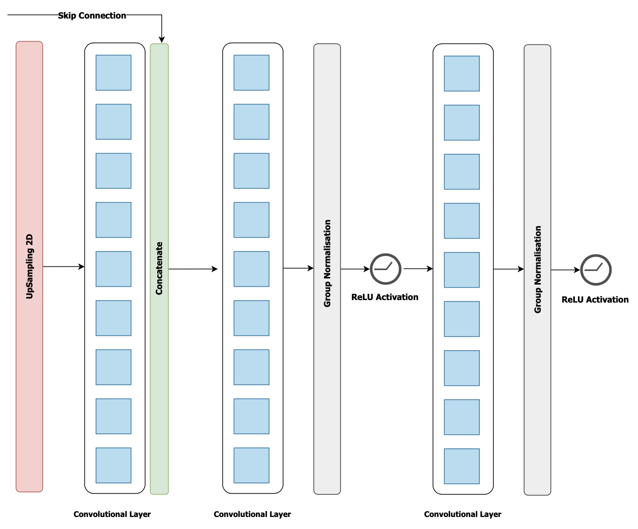
Figure 1: Deterministic UNet Decoder Block

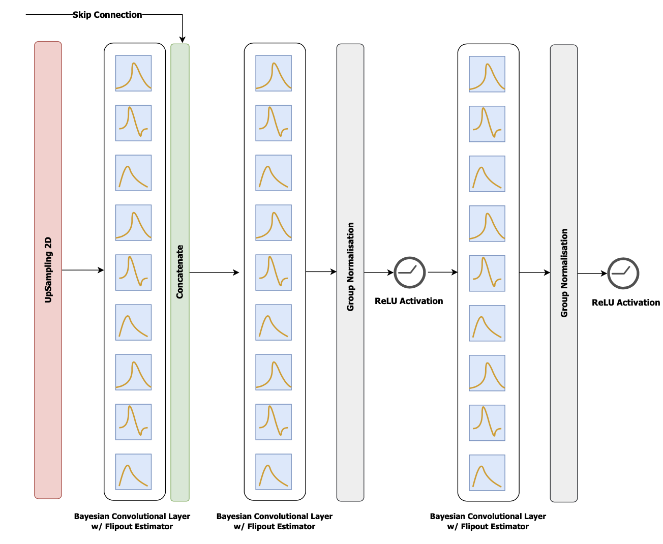
Figure 2: Bayesian UNet Decoder Block

Having established the optimal configuration of the decoder, we the investigated the impact of varying the number of filters used to initialise the model. For each stage within the encoder the number of filters doubles until the bottleneck stage is reached where the number of filters is $2^{n}$ (n - number of encoder stages) times the number of filters used in the first stage. Each stage is made up of two matched convolutional layers separated by a non-linear activation and normalisation layer. The UNET architecture proposed by [1] utilised 64 filters in the first stage leading to 1024 filters in the bottleneck. However, this would result in a model with over 50 million parameters due to the use of probabilistic layers which is too computationally expensive to train given our limited compute resources. As a result it was necessary to reduce the number of filters at each convolutional layer. Table 1 shows the performance of our model when initialising with 16 $\&$ 32 filters.

	Training Fit	F1 Score	IoU	Trainable Parameters
16	0.9908	0.836	0.741	3,181,809
32	0.9918	0.865	0.779	12,717,537

Table 1: Effect of varying filter initialisation on model accuracy and complexity

Table 1 clearly shows that despite the added computational cost of using 32 filters at initialisation, the segmentation accuracy of the model increases (3.5$\%$ increase in F1 Score and 5.1$\%$ increase in IoU). As a result, we opted to initialise our model with 32 filters and used a batch size of 32 to ensure we remain within the constraints of our available GPU RAM.

In addition to the use of Bayesian layers in the decoder, our model leverages attention mechanisms to improve the segmentation accuracy. To empirically determine the optimal configuration of attention mechanisms in our model we compared the training fit and segmentation accuracy (F1 Score $\&$ IoU) of 2 different configurations. The first configuration was consistent with [17] where we place the Convolutional Block Attention Module (CBAM) proposed by [27] in the bottleneck stage. The bottleneck stage contains the most abstract and compressed form of the input image and by applying the channel and spatial attention mechanisms the model is able to selectively focus relevant features and discern important contextual information. The second configuration aimed to build-on the advantages of including the CBAM at the bottleneck by also including the module in the final layer of the encoder (Encoder Layer 4) and first layer of the decoder (Decoder Layer 1). The rationale behind an attention mechanism in the final encoder stage was refinement of feature representations and selective emphasis of relevant features prior to entering the bottlenecks. On the other hand, including an attention mechanism in the first decoder layer may guide the network when constructing the segmentation mask and ensure that the features provided via skip connections from the encoder are attentively refined.

Location of Attention Module	Training Fit	F1 Score	IoU
Bottleneck Only	0.992	0.877	0.792
Central Layers	0.992	0.876	0.788

Table 2: Effect of varying filter initialisation on model accuracy and complexity

We can see from Table 2, that we achieved similar performance when incorporating the attention module into the central layers of our model as including it solely in the bottleneck stage. In fact, inclusion of the attention module in the bottleneck alone resulted in better accuracy on our test data. This was contrary to our initial hypothesis that the inclusion of an attention modules in additional layers would increase segmentation accuracy. A possible explanation for the slight reduction in performance is the the disruption of the feature extraction process in the bottleneck by allowing selective focusing in adjacent layers. As a result of our testing, we opted to use a single attention module located in the bottleneck which has the added benefit of reduced model complexity.

Finally, in order to improve training efficiency we included feature normalisation which maintains gradient flow during backpropogation (mitigates against vanishing $\&$ exploding gradients) and enables higher learning rates to speed up the training process. In particular, Batch Normalisation and Group Normalisation are often used for UNet-based architectures. Batch normalisation normalises the output of the activation layer by subtracting the batch mean and dividing by the batch standard deviation. However this results in a dependency on the batch size with small batch sizes resulting in noisy mean and standard deviation estimates that are not representative of the entire dataset. Group normalisation divides channels into groups and computes group-specific mean and variance and therefore is independent of the batch size. However, this results in the addition of a hyper-parameter to control the number of groups which will require tuning for a particular segmentation task. We compared the performance of both normalisation techniques and observed that Group Normalisation with a group size of 32 achieved an 8.8 $\%$ higher F1 Score and 8.2$\%$ higher IoU and as a result we opted to used Group Normalisation for our final model architecture.

Figure 3 shows the architecture of the BA U-Net incorporating all of the design choices which we have presented in this section and justified using empirical results.

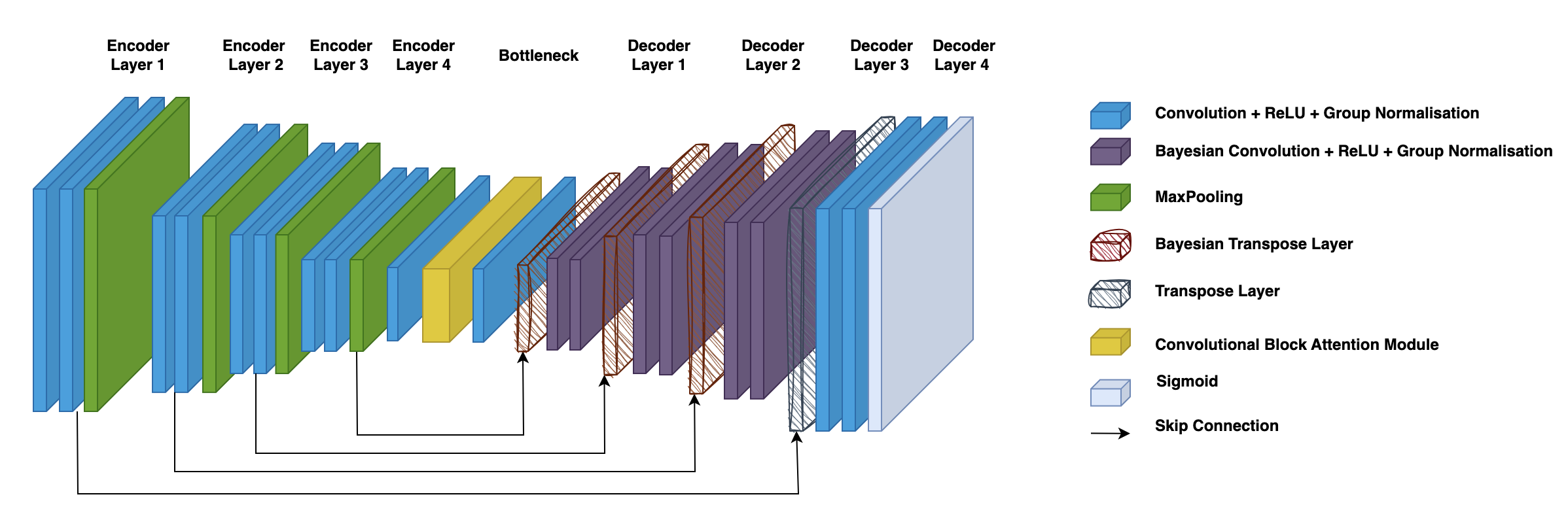
Figure 3: Architecture of Bayesian Attention U-Net

Experimental Setup

Dataset

To validate the performance our of proposed architecture we chose to use the publicly available BraTS 2020 dataset [13], [12]. The dataset consists of multi-institutional pre-operative multi-modal MRI scans that were clinically-acquired. It includes scans of glioblastoma (HGG) and lower grade glioma (LGG). The MRI data is multi-modal and contains four-types of MRI sequences: Native (T1), Post-Contrast T1-weighted, T2-weighted and T2 Fluid Attenuated Inversion Recovery (FLAIR). The BraTS 2020 dataset contains annotated multi-modal MRI data for 369 diffuse glioma patients with the ground truth tumour labels provided by expert human annotators. Each of the MRI volume is skull-stripped and co-aligned to the SRI24 anatomical atlas [30].

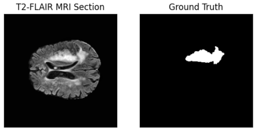
Figure 4: BraTS 2020 T2-FLAIR MRI section with ground-truth tumour annotation

In order to train our segmentation model it is necessary to process this data further and create a training, validation and test set. Our segmentation model requires 2D sections with an associated ground-truth segmentation (as shown in Figure 4). Each MRI volume contains 155 slices however slices from at the extremities of the volume are not of interest so instead we sample 100 slices from each volume to improve the data processing efficiency. As mentioned above each MRI volume contains four sequence modalities of which T2-FLAIR is optimal for visualising fluid-filled structures in the brain such as peritumoral edema. This results a clearer view of the tumor’s boundaries and surrounding affected tissue in a 2D section.

To construct our training, validation and test datasets we randomly selected 2000 MRI sections from the processed data and split this into our three datasets according to a 70:10:20 ratio. This yielded 1700 training images, 100 validation images and 200 test images each with corresponding ground-truth annotations.

Model Training

Our segmentation model was trained using the Bayes by Backprop algorithm proposed by [23] which requires the use of the variational free energy, $\mathcal{F}(\mathcal{D},\theta)$ as the loss function. However using the amendment proposed [24] we can adapt this function to be compatible with a mini-batch gradient descent scheme. Consider randomly splitting the dataset $\mathcal{D}$ into M subsets i.e. $\mathcal{D}_{1},\mathcal{D}_{2}...\mathcal{D}_{M}$, the mini-batch cost, $\mathcal{F}(\mathcal{D}_{i},\theta)$ for $i\in{1,2,...,M}$ for each epoch, E is given by:

$$\mathcal{F}^{E}(\mathcal{D}_{i},\theta)=\frac{1}{M}KL[q(\boldsymbol{w}|\theta)||p(\boldsymbol{w})]-\mathbb{E}_{q(\boldsymbol{w}|\theta)}[\log p(\mathcal{D}_{i}|\boldsymbol{w})]$$ (9)

This is clearly equivalent to the variational free energy function defined in Equation 6 as $\sum_{i=1}^{M}\mathcal{F}(\mathcal{D}_{i},\theta)=\mathcal{F}(\mathcal{D},\theta)$. [24] argues the KL divergence penalty should be distributed evenly over each mini-batch as given Equation 9 above. However, [23] propose an alternative non-linear scheme where the KL divergence scaling, $\pi_{i}$ is given by $\frac{2^{M}-i}{2^{M}-1}$. When using this scaling the first few mini-batches are influenced by the KL divergence cost and the later mini-batches are influenced by the likelihood cost.

Furthermore, the derivation of the variational free energy function, $\mathcal{F}(\mathcal{D}_{i},\theta)$ shows using this as a cost function represents a trade-off between the likelihood cost and the KL divergence penalty. The likelihood cost is a measure of well the model fits the data and therefore directly impacts the accuracy of the segmentation. On the other hand the KL divergence penalty acts as a regularisation ensuring the variational approximation to the posterior remains close to the prior distribution defined on the weights. As a result, to ensure reliable convergence of our model it is necessary to scale the KL divergence function by a factor, $\beta_{0}<1$, which allows the model to learn the segmentation without being subjected to a KL divergence regularisation that is too strong.

Incorporating these amendments gives us the final form for our variational free energy loss function:

$$\mathcal{F}^{E}(\mathcal{D}_{i},\theta)=\beta_{0}\pi_{i}KL[q(\boldsymbol{w}|\theta)||p(\boldsymbol{w})]-\mathbb{E}_{q(\boldsymbol{w}|\theta)}[\log p(\mathcal{D}_{i}|\boldsymbol{w})]$$ (10)

We opted for the Adam stochastic optimiser [31] with an intial learning rate, $\alpha=0.001$. A ReduceLROnPlateau callback was used to reduce the learning rate if the loss function plateaus for more than 10 epochs. Our model was trained on an NVIDIA A100 GPU with 40GB of VRAM provided through Google Colab. Our training images (2D MRI T2-FLAIR Sections) were re-sized to 256x256x1 with a maximum batch size of 32. The model was trained over 15 epochs and achieved a 99.2$\%$ training accuracy.

Model Inference

To obtain the mean and variance of the predictive distribution, $\mathbf{f}^{\mathbf{\widehat{W}}}(x)$, we can use Monte Carlo sampling. This is equivalent to running $T$ forward passes for the same input image and estimating the mean, $\mathbf{\hat{y}}$ and variance, $\hat{\sigma}^{2}$ from the set of output segmentation. From these estimates we can compute the aleatoric and epistemic uncertainty by utilising the predictive variance estimator derived by [2]:

$$\underbrace{\frac{1}{T}\sum_{t=1}^{T}\mathbf{\hat{y_{t}}}^{2}-\left(\frac{1}{T}\sum_{t=1}^{T}\mathbf{\hat{y_{t}}}\right)^{2}}_{\text{Aleatoric Uncertainty}}+\underbrace{\frac{1}{T}\sum_{t=1}^{T}\hat{\sigma_{t}}^{2}}_{\text{Epistemic Uncertainty}}$$ (11)

The value of $T$ used can be determined empirically by observing how the variance of the aleatoric and epistemic uncertainty estimates for validation images changes with an increasing number of MC samples. Figure 5 (below) shows the results from varying the number of MC samples from 5 to 30. It should be noted that increasing the number of MC samples increases the computational cost at inference time as a result we opted for $T=20$ which results in adequate variance reduction whilst maintaining efficiency during inference.

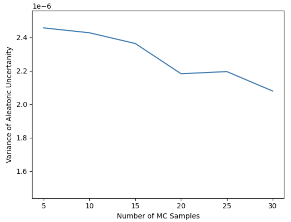
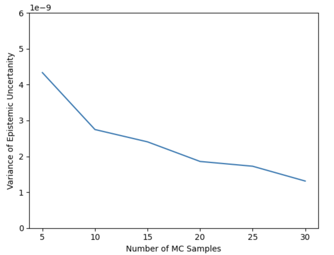
Figure 5: Variance Analysis of Aleatoric and Epistemic Uncertainties

The mean $\mathbf{\hat{y}}$ is used as the MRI segmentation and its accuracy is measured using two accuracy metrics, F1 Score and Intersection over Union (IoU). The F1 Score is the harmonic mean of precision and recall; precision is the ratio of true-positives (TP) to the all positive classifications (TP+FP) and recall is the ratio of true-positives to all known positive classifications (TP+FN).

$$F1=\frac{Precision*Recall}{Precision+Recall}=\frac{2TP}{2TP+FP+FN}$$ (12)

where $TP$ - true positive, $FP$ - false positive, $FN$ - false negative. F1 score provides a single measurement capturing both model precision and recall (sensitivity). By considering FP and FN results F1 scores are robust to imbalances in the dataset unlike simpler metrics such as binary accuracy. However, an F1 score is not robust to variations in target object size which is a key feature of medical images as a result we opted to use an additional accuracy metric - Intersection over Union (IoU). IoU is the ratio of the area of intersection to the area of the union; the intersection area is the where the predicted bounding box overlaps with the ground-truth and the union area is the total area covered by both the predicted bounding box and ground-truth.

$$IoU=\frac{Intersection}{Union}=\frac{|A\cap B|}{|A\cup B|}$$ (13)

The IoU provides a quantitative measure of a model’s ability to localise and object within an image and is robust to variations in object size. IoU is also well-suited to scenes where objects may be occluded. By leveraging the merits of two accuracy metrics we are able to obtain a more complete understanding of our model’s classification and localisation performance.

Having obtained estimates of the $\mathbf{\hat{y}}$ and variance, $\hat{\sigma}^{2}$ via Monte Carlo sampling we can use the formulation proposed by [2] to generate 2D maps of the aleatoric and epistemic uncertainty. We can calculate the mean of these 2D uncertainty maps to get an estimate for the average aleatoric and epistemic uncertainty in the segmentation of a given image. Combining the average aleatoric and epistemic uncertainties gives us an estimate for the overall predictive variance in the final segmentation as shown in Equation 2. To test the applicability of our uncertainty estimates we compare the estimate for a clear MRI with one that have been progressively degraded to determine whether the uncertainty estimates provided by the model are sensitive to such changes. We can then empirically obtain an uncertainty threshold to effectively incorporate human in-the-loop decision making [3].

Results

In this section we present the inference results of our BA U-Net segmentation model on the BraTS 2020 dataset. We include the the predicted segmentation and a visualisation of the aleatoric and epistemic uncertainty.

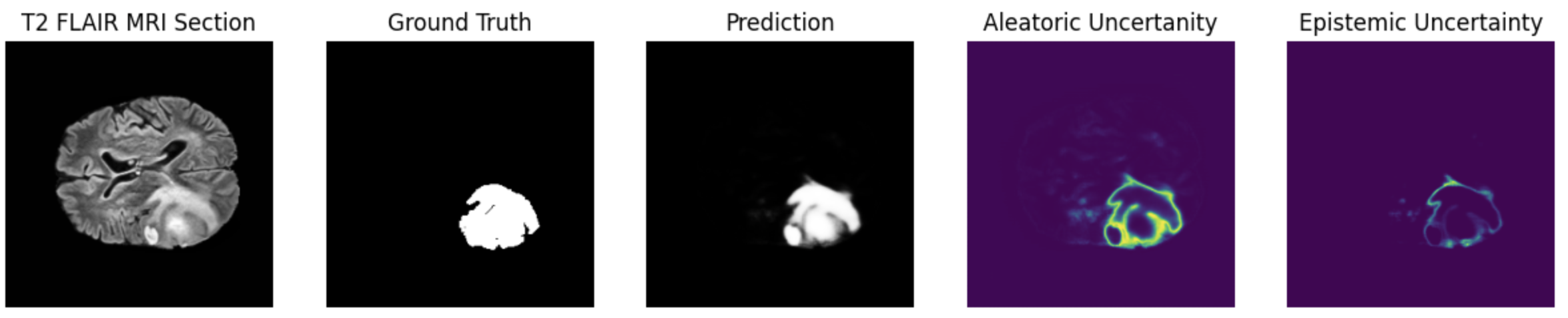
(a) F1 Score: 0.924, IoU: 0.860

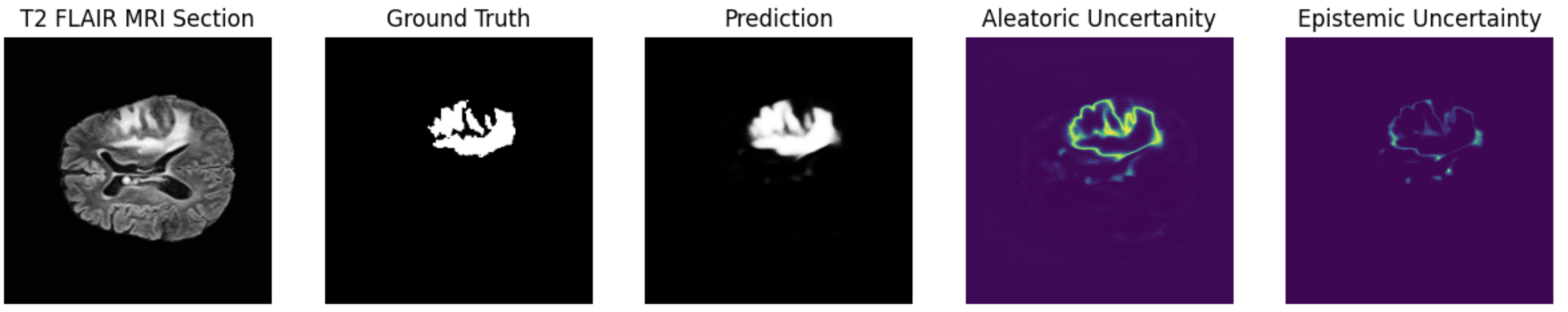
(b) F1 Score: 0.947, IoU: 0.899

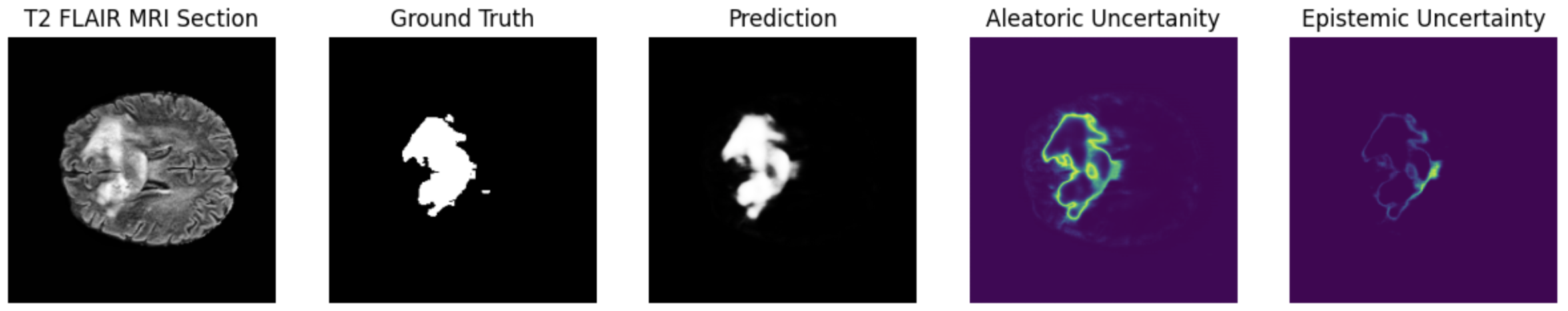
(c) F1 Score: 0.905, IoU:0.827

Figure 6: BA U-Net Inference on BraTS 2020 Dataset

Our test dataset contained 314 images and we achieved an average F1 Score: 0.877 and an IoU: 0.792. This represents an improvement over existing variational approaches to MRI image segmentation [11] and is competitive when compared with submissions to the BraTS 2020 Competition. For each segmentation we were able to estimate the aleatoric and epistemic uncertainty however validation of these uncertainties is challenging due to the lack of standardised benchmarks.

As a result, we opted to test the performs of our approach on progressively degraded MRIs paying close attention to the response of the overall model uncertainty (aleatoric + epistemic). We measured the response to three types of image degradation: Gaussian Blur, Rician Noise and Brightness/Contrast Changes. These were chosen on the basis they best reflect the alterations that are commonly found in real-world medical image data.

Gaussian Blur

$$G_{\sigma}(x,y)=\frac{1}{2\pi\sigma^{2}}exp(-\frac{x^{2}+y^{2}}{2\sigma^{2}})$$ (14)

Equation 14 is a 2D Gaussian kernel and we apply this function to our MRI image prior to inference using our uncertainty-aware model. Figure 7 below shows our results for $\sigma=2.6$ and $\sigma=4.4$.

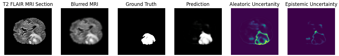
(a) $\sigma=2.6$ - $5.1\%$ Increase in Model Uncertainty

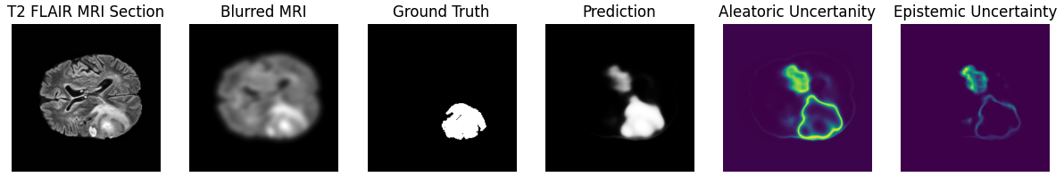
(b) $\sigma=4.4$ - $60.9\%$ Increase in Model Uncertanity

Figure 7: Inference on Gaussian Blur Degraded MRI Section

Rician Noise

The noise present in magnitude MRI images has been shown to be governed by a Rician distribution [32]. A Rician distribution can be approximated using the Rayleigh distribution in regions where there is no NMR signal. As a result, we apply noise governed by this Rayleigh distribution.

$$f(x;\sigma)=\frac{x}{\sigma^{2}}e^{-x^{2}/(2\sigma^{2})},\quad x\geq 0$$ (15)

where $\sigma$ is the scale parameter of the distribution. The Rayleigh distribution is the magnitude of a two-dimensional vector whose components are independent Gaussian random variables with equal variances and zero means. If $X$ and $Y$ are such Gaussian random variables, then the random variable representing their magnitude, $Z$ will be Rayleigh distributed.

$$Z=\sqrt{X^{2}+Y^{2}}\hskip 10.00002ptwhere\hskip 10.00002ptX\sim\mathcal{N}(0,\sigma^{2}),\quad Y\sim\mathcal{N}(0,\sigma^{2})$$ (16)

Figure 8 below shows our results for $\sigma=0.3$

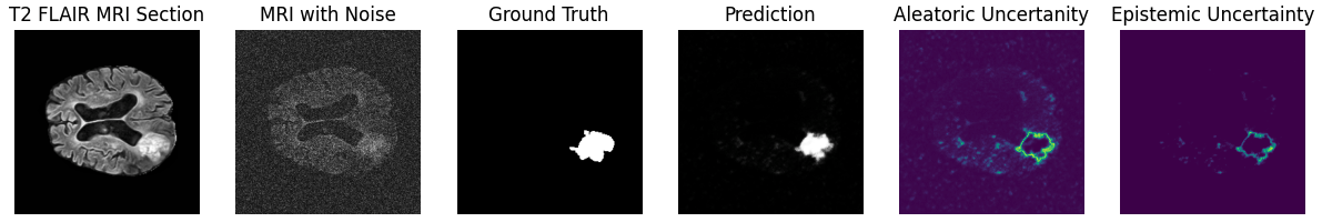
(a) 21.5$\%$ Increase in Model Uncertainty

Figure 8: Inference on Rician Noise Degraded MRI Section

Brightness $\&$ Contrast

The final degradation we performed on the MRI test data was applying a random brightness and contrast change to the MRI image and observing the response in model uncertainty. Figure 9 shows the results of an image with reduced brightness and contrast. The brightness of each pixel was reduced by 50 and each pixel value was scaled by a contrast factor of 0.8.

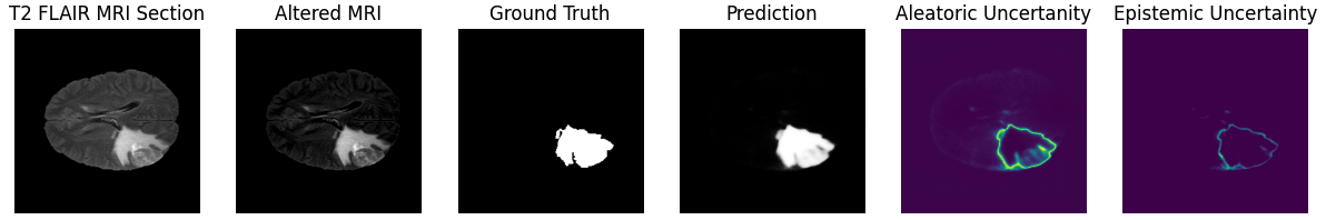
(b) 5.7$\%$ Increase in Model Uncertainty

Figure 9: Inference on Brightness $\&$ Contrast Degraded MRI Section

Discussion

The results shown in the previous section were obtained by running 20 stochastic forward passes on a randomly chosen test image with the prediction mean representing the segmentation and the model uncertainty obtained using the formula outlines in Equation (2). The model uncertainty can expressed as the sum of the aleatoric and epistemic uncertainties. As outlined previously, the aleatoric uncertainty is a measure of the uncertainty due to the inherent variability in the data and epistemic uncertainty is a measure of the uncertainty due to limitations of our model. Figure 6 shows the results on clean processed MRI sections with visualisations of the two respective uncertainty components. Here we can see that the model is confident in its predicted segmentation with the high intensity regions being concentrated at the boundaries of the segmented area indicating reduced confidence on the boundaries of the tumour. Even for clear MRI scans this provides a level of interpretability that would be otherwise unavailable in a purely deterministic model. In Figure 6 a) we can observe that despite the very high F1 Score (0.924) that the model was unsure about the presence of a sub-structure within the tumour and this is highlighted in the visualisation of the aleatoric uncertainty.

To further demonstrate the capabilities of our BA U-Net we chose to test the inference capabilities of our model on degraded MRI scans. We chose three types of image degradation - Gaussian Blur, Rician Noise and Brightness/Contrast Changes. We argue that these are indicative of the types of degradation that are present in real-world MRI data and the true applicability of our approach would be contingent on a demonstrable increase in model uncertainty (aleatoric + epistemic) in such cases. Figure 7 shows the results of running inference on Gaussian Blur degraded MRI sections for two different values of standard-deviation, $\sigma$. For $\sigma=2.6$ (see Figure 7a), we observe that there only a slight effect on image quality and this is reflected in the marginal increase in model uncertainty. From the visualisation of the respective uncertainty we can observe that this increase is due to model being uncertain of the presence of a second structure within the MRI as indicated by the highlighted regions away from the main tumour boundary. This gives a precise understanding of the effect of a weak Gaussian blur on an MRI image and the segmentation errors it can cause. Figure 7b) shows the results from using a higher value of $\sigma=4.4$., here there was a significant increase in model uncertainty of $61\%$ which is consistent with the significant blurring of the image. We can also observe that the predicted segmentation now contains an erroneous second tumour however on consulting the visualisations of uncertainty we can see that the model is highly uncertain regarding this prediction as emphasised by the highlighted pixels both on the border and inside of the predicted region.

Following the application of a Gaussian Blur, we chose to apply an approximation of Rician noise and obtain our model’s response to this form of image degradation. We chose Rician noise as [32] argue that it is the governing distribution of noise is magnitude MRI images such as the ones we used to test our model. Figure 8 shows we observe a $21.5\%$ increase in model uncertainty when performing inference on a noisy MRI image. We can observe from the visualisations of the uncertainty that the presence of noise interfered with model confidence in regions where it would have otherwise been highly confident for a clean MRI image.

Our final degradation modality was altering the brightness and contrast profile of our MRI images. Figure 9 shows that we the altered MRI has undergone a significant brightness reduction and contrast reductions testing the model’s ability to ascertain tumour boundaries. We observe a $5.7\%$ increase in model uncertainty with the visualisation showing increased uncertainty around the boundaries of the tumour likely as expected.

Conclusion

Im summary, we present an uncertainty aware segmentation model, BA U-Net and evaluate its performance on the whole tumour (WT) segmentation task in the BraTS 2020 dataset. We obtain an F1 Score of 0.877 and IoU of 0.792. This is an improvement over previous variational approaches [11] and is competitive amongst models submitted as part of the BraTS 2020 challenge. However, the clear advantage of our approach is it ability to provide credible estimates of model uncertainty which we validated empirically by running inference on degraded MRI images. By applying systematic degradation of the MRI we are attempting to mimic the effect of real-world MRI data where the presence of image artifacts could result in a faulty segmentation where the model incorrectly classifies regions within an image. Our results clearly show that for each image degradation type the BA U-Net reports an increase in its uncertainty metric which correlates with the extent of image degradation. Moreover, the aleatoric and epistemic uncertainty can be visualised to show the regions of the predicted segmentation where the model is not confident. Typically this will be around the borders of the segmentation however we observed interesting effects when the MRI image is significantly affected by image degradation where the model may misidentify additional tumours in the MRI scan and by observing the uncertainty map we can determine how confident the model is in this prediction. Overall, our model is able to provide highly accurate whole tumour (WT) segmentations on MRI data and provide credible uncertainty estimates which have been shown to be responsive to artifacts present in real MRI image data.

References

- [1] Olaf Ronneberger, Philipp Fischer and Thomas Brox “U-Net: Convolutional Networks for Biomedical Image Segmentation” In Medical Image Computing and Computer-Assisted Intervention – MICCAI 2015 Cham: Springer International Publishing, 2015, pp. 234–241
- [2] Alex Kendall and Yarin Gal “What uncertainties do we need in bayesian deep learning for computer vision?” In Advances in neural information processing systems 30, 2017
- [3] Nabeel Seedat “MCU-Net: A framework towards uncertainty representations for decision support system patient referrals in healthcare contexts” In CoRR abs/2007.03995, 2020 arXiv: https://arxiv.org/abs/2007.03995
- [4] Christopher M. Bishop “Pattern Recognition and Machine Learning (Information Science and Statistics)” Berlin, Heidelberg: Springer-Verlag, 2006
- [5] Balaji Lakshminarayanan, Alexander Pritzel and Charles Blundell “Simple and scalable predictive uncertainty estimation using deep ensembles” In Advances in neural information processing systems 30, 2017
- [6] Yarin Gal and Zoubin Ghahramani “Dropout as a bayesian approximation: Representing model uncertainty in deep learning” In international conference on machine learning, 2016, pp. 1050–1059 PMLR
- [7] Nitish Srivastava et al. “Dropout: a simple way to prevent neural networks from overfitting” In The journal of machine learning research 15.1 JMLR. org, 2014, pp. 1929–1958
- [8] Ian Osband “Risk versus uncertainty in deep learning: Bayes, bootstrap and the dangers of dropout” In NIPS workshop on bayesian deep learning 192, 2016
- [9] Loic Le Folgoc et al. “Is MC Dropout Bayesian?” In arXiv preprint arXiv:2110.04286, 2021
- [10] Dustin Tran, Mike Dusenberry, Mark Van Der Wilk and Danijar Hafner “Bayesian layers: A module for neural network uncertainty” In Advances in neural information processing systems 32, 2019
- [11] Abhinav Sagar “Uncertainty Quantification using Variational Inference for Biomedical Image Segmentation”, 2021 arXiv:2008.07588 [eess.IV]
- [12] Bjoern H. Menze et al. “The Multimodal Brain Tumor Image Segmentation Benchmark (BRATS)” In IEEE Transactions on Medical Imaging 34.10, 2015, pp. 1993–2024 DOI: 10.1109/TMI.2014.2377694
- [13] Spyridon Bakas et al. “Identifying the Best Machine Learning Algorithms for Brain Tumor Segmentation, Progression Assessment, and Overall Survival Prediction in the BRATS Challenge”, 2019 arXiv:1811.02629 [cs.CV]
- [14] Jonathan Long, Evan Shelhamer and Trevor Darrell “Fully Convolutional Networks for Semantic Segmentation” In Proceedings of the IEEE Conference on Computer Vision and Pattern Recognition (CVPR), 2015
- [15] Ozan Oktay et al. “Attention u-net: Learning where to look for the pancreas” In arXiv preprint arXiv:1804.03999, 2018
- [16] Sanghyun Woo, Jongchan Park, Joon-Young Lee and In So Kweon “CBAM: Convolutional Block Attention Module” In Proceedings of the European Conference on Computer Vision (ECCV), 2018
- [17] Changlu Guo et al. “Sa-unet: Spatial attention u-net for retinal vessel segmentation” In 2020 25th international conference on pattern recognition (ICPR), 2021, pp. 1236–1242 IEEE
- [18] Yarin Gal and Zoubin Ghahramani “Bayesian convolutional neural networks with Bernoulli approximate variational inference” In arXiv preprint arXiv:1506.02158, 2015
- [19] Tyler J Loftus et al. “Uncertainty-aware deep learning in healthcare: a scoping review” In PLOS digital health 1.8 Public Library of Science San Francisco, CA USA, 2022, pp. e0000085
- [20] Golnaz Ghiasi, Tsung-Yi Lin and Quoc V Le “Dropblock: A regularization method for convolutional networks” In Advances in neural information processing systems 31, 2018
- [21] Sai Harsha Yelleni, Kumari Deepshikha, PK Srijith and C Krishna Mohan “Monte Carlo DropBlock for modelling uncertainty in object detection” In Pattern Recognition Elsevier, 2023, pp. 110003
- [22] Francesco Verdoja and Ville Kyrki “Notes on the behavior of mc dropout” In arXiv preprint arXiv:2008.02627, 2020
- [23] Charles Blundell, Julien Cornebise, Koray Kavukcuoglu and Daan Wierstra “Weight uncertainty in neural network” In International conference on machine learning, 2015, pp. 1613–1622 PMLR
- [24] Alex Graves “Practical variational inference for neural networks” In Advances in neural information processing systems 24, 2011
- [25] Kingma and Welling “Auto-encoding variational bayes” In arXiv preprint arXiv:1312.6114, 2013
- [26] Durk P Kingma, Tim Salimans and Max Welling “Variational dropout and the local reparameterization trick” In Advances in neural information processing systems 28, 2015
- [27] Yeming Wen et al. “Flipout: Efficient Pseudo-Independent Weight Perturbations on Mini-Batches” In CoRR abs/1803.04386, 2018 arXiv: http://arxiv.org/abs/1803.04386
- [28] Reza Azad, Maryam Asadi-Aghbolaghi, Mahmood Fathy and Sergio Escalera “Bi-directional ConvLSTM U-Net with densley connected convolutions” In Proceedings of the IEEE/CVF international conference on computer vision workshops, 2019, pp. 0–0
- [29] Joshua V Dillon et al. “Tensorflow distributions” In arXiv preprint arXiv:1711.10604, 2017
- [30] Torsten Rohlfing, Natalie M Zahr, Edith V Sullivan and Adolf Pfefferbaum “The SRI24 multichannel atlas of normal adult human brain structure” In Human brain mapping 31.5 Wiley Online Library, 2010, pp. 798–819
- [31] Kingma and Ba “Adam: A method for stochastic optimization” In arXiv preprint arXiv:1412.6980, 2014
- [32] H. Gudbjartsson and S. Patz “The Rician distribution of noisy MRI data” In Magn Reson Med 34.6, 1995, pp. 910–914