Fast Estimation of the Renshaw-Haberman Model and Its Variants

Abstract

In mortality modelling, cohort effects are often taken into consideration as they add insights about variations in mortality across different generations. Statistically speaking, models such as the Renshaw-Haberman model may provide a better fit to historical data compared to their counterparts that incorporate no cohort effects. However, when such models are estimated using an iterative maximum likelihood method in which parameters are updated one at a time, convergence is typically slow and may not even be reached within a reasonably established maximum number of iterations. Among others, the slow convergence problem hinders the study of parameter uncertainty through bootstrapping methods.

In this paper, we propose an intuitive estimation method that minimizes the sum of squared errors between actual and fitted log central death rates. The complications arising from the incorporation of cohort effects are overcome by formulating part of the optimization as a principal component analysis with missing values. We also show how the proposed method can be generalized to variants of the Renshaw-Haberman model with further computational improvement, either with a simplified model structure or an additional constraint. Using mortality data from the Human Mortality Database (HMD), we demonstrate that our proposed method produces satisfactory estimation results and is significantly more efficient compared to the traditional likelihood-based approach.

Keywords: Cohort effects; Missing values; Principal component analysis; The Renshaw-Haberman model

1 Introduction

Research in mortality modelling has grown significantly over the past several decades, largely due to its substantial implications in actuarial science, demography, and public health. A fundamental concept in this field is cohort effects, which describe the unique mortality influences experienced by groups born in the same time period, for example, the year of birth. The study of cohort effects has a long history, for example, Hobcraft et al. (1982) and Wilmoth (1990) and it has been recognized as a pivotal element in predicting mortality rates and managing longevity risks. Cohort effects are highly country or region specific, and it is widely acknowledged that the effects have been most outstanding in the United Kingdom. Several studies, for example, Willets (2004), revealed the so-called “golden generation” for those who were born in the UK around the early 1930s and have had significantly high mortality rate improvements. For certain countries or regions with notable cohort effects, it can significantly influence the mortality forecasts and as a result, the financial sustainability of insurance and pension systems.

The Renshaw-Haberman model, proposed by Renshaw and Haberman (2006), represents a significant milestone in the research of mortality studies, building on the seminal Lee-Carter model (Lee and Carter, 1992). Despite recent discoveries of potential inference pitfalls (Leng and Peng, 2016; Liu et al., 2019), the Lee-Carter model remains a significant and widely adopted stochastic mortality model in both academia and insurance practice. The Renshaw-Haberman model extends the Lee-Carter model by incorporating an age-specific time-varying cohort effect and establishes a connection to the age-period-cohort (APC) model, a more traditional mortality model involving cohort effects in demography (Hobcraft et al., 1982). This integration of the cohort effect has enhanced the model’s ability to represent complex mortality dynamics and improved its predictive accuracy. Recent extensions of the Renshaw-Haberman model have further addressed specific features of mortality data, such as socioeconomic disparities (Villegas and Haberman, 2014), and allowed for its application in more general actuarial and insurance contexts.

The estimation of the parameters in the Renshaw-Haberman model is traditionally MLE-based. More precisely, it adopts an iterative Newton-Raphson method to seek a maximum likelihood estimate (MLE) under the framework of Poisson generalized linear models (GLM). However, the parameter estimation procedure has long been known to present challenges, with notable issues of slow convergence and stability, as noted by for example, Cairns et al. (2009, 2011), Haberman and Renshaw (2009, 2011). One plausible cause for this slow convergence is the nature of the log-likelihood or deviance function. Specifically, these functions tend to be almost flat when approaching their optimal points. This flatness, which intensifies the convergence issue, is primarily a result of the expansive, high-dimensional parameter space emerging from overparameterization in the model.

The slow convergence and computational challenges in the Renshaw-Haberman model significantly restrict its application in mortality forecasting and actuarial science. Firstly, these issues hinder the use of bootstrapping, a widely adopted method for assessing uncertainties in stochastic mortality models (Koissi et al., 2006). Given the iterative nature of bootstrapping resampling, slow convergence of the model directly causes computational inefficiencies and limits its practical utility. Secondly, the computational challenges present barriers to further model extensions, such as multi-population models and enhancements with additional cohort effect terms. These extensions inherently require more computational power, which is already strained by the existing estimation process in the original Renshaw-Haberman model. Lastly, computational difficulties can also impact the practicality of the model, particularly in a field where timely data analysis and prediction are critical, such as insurance or pension fund management. These issues could lead to outdated forecasts when dealing with large datasets, potentially affecting financial decision-making and risk management strategies. Hence, overcoming these challenges is crucial for the wider and more efficient application of the Renshaw-Haberman model.

To address computational challenges in the Renshaw-Haberman model, Renshaw and Haberman (2006) proposed several sub-models with a reduced number of parameters, including the APC model, to relax the computational burden associated with the full model. Hunt and Villegas (2015) subsequently identified an approximate identification issue in the Renshaw-Haberman model, recommending an additional constraint to stabilize the estimation process and enhance algorithmic robustness. These advancements primarily concentrate on improving computation speed and stability by constraining the parameter space, achieved either through parameter reduction or imposing additional constraints.

In this paper, we explore an alternative approach to improving the computational efficiency of the Renshaw-Haberman model. To the best of our knowledge, all existing methods for parameter estimation in this model are predicated on an MLE framework, seeking to maximize the log-likelihood of a Poisson generalized linear model (GLM). However, the seminal Lee-Carter model, a precursor to the Renshaw-Haberman model, originally employed a least squares estimation method for parameter estimation (Lee and Carter, 1992), with the MLE approach introduced later by Brouhns et al. (2002). This observation raises a natural question: why has the least squares approach not been explored for the Renshaw-Haberman model? The least squares method offers several advantages over MLE, notably its independence from distributional assumptions of the mortality data and, in certain scenarios (e.g., the closed-form solution for the Lee-Carter model), enhanced computational efficiency.

We propose an intuitive “least-square type” estimation method for the Renshaw-Haberman model, drawing inspiration from the singular value decomposition (SVD) technique utilized in the Lee-Carter model. Our method seeks to directly minimize the squared error between actual and estimated log central mortality rates. We address the technical challenges posed by cohort effects through an alternating minimization strategy, reformulating a part of the optimization as a Principal Component Analysis (PCA) with missing values. This component can be efficiently resolved using an iterative SVD algorithm, for which we provide theoretical validation. Our empirical analyses, employing mortality data from the Human Mortality Database (HMD), demonstrate the reliability and computational superiority of our method compared to traditional MLE approaches. Furthermore, we explore the applicability of our least squares estimation technique to variants of the Renshaw-Haberman model. We particularly focus on the H1 model, where the age effect in cohort trends is constant. In this case, we also demonstrate how the additional constraint suggested by Hunt and Villegas (2015) can be integrated into our method.

The remainder of this paper is organized as follows. Section 2 presents an overview of the Lee-Carter model, including both the least squares and MLE-based estimation methods. In Section 3, we review the Renshaw-Haberman model, discussing its well-recognized estimation challenges and the motivations underpinning our study. Section 4 details our primary contribution, a least square parameter estimation approach for the Renshaw-Haberman model and its variants. Section 5 elaborates on the extension of our method to the H1 model and the integration of additional constraints. Section 6 is dedicated to validating our approach and demonstrating its computational efficiency through a series of numerical experiments. Finally, we conclude this paper and make remarks for future research in Section 7.

2 The Lee-Carter Model

This section presents a concise background to the Lee-Carter model, with a main focus on parameter estimation. We also discuss the difference of the MLE-based and least square methods, which is essential for our primary discussion on the Renshaw-Haberman model.

The Lee-Carter model, first proposed by Lee and Carter (1992), provides a simple bilinear form to represent the log central mortality rate as follows:

$$y_{x,t}:=\log(m_{x,t})=a_{x}+b_{x}k_{t}+\varepsilon_{x,t},$$ (2.1)

Here, $m_{x,t}$ denotes the central mortality rate for age $x$ in year $t$, and for the sake of notational simplicity, we denote $y_{x,t}:=\log(m_{x,t})$. The data used for mortality calculations span across $p$ different ages $x\in[x_{1},\cdots,x_{p}]$ and $n$ calendar years $t\in[t_{1},\cdots,t_{n}]$.

Within the Lee-Carter model (2.1), there is a deterministic part, $a_{x}+b_{x}k_{t}$, and a stochastic error term, $\varepsilon_{x,t}$. The deterministic part, or the estimate $\hat{y}_{x,t}$ of the true log mortality rate $y_{x,t}$, is where $a_{x}$ depicts the shape of log mortality rates across ages, $k_{t}$ indicates the overall mortality trend across time, and $b_{x}$ adjusts the trend of $k_{t}$ in relation to ages. To guarantee that the parameters are uniquely identified, Lee and Carter (1992) impose two constraints:

$$\sum_{x=x_{1}}^{x_{p}}b_{x}=1\quad\text{and}\quad\sum_{t=t_{1}}^{t_{n}}k_{t}=0.$$ (2.2)

The original method to estimate the parameters of the Lee-Carter model, proposed by Lee and Carter (1992), follows the least squares principle and does not rely on any distributional assumptions. This solution minimizes the total square error between the observed and the fitted log central mortality rates $y_{x,t}$. For clarity, we can rewrite the Lee-Carter model in vector form. Denoting $\bm{y}_{t}=(y_{x_{1},t},\cdots,y_{x_{p},t})^{T}$, $\bm{a}=(a_{x_{1}},\cdots,a_{x_{p}})^{T}$, $\bm{b}=(b_{x_{1}},\cdots,b_{x_{p}})^{T}$, $\bm{k}=(k_{t_{1}},\cdots,k_{t_{n}})^{T}$, and $\bm{\varepsilon}_{t}=(\varepsilon_{x_{1},t},\cdots,\varepsilon_{x_{p},t})^{T}$, then the estimates of $\bm{a}$, $\bm{b}$ and $k_{t}$ can be obtained by solving the following least squares optimization problem:

$$\min_{\bm{a},\bm{b},\bm{k}}\sum_{x,t}(y_{x,t}-(a_{x}+b_{x}k_{t}))^{2}=\min_{\bm{a},\bm{b},\bm{k}}\sum_{t}\|\bm{y}_{t}-(\bm{a}+\bm{b}k_{t})\|_{2}^{2},$$ (2.3)

where $\|\cdot\|_{2}$ denotes the Euclidean norm (or $L^{2}$-norm) of a vector. Under the identification constraints (2.2), the optimization problem (2.3) is equivalent to a special case of PCA with the number of principal components set to one. Its optimal solution can be obtained by performing SVD on the centered log mortality data matrix $\bm{Y}-\bar{\bm{Y}}:=(\bm{y}_{t_{1}}-\bar{\bm{y}},\cdots,\bm{y}_{t_{n}}-\bar{\bm{y}})$, where $\bar{\bm{Y}}=(\bar{\bm{y}},\cdots,\bar{\bm{y}})$ and $\bar{\bm{y}}=\frac{1}{n}\sum_{t=t_{1}}^{t_{n}}\bm{y}_{t}$. Letting $\bm{u}$ be the first left-singular vector of $\bm{Y}-\bar{\bm{Y}}$, the solution of (2.3) has the following closed form:

$$\hat{\bm{a}}=\bar{\bm{y}},\quad\hat{\bm{b}}=\frac{\bm{u}}{\mathbf{1}^{T}\bm{u}},\quad\hat{\bm{k}}=(\mathbf{1}^{T}\bm{u})\cdot(\bm{Y}-\bar{\bm{Y}})^{T}\bm{u}.$$ (2.4)

In this solution, the term $\bm{1}^{T}\bm{u}$ normalizes the standard PCA solution due to the imposed constraint $\sum_{x}b_{x}=1$, where $\mathbf{1}=(1,\cdots,1)^{T}$. Additionally, it is easy to check that the constraint $\sum_{t}k_{t}=0$ is also met.

In contrast to least squares method, which does not make assumptions about the underlying distribution of mortality rates, MLE-based methods assume that the actual deaths follow a certain distribution, with model parameters embedded into the regression model. Let us denote the number of deaths and the exposure to risk for the age group $x$ at time $t$ as $D_{x,t}$ and $N_{x,t}$, respectively. The traditional Poisson GLM formulation of the Lee-Carter model, proposed by Brouhns et al. (2002), can be written as:

$$D_{x,t}\sim\text{Poisson}(N_{x,t}m_{x,t}),\text{ with }\log(m_{x,t})=a_{x}+b_{x}k_{t}.$$ (2.5)

The parameter estimation under this framework is done via MLE, that finds $a_{x},b_{x},k_{t}$ to maximize the following log-likelihood function:

$$\ell(\bm{a},\bm{b},\bm{k})=\sum_{x,t}\left(D_{x,t}(a_{x}+b_{x}k_{t})-N_{x,t}e^{a_{x}+b_{x}k_{t}}\right)+\text{const}.$$ (2.6)

The optimization problem is solved via an iterative Newton-Raphson method originally proposed by Goodman (1979), which updates each parameter in an iterative manner.

To summarize, there are two primary classes of parameter estimation methods for the Lee-Carter model:

1. Least Squares: This involves using SVD to find the least squares solution, which is the most classical method suggested by Lee and Carter (1992).

2. MLE: This involves fitting a GLM to find the maximum likelihood solution, with the most prominent method being the Poisson GLM, as proposed by Brouhns et al. (2002).

Both the least squares and MLE methods can be used to fit the Lee-Carter model, each presenting distinct features.

3 The Renshaw-Haberman Model and Its Variants

In this paper, we study the Renshaw-Haberman model, proposed by Renshaw and Haberman (2006), which extends the seminal Lee-Carter model (2.1) by incorporating an additional age-cohort interaction term to capture the cohort effect:

$$y_{x,t}:=\log(m_{x,t})=a_{x}+b_{x}k_{t}+c_{x}\gamma_{t-x}+\varepsilon_{x,t},$$ (3.1)

where $s=t-x\in[t_{1}-x_{p},t_{n}-x_{1}]$ denotes the cohort year with range $n+p-1$.

For the same reason as the Lee-Carter model, the Renshaw-Haberman model also suffers from identification issues, that can be resolved by imposing two constraints on $c_{x}$ and $\gamma_{t-x}$ in additional to (2.2):

$$\sum_{x=x_{1}}^{x_{p}}c_{x}=1,\quad\sum_{t-x=t_{1}-x_{p}}^{t_{n}-x_{1}}\gamma_{t-x}=0.$$ (3.2)

It is worth noting that the choice of the constraint for $\gamma_{t-x}$ is not unique. Another possible choice that appears in the seminal paper Renshaw and Haberman (2006) is to restrict the first value of $\gamma_{t-x}$ to be zero, that is, $\gamma_{t_{1}-x_{p}}=0$. In this paper, we choose the constraint $\sum_{t-x=t_{1}-x_{p}}^{t_{n}-x_{1}}\gamma_{t-x}=0$ which is also commonly adopted, for example Cairns et al. (2009) and the StMoMo package in R (Villegas et al., 2015). The actual choice of the constraints makes no difference to the goodness of fit.

Estimating the parameters for the Renshaw-Haberman model is well-known to be challenging. A common approach, adopted by Cairns et al. (2009) and the StMoMo package in R, entails optimizing the following log-likelihood function of the Poisson GLM:

$$\ell(\bm{a},\bm{b},\bm{k},\bm{c},\bm{\gamma})=\sum_{x,t}\left(D_{x,t}(a_{x}+b_{x}k_{t}+c_{x}\gamma_{t-x})-N_{x,t}e^{a_{x}+b_{x}k_{t}+c_{x}\gamma_{t-x}}\right)+\text{const}.$$ (3.3)

The MLE is found via an iterative Newton-Raphson procedure in which at each iteration only one parameter is updated while fixing others. The iteration cycle will stop when the log-likelihood converges. Currie (2016) explored the computational issues when fitting the model using the gnm package in R, a standard tool for fitting generalized non-linear models. He also emphasized the importance of appropriate starting values for improving convergence and suggested to use the estimates from the Lee-Carter model as the starting values.

The estimating method discussed above has come in for criticism for the slow convergence speed of the iterative procedure, as reported by much literature, for example, Cairns et al. (2009, 2011), Haberman and Renshaw (2009, 2011). To address this issue, research has focused on reducing the parameter space. One strategy is to consider simpler model structures, for example, the two sub-models proposed by Renshaw and Haberman (2006):

$$y_{x,t}:=\log(m_{x,t})=a_{x}+b_{x}k_{t}+\frac{1}{p}\gamma_{t-x}+\varepsilon_{x,t},$$ (3.4)

$$y_{x,t}:=\log(m_{x,t})=a_{x}+\frac{1}{p}k_{t}+\frac{1}{p}\gamma_{t-x}+\varepsilon_{x,t},$$ (3.5)

where $p$ is the length of the age band. The first variant (3.4) simplifies the Renshaw-Haberman model by setting $c_{x}=1/p$. This simplified model, often referred to as the H1 model, is discussed in detail by Renshaw and Haberman (2006) and Haberman and Renshaw (2011). The second variant (3.5) is achieved by setting both $b_{x}=c_{x}=1/p$. This model is commonly known as the age-period-cohort (APC) model and was first presented by Hobcraft et al. (1982). Despite the computational improvements due to these simplifications, such models may compromise the goodness of fit thus are not suggested in practice.

Another strategy to enhance computational efficiency is the introduction of additional constraints. Hunt and Villegas (2015) identified an approximate identification issue in the Renshaw-Haberman model and proposed a constraint to accelerate convergence. Section 5 will further discuss this approach and its integration into our proposed method.

Both strategies to mitigate computational challenges are both based on the MLE method, that find the parameter estimates within a reduced space to maximize certain log-likelihood functions. However, the Lee-Carter model demonstrates the potential of the least squares approach, notably its computational efficiency due to the closed-form SVD solution. This observation motivates the exploration of a least squares method for the Renshaw-Haberman model, potentially offering the following advantages:

• Objective function and computation: The two methods differ fundamentally in their objective functions, affecting the computational efficiency. The distinct objective function in the least squares method could potentially offers a computational advantage, as observed from the close-form SVD solution of the Lee-Carter model. Section 6 will empirically demonstrate this advantage, showing that the least squares method tends to have a sharper objective function compared to MLE (3.3), leading to faster convergence.

• Distributional Assumptions: The least squares approach, in contrast to the MLE method, offers a substantial advantage in terms of its independence from distributional assumptions. The MLE methods, such as Poisson GLM, require data to follow specific distributions, typically Poisson, binomial or negative binomial, leading to potential model misspecification. In contrast, the least squares method circumvents this by directly minimizing the squared differences between observed and predicted log mortality rates. This approach provides significant flexibility, allowing a broader range of data distributions and enhancing robustness in cases where mortality data deviates from specific probabilistic structure.

• Integration with current approaches: The least squares method is not mutually exclusive with other approaches aimed at enhancing the computation of the Renshaw-Haberman model. It can be naturally applied to simpler sub-models such as the H1 model or APC model to further accelerate the algorithm. Additionally, as we will detail in Section 5, it can be effectively integrated with additional constraints, such as that proposed by Hunt and Villegas (2015), to improve the estimation process. This integration not only leverages the computational benefits of the least squares method but also strengthens the benefits of existing methods, potentially leading to more efficient and robust model estimation.

Despite the availability of MLE-based and least squares methods for the Lee-Carter model, a parallel least squares method for the Renshaw-Haberman model remains conspicuously from the literature. This absence is primarily attributed to the added complexity introduced by the cohort effect in the Renshaw-Haberman model. Unlike the Lee-Carter model, the cohort effect in the Renshaw-Haberman model complicates the optimization process, precluding a straightforward closed-form solution. This challenge is succinctly captured in existing literature:

“Under the Lee–Carter original approach, one might consider modelling the crude death rate with cohort effects as follows:

$$\log(\tilde{m}_{x,t})=\alpha_{x}+\beta_{x}\kappa_{t}+\beta_{x}^{\gamma}\gamma_{t-x}+\varepsilon_{x,t}.$$

However the dimension of the cohort index would cause difficulty for the SVD estimation approach.”

Addressing this gap, particularly in light of the initial application of least squares in the Lee-Carter model, constitutes a significant secondary motivation for our study. Our research seeks to create a least squares method specifically designed for the Renshaw-Haberman model. We aim to tackle the challenges posed by the cohort effect, thereby expanding the toolkit for demographic and actuarial analysis.

4 Least Squares Method for the Renshaw-Haberman Model

4.1 Main Optimization: Alternating Minimization

The original Lee-Carter model uses a least squares method, which estimates parameters by directly reducing the sum of squared errors, as shown in (2.3). If we apply the same principle to the structure of the Renshaw-Haberman model in (3.1), the main optimization problem can be expressed as:

$$\min_{\bm{a},\bm{b},\bm{k},\bm{c},\bm{\gamma}}\sum_{x,t}(y_{x,t}-(a_{x}+b_{x}k_{t}+c_{x}\gamma_{t-x}))^{2},$$ (4.1)

where $\bm{c}=(c_{x_{1}},\cdots,c_{x_{p}})$ and $\bm{\gamma}=(\gamma_{t_{1}-x_{p}},\cdots,\gamma_{t_{n}-x_{1}})$. We impose four identification constraints on the parameters obtain a unique solution:

$$\sum_{x=x_{1}}^{x_{p}}b_{x}=1,\quad\sum_{t=t_{1}}^{t_{n}}k_{t}=0,\quad\sum_{x=x_{1}}^{x_{p}}c_{x}=1,\quad\sum_{t-x=t_{1}-x_{p}}^{t_{n}-x_{1}}\gamma_{t-x}=0.$$ (4.2)

However, unlike the Lee-Carter model’s least squares optimization problem (2.3), which has a close-form solution, (4.1) is a much more challenging non-convex problem that cannot be easily solved.

It is important to note that adding extra terms to the Lee-Carter model does not necessarily dramatically increase the difficulty. As an example, Renshaw and Haberman (2003) added an extra age-period term to the Lee-Carter model:

$$y_{x,t}=a_{x}+b_{x}k_{t}+b_{x}^{(1)}k_{t}^{(1)}+\varepsilon_{x,t}.$$ (4.3)

This problem can still be solved with the same least squares principle, without any increase in complexity and this is because the computation simply requires the extraction of two sets of singular vectors (or equivalently, the first two principal components) instead of one.

1. Set initial values of $\bm{\theta}:=(\bm{a},\bm{b},\bm{k},\bm{c},\bm{\gamma})$.

2. Fixing $\bm{b}$, $\bm{k}$, $\bm{c}$ and $\bm{\gamma}$, update $\bm{a}$:

   $$\min_{\bm{a}}\sum_{x,t}(\underbrace{(y_{x,t}-b_{x}k_{t}-c_{x}\gamma_{t-x})}_{\text{given}}-a_{x})^{2},$$ (4.4)

   with an implicit update formula:

   $$a_{x}:=\frac{1}{n}\sum_{t=t_{1}}^{t_{n}}\left(y_{x,t}-b_{x}k_{t}-c_{x}\gamma_{t-x}\right)=\frac{1}{n}\sum_{t=t_{1}}^{t_{n}}\left(y_{x,t}-c_{x}\gamma_{t-x}\right),$$ (4.5)

   where the last step is due to the identification constraint $\sum_{t=t_{1}}^{t_{n}}k_{t}=0$.

3. Fixing $\bm{a}$, $\bm{c}$ and $\bm{\gamma}$, update $\bm{b}$, and $\bm{k}$:

   $$\min_{\bm{b},\bm{k}}\sum_{x,t}(\underbrace{(y_{x,t}-a_{x}-c_{x}\gamma_{t-x})}_{\text{given}}-b_{x}k_{t})^{2},$$ (4.6)

   where $\bm{b},\bm{k}$ can be found by SVD as in the Lee-Carter model shown in (2.4).

4. Fixing $\bm{a}$, $\bm{b}$ and $\bm{k}$, update $\bm{c}$ and $\bm{\gamma}$:

   $$\min_{\bm{c},\bm{\gamma}}\sum_{x,t}(\underbrace{(y_{x,t}-a_{x}-b_{x}k_{t})}_{\text{given}}-c_{x}\gamma_{t-x})^{2},$$ (4.7)

   where $\bm{c},\bm{\gamma}$ can be found by the iterative SVD algorithm, which will be described in Algorithm 2 in Section 4.2. Also adjust $\bm{a}$ and $\bm{\gamma}$ to meet the constraint $\sum_{s=t_{1}-x_{p}}^{t_{n}-x_{1}}\gamma_{s}=0$:

   $$\bm{\gamma}:=\bm{\gamma}-\bar{\bm{\gamma}},\quad\bm{a}:=\bm{a}+\bm{c}\bar{\bm{\gamma}},\quad\text{where }\bar{\bm{\gamma}}=\frac{1}{n+p-1}\sum_{s=t_{1}-x_{p}}^{t_{n}-x_{1}}\gamma_{s}.$$ (4.8)

5. If the objective function (4.1) has not converged, go back to Step 2 and repeat the cycle.

Algorithm 1 Least Squares estimating method for the Renshaw-Haberman model - the main iteration

The challenges discussed earlier prevent us from solving the primary optimization problem (4.1) directly in one go, similar to how we would use SVD for the classic Lee-Carter model. Hence, a carefully designed iterative process is essential for the optimization task. To address the non-separable nature of the problem, we can consider an alternating minimization strategy. This approach would update the shape parameter $a_{x}$, the age-period component $b_{x}k_{t}$ and the age-cohort component $c_{x}\gamma_{t-x}$ in turns, while fixing other parameters as constants.

The core iteration of our method relies on an alternating minimization scheme, as outlined in Algorithm 1. Each cycle of iteration is composed of several steps. Step 2 is simple, as it updates the shape vector $\bm{a}$ through an explicit averaging formula. Similarly, Step 3, which fits a Lee-Carter model to the residual after the removal of the shape and age-cohort effects, is also straightforward. The estimation can be easily achieved by SVD or PCA, in line with the methods used in the Lee-Carter model. We do not need to make further adjustments to $k_{t}$ in Step 3 as the input residual matrix $[y_{x,t}-a_{x}-c_{x}\gamma_{t-x}]_{x,t}$ is row-centered due to the implementation of (4.4) in Step 2.

Step 4, however, presents a much more complex optimization challenge than Step 3, as it cannot be directly translated into a traditional PCA problem. Consequently, efficiently solving (4.7) in Step 4 becomes the crucial part in Algorithm 1. As we will illustrate in Section 4.2, Step 4 can be formulated as a PCA problem with missing values and be efficiently solved via an iterative manner. It is noteworthy that in Steps 3 and 4, we update the entire set of parameters all at once, which differs from the traditional iterative Newton-Raphson methods where each individual parameter is updated one at a time.

Finally, Step 5 involves choosing convergence criteria, which largely depends on subjective judgements. In this paper, the convergence is achieved when the relative change in the objective function, as defined by (4.1), falls below a pre-set small threshold. It is straightforward to show that Algorithm 1 always converges, since each of Steps 2-4 in our algorithm consistently decreases the objective function, and given that this function ($L^{2}$ error) is inherently bounded above zero.

4.2 Updating the Age-Cohort Parameters: PCA with Missing Values via Iterative SVD

The main challenge lies in our proposed alternating minimization algorithm solving (4.7), that is, for updating the age-cohort component $(\bm{c},\bm{\gamma})$ during each iterating cycle. In this part, we show how Step 4 can be formulated as PCA with missing values, and design an iterative SVD algorithm to solve this optimization problem.

For sake of simplicity, denote the input data $z_{x,t}:=y_{x,t}-a_{x}-b_{x}k_{t}$. The key to understand the formulation is to observe that there exists a one-to-one transformation between the age-period matrix and age-cohort matrix. Under the original age-period framework as in the Lee-Carter model or Step 3 in Algorithm 1, we can write the $p\times n$ age-period data matrix as:

$$\begin{bmatrix}z_{x_{1},t_{1}}&z_{x_{1},t_{2}}&\cdots&\cdots&z_{x_{1},t_{n-1}}&z_{x_{1},t_{n}}\\ z_{x_{2},t_{1}}&z_{x_{2},t_{2}}&\cdots&\cdots&z_{x_{2},t_{n-1}}&z_{x_{2},t_{n}}\\ \vdots&\vdots&&\iddots&\vdots&\vdots\\ \vdots&\vdots&\iddots&&\vdots&\vdots\\ z_{x_{p-1},t_{1}}&z_{x_{p-1},t_{2}}&\cdots&\cdots&z_{x_{p-1},t_{n-1}}&z_{x_{p-1},t_{n}}\\ z_{x_{p},t_{1}}&z_{x_{p},t_{2}}&\cdots&\cdots&z_{x_{p},t_{n-1}}&z_{x_{p},t_{n}}\\ \end{bmatrix}$$ (4.9)

and our optimization problem as:

$$\min_{\bm{c},\bm{\gamma}}\sum_{x,t}(z_{x,t}-c_{x}\gamma_{t-x})^{2}.$$ (4.10)

As we discussed before, problem (4.10) is difficult solve in a single one-step manner given the non-separability among age, period and cohort. By noticing the one-to-one transformation between $(x,t)$ and $(x,t-x)$, we can re-index all $z_{x,t}$ under the $(x,t-x)$ system, and we can rewrite (4.10) as:

$$\min_{\bm{c},\bm{\gamma}}\sum_{x,s\in\mathcal{O}}(z_{x,s}-c_{x}\gamma_{s})^{2},$$ (4.11)

where $s:=t-x$ is the cohort and $\mathcal{O}$ is the set of index of observed values. After the transformation, there exist a number of cohorts only correspond to incomplete ages, for example, the smallest cohort $t_{1}-x_{p}$ only involves the mortality data at the earliest time point $t_{1}$. To understand the structure of data incompleteness more clearly, we can write the $p\times(n+p-1)$ age-cohort data matrix $\bm{Z}$ as:

$$\bm{Z}=\begin{bmatrix}\times&\times&\cdots&\cdots&\times&z_{x_{1},t_{1}}&\cdots&z_{x_{1},t_{n-1}}&z_{x_{1},t_{n}}\\ \times&\times&\cdots&\cdots&z_{x_{2},t_{1}}&z_{x_{2},t_{2}}&\cdots&z_{x_{2},t_{n}}&\times\\ \vdots&\vdots&&\iddots&&&\iddots&\vdots&\vdots\\ \vdots&\vdots&\iddots&&&\iddots&&\vdots&\vdots\\ \times&z_{x_{p-1},t_{1}}&\cdots&z_{x_{p-1},t_{n-1}}&z_{x_{p-1},t_{n}}&\cdots&\cdots&\times&\times\\ z_{x_{p},t_{1}}&z_{x_{p},t_{2}}&\cdots&z_{x_{p},t_{n}}&\times&\cdots&\cdots&\times&\times\\ \end{bmatrix},$$ (4.12)

where $\times$ represents the missing values.

If the matrix is complete, that is, we can optimize (4.10) immediately via SVD as in the Lee-Carter model. However, given the presence of missing values, it becomes infeasible to perform SVD for the data matrix. Handling PCA with missing values is a complex problem in statistics and machine learning, and there lacks a unified approach to tackle this issue effectively (Ilin and Raiko, 2010). In modern statistics and machine learning literature, there exist highly advanced techniques for handling missing data in PCA, such as matrix completion with nuclear norm regularization (Mazumder et al., 2010). However, such more advanced techniques are mainly designed for extremely large-scale and sparse matrices. Additionally, their primary goal is to predict the missing values (matrix completion) rather than finding the optimal least squares solution with missing values, which is the main focus in our context.

In this study, we utilize an intuitive iterative method called the iterative SVD algorithm. This algorithm starts by initializing the missing values, normally with row-wise means of $\bm{Z}$, and thus creating an approximate complete matrix $\bm{Z}_{c}$. This complete matrix $\bm{Z}_{c}$ is then utilized for PCA, which allows the estimation of parameters $(\bm{c},\bm{\gamma})$. Following this, PCA reconstructions are employed as improved imputations for the missing values, and PCA is conducted on the updated $\bm{Z}_{c}$. This iterative procedure continues until convergence is achieved. the details of implementing the iterative SVD algorithm in our setting is presented in Algorithm 2.

1. Initialization: Impute the missing values and initialize the approximate complete matrix $\bm{Z}_{c}$.

2. Approximate SVD: Perform a PCA with the imputed values via SVD and obtain estimates for $\bm{c}$ and $\bm{\gamma}$:

   $$\bm{c}:=\frac{\bm{u}_{c}}{\mathbf{1}^{T}\bm{u}_{c}},\quad\bm{\gamma}:=(\mathbf{1}^{T}\bm{u}_{c})\cdot\bm{Z}_{c}^{T}\bm{u}_{c},$$ (4.13)

   where $\bm{u}_{c}$ is the first left-singular vector of the complete matrix $\bm{Z}_{c}$.

3. Imputation: Update the missing values by the corresponding PCA reconstructions from Step 2. The updated complete matrix $\bm{Z}_{c}$ is:

   $$\bm{Z}_{c}:=\begin{dcases}\ \bm{Z}&\text{for observed values}\\ \ \bm{c}\bm{\gamma}^{T}=\bm{u}_{c}\bm{u}_{c}^{T}\bm{Z}_{c}&\text{for unobserved values}\\ \end{dcases}$$ (4.14)

4. If the objective function (4.11) has not converged, go back to Step 2 and repeat the cycle.

Algorithm 2 Iterative SVD Algorithm

While the iterative SVD algorithm appears to be a suitable method for solving PCA with missing values, it is not immediately clear why this algorithm addresses our specific $L^{2}$ minimization problem with missing values. To elucidate this, we include rigorous proofs in the appendix that not only demonstrates how this algorithm implicitly solves the target minimization problem (4.11), but also establishes its convergence within our context.

Before concluding the discussion of the main algorithm, make the following remarks on the iterative SVD algorithm:

• Initialization: In our optimization scheme, we employ a “nested loop” structure. Specifically, during each Step 4 of Algorithm 1, we implement an iterative SVD algorithm (detailed in Algorithm 2) to update the parameters $(\bm{c},\bm{\gamma})$, with the approximate complete matrix $\bm{Z}_{c}$ initialized by its final update from the previous main loop.

  Given that the estimates of $\bm{c}$ and $\bm{\gamma}$ are not likely to vary substantially after a number of iterations, this method enables us to make minor modifications to the previous estimate, rather than restarting the iteration process completely. This strategy further enhances the efficiency of our algorithm.

• Normalization: In Step 2 in Algorithm 2, the term $\mathbf{1}^{T}\bm{u}_{c}$ is introduced in the estimation of $\bm{c}$ and $\bm{\gamma}$ to ensure normalization of $\bm{c}$, thereby meeting the identification constraint $\sum_{x}c_{x}=1$. Another constraint $\sum_{t-x}\gamma_{t-x}=0$ is achieved by post-processing as stated in (4.8).

5 Extensions to Variants of the Renshaw-Haberman Model

5.1 Extension to the H1 Model with Further Computational Simplifications

Our proposed least squares method can also be applied to variations of the Renshaw-Haberman model, including the H1 and APC models discussed in Section 3 (equations (3.4) and (3.5)). The optimization process essentially remains the same: we iteratively estimate the period and cohort effects using an alternating minimization scheme.

In this subsection, we focus on the extension of method only to the H1 model, given that the APC model has fewer parameters than the H1 model and is generally computationally efficient and less likely to encounter convergence issues. For the H1 model, we frame the optimization problem under the least squares principle as follows:

$$\min_{\bm{a},\bm{b},\bm{k},\bm{\gamma}}\sum_{x,t}(y_{x,t}-(a_{x}+b_{x}k_{t}+\frac{1}{p}\gamma_{t-x}))^{2},$$ (5.1)

with three identification constraints:

$$\sum_{x=x_{1}}^{x_{p}}b_{x}=1,\quad\sum_{t=t_{1}}^{t_{n}}k_{t}=0,\quad\sum_{t-x=t_{1}-x_{p}}^{t_{n}-x_{1}}\gamma_{t-x}=0.$$ (5.2)

The algorithm of our proposed method for the H1 model is basically identical to Algorithm 1 for the Renshaw-Haberman model, but we fix $c_{x}=1/p$ everywhere given by the definition of the H1 model. Furthermore, compared to the full Renshaw-Haberman model, the least squares estimation for the H1 model grants further computational simplifications, as we will detail now.

In the H1 model, unlike the full Renshaw-Haberman model where updating $(\bm{c},\bm{\gamma})$ requires an iterative SVD algorithm, we can update $\bm{\gamma}$ using explicit formulas, eliminating the need for iterative algorithms. To describe it formally, consider Step 4 in Algorithm 1 adapted for the H1 model. The optimization problem for updating $\bm{\gamma}$ is expressed as:

$$\min_{\bm{\gamma}}\sum_{x,t}(\underbrace{(y_{x,t}-a_{x}-b_{x}k_{t})}_{\text{given}}-\frac{1}{p}\gamma_{t-x})^{2}:=\min_{\bm{\gamma}}\sum_{x,t}(z_{x,t}-\frac{1}{p}\gamma_{t-x})^{2}.$$ (5.3)

where $z_{x,t}:=y_{x,t}-a_{x}-b_{x}k_{t}$ denotes the residual from Step 3 in Algorithm 1. Follow the idea of (4.10) and (4.11), we can reorganize this problem from the age-time dimensions to the age-cohort dimensions:

$$\min_{\bm{\gamma}}\sum_{x,s\in\mathcal{O}}(z_{x,s}-\frac{1}{p}\gamma_{s})^{2}.$$ (5.4)

where $s:=t-x$ is the cohort and $\mathcal{O}$ is the set of index of observed values.

Noticing that (5.4) is separable, we can rewrite it as:

$$\min_{\bm{\gamma}}\sum_{s}\sum_{x\in\mathcal{O}_{s}}(z_{x,s}-\frac{1}{p}\gamma_{s})^{2},$$ (5.5)

where $\mathcal{O}_{s}$ is the set of index of observed values for column $s$. For example, for the second column (or equivalently, the second cohort), $\mathcal{O}_{t_{2}-x_{p}}=\{x_{p-1},x_{p}\}$, represents the indexes of the observed values, that is, the two oldest ages. This convenient separability does not hold for the general RH model when $c_{x}\neq 1/p$, since each summand $(z_{x,s}-c_{x}\gamma_{s})^{2}$ depends both on the age index $x$ and cohort index $s$.

Given the separability of the target optimization problem (5.5), we can solve the target optimization problem (5.1) by solving each of the sub-problems all $s$:

$$\min_{\gamma_{s}}\sum_{x\in\mathcal{O}_{s}}(z_{x,s}-\frac{1}{p}\gamma_{s})^{2}.$$ (5.6)

Each sub-problem (5.6) turns out to be a least squares problem, or equivalently, simple linear regression with no intercept. Therefore, it has a close-form solution for $\gamma_{s}$:

$$\gamma_{s}=\frac{p}{n_{s}}\sum_{x\in\mathcal{O}_{s}}z_{x,s},$$ (5.7)

where $n_{s}:=|\mathcal{O}_{s}|$ is the cardinality of $\mathcal{O}_{s}$, representing the number of observed values for cohort $s$. Applying (5.7) for all $s$ gives the updating equations for the vector of $\bm{\gamma}$.

5.2 Integration of the Additional Constraint

As mentioned in Section 3, Hunt and Villegas (2015) studied the computation issues of the Renshaw-Haberman model and H1 model, and figured out an approximate identifiability issue which could be potential reason for the convergence issue. They also proposed an additional constraint to stabilize the algorithm. In this subsection, we briefly review this approach, and discuss how to integrate the additional constraint into our proposed least square method for the H1 model, utilizing the close-form updating formulas derived in Section 5.1. Integrating additional constraints into the least squares method for the full Renshaw-Haberman model is more challenging due to the iterative algorithm for updating $\bm{c}$ and $\bm{\gamma}$, and we leave it for future research.

For the H1 model, Hunt and Villegas (2015) has shown that if assuming $k_{t}$ follows a straight line $k_{t}\approx K(t-\bar{t})$, where $K<0$, there exists an approximately invariant transformation:

$$\{a_{x},b_{x},k_{t},\gamma_{s}\}\approx\{a_{x}+\frac{e}{p}(x-\bar{x}),\frac{K}{K-e}b_{x}-\frac{e}{p(K-e)},\frac{K-e}{K}k_{t},\gamma_{s}+e(s-\bar{s})\},$$ (5.8)

where $e\in\mathbb{R}$. It indicates that, for H1 model, there exist different sets of parameters that have different allocations between the time effect and cohort effect, and the fitted mortality rates are approximately the same. This phenomenon could potentially make the optimization procedure slow and unstable.

To resolve this approximate identifiability issue, Hunt and Villegas (2015) suggested to impose an additional constraint:

$$\sum_{s=t_{1}-x_{p}}^{t_{n}-x_{1}}(s-\bar{s})\gamma_{s}=0.$$ (5.9)

This constraint ensures that the cohort effect does not follow a linear trend over the range of data. To see why this is true, we can think (5.9) as a zero sample covariance $\sum_{s=t_{1}-x_{p}}^{t_{n}-x_{1}}(s-\bar{s})(\gamma_{s}-\bar{\gamma})$ between the cohort effect $\gamma_{s}$ and the cohort index $s$, where $\bar{\gamma}=0$ since we have imposed that $\sum\gamma_{s}=0$. Constraint (5.9) also imposes the demographic significance as discussed in Hunt and Blake (2021), that the cohort parameters should be approximately trendless and that systematic changes in time should be represented by the time effect $k_{t}$. Adding the additional constraint can provide remedy to the approximate identification issue and shrink the parameter space for searching for the optimum, and therefore, significantly stabilize and accelerate the optimization.

For the classical Poisson GLM framework, Hunt and Villegas (2015) proposed a modified Newton-Raphson method to estimate the parameters, utilizing the approximate invariant transformation (5.8). More precisely, in each iteration of the Newton-Raphson algorithm, they determine the value of constants $D$ and $e$ such that (5.9) is satisfied, and then apply the transformation (5.8) to adjust the value of $(a_{x},b_{x},k_{t},\gamma_{s})$.

However, it turns out that their approach cannot be directly applied to our alternating minimization scheme. Consider in one iteration we have updated the value of $\bm{\gamma}$ using the close-form solution we have elaborated in (5.7), and this is guaranteed to decrease the value of the final objective function in (5.1). If we adjust the value of $(a_{x},b_{x},k_{t},\gamma_{s})$ using (5.8) to make (5.9) hold, the resulting estimates can potentially increase the final objective function in (5.1) since the transformation is approximate rather than exact. If this type of increase of objective function happens in some iterations, the entire alternating minimization algorithm can diverge.

We propose a Lagrange multiplier approach to incorporate the additional constraint (5.8) to the optimization problem when updating $\bm{\gamma}$. Mathematically, we are aiming to solve a new constrained optimization problem:

$$\min_{\bm{c},\bm{\gamma}}\sum_{x,s\in\mathcal{O}}(z_{x,s}-c_{x}\gamma_{s})^{2},\quad\text{s.t. }\sum_{s}\gamma_{s}(s-\bar{s})=0.$$ (5.10)

Then, the Lagrangian can be written as:

$$\mathcal{L}(\bm{\gamma},\lambda)=\sum_{x,s\in\mathcal{O}}(z_{x,s}-\frac{1}{p}\gamma_{s})^{2}+2\lambda\sum_{s}\gamma_{s}(s-\bar{s}),$$ (5.11)

where we use $2\lambda$ instead of $\lambda$ simply for computational convenience and it has no effect on the final solution. Unlike the unconstrained case where the objective function is separable as shown in (5.5), the minimization of (5.11) is non-separable due to the common Lagrange multiplier $\lambda$ for all $s$. Instead, we take the first-order derivative with respect to $\bm{\gamma}$ and $\lambda$ and set to zero:

$$\frac{\partial\mathcal{L}}{\partial\gamma_{s}}=-\frac{2}{p}\cdot\sum_{x\in\mathcal{O}_{s}}(z_{x,s}-\frac{1}{p}\gamma_{s})+2\lambda(s-\bar{s})=0,\quad\forall s.$$ (5.12)

$$\frac{\partial\mathcal{L}}{\partial\lambda}=\sum_{s}\gamma_{s}(s-\bar{s})=0.$$ (5.13)

From (5.12), we express $\gamma_{s}$ by $\lambda$ for each $s$:

$$\gamma_{s}=\frac{p}{n_{s}}\cdot\left[\left(\sum_{x\in\mathcal{O}_{s}}z_{x,s}\right)-p\lambda(s-\bar{s})\right].$$ (5.14)

Plugging (5.14) into (5.13), we obtain the solution $\lambda^{\ast}$ for $\lambda$:

$$\lambda^{\ast}=\frac{1}{p}\cdot\left[\sum_{s}\frac{(s-\bar{s})^{2}}{n_{s}}\right]^{-1}\cdot\sum_{s}\left[\frac{s-\bar{s}}{n_{s}}\cdot\sum_{x\in\mathcal{O}_{s}}z_{x,s}\right].$$ (5.15)

Plugging (5.15) back into (5.14) gives the solution to $\gamma_{s}$ for all $s$.

6 Numerical Analysis

In this section, we design multiple sets of numerical experiments to illustrate our proposed least square method for estimating parameters in the Renshaw-Haberman model and the H1 model, and make comparisons to existing MLE-based methods. The mortality data used in this study are gathered from Human Mortality Database (HMD), spanning from years 1950 to 2019, and ages 60 to 89. For all the model fitting throughout this paper, we are using a desktop with an Inter Core i9-10900 CPU at 2.80 GHZ under Windows 11 Education (64 bits) with 16 GB of RAM.

Both types of methods employ an iterative procedure to estimate the parameters, and the algorithm stops iterating when the objective function converges. A common way to determine convergence is to stop the algorithm when the absolute change in each iteration of the objective function falls below a pre-set tolerance level. One significant challenge in comparing these two methods is that they use different objective functions: the MLE method uses the (Poisson GLM) log-likelihood

$$L(\bm{a},\bm{b},\bm{k},\bm{c},\bm{\gamma})=\sum_{x,t}\left(D_{x,t}(a_{x}+b_{x}k_{t}+c_{x}\gamma_{t-x})-N_{x,t}e^{a_{x}+b_{x}k_{t}+c_{x}\gamma_{t-x}}\right),$$ (6.1)

while the least squares method uses the $L^{2}$ error:

$$L(\bm{a},\bm{b},\bm{k},\bm{c},\bm{\gamma})=\sum_{x,t}(y_{x,t}-(a_{x}+b_{x}k_{t}+c_{x}\gamma_{t-x}))^{2}.$$ (6.2)

Note that if an H1 model is fitted, we fix $c_{x}=1/p$ when calculating the loss functions above. Given the large differences in magnitudes of these two objective functions (6.1) and (6.2), we instead choose the relative change of the objective function as the convergence criterion, and we denote it by $\delta$:

$$\delta=\left|\frac{L-L_{old}}{L}\right|,$$ (6.3)

where $L_{old}$ is the value of the objective function from the previous iteration.

The choice of the tolerance level $\delta$ is fairly subjective. The StMoMo package, by default, uses a tolerance level of $10^{-4}$ and uses the absolute change in the log-likelihood function as the convergence criterion when fitting the Renshaw-Haberman model via the iterative Newton-Raphson scheme. For the age and time scales of the datasets we are studying, the fitted log-likelihoods are approximately at the magnitude of $-10^{4}$, as we can see from Tables 1-5 later in this section. Since we are using the relative change as the convergence criterion, we choose $\delta=10^{-8}$ to match the standard.

6.1 Comparing the Least Squares Method and the MLE method for the Renshaw-Haberman Model

We first conduct quantitative comparisons on three different methods for fitting the Renshaw-Haberman model:

• RH-MLE: Classical MLE-based method for the Renshaw-Haberman model, under the Poisson GLM framework (Renshaw and Haberman, 2006);

• RH-MLE-Constr: MLE-based method for the Renshaw-Haberman model under the Poisson GLM framework, with the additional constraint $\sum_{s}(s-\bar{s})\gamma_{s}=0$ (Hunt and Villegas, 2015);

• RH-LS: Proposed least squares method for the Renshaw-Haberman model, described in Section 4.

The models are fitted to the England and Wales (E&W) males and USA males datasets, which are the primary data used in mortality studies, such as Cairns et al. (2009, 2011). The results are summarized in Tables 1, which clearly evidences that RH-LS has a significantly reduced computing time compared to RH-MLE, with improvements over 90% in general. Figure 1 also illustrates that our method, RH-LS, generates parameter estimates highly similar to RH-MLE for both the E&W and USA datasets, and the fitted parameters effectively capture crucial demographic characteristics, including the general shapes of the parameter curves and the cohort effect of the “golden generation” for the E&W dataset.

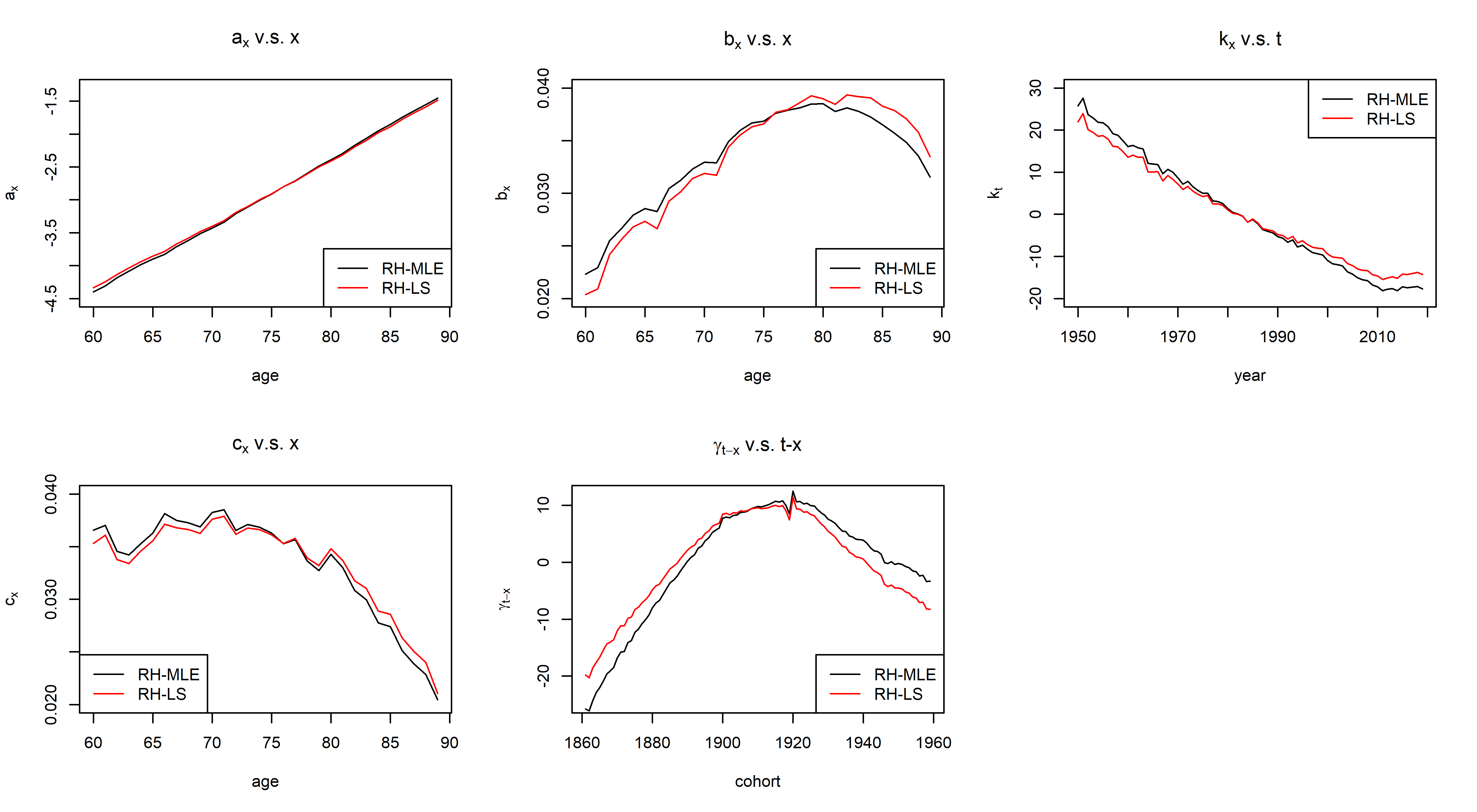
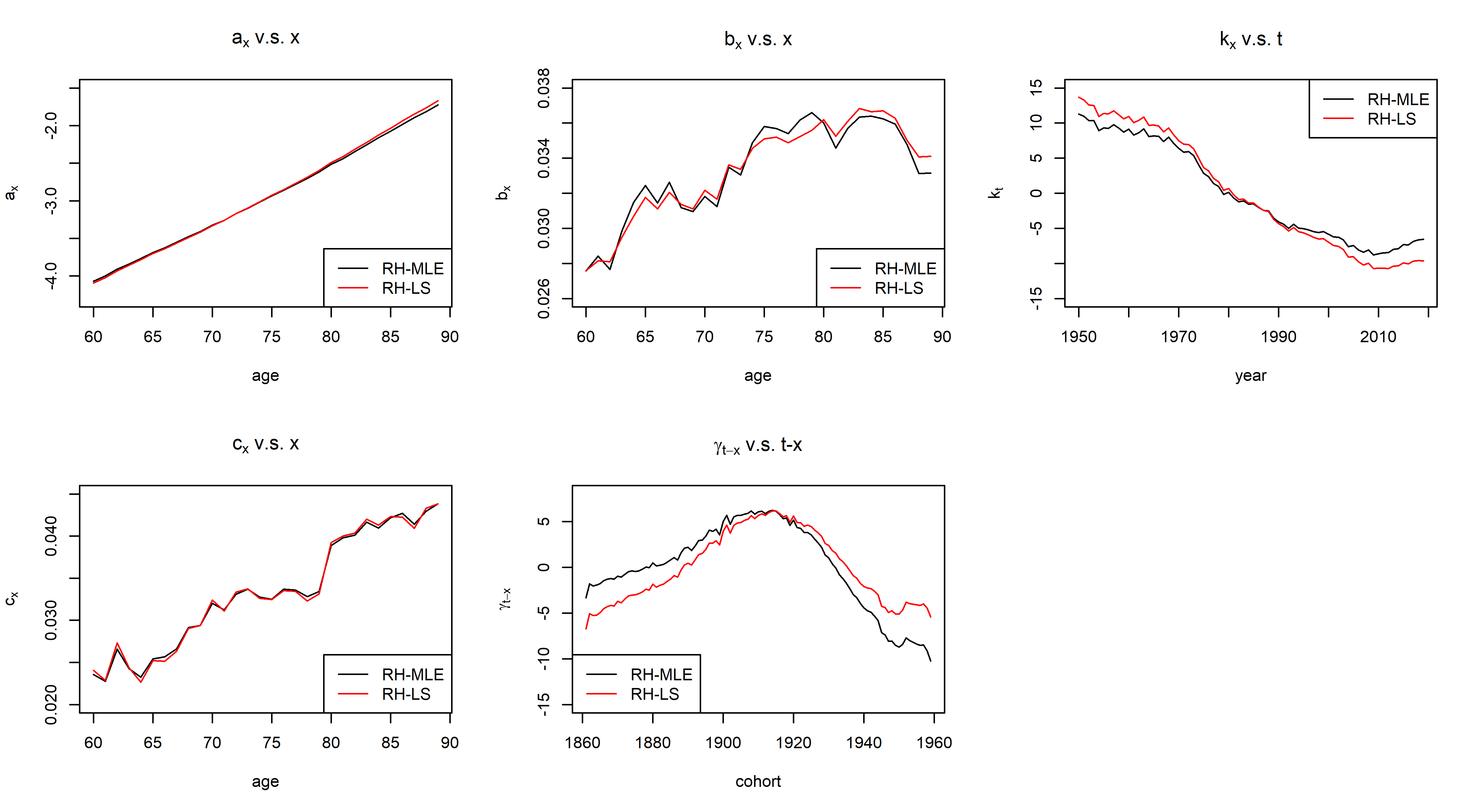
Figure 1: Parameter Estimates for RH-MLE and RH-LS for the E&W male dataset.

Figure 2: Parameter Estimates for RH-MLE and RH-LS for the USA male dataset.

The slight discrepancies in the parameter estimates between the two methods are further emphasized in Table 1, by the corresponding differences in the fitted $L^{2}$ errors and log-likelihoods. Since RH-LS is designed to minimize total $L^{2}$ error and RH-MLE maximizes the log-likelihood, which are essentially two different optimization problems, it is unsurprising that RH-LS yields a lower fitted $L^{2}$ error and a lower log-likelihood for the same dataset.

Data		RH-MLE	RH-LS	RH-MLE-Constr
E&W male	$L^{2}$ error	$0.578$	$\bm{0.565}$	$0.581$
	Log-likelihood	$\bm{-12843}$	$-12890$	$-12853$
	Computing time (s)	$336.68$	$38.72$	$\bm{20.39}$
USA male	$L^{2}$ error	$0.472$	$\bm{0.465}$	$0.473$
	Log-likelihood	$\bm{-17736}$	$-17828$	$-17744$
	Computing time (s)	$228.72$	$\bm{10.44}$	$25.95$

Table 1: Total $L^{2}$ error, fitted log-likelihood, and computing time for the Renshaw-Haberman model with different estimating methods. Datasets: E&W male and USA male.

Computing time (s)
Data	RH-MLE	RH-LS	RH-MLE-Constr
E&W female	$132.21$	$36.28$	$\bm{10.26}$
USA female	$30.23$	$\bm{26.18}$	$42.41$
Australia male	$53.10$	$\bm{5.76}$	$18.28$
Australia female	$59.12$	$\bm{10.81}$	$12.76$
Canada male	$118.51$	$\bm{16.17}$	$29.98$
Canada female	$59.02$	$\bm{11.71}$	$43.31$
Netherlands male	$101.22$	$\bm{13.58}$	$15.34$
Netherlands female	$39.25$	$24.52$	$\bm{5.62}$

Table 2: Computing time for the Renshaw-Haberman model with different estimating methods on the alternative datasets.

To demonstrate the robustness of our findings, we conducted similar analysis on several alternative datasets. These include female mortality data from England and Wales (E&W) and the USA, complementing our primary male datasets, along with data for both genders from Australia, Canada, and the Netherlands. The results, summarized in Table 2, consistently show that RH-LS significantly reduces computing time compared to RH-MLE, across all these datasets. This underscores the computational efficiency of the proposed least squares method, suggesting its potential as a compelling alternative to traditional MLE methods. Notably, the least squares algorithm achieves results comparable to traditional methods in both $L^{2}$ error and log-likelihood, but in considerably less time.

In Tables 1 and 2, we also note that RH-MLE-Constr generally improves computational speed relative to RH-MLE, competing closely with our RH-LS method in terms of efficiency. However, when comparing the goodness of fit between RH-LS and RH-MLE-Constr, careful interpretation is necessary. RH-MLE-Constr often results in a lower log-likelihood and higher $L^{2}$ error than RH-LS. This outcome is due to the fact that RH-MLE-Constr, despite incorporating an additional constraint, is still predominantly based on log-likelihood as its objective function. Consequently, it is not straightforward to conclusively determine whether RH-LS or RH-MLE-Constr offers better computational efficiency without significantly sacrificing goodness of fit. Moreover, as detailed in Section 3, RH-LS holds inherent advantages concerning model assumptions. Unlike RH-MLE-Constr, which assumes specific distributions (typically Poisson) for mortality data and imposes additional constraints on the estimated $\bm{\gamma}$ curve to enhance computation, RH-LS relies solely on the $L^{2}$ error as its objective function, without additional distributional assumptions.

6.2 Further Comparison between RH-LS and RH-MLE

The computational advantage of the least squares methods over the MLE methods could be explained by the sharpness of the objective function close to the optimal solution. Cairns et al. (2009) commented on the classical MLE method that “the likelihood function will be close to flat in certain dimensions”, which could result in the classical MLE methods being sensitive to the tolerance level $\delta$. As a result from the flatness of the objective function, the MLE methods could show different patterns for the estimated parameters and take a significantly longer time to fit the model, but with only minimal improvements in the objective function.

	Tolerance Level	RH-MLE	RH-LS
$L^{2}$ error	$10^{-6}$	$0.4734$	$0.4661$
	$10^{-7}$	$0.4727$	$0.4654$
	$10^{-8}$	$0.4720$	$0.4652$
Log-likelihood	$10^{-6}$	$-17749$	$-17828$
	$10^{-7}$	$-17745$	$-17827$
	$10^{-8}$	$-17737$	$-17827$
Time (sec)	$10^{-6}$	$12.28$	$3.96$
	$10^{-7}$	$20.67$	$4.92$
	$10^{-8}$	$283.87$	$11.28$

Table 3: $L^{2}$ error, fitted log-likelihood, and computing time (s) for RH-MLE and RH-LS with different tolerance levels for the USA male dataset.

To make the arguments clear, we fit RH-MLE and RH-LS to the USA male mortality data, with three different tolerance levels $10^{-6}$, $10^{-7}$ and $10^{-8}$. Figure 3 reveals disparate parameter patterns fitted by RH-MLE across tolerance levels, showing the fitted parameters prove sensitive to variations in the tolerance level. However, it can observed from Table 3 that these changes only result in marginal improvements in the objective function (log-likelihood), at the cost of substantially increased computational time.

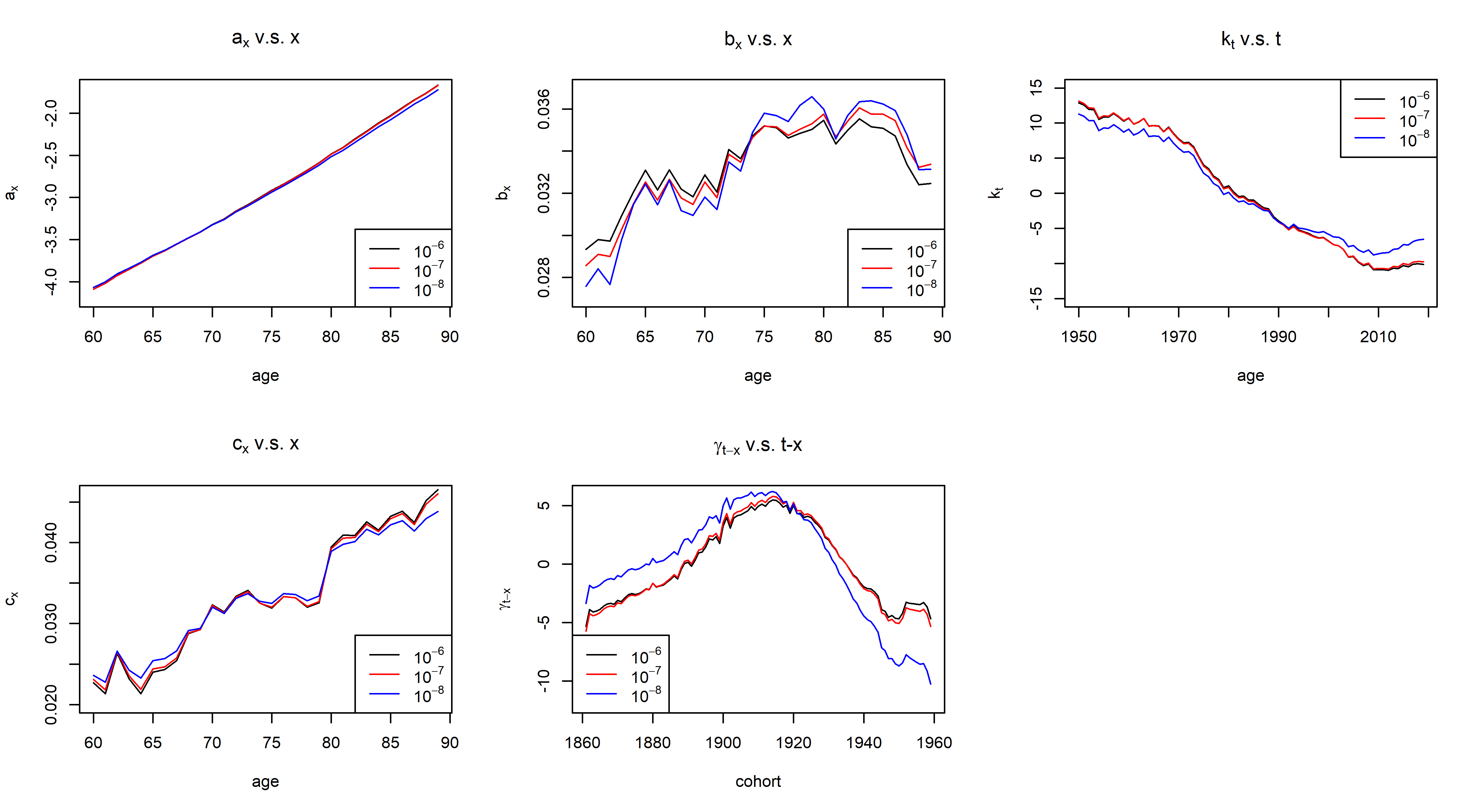
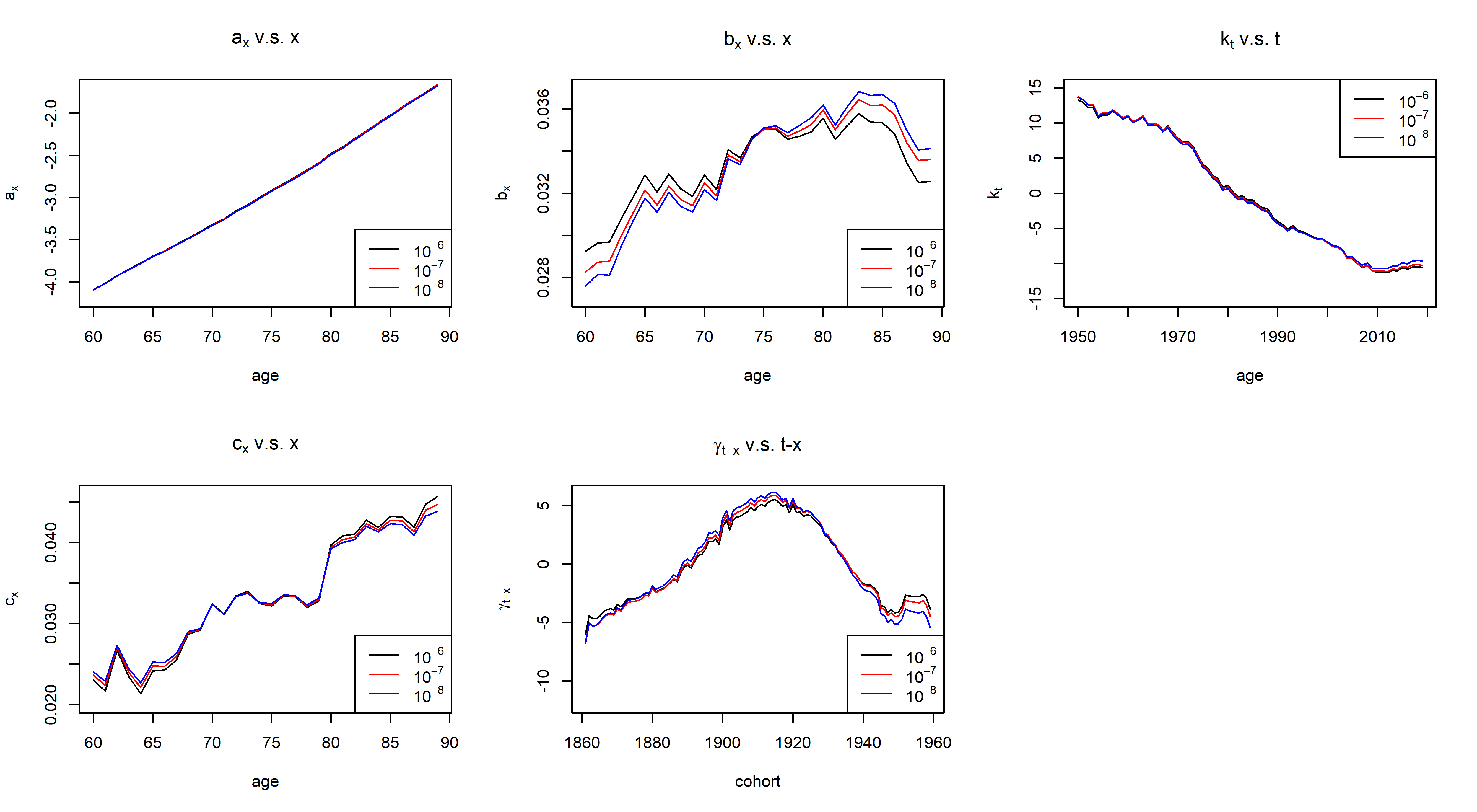
Figure 3: Parameter estimates of the RH-MLE method with different tolerance levels.

Figure 4: Parameter estimates of the RH-LS method with different tolerance levels.

Conversely, RH-LS shows greater robustness to changes in the tolerance level. This is evident from Figure 4, where the curves representing the estimated parameters are closely aligned across all tolerance levels. Additionally, the increase in computational time is moderate in comparison to RH-MLE. These outcomes suggest that the objective function for RH-LS, which is the $L^{2}$ error (total sum of square errors), is less flat near the optimal point compared to the log-likelihood function for RH-MLE. It supports our observations from Tables 1-2 that RH-LS is computationally more efficient than RH-MLE.

6.3 Comparing the Least Squares Method and the MLE method for the H1 Model

In Section 5, we explored the application of our least squares estimation method to the H1 model (3.4), a simpler variant of the Renshaw-Haberman model. Despite its reduced parameter count (as $c_{x}=1/p$ is fixed), the H1 model can still encounter computational challenges with the MLE approach. Following a similar experimental design as in Section 6.1 for the Renshaw-Haberman model, we examine four methods for fitting the H1 model:

• H1-MLE: Classical MLE-based method for the H1 model, under the Poisson GLM framework;

• H1-MLE-Constr: MLE-based method for the H1 model under the Poisson GLM framework, with the additional constraint $\sum_{s}(s-\bar{s})\gamma_{s}=0$;

• H1-LS: Proposed least squares method for the H1 model, described in Section 5.1;

• H1-LS-Constr: Proposed least squares method for the H1 model,, with the additional constraint $\sum_{s}(s-\bar{s})\gamma_{s}=0$, described in Section 5.2.

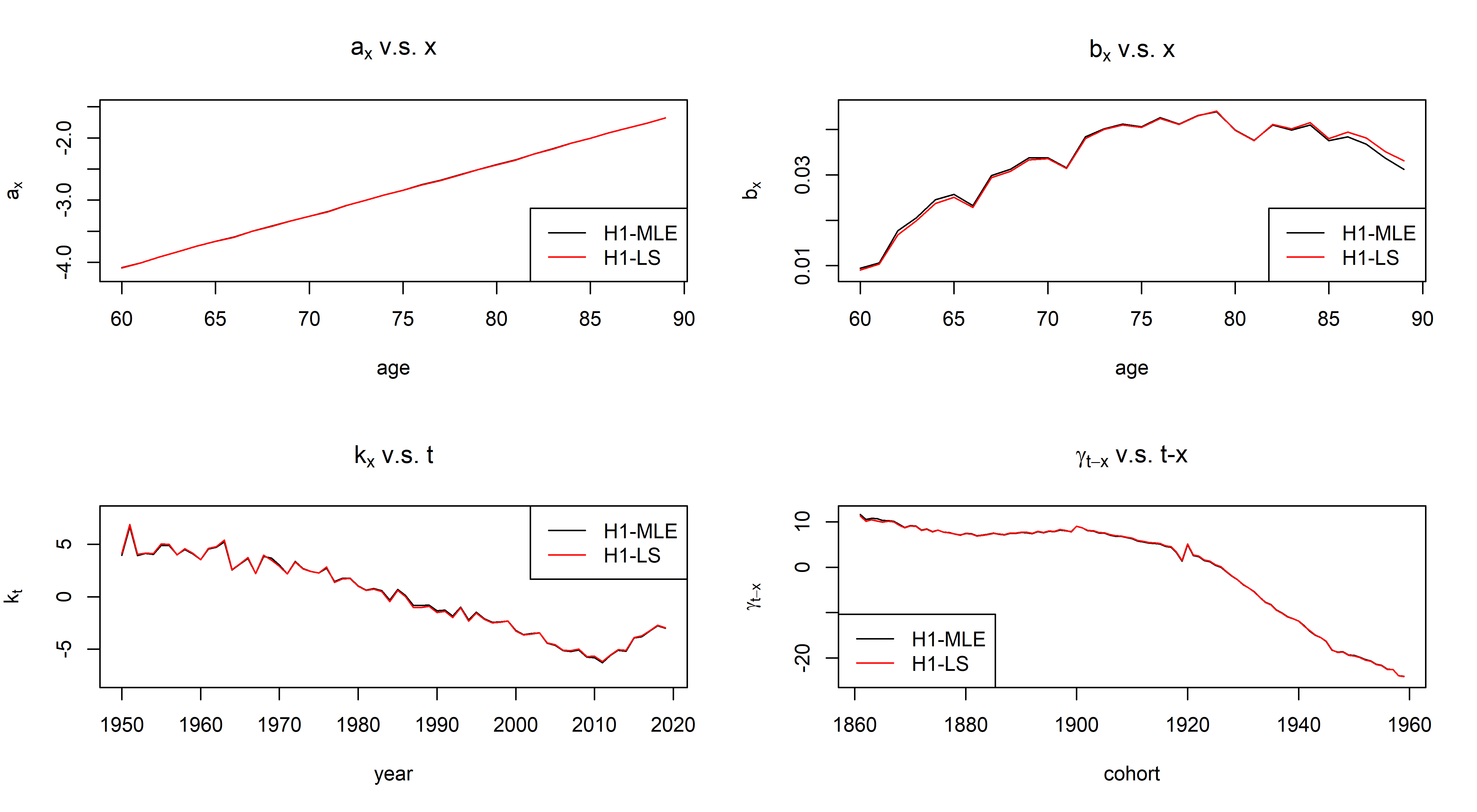
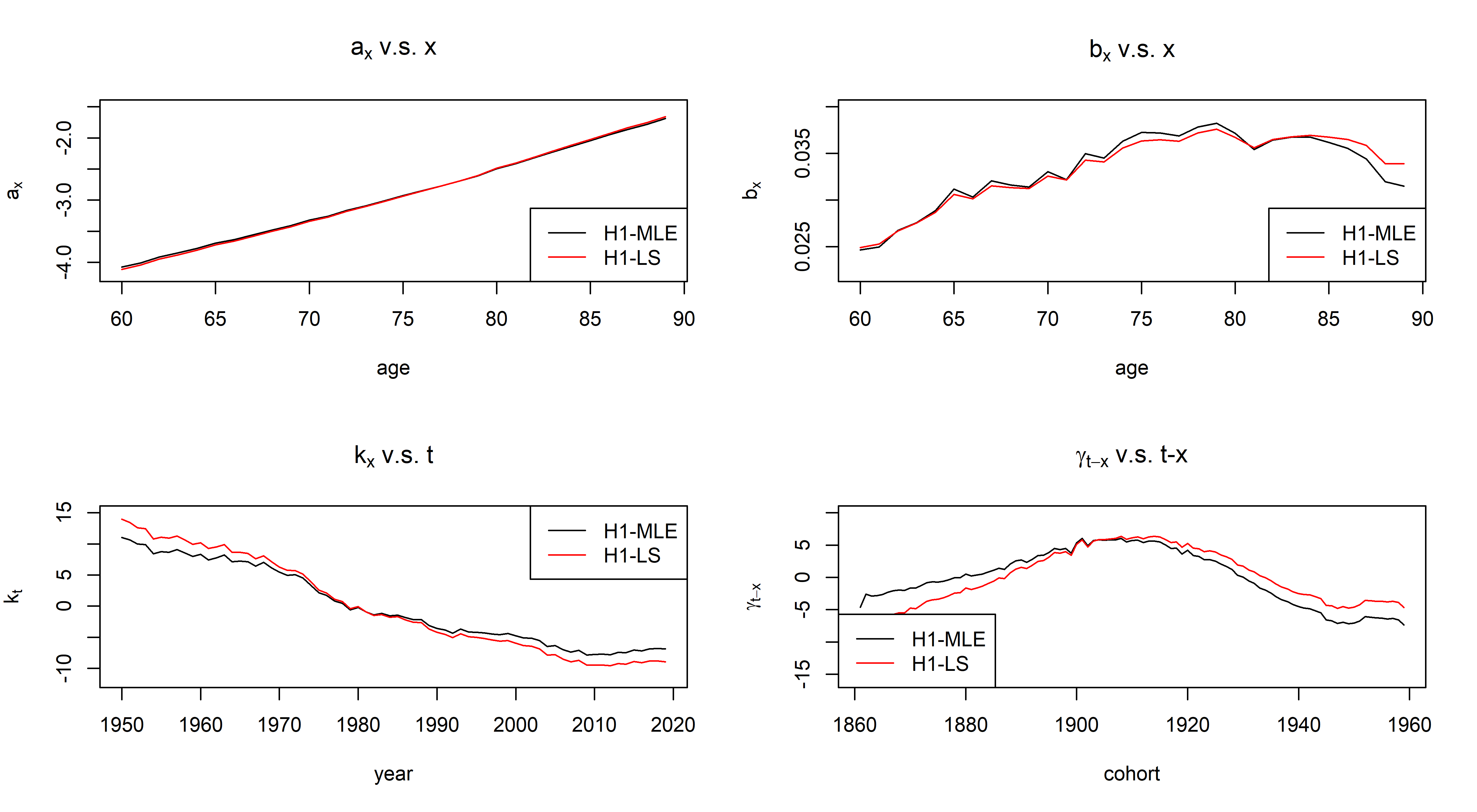
Figure 5: Parameter Estimates for H1-MLE and H1-LS for the E&W male dataset.

Figure 6: Parameter Estimates for H1-MLE and H1-LS for the USA male dataset.

Data		H1-MLE	H1-LS	H1-MLE-Constr	H1-LS-Constr
E&W male	$L^{2}$ error	$0.682$	$\bm{0.663}$	$0.721$	$0.697$
	Log-likelihood	$\bm{-13149}$	$-13208$	$-13247$	$-13321$
	Computing time (s)	$62.25$	$9.79$	$19.05$	$\bm{3.16}$
USA male	$L^{2}$ error	$0.557$	$\bm{0.545}$	$0.557$	$0.545$
	Log-likelihood	$\bm{-18692}$	$-18817$	$-18699$	$-18816$
	Computing time (s)	$138.88$	$2.56$	$18.30$	$\bm{2.12}$

Table 4: Total $L^{2}$ error, fitted log-likelihood, and computing time for the H1 model with different methods.

Computing time (s)
Data	H1-MLE	H1-LS	H1-MLE-Constr	H1-LS-Constr
E&W female	$58.23$	$1.12$	$7.58$	$\bm{0.97}$
USA female	$702.34$	$89.93$	$3.58$	$\bm{1.01}$
Australia male	$18.23$	$7.24$	$12.09$	$\bm{2.55}$
Australia female	$9.12$	$5.58$	$6.61$	$\bm{1.68}$
Canada male	$18.51$	$\bm{2.69}$	$15.23$	$3.42$
Canada female	$162.26$	$78.62$	$7.28$	$\bm{2.33}$
Netherlands male	$21.22$	$2.76$	$9.38$	$\bm{1.59}$
Netherlands female	$425.69$	$85.51$	$2.85$	$\bm{0.36}$

Table 5: Computing time for the H1 model with different estimating methods on the alternative datasets.

Table 4 presents similar findings for the H1 model, where H1-LS delivers satisfactory estimation results with significantly reduced computing time compared to H1-MLE. Compared to the full Renshaw-Haberman model, the H1 model tends to exhibit lower log-likelihoods and higher $L^{2}$ errors, reflecting a reduced goodness-of-fit. This outcome is inherently linked to the H1 model’s nature as a simplified version of the Renshaw-Haberman model. Owing to its simpler structure, the H1 model typically achieves faster fitting times. Furthermore, the disparity in parameter estimates between H1-MLE and H1-LS methods becomes less significant compared the Renshaw-Haberman model (RH-MLE and RH-LS), which is a possible consequence of the more restricted model structure of H1. For a comprehensive analysis, Table 5 includes results from similar analyses conducted on the alternative datasets mentioned in Section 6.1. These results consistently demonstrate the computational superiority of H1-LS over H1-MLE across various datasets.

Table 5 also indicates that for certain datasets, such as USA female, Canada female, and Netherlands female, fitting with RH-MLE and RH-LS is time-consuming, hinting at potential convergence issues possibly caused by the approximate identification problem (5.8). The introduction of an additional constraint in both H1-MLE-Constr and H1-LS-Constr could significantly enhances algorithm speed. While these methods are sufficiently rapid for individual implementations, H1-LS-Constr is still faster thn H1-MLE-Constr across all datasets, and the speed differences become more pronounced in scenarios requiring numerous repetitions. An example is bootstrapping for parameter uncertainty assessment, which involves resampling data and rerunning the estimation algorithm thousands of times. In such cases, the computational efficiency of H1-LS-Constr is particularly beneficial, underscoring the versatility and strength of our proposed least squares framework, especially when combined with existing methodologies to further improve algorithm speed.

6.4 Practical Considerations of Choosing Tolerance Levels for RH-LS

For most of the estimating methods, such as RH-MLE, they incorporate a single tolerance level $\delta$ that determines the convergence of the algorithm. On Contrary, RH-LS involves Algorithm 2, the iterative SVD algorithm, to update the values of $\bm{c}$ and $\bm{\gamma}$ in each iteration. Therefore, apart from the “global” tolerance level, defined as $\delta$ in (6.3) in this paper, RH-LS distinctly requires another “local” tolerance level, denoted as $\eta$. This tolerance level, that determines the convergence of Algorithm 2, is defined as the relative change in the $L^{2}$ error of each iteration when updating $\bm{c}$ and $\bm{\gamma})$ within the main iterative process:

$$L(\bm{c},\bm{\gamma})=\sum_{x,t}(\underbrace{(y_{x,t}-a_{x}-b_{x}k_{t})}_{\text{given}}-c_{x}\gamma_{t-x})^{2}.$$ (6.4)

It is worth noting that the variant H1-LS does not involve such local tolerance, because of the close-form formulas to update the cohort parameters $\bm{\gamma}$, as discussed in Section 5.1.

The choice of the local tolerance $\eta$ is somewhat arbitrary. For the global tolerance $\delta$, it is true that a lower $\delta$ will yield higher accuracy at the expense of a longer computing time, however, this trade-off does not apply to the local tolerance $\eta$ in our setting. When lowering $\eta$, it can provide a more accurate update for $(\bm{c},\bm{\gamma})$ at each main iterative step in the outer loop, Algorithm 1. Although this may require more computations and potentially slow down the inner loop, Algorithm 2, the improved accuracy from the inner loop could reduce the total number of iterations needed in outer loop for convergence. Therefore, the effect of changing $\eta$ on the overall convergence rate is not monotonic.

To examine this effect quantitatively, we fit RH-LS to the E&W dataset under different combinations of tolerance levels $(\delta,\eta)$, ranging from $10^{-5}$ to $10^{-8}$, and summarize the results in Table 3. First, we observe smaller $L^{2}$ errors associated with a longer computing when we decrease the global tolerance $\delta$. This is expected, as reducing $\delta$ allows the algorithm to produce more accurate estimates, but it takes longer to run. The non-monotonicity of the local tolerance $\eta$ can be demonstrated by the results of $\delta=10^{-8}$, which produce virtually the same $L^{2}$ errors, but $\eta=10^{-6}$ has the shortest runtime. This suggests that in practice, it is generally not advisable to set $\eta$ too low or too high, and we choose $\eta=10^{-6}$ in this study, including all the numerical results presented in Section 6.1.

	Tolerance	$\delta=10^{-5}$	$\delta=10^{-6}$	$\delta=10^{-7}$	$\delta=10^{-8}$
$L^{2}$ error	$\eta=10^{-5}$	$0.578$	$0.568$	$0.567$	$0.565$
	$\eta=10^{-6}$	$0.574$	$0.567$	$0.566$	$0.565$
	$\eta=10^{-7}$	$0.573$	$0.567$	$0.566$	$0.565$
	$\eta=10^{-8}$	$0.572$	$0.567$	$0.566$	$0.564$
Computing time (s)	$\eta=10^{-5}$	$1.62$	$2.76$	$4.31$	$40.87$
	$\eta=10^{-6}$	$3.34$	$4.49$	$5.70$	$37.21$
	$\eta=10^{-7}$	$7.17$	$9.51$	$10.81$	$38.23$
	$\eta=10^{-8}$	$15.14$	$20.13$	$22.95$	$66.55$

Table 6: Total $L^{2}$ error and computing time (s) for RH-LS with different combinations of tolerance levels.

7 Conclusion

In this paper, we have introduced a least squares method for estimating the parameters of the Renshaw-Haberman model. Our approach directly minimizes the total $L^{2}$ error, which measures the discrepancy between the observed and fitted log mortality rates. To accomplish this, we have employed an alternating minimization scheme that iteratively updates the model parameters. A key challenge we encountered was updating the age-cohort component $c_{x}\gamma_{t-x}$, which we addressed by formulating it as a PCA problem with missing values. This was effectively solved using an iterative SVD algorithm. Through numerical experiments using mortality data for multiple populations, we have demonstrated that our method significantly outperforms the traditional MLE-based method via iterative Newton-Raphson, in terms of computational efficiency, and produces satisfactory estimation results.

Additionally, we have adapted our method to the Renshaw-Haberman model variants, especially the H1 model. Here, the model’s simplicity allows for computational gains through single-step explicit updates for $\gamma_{t-x}$. We also showed that our least squares method can be harmoniously integrated with existing approaches to address computational challenges in the Renshaw-Haberman model. This includes incorporating the identification constraint by Hunt and Villegas (2015), for which we developed corresponding closed-form formulas.

The main objectives of this paper were two-fold. Firstly, we aimed to develop a fast estimation method for the Renshaw-Haberman model and its variants to address the issue of slow convergence commonly encountered with existing methods. Secondly, we aimed to fill the gap in the literature regarding least-squares-based estimation methods for the Renshaw-Haberman model, despite the SVD approach having been proposed earlier than the Poisson GLM method for the Lee-Carter model.

Future research building on this work could extend the proposed least squares method to a broader range of mortality models, notably the Cairns-Blake-Dowd (CBD) model incorporating cohort effects. The original CBD model, proposed by (Cairns et al., 2006), employed a least squares method for parameter estimation, benefiting from its simplicity in the absence of cohort effects. However, cohort-extended versions of the CBD model currently rely solely on MLE methods, highlighting a significant area for further research. In conjunction with this paper’s contributions, our next objective is to develop a comprehensive R package for stochastic mortality modelling based on the least squares approach. This package aims to encompass a wide class of mortality models, offering a valuable complement to the existing StMoMo package, which is primarily based on the MLE framework.

Appendix: Theoretical Properties of the Iterative SVD Algorithm

In this appendix, we provide more technical details about the iterative SVD algorithm described in Algorithm 2.

Recall that the objective optimization problem is to update the age-cohort parameters $(\bm{c},\bm{\gamma})$ by minimizing the target loss function:

$$L(\bm{c},\bm{\gamma})=\sum_{x,s\in\mathcal{O}}(z_{x,s}-c_{x}\gamma_{s})^{2},$$ (A.1)

where $s=t-x$ is the cohort and $\mathcal{O}$ is the set of index of observed values. For sake of the notational clarity, we use $\hat{z}_{x,s}(\bm{\theta}):=c_{x}\gamma_{s}$ to denote the estimator of the observation $z_{x,s}$, as a function of the model parameters $\bm{\theta}=(\bm{c},\bm{\gamma})$. Thus, we can rewrite the optimization problem as finding $\bm{\theta}$ to minimize the $L^{2}$ loss function of the observed data:

$$L_{obs}(\bm{\theta})=\sum_{x,s\in\mathcal{O}}(z_{x,s}-\hat{z}_{x,s}(\bm{\theta}))^{2}.$$ (A.2)

The iterative SVD algorithm, rather than directly solving (A.2), iteratively performs imputation and SVD on the complete data matrix $\bm{Z}_{c}$. Let us write the $L^{2}$ loss function of the complete data and missing data as:

$$L_{tot}(\bm{\theta},\tilde{\bm{z}})=L_{obs}(\bm{\theta})+L_{mis}(\bm{\theta},\tilde{\bm{z}})$$ (A.3)

$$L_{mis}(\bm{\theta},\tilde{\bm{z}})=\sum_{x,s\notin\mathcal{O}}(\tilde{z}_{x,s}-\hat{z}_{x,s}(\bm{\theta}))^{2},$$ (A.4)

where $\tilde{z}_{x,s}$ is the imputed missing value. The iterative SVD algorithm minimizes the total $L^{2}$ error (A.3) as a function $L_{tot}(\bm{\theta},\tilde{\bm{z}})$ with respect to both the model parameter $\bm{\theta}$ and the set of imputed values $\tilde{\bm{z}}=\{\tilde{z}_{x,s}|x,s\notin\mathcal{O}\}$.

Convergence of the Iterative SVD Algorithm

We first show that the iterative SVD algorithm always converges by showing that the algorithm can be represented as an alternating minimization procedure:

1. For a fixed $\tilde{\bm{z}}$, let $\bm{\theta}^{\ast}$ be the minimizer of $L_{tot}(\bm{\theta},\tilde{\bm{z}})$ with respect to $\bm{\theta}$:

   $$\bm{\theta}^{\ast} =\arg\min_{\bm{\theta}}L_{tot}(\bm{\theta},\tilde{\bm{z}})$$

   $$=\arg\min_{\bm{\theta}}\left[\sum_{x,s\in\mathcal{O}}(z_{x,s}-\hat{z}_{x,s}(\bm{\theta}))^{2}+\sum_{x,s\notin\mathcal{O}}(\tilde{z}_{x,s}-\hat{z}_{x,s}(\bm{\theta}))^{2}\right]$$

   $$=\arg\min_{\bm{\theta}}\left[\sum_{x,s}(z^{\prime}_{x,s}-\hat{z}_{x,s}(\bm{\theta}))^{2}\right],$$ (A.5)

   where $z^{\prime}_{x,s}$ denotes the data with imputed missing values, which equals $z_{x,s}$ for $x,s\in\mathcal{O}$ and equals $\tilde{z}_{x,s}$ for $x,s\notin\mathcal{O}$. Since $\hat{z}_{x,s}(\bm{\theta}):=c_{x}\gamma_{s}$, the minimizer $\bm{\theta}^{\ast}$ can be found by performing PCA to the approximate complete matrix $\bm{Z}_{c}$, as described in Step 2 of Algorithm 2.

2. For a fixed $\bm{\theta}$, let $\tilde{\bm{z}}^{\ast}$ be the minimizer of $L_{tot}(\bm{\theta},\tilde{\bm{z}})$ with respect to $\tilde{\bm{z}}$:

   $$\tilde{\bm{z}}^{\ast} =\arg\min_{\tilde{\bm{z}}}L_{tot}(\bm{\theta},\tilde{\bm{z}})$$

   $$=\arg\min_{\tilde{\bm{z}}}\left[L_{mis}(\bm{\theta},\tilde{\bm{z}})+\text{const.}\right]$$

   $$=\arg\min_{\tilde{\bm{z}}}\left[\sum_{x,s\notin\mathcal{O}}(\tilde{z}_{x,s}-\hat{z}_{x,s}(\bm{\theta}))^{2}+\text{const.}\right].$$ (A.6)

   It is straightforward to see that the minima is achieved when $\tilde{z}_{x,s}=\hat{z}_{x,s}(\bm{\theta})$ and so $\tilde{\bm{z}}^{\ast}=\{\tilde{z}_{x,s}(\bm{\theta})|x,s\notin\mathcal{O}\}$. This solution is exactly imputing the missing values by the PCA reconstruction $\hat{z}_{x,s}(\bm{\theta})$ with parameters $\bm{\theta}$, as described in Step 3 of Algorithm 2.

The Iterative SVD Algorithm Minimizes the Target Loss Function

We next show that the iterative SVD algorithm minimizes the target loss function (A.2). More precisely, the minimizer $\bm{\theta}^{\ast}$ obtained by iteratively minimizing the total $L^{2}$ error $L_{tot}(\bm{\theta},\tilde{\bm{z}})$ is equivalent to the one obtained by directly minimizing the $L^{2}$ error $L_{obs}(\bm{\theta})$ of the observed data.

Following (A.6),

$$\tilde{\bm{z}}^{\ast}=\arg\min_{\tilde{\bm{z}}}L_{tot}(\bm{\theta},\tilde{\bm{z}})=\arg\min_{\tilde{\bm{z}}}\left[\sum_{x,s\notin\mathcal{O}}(\tilde{z}_{x,s}-\hat{z}_{x,s}(\bm{\theta}))^{2}\right],$$ (A.7)

which immediately implies that

$$\frac{\partial L_{tot}}{\partial\tilde{\bm{z}}}\Bigg{|}_{\tilde{\bm{z}}=\tilde{\bm{z}}^{\ast}}=0$$ (A.8)

and

$$L_{mis}(\bm{\theta},\tilde{\bm{z}}^{\ast})=\sum_{x,s\notin\mathcal{O}}(\hat{z}_{x,s}(\bm{\theta})-\hat{z}_{x,s}(\bm{\theta}))^{2}=0,$$ (A.9)

Therefore, we can obtain

$$L_{tot}(\bm{\theta},\tilde{\bm{z}}^{\ast})=L_{obs}(\bm{\theta})+L_{mis}(\bm{\theta},\tilde{\bm{z}}^{\ast})=L_{obs}(\bm{\theta}).$$ (A.10)

and consequentially,

$$\frac{dL_{obs}}{d\bm{\theta}}=\frac{dL_{tot}}{d\bm{\theta}}\Bigg{|}_{\tilde{\bm{z}}=\tilde{\bm{z}}^{\ast}}=\frac{\partial L_{tot}}{\partial\bm{\theta}}\Bigg{|}_{\tilde{\bm{z}}=\tilde{\bm{z}}^{\ast}}+\underbrace{\frac{\partial L_{tot}}{\partial\tilde{\bm{z}}}\Bigg{|}_{\tilde{\bm{z}}=\tilde{\bm{z}}^{\ast}}}_{=0\text{ from }\eqref{partial=0}}\cdot\frac{\partial\tilde{\bm{z}}}{\partial\bm{\theta}}=\frac{\partial L_{tot}}{\partial\bm{\theta}}\Bigg{|}_{\tilde{\bm{z}}=\tilde{\bm{z}}^{\ast}}$$ (A.11)

which suggests that the minimizer $\bm{\theta}^{\ast}$ of $L_{tot}(\bm{\theta},\bm{z}_{imp})$ coincides with the minimizer of $L_{obs}(\bm{\theta})$, and thus shows that the iterative SVD algorithm indeed implicitly solves our objective optimization problem (4.11).

References

- Brouhns et al. (2002) Brouhns, N., Denuit, M., & Vermunt, J. K. (2002). A Poisson log-bilinear regression approach to the construction of projected lifetables. Insurance: Mathematics and economics, 31(3), 373-393.
- Cairns et al. (2006) Cairns, A. J., Blake, D., & Dowd, K. (2006). A two‐factor model for stochastic mortality with parameter uncertainty: theory and calibration. Journal of Risk and Insurance, 73(4), 687-718.
- Cairns et al. (2011) Cairns, A. J., Blake, D., Dowd, K., Coughlan, G. D., Epstein, D., & Khalaf-Allah, M. (2011). Mortality density forecasts: An analysis of six stochastic mortality models. Insurance: Mathematics and Economics, 48(3), 355-367.
- Cairns et al. (2009) Cairns, A. J., Blake, D., Dowd, K., Coughlan, G. D., Epstein, D., Ong, A., & Balevich, I. (2009). A quantitative comparison of stochastic mortality models using data from England and Wales and the United States. North American Actuarial Journal, 13(1), 1-35.
- Currie (2016) Currie, I. D. (2016). On fitting generalized linear and non-linear models of mortality. Scandinavian Actuarial Journal, 2016(4), 356-383.
- Fung (2018) Fung, M. C., Peters, G. W., & Shevchenko, P. V. (2018). Cohort effects in mortality modelling: A Bayesian state-space approach. Annals of Actuarial Science, 13(1), 109-144.
- Goodman (1979) Goodman, L. A. (1979). Simple models for the analysis of association in cross-classifications having ordered categories. Journal of the American Statistical Association, 74(367), 537-552.
- Haberman and Renshaw (2009) Haberman, S., & Renshaw, A. (2009). On age-period-cohort parametric mortality rate projections. Insurance: Mathematics and Economics, 45(2), 255-270.
- Haberman and Renshaw (2011) Haberman, S., & Renshaw, A. (2011). A comparative study of parametric mortality projection models. Insurance: Mathematics and Economics, 48(1), 35-55.
- Hobcraft et al. (1982) Hobcraft, J., Menken, J., & Preston, S. (1982). Age, period, and cohort effects in demography: a review. Population Index, 48(1), 35-55.
- Human Mortality Database (HMD) Human Mortality Database. (2023) Max Planck Institute for Demographic Research, University of California, Berkeley, and French Institute for Demographic Studies. Available at www.mortality.org.
- Hunt and Blake (2021) Hunt, A., & Blake, D. (2021). On the structure and classification of mortality models. North American Actuarial Journal, 25(sup1), S215-S234.
- Hunt and Villegas (2015) Hunt, A., & Villegas, A. M. (2015). Robustness and convergence in the Lee–Carter model with cohort effects. Insurance: Mathematics and Economics, 64, 186-202.
- Ilin and Raiko (2010) Ilin, A., & Raiko, T. (2010). Practical approaches to principal component analysis in the presence of missing values. The Journal of Machine Learning Research, 11, 1957-2000.
- Koissi et al. (2006) Koissi, M. C., Shapiro, A. F., & Högnäs, G. (2006). Evaluating and extending the Lee–Carter model for mortality forecasting: Bootstrap confidence interval. Insurance: Mathematics and Economics, 38(1), 1-20.
- Lee and Carter (1992) Lee, R. D., & Carter, L. R. (1992). Modeling and forecasting US mortality. Journal of the American statistical association, 87(419), 659-671.
- Leng and Peng (2016) Leng, X., & Peng, L. (2016). Inference pitfalls in Lee–Carter model for forecasting mortality. Insurance: Mathematics and Economics, 70, 58-65.
- Liu et al. (2019) Liu, Q., Ling, C., & Peng, L. (2019). Statistical inference for Lee-Carter mortality model and corresponding forecasts. North American Actuarial Journal, 23(3), 335-363.
- Mazumder et al. (2010) Mazumder, R., Hastie, T., & Tibshirani, R. (2010). Spectral regularization algorithms for learning large incomplete matrices. The Journal of Machine Learning Research, 11, 2287-2322.
- Renshaw and Haberman (2003) Renshaw, A. E., & Haberman, S. (2003). Lee–Carter mortality forecasting with age-specific enhancement. Insurance: Mathematics and Economics, 42(3), 575-594.
- Renshaw and Haberman (2006) Renshaw, A. E., & Haberman, S. (2006). A cohort-based extension to the Lee–Carter model for mortality reduction factors. Insurance: Mathematics and economics, 38(3), 556-570.
- Villegas and Haberman (2014) Villegas, A. M., & Haberman, S. (2014). On the modeling and forecasting of socioeconomic mortality differentials: An application to deprivation and mortality in England. North American Actuarial Journal, 18(1), 168-193.
- Villegas et al. (2015) Villegas, A., Kaishev, V. K., & Millossovich, P. StMoMo: An R package for stochastic mortality modelling. 7th Australasian Actuarial Education and Research Symposium, 2015.
- Willets (2004) Willets, R. C. (2004). The cohort effect: insights and explanations. British Actuarial Journal, 10(4), 833-877.
- Wilmoth (1990) Wilmoth, J. R. (1990). Variation in vital rates by age, period, and cohort. Sociological methodology, 20, 295-335.