Study of MMSE-Based Resource Allocation for Clustered Cell-Free Massive MIMO Networks

Abstract

In this paper, a downlink cell-free massive multiple-input multiple-output (CF massive MIMO) system and a network clustering is considered. Closed form sum-rate expressions are derived for CF and the clustered CF (CLCF) networks where linear precoders included zero forcing (ZF) and minimum mean square error (MMSE) are implemented. An MMSE-based resource allocation technique with multiuser scheduling based on an enhanced greedy technique and power allocation based on the gradient descent (GD) method is proposed in the CLCF network to improve the system performance. Numerical results show that the proposed technique is superior to the existing approaches and the computational cost and the signaling load are essentially reduced in the CLCF network.

I Introduction

Cell-free (CF) massive multiple-input multiple-output (MIMO) networks were initially proposed in [1, 2] where a large number of access points (APs) jointly serve all user equipments (UEs) using the same time frequency resources through a wide area. Thereby, a higher coverage rate and throughput could be provided compared to cellular networks. Regarding the huge burden imposed on the processing unit in CF networks, network clustering including user-centric and network-centric approaches are suggested in literature to make it practical in terms of signaling and computational complexity [3, 4, 5, 6, 7].

The downlink of MIMO networks [8, 9] require transmit processing techniques such as precoding [10, 11, 12, 13, 14, 15, 16, 17, 18, 19, 20, 21, 22, 23, 24, 25] and resource allocation [26, 27, 28, 29, 21, 30]. In particular, one of the most important concepts in CF networks in practice is resource allocation including multiuser scheduling and power allocation to improve network performance. Multiuser scheduling is fundamental in multiuser interference reduction [31] and power allocation is crucial to gain the desirable performance. These challenges are addressed in several works. In [32], downlink resource allocation in CF massive MIMO networks is studied through the maximization of the minimum achievable rate among the UEs. The work of [33] has studied a network slicing based CF massive MIMO architecture to support many UEs through resource slicing in a virtualized wireless CF massive MIMO network. A weighted sum-rate (WSR) problem was solved in [34] using fractional programming and employing compressive sensing for multiuser scheduling and power allocation in clustered CF (CLCF) massive MIMO networks.

In this paper, we investigate the downlink of CF and CLCF massive MIMO networks and investigate resource allocation techniques for sum-rate maximization. In particular, we derive closed form expressions for sum-rates of CF and CLCF massive MIMO networks and develop a sequential multiuser scheduling and power allocation (SMSPA) scheme. For the SMSPA scheme, we develop an improved greedy subset selection (IGSS) technique based on the algorithm proposed in [35] for user scheduling and devise a gradient descent (GD) power allocation algorithm for mean square error (MSE) minimization which is equivalent to sum-rate maximization as will be described later. Simulation results show the superiority of the proposed SMSPA scheme and resource allocation techniques as compared to existing methods.

Notation: Throughout the paper, $\left\|.\right\|_{F}$ denotes the Frobenius norm, $\textbf{I}_{N}\in\mathbb{C}^{N\times N}$ denotes the identity matrix, the complex normal distribution is represented by $\mathcal{CN}\left(.,.\right)$, superscripts ^T, ^∗, and ^H denote transpose, complex conjugate and hermitian operations respectively, $\mathcal{A}\cup\mathcal{B}$ is union of sets $\mathcal{A}$ and $\mathcal{B}$, $\mathcal{A}\setminus\mathcal{B}$ shows exclusion of set $\mathcal{B}$ from set $\mathcal{A}$, and ${Tr}\left(.\right)$ shows the Trace operator.

II System Model

We consider a CF network including $M$ randomly distributed single antenna APs and $K$ uniformly distributed single antenna UEs. The CLCF network is formed by dividing the CF network into $C$ non-overlapping areas where the cluster $c$ includes $M_{c}$ randomly distributed single antenna APs and $K_{c}$ uniformly distributed single antenna UEs. We assume that the number of UEs is much larger than the number of APs in both networks so that $K>>M$.

II-A CF and CLCF Networks

In the CF network including $M$ APs and and $K$ UEs, the channel between AP $m$ and UE $k$ is shown by the coefficient $g_{mk}=\sqrt{\beta_{mk}}h_{mk}$ [2], where $\beta_{mk}$ are the large-scale fading coefficients due to the path loss and shadowing and $h_{mk}\sim\mathcal{CN}\left(0,1\right)$ denote the independent and identically distributed (i.i.d.) random variables (RVs) modelling small-scale fading that remain constant during a coherence interval and which are assumed to be independent over different coherence intervals. Further, we assume the following model of the large scale coefficients $\beta_{mk}=\textup{PL}_{mk}\times 10^{\frac{\sigma_{sh}z_{mk}}{10}}$ where $\textup{PL}_{mk}$ is the path loss and $10^{\frac{\sigma_{sh}z_{mk}}{10}}$ refers to shadow fading where $\sigma_{sh}=8\textup{dB}$, $z_{mk}\sim\mathcal{N}\left(0,1\right)$. Considering $d_{mk}$ is the distance between the AP $m$ and UE $k$, the path loss is modeled using the results from [36] as

$$\textup{PL}_{mk}=\left\{\begin{matrix}-\textup{D}-35\log_{10}\left(d_{mk}\right),\textup{if }d_{mk}>d_{1}&\\ -\textup{D}-10\log_{10}\left(d_{1}^{1.5}d_{mk}^{2}\right),\textup{if }d_{0}<d_{mk}\leq d_{1}&\\ -\textup{D}-10\log_{10}\left(d_{1}^{1.5}d_{0}^{2}\right),\textup{if }d_{mk}\leq d_{0}&\end{matrix}\right.,$$ (1)

where

$$\begin{multlined}\textup{D}=46.3+33.9\log_{10}\left(f\right)-13.82\log_{10}\left(h_{AP}\right)\\ -\left[1.11\log_{10}\left(f\right)-0.7\right]h_{u}+1.56\log_{10}\left(f\right)-0.8\end{multlined}\textup{D}=46.3+33.9\log_{10}\left(f\right)-13.82\log_{10}\left(h_{AP}\right)\\ -\left[1.11\log_{10}\left(f\right)-0.7\right]h_{u}+1.56\log_{10}\left(f\right)-0.8$$ (2)

$f=1900$MHz is the carrier frequency, $h_{AP}=$15m and $h_{u}=$1.5m are the AP and UE antenna heights, respectively, $d_{0}=$10m and $d_{1}=$50m. When $d_{mk}\leq d_{1},$ there is no shadowing. The downlink signal received at $n$ scheduled UEs is given by

$$\mathbf{y}=\sqrt{\rho_{f}}\mathbf{G}^{T}\mathbf{P}\mathbf{x}+\mathbf{w}$$ (3)

where $\rho_{f}$ is the maximum transmitted power of each antenna, $\mathbf{G}=\hat{\textbf{G}}+\tilde{\textbf{G}}\in\mathbb{C}^{M\times n}$ is the channel matrix with the channel estimate $\hat{\textbf{G}}$ and the estimation error $\tilde{\textbf{G}}$ which models the CSI imperfection, $\left[\mathbf{G}\right]_{m,k}=g_{mk}$, $\mathbf{P}\in\mathbb{C}^{M\times n}$ is the linear precoder matrix, $\mathbf{x}=\left[x_{1},\cdots,x_{n}\right]^{T}$ is the zero mean symbol vector, $\mathbf{x}\sim\mathcal{CN}\left(\mathbf{0},\mathbf{I}_{n}\right)$, and $\mathbf{w}=\left[w_{1},\cdots,w_{n}\right]^{T}$ is the additive noise vector, $\textbf{w}\sim\mathcal{CN}\left(0,\sigma_{w}^{2}\textbf{I}_{n}\right)$. We consider elements of $\mathbf{x}$ to be mutually independent, and independent of all noise and channel coefficients. Thus, we can obtain the sum-rate of the CF system as follows

$$SR_{cf}=\log_{2}\left(\det\left[\textbf{R}_{cf}+\textbf{I}_{n}\right]\right)$$ (4)

where the covariance matrix $\textbf{R}_{cf}$ is given by

$$\textbf{R}_{cf}=\rho_{f}\hat{\textbf{G}}^{T}\textbf{P}\textbf{P}^{H}\hat{\textbf{G}}^{\ast}\left(\rho_{f}\tilde{\textbf{G}}^{T}\textbf{P}\textbf{P}^{H}\tilde{\textbf{G}}^{\ast}+\sigma_{w}^{2}\textbf{I}_{n}\right)^{-1}$$ (5)

When clustering is considered, the downlink received signal at $n_{c}$ scheduled UEs of the cluster $c$ is given by

$$\textbf{y}_{c}=\sqrt{\rho_{f}}{\textbf{G}}_{cc}^{T}\textbf{P}_{c}\textbf{x}_{c}+\sum_{i=1,i\neq c}^{C}\sqrt{\rho_{f}}{\textbf{G}}_{ic}^{T}\textbf{P}_{i}\textbf{x}_{i}+\textbf{w}_{c}$$ (6)

where $\textbf{G}_{ic}=\hat{\textbf{G}}_{ic}+\tilde{\textbf{G}}_{ic}\in\mathbb{C}^{M_{i}\times n_{c}}$ is the channel from APs of the cluster $i$ to the UEs of the cluster $c$, $\textbf{P}_{i}\in\mathbb{C}^{M_{i}\times n_{c}}$ is the linear precoding matrix, and $\textbf{x}_{i}=\left[x_{i1},\cdots,x_{in_{c}}\right]^{T}$ is the symbol vector of the cluster $i$, $\textbf{x}_{i}\sim\mathcal{CN}\left(\mathbf{0},\mathbf{I}_{n_{c}}\right)$, $i\in\left\{1,2,\cdots,C\right\}$, and $\textbf{w}_{c}=[w_{c_{1}},\cdots,w_{c_{n_{c}}}]^{T}$ is the additive noise vector, $\textbf{w}_{c}\sim\mathcal{CN}\left(0,\sigma_{w}^{2}\textbf{I}_{n_{c}}\right)$. Accordingly, the sum-rate expression for the cluster $c$ is obtained as

$$SR_{c}=\log_{2}\left(\det\left[\left(\rho_{f}\hat{\textbf{G}}_{cc}^{T}\textbf{P}_{c}\textbf{P}_{c}^{H}\hat{\textbf{G}}_{cc}^{*}\right)\textbf{R}_{c}^{-1}+\textbf{I}_{n_{c}}\right]\right)$$ (7)

and the covariance matrix $\textbf{R}_{c}$ is described by

$$\begin{split}\textbf{R}_{c}&=\rho_{f}\tilde{\textbf{G}}_{cc}^{T}\textbf{P}_{c}\textbf{P}_{c}^{H}\tilde{\textbf{G}}_{cc}^{*}+\sum_{i=1,i\neq c}^{C}\rho_{f}\hat{\textbf{G}}_{ic}^{T}\textbf{P}_{i}\textbf{P}_{i}^{H}\hat{\textbf{G}}_{ic}^{*}+\\ &\sum_{i=1,i\neq c}^{C}\rho_{f}\tilde{\textbf{G}}_{ic}^{T}\textbf{P}_{i}\textbf{P}_{i}^{H}\tilde{\textbf{G}}_{ic}^{*}+\sigma_{w}^{2}\textbf{I}_{n_{c}}\end{split}$$ (8)

where $\textbf{x}_{c}$ and $\textbf{w}_{c}$ are assumed to be statistically independent. Thus, the total network sum-rate is achieved by summation of Equation (7) over all clusters. At the receiver of the UEs several detection techniques [37, 38, 39, 40, 41, 42, 43] can be used.

III Proposed Resource Allocation Technique

For resource allocation in the CLCF network, in the proposed scheme, we first accomplish the multiuser scheduling according to the method implemented in [44], which determines various UE sets based on an enhanced greedy technique presented in [35] and considers equal power loading in the assignment of the sets and finally selects the best set according to the sum-rate criterion. Thereafter, a power allocation algorithm is proposed based on the gradient descent algorithm for MSE minimization. The proposed power allocation method significantly improves the sum-rate performance because MSE minimization is equivalent to the maximization of the Signal to interference plus noise ratio (SINR) which in turn is equivalent to the sum-rate maximization when Gaussian signaling is used [45]. Note that the proposed technique could be extended to be used in CF networks without clustering as well.

III-A User Scheduling Algorithm

Since the number of UEs is much larger than the number of APs, $K_{c}>>M_{c}$, we select the first set of UEs by adapting the implemented greedy method in [46] so that we can schedule a set of UEs with a pre-determined length. We consider an MMSE precoder unlike the ZF precoder used in [46] to improve the performance and the search algorithm. Considering $n_{c}$ as length of the selected set $\mathcal{S}_{n_{c}}$ and consequently the channel matrix $\textbf{G}_{cc}\left(\mathcal{S}_{n_{c}}\right)\in\mathbb{C}^{M_{c}\times{n_{c}}}$, the algorithm is the solution to the following problem

$${\max_{\mathcal{S}_{n_{c}}}~{}SR_{MMSE}({\mathcal{S}}_{n_{c}}})$$ (9)

$$\text{subject to}||\textbf{P}_{c}(\mathcal{S}_{n_{c}})||_{F}^{2}\leq P.$$

where $SR_{MMSE}({\mathcal{S}}_{n_{c}})$ is the sum-rate when MMSE precoder is used, $P$ is the upper limit of the signal covariance matrix ${Tr}[\textbf{C}_{\textbf{x}}]\leq P$ and $\textbf{P}_{c}(\mathcal{S}_{n_{c}})\in\mathbb{C}^{M_{c}\times{n_{c}}}$ is the precoding matrix. In the case of power allocation, the precoding matrix is defined as $\textbf{P}_{c}(\mathcal{S}_{n_{c}})=\textbf{W}_{c}\textbf{D}_{c}$ where $\textbf{W}_{c}\in\mathbb{C}^{M_{c}\times{n_{c}}}$ is the normalized MMSE weight matrix and $\textbf{D}_{c}\in\mathbb{C}^{{n_{c}}\times{n_{c}}}$ is the power allocation matrix considered as

$$\textbf{D}_{c}=\begin{bmatrix}\sqrt{p_{1}}&0&\cdots&0\\ 0&\sqrt{p_{2}}&\cdots&0\\ \vdots&\vdots&\cdots&\vdots\\ 0&0&\cdots&\sqrt{p_{{n_{c}}}}\end{bmatrix}=\textup{diag}\left(\textbf{d}_{c}\right)\\ ,\textbf{d}_{c}=\left[\sqrt{p_{1}}\ \sqrt{p_{2}}\ \cdots\ \sqrt{p_{{n_{c}}}}\right]^{T}.$$ (10)

In order to evaluate more sets of UEs so that we can approach the optimal set chosen by exhaustive search, we remove one UE from the set $\mathcal{S}_{{n_{c}}\left(1\right)}$ as the UE with the lowest channel power among the selected set and substitute it with another UE with the highest channel power from the remaining UEs other than $\mathcal{S}_{{n_{c}}\left(1\right)}$ to achieve the second set as $\mathcal{S}_{{n_{c}}\left(2\right)}$. The removed and the substituting UEs are considered as follows, respectively,

$$k_{r\left(1\right)}=\underset{k\in\mathcal{S}_{{n_{c}}\left(1\right)}}{{\arg\min}}~{}\textbf{g}_{k}^{H}\textbf{g}_{k}$$ (11)

$$k_{su\left(1\right)}=\underset{k\in\mathcal{K}_{re\left(1\right)}}{{\arg\max}}~{}\textbf{g}_{k}^{H}\textbf{g}_{k}$$ (12)

where $\textbf{g}_{k}\in\mathbb{C}^{M_{c}\times 1}$ is the channel vector to UE $k$ and $\mathcal{K}_{re\left(1\right)}=\mathcal{K}_{c}\setminus\mathcal{S}_{{n_{c}}\left(1\right)}$is the set of remaining UEs other than the set $\mathcal{S}_{{n_{c}}\left(1\right)}$, $\mathcal{K}_{c}=\left\{1,2,\cdots,K_{c}\right\}$. Doing the same procedure for $\mathcal{S}_{{n_{c}}\left(2\right)}$, we obtain $\mathcal{S}_{{n_{c}}\left(3\right)}$ and so on until we achieve $K_{c}-n_{c}+1$ sets. For ${i\in\left\{2,\ldots,{K_{c}-n_{c}}+1\right\}}$, the UE set and the set of remaining UEs are shown as follows, respectively,

$$\mathcal{S}_{{n_{c}}\left(i\right)}=\left(\mathcal{S}_{{n_{c}}\left(i-1\right)}\setminus k_{r\left(i-1\right)}\right)\cup k_{su\left(i-1\right)},$$ (13)

$$\mathcal{K}_{re\left(i\right)}=\mathcal{K}_{re\left(i-1\right)}\setminus k_{su\left(i-1\right)}.$$ (14)

Finally, the desired scheduled set of UEs $\mathcal{S}_{{n_{c}}_{d}}$ is the set which results in the highest sum-rate among the UE sets $\mathcal{S}_{n_{c}\left(m\right)},{m\in\left\{1,\ldots,{K_{c}-{n_{c}}}+1\right\}}$. Algorithm 1 explains the proposed user scheduling approach in detail.

Algorithm 1 Proposed IGSS User Scheduling Algorithm.

  

  j=1  % selection of the first set

        set $l=1$

        find a user such that

        $k_{1}=\underset{k\in\mathcal{K}_{c}}{\textup{argmax}}~{}\textbf{g}_{k}^{H}\textbf{g}_{k}$

        set $\mathcal{U}_{1}={k_{1}}$ and denote the achieved rate

        $SR_{MMSE}\left(\mathcal{U}_{1}\right)$

        while $l<{n_{c}}$

            $l=l+1$

            find a user $k_{l}$ such that

            $k_{l}=\underset{k\in\left(\mathcal{K}_{c}\setminus\mathcal{U}_{l-1}\right)}{\textup{argmax}}SR_{MMSE}\left(\mathcal{U}_{l-1}\cup\left\{k\right\}\right)$

            set $\mathcal{U}_{l}=\mathcal{U}_{l-1}\cup\left\{k_{l}\right\}$ and denote the rate

            $SR_{MMSE}\left(\mathcal{U}_{l}\right)$

            If $SR_{MMSE}\left(\mathcal{U}_{l}\right)\leq SR_{MMSE}\left(\mathcal{U}_{l-1}\right)$, break

            $l=l-1$

        $\mathcal{S}_{{n_{c}}\left(\textup{j}\right)}=\mathcal{U}_{l}$

        compute: $SR_{c}\left(\mathcal{S}_{{n_{c}}\left(\textup{j}\right)}\right)$

        $\mathcal{K}_{re\left(\textup{j}\right)}=\mathcal{K}_{c}\setminus\mathcal{S}_{{n_{c}}\left(\textup{j}\right)}$  

        $k_{r\left(\textup{j}\right)}=\underset{k\in\mathcal{S}_{{n_{c}}\left(\textup{j}\right)}}{\textup{argmin}}\textbf{g}_{k}^{H}\textbf{g}_{k}$

        $k_{su\left(\textup{j}\right)}=\underset{k\in\mathcal{K}_{re\left(\textup{j}\right)}}{\textup{argmax}}\textbf{g}_{k}^{H}\textbf{g}_{k}$

  for $\textup{j}=2$ to ${K_{c}-{n_{c}}}+1$

        $\mathcal{S}_{{n_{c}}\left(\textup{j}\right)}=\left(\mathcal{S}_{{n_{c}}\left(\textup{j}-1\right)}\setminus k_{r\left(\textup{j}-1\right)}\right)\cup k_{su\left(\textup{j}-1\right)}$

        $\mathcal{K}_{re\left(\textup{j}\right)}=\mathcal{K}_{re\left(\textup{j}-1\right)}\setminus k_{su\left(\textup{j}-1\right)}$

        $k_{r\left(\textup{j}\right)}=\underset{k\in\mathcal{S}_{{n_{c}}\left(\textup{j}\right)}}{\textup{argmin}}\textbf{g}_{k}^{H}\textbf{g}_{k}$

        $k_{su\left(\textup{j}\right)}=\underset{k\in\mathcal{K}_{re\left(\textup{j}\right)}}{\textup{argmax}}\textbf{g}_{k}^{H}\textbf{g}_{k}$

        compute: $SR_{c}\left(\mathcal{S}_{{n_{c}}\left(\textup{j}\right)}\right)$

  end for

  $\mathcal{S}_{{n_{c}}_{d}}=\underset{\mathcal{S}_{{n_{c}}}\in\mathcal{S}_{{n_{c}}\left({m}\right)}}{\textup{argmax}}\left\{SR_{c}\left(\mathcal{S}_{{n_{c}}}\right)\right\}$

  Precoding of $\mathcal{S}_{{n_{c}}_{d}}$

III-B Gradient Descent Power Allocation Algorithm

Since the estimated received signal of the cluster $c$ of Equation (6) consists of a desired term and the terms associated with imperfect CSI, inter-cluster interference and noise, applying power allocation, we rewrite the estimated signal as follows

$$\begin{split}\textbf{y}_{c}&=\sqrt{\rho_{f}}\hat{\textbf{G}}_{cc}^{T}\textbf{W}_{c}\textbf{D}_{c}\textbf{x}_{c}+\sqrt{\rho_{f}}\tilde{\textbf{G}}_{cc}^{T}\textbf{P}_{c}\textbf{x}_{c}+\\ &\sum_{i=1,i\neq c}^{C}\sqrt{\rho_{f}}\textbf{G}_{ic}^{T}\textbf{P}_{i}\textbf{x}_{i}+\textbf{w}_{c}\end{split}$$ (15)

We use the MSE between the transmitted signal and the estimated signal at the receiver as the objective function because MSE minimization is equivalent to sum-rate maximization as described before. Therefore, the following power allocation problem is defined:

$$\underset{\textbf{d}_{c}}{\text{min}}~{}\mathbb{E}\left[\varepsilon\right]$$ (16)

$$\text{subject to}\ \left\|\textbf{W}_{c}\textup{diag}\left(\textbf{d}_{c}\right)\right\|^{2}\leq P$$

where the error is

$$\varepsilon=\left\|\textbf{x}_{c}-\textbf{y}_{c}\right\|^{2}$$ (17)

and

$$\begin{split}\textbf{x}_{c}-\textbf{y}_{c}&=\textbf{x}_{c}-\sqrt{\rho_{f}}\hat{\textbf{G}}_{cc}^{T}\textbf{W}_{c}\textup{diag}\left(\textbf{d}_{c}\right)\textbf{x}_{c}\\ &-\sqrt{\rho_{f}}{\tilde{\textbf{G}}}_{cc}^{T}\textbf{P}_{c}\textbf{x}_{c}-\sum_{i=1,i\neq c}^{C}\sqrt{\rho_{f}}\textbf{G}_{ic}^{T}\textbf{P}_{i}\textbf{x}_{i}-\textbf{w}_{c}\end{split}$$ (18)

Thus, we can evaluate the error as in (16). Since this error is scalar, it remains the same when the trace operator is applied over the right hand side. Then, using the property ${Tr}\left(\textbf{A}+\textbf{B}\right)={Tr}\left(\textbf{A}\right)+{Tr}\left(\textbf{B}\right)$, where A and B are two equal dimension matrices, the error is rewritten different ways that can be more convenient for manipulation.

Considering the transmitted signal of each cluster uncorrelated with the transmitted signal from other clusters, the expected value of the error in (16) is expressed in other forms. We then take the derivative of the error with respect to the power loading matrix $\textbf{D}_{c}$ and the equality $\frac{\partial{Tr}\left(\textbf{AB}\right)}{\partial\textbf{A}}=\textbf{B}\odot\textbf{I}$ is used where A is a diagonal matrix and $\odot$ shows the Hadamard product. Thus, we obtain

$$\begin{split}\frac{\partial\mathbb{E}\left(\varepsilon\right)}{\partial\textbf{D}_{c}}&=2\rho_{f}\left(\textbf{W}_{c}^{H}\hat{\textbf{G}}_{cc}^{*}\hat{\textbf{G}}_{cc}^{T}\textbf{W}_{c}\textup{diag}\left(\textbf{d}_{c}\right)\right)\odot\textbf{I}-\\ &\sqrt{\rho_{f}}\hat{\textbf{G}}_{cc}^{T}\textbf{W}_{c}\odot\textbf{I}-\sqrt{\rho_{f}}\textbf{W}_{c}^{H}\hat{\textbf{G}}_{cc}^{*}\odot\textbf{I}+\\ &\rho_{f}\textbf{W}_{c}^{H}\hat{\textbf{G}}_{cc}^{*}{\tilde{\textbf{G}}}_{cc}^{T}\textbf{P}_{c}\odot\textbf{I}+\rho_{f}\textbf{P}_{c}^{H}\tilde{\textbf{G}}_{cc}^{*}\hat{\textbf{G}}_{cc}^{T}\textbf{W}_{c}\odot\textbf{I}=\\ &2\rho_{f}\left(\textbf{W}_{c}^{H}\hat{\textbf{G}}_{cc}^{*}\hat{\textbf{G}}_{cc}^{T}\textbf{W}_{c}\textup{diag}\left(\textbf{d}_{c}\right)\right)\odot\textbf{I}-\\ &2\sqrt{\rho_{f}}Re\left\{\textbf{W}_{c}^{H}\hat{\textbf{G}}_{cc}^{*}\odot\textbf{I}\right\}\\ &+2{\rho_{f}}Re\left\{\textbf{W}_{c}^{H}\hat{\textbf{G}}_{cc}^{*}{\tilde{\textbf{G}}}_{cc}^{T}\textbf{P}_{c}\odot\textbf{I}\right\}\end{split}$$ (19)

where $Re\left\{\textbf{A}\right\}$ shows the real part of matrix A. We can use a stochastic gradient descent approach to update the power allocation coefficient as follows:

$$\begin{split}\textbf{d}_{c}\left(i\right)&=\textbf{d}_{c}\left(i-1\right)-\lambda\frac{\partial\mathbb{E}\left(\varepsilon\right)}{\partial\textbf{D}_{c}}=\\ &\textbf{d}_{c}\left(i-1\right)-\\ &2\rho_{f}\lambda\left(\textbf{W}_{c}^{H}\hat{\textbf{G}}_{cc}^{*}\hat{\textbf{G}}_{cc}^{T}\textbf{W}_{c}\textup{diag}\left(\textbf{d}_{c}\left(i-1\right)\right)\right)\odot\textbf{I}+\\ &2\sqrt{\rho_{f}}\lambda Re\left\{\textbf{W}_{c}^{H}\hat{\textbf{G}}_{cc}^{*}\odot\textbf{I}\right\}-\\ &2{\rho_{f}}\lambda Re\left\{\textbf{W}_{c}^{H}\hat{\textbf{G}}_{cc}^{*}{\tilde{\textbf{G}}}_{cc}^{T}\textbf{P}_{c}\odot\textbf{I}\right\}\end{split}$$ (20)

where $i$ is the iteration index, and $\lambda$ is the positive step size. Before running the adaptive algorithm, the transmit power constraint should be satisfied so that $\left\|\textbf{W}_{c}\textup{diag}\left(\textbf{d}_{c}\right)\right\|^{2}=\left\|\textbf{P}_{c}\right\|^{2}\leq P$ where $\textbf{P}_{c}$ is the precoding matrix, $\textbf{W}_{c}$ is the normalized precoding matrix and $\textup{diag}\left(\textbf{d}_{c}\right)$ is the power allocation matrix. Therefore, the power scaling factor $\eta=\sqrt{\frac{{Tr}\left(\textbf{P}_{c}\textbf{P}_{c}^{H}\right)}{{Tr}\left(\textbf{W}_{c}\textup{diag}\left(\textbf{d}_{c}.\textbf{d}_{c}\right)\textbf{W}_{c}^{H}\right)}}$ is employed in each iteration to scale the coefficients properly.

IV Simulation Results

In this section, we assess the sum-rate performances of the CF and CLCF scenarios for the proposed SMSPA scheme and algorithms and the existing techniques including exhaustive search (ExS), greedy (Gr) and the WSR method proposed in [34] which is adapted to the proposed clustering by maximizing WSR for the UEs of the clusters supported by the corresponding APs. The CF network is particularly considered as a squared area with the side length of 400m including $M$ single-antennas randomly located APs and $K$ uniformly distributed single antenna UEs. For a CLCF network, we consider the same area divided into $C=4$ non-overlapping clusters so that cluster $c$ includes $M_{c}$ single-antennas randomly located APs and $K_{c}$ uniformly distributed single antenna UEs. To summarize, the main simulation parameters are described in Table I.

TABLE I: Simulation parameters

Parameter	Value
Carrier frequency	1900 MHz
AP antenna height	15 m
UE antenna height	1.5 m
Shadowing factor	8 dB
Area size	400 m2
NO of clusters	4
Symbol energy	$P_{s}$=1
Transmit power	$M\times P_{s}$

To highlight the power allocation effect, the performance of the proposed resource allocation technique is compared with the system which has employed the proposed user scheduling and equal power loading (EPL) for CF and CLCF networks in Fig. 1 while ZF and MMSE precoders are used. As it is visible, sum-rates improve by increasing the signal to noise ratio (SNR) and MMSE precoder has outperformed ZF. We can also note that implementing the proposed SMSPA method has significantly improved the performance against the case of equal power loading (EPL) in both CF and CLCF networks. In addition, the CF network shows a better performance compared to CLCF which is in result of the additional interference caused by other clusters as shown in Equation (8). This is while the CLCF network substantially reduces the computational complexity and the signaling load compared to CF network as shown in Table II.

In Fig. 2, using MMSE precoder, we have compared the proposed SMSPA resource allocation technique in CF and CLCF networks with different techniques where the proposed GD algorithm is implemented for power allocation. However, in order to consider the comparison with the optimal ExS method, we have examined a small number of UEs in the network and half of the UEs are scheduled. We can note that the proposed SMSPA algorithm has outperformed other techniques and the results approach the optimal ExS method.

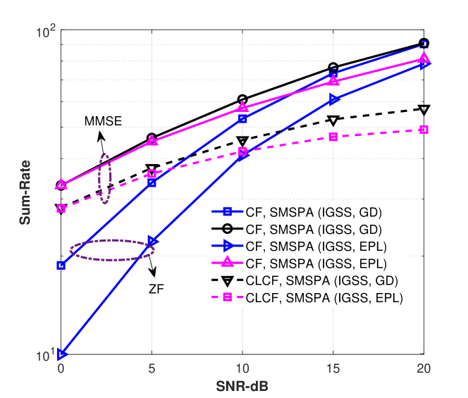
Figure 1: Comparison of the proposed SMSPA technique in CF and CLCF networks with the system that uses the proposed IGSS scheme and EPL for ZF and MMSE precoders, ($M=64$, $K=128$, $n=24$)

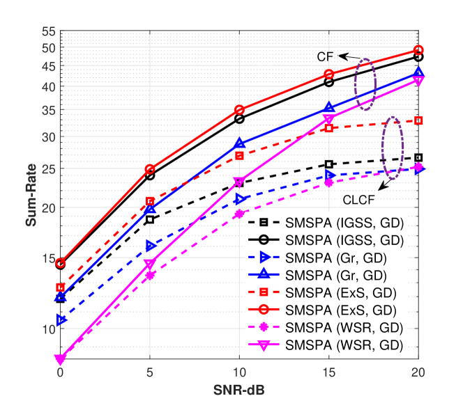
Figure 2: Comparison of different resource allocation techniques considering a GD power allocation algorithm in CF and CLCF networks when an MMSE precoder is used, ($M=64$, $K=16$, $n=8$)

TABLE II: Computational complexity of the proposed resource allocation algorithm and the signaling load for CF and CLCF networks

Network	NO of APs, UEs and scheduled UEs	Signaling load	NO of FLOPs
CF	$M=64$, $K=16$ and $n=8$	3072	$0.78\times 10^{6}$
CLCF	$M=64$, $K=16$ and $n=8$	768	$0.75\times 10^{5}$
CF	$M=128$, $K=256$ and $n=128$	98304	$2.1643\times 10^{10}$
CLCF	$M=128$, $K=256$ and $n=128$	24576	$1.1073\times 10^{9}$

V Conclusion

This paper has developed an SMSPA resource allocation technique for downlink CLCF massive MIMO networks including IGSS multiuser scheduling algorithm which adapts an enhanced greedy technique and a power allocation algorithm which uses a GD method. Simulation results show that the MMSE precoder outperforms ZF and the GD power allocation significantly enhances the sum-rates. It is also shown that the proposed SMSPA technique has better performance than existing methods to a large extent so that the sum-rate performance approaches the optimal exhaustive search. Moreover, the network clustering significantly saves cost and complexity.

References

- [1] H. Q. Ngo, A. Ashikhmin, H. Yang, E. G. Larsson, and T. L. Marzetta, “Cell-free massive mimo: Uniformly great service for everyone,” presented at the IEEE 16th international workshop on SPAWC, Stockholm, Sweden, June. 28th- July. 1st, 2015, pp. 201–205.
- [2] H. Q. Ngo, A. Ashikhmin, H. Yang, E. G. Larsson, and T. L. Marzetta, “Cell-free massive mimo versus small cells,” IEEE Trans. Wirel. Commun., vol. 16, no. 3, pp. 1834–1850, March 2017, doi: 10.1109/TWC.2017.2655515.
- [3] E. Björnson and L. Sanguinetti, “Scalable cell-free massive mimo systems,” IEEE Trans. Commun., vol. 68, no. 7, pp. 4247–4261, July 2020, doi: 10.1109/TCOMM.2020.2987311.
- [4] Ö. T. Demir, E. Björnson, L. Sanguinetti, et al., “Foundations of user-centric cell-free massive mimo,” Found. Trends Signal Process., vol. 14, no. 3-4, pp. 162–472, Jan 2021, doi: 10.1561/2000000109.
- [5] V. Tentu, E. Sharma, D. N. Amudala, and R. Budhiraja, “Uav-enabled hardware-impaired spatially correlated cell-free massive mimo systems: Analysis and energy efficiency optimization,” IEEE Trans. Commun., vol. 70, no. 4, pp. 2722–2741, April 2022, doi: 10.1109/TCOMM.2022.3144470.
- [6] A. P. Guevara, C. M. Chen, A. Chiumento, and S. Pollin, “Partial interference suppression in massive mimo systems: Taxonomy and experimental analysis,” IEEE Access, vol. 9, pp. 128925–128937, 2021, doi: 10.1109/ACCESS.2021.3113167.
- [7] C. Wei, K. Xu, X. Xia, Q. Su, M. Shen, W. Xie, and C. Li, “User-centric access point selection in cell-free massive mimo systems: a game-theoretic approach,” IEEE Commun. Lett., vol. 26, no. 9, pp. 2225–2229, Sept. 2022, doi: 10.1109/LCOMM.2022.3186350.
- [8] Rodrigo C. de Lamare, “Massive mimo systems: Signal processing challenges and future trends,” URSI Radio Science Bulletin, vol. 2013, no. 347, pp. 8–20, 2013.
- [9] Wence Zhang, Hong Ren, Cunhua Pan, Ming Chen, Rodrigo C. de Lamare, Bo Du, and Jianxin Dai, “Large-scale antenna systems with ul/dl hardware mismatch: Achievable rates analysis and calibration,” IEEE Transactions on Communications, vol. 63, no. 4, pp. 1216–1229, 2015.
- [10] Yunlong Cai, Rodrigo C. de Lamare, and Rui Fa, “Switched interleaving techniques with limited feedback for interference mitigation in ds-cdma systems,” IEEE Transactions on Communications, vol. 59, no. 7, pp. 1946–1956, 2011.
- [11] Keke Zu, Rodrigo C. de Lamare, and Martin Haardt, “Generalized design of low-complexity block diagonalization type precoding algorithms for multiuser mimo systems,” IEEE Transactions on Communications, vol. 61, no. 10, pp. 4232–4242, 2013.
- [12] Xiaotao Lu and Rodrigo C. de Lamare, “Opportunistic relaying and jamming based on secrecy-rate maximization for multiuser buffer-aided relay systems,” IEEE Transactions on Vehicular Technology, vol. 69, no. 12, pp. 15269–15283, 2020.
- [13] Yunlong Cai, Rodrigo C. de Lamare, Lie-Liang Yang, and Minjian Zhao, “Robust mmse precoding based on switched relaying and side information for multiuser mimo relay systems,” IEEE Transactions on Vehicular Technology, vol. 64, no. 12, pp. 5677–5687, 2015.
- [14] Hang Ruan and Rodrigo C. de Lamare, “Robust adaptive beamforming using a low-complexity shrinkage-based mismatch estimation algorithm,” IEEE Signal Processing Letters, vol. 21, no. 1, pp. 60–64, 2014.
- [15] Hang Ruan and Rodrigo C. de Lamare, “Robust adaptive beamforming based on low-rank and cross-correlation techniques,” IEEE Transactions on Signal Processing, vol. 64, no. 15, pp. 3919–3932, 2016.
- [16] Jiaqi Gu, Rodrigo C. de Lamare, and Mario Huemer, “Buffer-aided physical-layer network coding with optimal linear code designs for cooperative networks,” IEEE Transactions on Communications, vol. 66, no. 6, pp. 2560–2575, 2018.
- [17] Lukas T. N. Landau and Rodrigo C. de Lamare, “Branch-and-bound precoding for multiuser mimo systems with 1-bit quantization,” IEEE Wireless Communications Letters, vol. 6, no. 6, pp. 770–773, 2017.
- [18] Wence Zhang, Rodrigo C. de Lamare, Cunhua Pan, Ming Chen, Jianxin Dai, Bingyang Wu, and Xu Bao, “Widely linear precoding for large-scale mimo with iqi: Algorithms and performance analysis,” IEEE Transactions on Wireless Communications, vol. 16, no. 5, pp. 3298–3312, 2017.
- [19] Keke Zu, Rodrigo C. de Lamare, and Martin Haardt, “Multi-branch tomlinson-harashima precoding design for mu-mimo systems: Theory and algorithms,” IEEE Transactions on Communications, vol. 62, no. 3, pp. 939–951, 2014.
- [20] Lei Zhang, Yunlong Cai, Rodrigo C. de Lamare, and Minjian Zhao, “Robust multibranch tomlinson–harashima precoding design in amplify-and-forward mimo relay systems,” IEEE Transactions on Communications, vol. 62, no. 10, pp. 3476–3490, 2014.
- [21] Silvio F. B. Pinto and Rodrigo C. de Lamare, “Block diagonalization precoding and power allocation for multiple-antenna systems with coarsely quantized signals,” IEEE Transactions on Communications, vol. 69, no. 10, pp. 6793–6807, 2021.
- [22] Victoria M. T. Palhares, Andre R. Flores, and Rodrigo C. de Lamare, “Robust mmse precoding and power allocation for cell-free massive mimo systems,” IEEE Transactions on Vehicular Technology, vol. 70, no. 5, pp. 5115–5120, 2021.
- [23] Andre R. Flores, Rodrigo C. de Lamare, and Bruno Clerckx, “Linear precoding and stream combining for rate splitting in multiuser mimo systems,” IEEE Communications Letters, vol. 24, no. 4, pp. 890–894, 2020.
- [24] Andre R. Flores, Rodrigo C. De Lamare, and Bruno Clerckx, “Tomlinson-harashima precoded rate-splitting with stream combiners for mu-mimo systems,” IEEE Transactions on Communications, vol. 69, no. 6, pp. 3833–3845, 2021.
- [25] Diana M. V. Melo, Lukas T. N. Landau, Rodrigo C. de Lamare, Peter F. Neuhaus, and Gerhard P. Fettweis, “Zero-crossing precoding techniques for channels with 1-bit temporal oversampling adcs,” IEEE Transactions on Wireless Communications, vol. 22, no. 8, pp. 5321–5336, 2023.
- [26] Patrick Clarke and Rodrigo C. de Lamare, “Joint transmit diversity optimization and relay selection for multi-relay cooperative mimo systems using discrete stochastic algorithms,” IEEE Communications Letters, vol. 15, no. 10, pp. 1035–1037, 2011.
- [27] Patrick Clarke and Rodrigo C. de Lamare, “Transmit diversity and relay selection algorithms for multirelay cooperative mimo systems,” IEEE Transactions on Vehicular Technology, vol. 61, no. 3, pp. 1084–1098, 2012.
- [28] Yuhan Jiang, Yulong Zou, Haiyan Guo, Theodoros A. Tsiftsis, Manav R. Bhatnagar, Rodrigo C. de Lamare, and Yu-Dong Yao, “Joint power and bandwidth allocation for energy-efficient heterogeneous cellular networks,” IEEE Transactions on Communications, vol. 67, no. 9, pp. 6168–6178, 2019.
- [29] Hang Ruan and Rodrigo C. de Lamare, “Distributed robust beamforming based on low-rank and cross-correlation techniques: Design and analysis,” IEEE Transactions on Signal Processing, vol. 67, no. 24, pp. 6411–6423, 2019.
- [30] André R. Flores and Rodrigo C. de Lamare, “Robust and adaptive power allocation techniques for rate splitting based mu-mimo systems,” IEEE Transactions on Communications, vol. 70, no. 7, pp. 4656–4670, 2022.
- [31] G. Interdonato, E. Björnson, H. Quoc Ngo, P. Frenger, and E. G. Larsson, “Ubiquitous cell-free massive mimo communications,” Eurasip J. Wirel. Commun. Netw., vol. 2019, no. 1, pp. 1–13, Aug. 2019, doi: 10.1186/s13638-019-1507-0.
- [32] S. Mosleh, H. Almosa, E. Perrins, and L. Liu, “Downlink resource allocation in cell-free massive mimo systems,” presented at the ICNC, Honolulu, Hawaii, USA, Feb. 18-21, 2019, pp. 883–887.
- [33] S. Wu, L. Liu, W. Zhang, W. Meng, Q. Ye, and Y. Ma, “Revenue-maximizing resource allocation for multitenant cell-free massive mimo networks,” IEEE Systems Journal, vol. 16, no. 2, pp. 3410–3421, June 2022, doi: 10.1109/JSYST.2021.3072419.
- [34] H. A. Ammar, R. Adve, S. Shahbazpanahi, G. Boudreau, and K. V. Srinivas, “Downlink resource allocation in multiuser cell-free mimo networks with user-centric clustering,” IEEE Trans. Wireless Commun., vol. 21, no. 3, pp. 1482–1497, March 2022, doi: 10.1109/TWC.2021.3104456.
- [35] S. Mashdour, R. C. de Lamare, and J. P. S. H. Lima, “Multiuser scheduling with enhanced greedy techniques for multicell and cell-free massive mimo systems,” presented at the IEEE 95th VTC, Helsinki, Finland, June. 19-22, 2022, pp. 1–5.
- [36] A. Tang, J. Sun, and K. Gong, “Mobile propagation loss with a low base station antenna for nlos street microcells in urban area,” presented at the IEEE VTS 53rd VTC, Rhodes, Greece, May. 6-9, 2001, pp. 333–336.
- [37] Rodrigo C. de Lamare and Raimundo Sampaio-Neto, “Adaptive reduced-rank processing based on joint and iterative interpolation, decimation, and filtering,” IEEE Transactions on Signal Processing, vol. 57, no. 7, pp. 2503–2514, 2009.
- [38] Rodrigo C. De Lamare and Raimundo Sampaio-Neto, “Minimum mean-squared error iterative successive parallel arbitrated decision feedback detectors for ds-cdma systems,” IEEE Transactions on Communications, vol. 56, no. 5, pp. 778–789, 2008.
- [39] Peng Li, Rodrigo C. de Lamare, and Rui Fa, “Multiple feedback successive interference cancellation detection for multiuser mimo systems,” IEEE Transactions on Wireless Communications, vol. 10, no. 8, pp. 2434–2439, 2011.
- [40] Rodrigo C. de Lamare, “Adaptive and iterative multi-branch mmse decision feedback detection algorithms for multi-antenna systems,” IEEE Transactions on Wireless Communications, vol. 12, no. 10, pp. 5294–5308, 2013.
- [41] Andre G. D. Uchoa, Cornelius T. Healy, and Rodrigo C. de Lamare, “Iterative detection and decoding algorithms for mimo systems in block-fading channels using ldpc codes,” IEEE Transactions on Vehicular Technology, vol. 65, no. 4, pp. 2735–2741, 2016.
- [42] Lukas T. N. Landau, Meik Dörpinghaus, Rodrigo C. de Lamare, and Gerhard P. Fettweis, “Achievable rate with 1-bit quantization and oversampling using continuous phase modulation-based sequences,” IEEE Transactions on Wireless Communications, vol. 17, no. 10, pp. 7080–7095, 2018.
- [43] Zhichao Shao, Lukas T. N. Landau, and Rodrigo C. de Lamare, “Dynamic oversampling for 1-bit adcs in large-scale multiple-antenna systems,” IEEE Transactions on Communications, vol. 69, no. 5, pp. 3423–3435, 2021.
- [44] S. Mashdour, R. C. De Lamare, and J. P. S. H. Lima, “Enhanced subset greedy multiuser scheduling in clustered cell-free massive mimo systems,” IEEE Commun. Lett., 2022, doi: 10.1109/LCOMM.2022.3230641.
- [45] S. Verdu et al., Multiuser detection, Cambridge university press, 1998.
- [46] G. Dimic and N. D. Sidiropoulos, “On downlink beamforming with greedy user selection: performance analysis and a simple new algorithm,” IEEE Trans. Signal Process., vol. 53, no. 10, pp. 3857–3868, Oct. 2005, doi: 10.1109/TSP.2005.855401.