Semi-metric topology characterizes epidemic spreading on complex networks

Abstract

Network sparsification represents an essential tool to extract the core of interactions sustaining both networks dynamics and their connectedness. In the case of infectious diseases, network sparsification methods remove irrelevant connections to unveil the primary subgraph driving the unfolding of epidemic outbreaks in real networks. In this paper, we explore the features determining whether the metric backbone, a subgraph capturing the structure of shortest paths across a network, allows reconstructing epidemic outbreaks. We find that both the relative size of the metric backbone, capturing the fraction of edges kept in such structure, and the distortion of semi-metric edges, quantifying how far those edges not included in the metric backbone are from their associated shortest path, shape the retrieval of Susceptible-Infected (SI) dynamics. We propose a new method to progressively dismantle networks relying on the semi-metric edge distortion, removing first those connections farther from those included in the metric backbone, i.e. those with highest semi-metric distortion values. We apply our method in both synthetic and real networks, finding that semi-metric distortion provides solid ground to preserve spreading dynamics and connectedness while sparsifying networks.

I Introduction

The advent of network epidemiology in the XXI century Keeling and Eames (2005); Morris (2004) has fueled our knowledge about how epidemic outbreaks unfold across real interconnected societies. The increasing relevance of this field for disease control Metcalf et al. (2020); Pagel and Yates (2022) has been prompted by the availability of realistic networks characterizing our interactions across multiple scales Blondel et al. (2015); Stehlé et al. (2011). Indeed, the sole structural characterization of high resolution spatio-temporal networks provides insightful information to face an epidemic outbreak. For instance, the analysis of mobility networks has shed light into diverse problems such as the risk of importing cases from sources of contagions worldwide Gilbert et al. (2020); Brockmann and Helbing (2013) or the heterogeneous community transmission observed across a given country Hazarie et al. (2021). Likewise, the existence of high resolution datasets has spurred the quest for new theories that incorporate the complex nature of human interactions. Consequently, different layers of complexity have been added to the originally proposed mean-field theories, resulting in more sophisticated mathematical models such as the heterogeneous mean-field (HMF) theory Pastor-Satorras and Vespignani (2001); Gómez et al. (2011), the Microscopic Markov Chain Approach (MMCA) Gómez et al. (2010) or the pair-quenched mean field approach (PQMF) Mata and Ferreira (2013); Silva et al. (2020) among others Wang et al. (2017). Those developments have improved the forecastability of epidemic models and their use as reliable benchmarks to assess the short-term impact of control policies Shea et al. (2023).

One of the recurrent problems tackled by network epidemiology is the design of optimal interventions to mitigate an epidemic outbreak while minimally disrupting the underlying network structure Meyers et al. (2003); Della Rossa et al. (2020). One type of such interventions is to isolate those agents driving the spread of a virus. For this purpose, one usually relies on node centrality measures to control the outbreak, determining for instance those individuals which should be first vaccinated when facing an epidemic Rosenblatt et al. (2020); Mones et al. (2018); Wei et al. (2022) or those geographical areas which should be prioritized in the spatial distribution of resources Reyna-Lara et al. (2022); Ndeffo Mbah and Gilligan (2011); Zhu et al. (2021). Beyond structural properties, nodes isolation policies might be also guided by dynamical information, as recently proven in the context of COVID-19 pandemic with the efficient quarantine of potentially infectious individuals following contact tracing information Reyna-Lara et al. (2021); Bassolas et al. (2022); Kojaku et al. (2021). Another family of interventions targets nodes’ interactions by reshuffling certain edges or removing specific connections Ciaperoni et al. (2020) to protect the population from the spread of a circulating pathogen. The latter strategies are usually driven either by edge-centrality measures Wen et al. (2017); Chung et al. (2012); Liang et al. (2023), which might incorporate just structural information of the underlying network, e.g. edge betweenness, or also account for the dynamical state of the system, e.g. the link importance defined in Matamalas et al. (2018).

Removing network connections which hardly influence the spreading dynamics also constitutes another important challenge in the Big Data era. Specifically, this problem aims at pruning a large set of redundant connections which are usually present in high resolution databases and play a minor role in the spreading dynamics across the network. Therefore, the sparsification of contact networks allows unveiling the primary subgraphs sustaining the spread of a pathogen and simultaneously reducing the computational cost of spreading dynamics’ simulations. Several network sparsification methods Serrano et al. (2009); Tumminello et al. (2005) have been developed over the last decades to hamper redundancy in networks, differing from one another in the measures used to determine the removal of each edge in the network. These measures can be assigned following local information Yan et al. (2018), the statistical significance of a given connection Radicchi et al. (2011); Marcaccioli and Livan (2019); Gemmetto et al. (2017), or accounting for the impact of edge removal on different network properties such as the spectrum of their different mathematical representations Imre et al. (2020); Bravo Hermsdorff and Gunderson (2019) or their global structure of paths Spielman and Srivastava (2008); Simas et al. (2021). Other methods have also been proposed to reduce the network size through effective renormalization groups Wilson and Kogut (1974), based on either its embedding in hyperbolic spaces García-Pérez et al. (2018) or the properties of its associated Laplacian graph Villegas et al. (2023).

The interplay between network sparsification and spreading dynamics has received much less attention than the design of targeted strategies to control an outbreak. Mounting evidence in the literature suggests that network sparsification relying on global information allows for a better retrieval of spreading dynamics than just removing the weakest connections. For instance, sparsifying the network according to the distribution of effective resistance values, which account for the relevance of a given edge within the ensemble of paths connecting their two nodes, outperforms weights thresholding in preserving both SI Swarup et al. (2016) and SIR Mercier et al. (2022) dynamics. Along the same line, the study of spreading phenomena through shortest paths in a network has been used to address different problems such as the inference of the source of an outbreak Tolić et al. (2018) or the expected distribution for the arrival times of the pathogen to different locations Gautreau et al. (2007). Following this spirit, a recent paper published by Correia et al. Brattig Correia et al. (2023) shows that the metric backbone—a unique and algebraically-principled subgraph that preserves the entire distribution of shortest-paths of a weighted graph— provides more solid foundations for network sparsification than relying on local information.

Despite previous studies on the relevance of the metric backbone Simas and Rocha (2015); Brattig Correia et al. (2023), determining the network features limiting the reconstruction of epidemic outbreaks from the struc ture of shortest paths in a given network remains an open problem. In this paper, we tackle this challenge and reveal that the former reconstruction crucially hinges on the properties of the semi-metric edges, i.e. those connections not belonging to the metric backbone and, therefore, not participating in any shortest path in the network. In particular, we show that this process is shaped by the interplay between the number of semi-metric edges, determining the potential transmission pathways missed in the metric backbone, and their associated semi-metric distortion $s^{m}$ Simas et al. (2021), quantifying how far they are from the indirect shortest path connecting their nodes. The latter result allow us to propose a new sparsification method following the distribution of semi-distortion values, removing first those more apart from the shortest paths in the network. We prove that, for both synthetic and real networks, the semi-metric distortion sparsification outperforms other methods studied in the literature in retrieving the underlying spreading dynamics and ensuring the network connectedness. Our results prove that studying the structure of shortest paths reveals primary subgraphs for spreading dynamics and provide useful guidance to identify the subset of connections which should be targeted to effectively mitigate epidemic outbreaks.

II Results

II.1 Interplay between SI dynamics and metric backbone

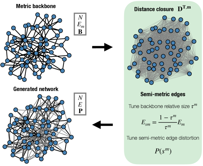
Figure 1: Schematic representation of the construction of synthetic networks with tunable relative size of the backbone $\tau^{m}$ and semi-metric distortion distribution $P(s^{m})$. The first step consists of setting the metric backbone of the synthetic network. This metric backbone is fully characterized by the number of nodes $N$, the number of edges $E_{m}$ and the proximity matrix ${\bf B}$ containing the weights of interactions. The next step involves computing the distance closure matrix ${\bf D^{T,m}}$, a fully-connected graph containing the length of the shortest paths connecting every pair of nodes. Finally, we generate the synthetic network by adding $E_{sm}$ edges, whose value is computed according to Eq. (7) in the Methods sections, to obtain a given relative backbone size $\tau^{m}$. The semi-metric distortion values of the added edge $s_{ij}^{m}$ are drawn from the target distribution $P(s^{m})$. Finally, the resulting proximity matrix ${\bf P}$ is obtained by applying Eqs. (5) and (3) of the Methods section to each $s^{m}_{ij}$ value.

We first explore different network features shaping outbreaks reconstruction from the collections of edges participating in shortest paths and, therefore, captured in the metric backbone. To address this challenge, we propose a new method, schematized in Figure 1, to construct synthetic networks where we can tune the relative size of the metric backbone $\tau^{m}$ and the distribution of semi-metric distortion values $P(s^{m})$, which is . We refer the reader to the Methods section for a complete explanation of the theoretical foundations of the metric backbone and the semi-metric edge distortion. Starting from a metric backbone of $N$ nodes and $E_{m}$ edges, our method adds semi-metric connections to build a network of $N$ nodes and $E$ edges, whose strength of interactions are quantified in the proximity matrix ${\bf P}$. A detailed description of our method to construct synthetic networks is provided in the Methods section.

To focus on the role of the aforementioned features, $\tau^{m}$ and $P(s^{m})$, while preserving other empirically relevant structures, the synthetic networks are built from the backbone of a real network. Specifically, we utilize the backbone of a contact network between elementary school students (kindergarten to sixth grade) in Utah (USA) Toth et al. (2015); Brattig Correia et al. (2023). This network is composed of $N=339$ nodes and $E_{m}=1128$ metric edges, with a heterogeneous distribution of the proximity values (available in Figure S1 in the Supplementary text). Moreover, semi-metric distortion values are drawn from a log-normal distribution, i.e. $s^{m}\sim Lognormal(\mu,\sigma)$, since this probability function is widespread across different empirical networks Simas et al. (2021); Brattig Correia et al. (2023). Throughout the manuscript, we fix $\sigma=1$ and modify the $\mu$ value to study the effect of semi-metric edges’ relevance with respect to those included in the metric backbone.

To assess how these features limit the reconstruction of outbreaks from the metric backbone, we introduce a single infectious seed, i.e. a single individual initially infected, and run a SI dynamics, obtaining the time at which half of the population was infected in both the metric backbone and the entire network, denoted by $t^{B(X)}_{1/2}$ and $t_{1/2}$ respectively. Further details on the SI model and the chosen parameters can be found in the Methods section. To quantify the extent to which the metric backbone preserves SI dynamics given an initial infectious seed, we compute the ratio between the former quantities, yielding:

$$\xi^{B(X)}_{1/2}=\frac{t_{1/2}^{B(X)}}{t_{1/2}}\ .$$ (1)

In absence of stochastic fluctuations, the aforementioned ratio fulfills $\xi^{B(X)}_{1/2}\geq 1$, as the metric backbone always removes potential transmission pathways for the virus existing in the original network. In terms of performance, the closer this ratio gets to $\xi^{B(X)}_{1/2}=1$, the more faithful the information provided by the metric backbone is about the dynamics in the entire network.

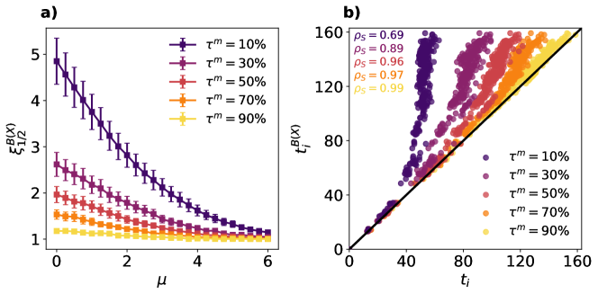
Figure 2: Panel a): Ratio between the time for the disease to reach half the population in the metric backbone and in the constructed network $\xi_{1/2}^{B(X)}$ as a function of the parameter $\mu$, i.e. the logarithm of the median of the semi-metric distortion distribution, and the relative size of the backbone $\tau^{m}$ (color code). For a given seed, we compute the time to reach half the population $t_{1/2}$ as the median value observed across $200$ realizations of the SI dynamics. Dots show the average and error bars represent the standard deviation of the ratios obtained for $50$ different infectious seeds. Panel b): Average time of infection of each individual $i$ in the metric backbone $t_{i}^{B(X)}$ as a function of its average time of infection in the entire network $t_{i}$ for different values of the relative size of the backbone $\tau^{m}$ (color code). These results are obtained by averaging $200$ realizations starting from the same initial seed. In both panels, we set $\beta=0.5$ for the SI dynamics, fix $\sigma=1$ in the semi-metric distortion distribution and consider the metric backbone ${\bf B}$ of a network capturing face-to-face interactions in a elementary school in the US Toth et al. (2015).

Figure  2a represents the ratio $\xi^{B(X)}_{1/2}$ as a function of the semi-metric edges relevance, governed by $\mu$, and the relative size of the backbone $\tau^{m}$. For large $\mu$ values, semi-metric edges are highly dynamically redundant in comparison with the metric ones as $\xi^{B(X)}_{1/2}\simeq 1$ regardless of the backbone relative size. Therefore, their removal hardly has any influence on the spreading. As edges distances become closer to the shortest path lengths, we observe a critical value $\mu_{c}$ for each $\tau^{m}$ value below which the spreading dynamics gets slower in the metric backbone ($\xi^{B(X)}_{1/2}>1$). Interestingly, this critical value $\mu_{c}$ increases as the size of the backbone decreases. The latter results imply that the performance of the metric backbone is determined by the interplay between both the potential transmission pathways pruned during the sparsification process (governed by $\tau^{m}$) and their relevance with respect to those kept there (the semi-metric distortion, governed by $\mu$).

The previous results show that considering the metric backbone as the underlying contact structure might induce global delays in the spreading dynamics. Nonetheless, even in those scenarios, the information obtained from this subgraph can be relevant for disease control if the metric backbone allows us to faithfully rank the different nodes according to their expected time of infection. To check that, we randomly place a single infectious seed in the network and study how the distribution of the individual infection times varies as we alter the properties of the metric backbone. In particular, we fix $\mu=2$ and explore the role of the relative size of the backbone $\tau^{m}$ in the microscopic reconstruction of outbreaks. Figure  2b shows that, even when the metric backbone represents just $10\%$ of the edges of the network, it qualitatively captures the epidemic trajectory across the population, as shown by the high Spearman correlation between the distributions obtained for both the network and its backbone ($\rho_{S}=0.69$, $p<0.001$). As expected, the microscopic retrieval of the epidemic trajectory is also enhanced as $\tau^{m}$ increases and more transmission pathways are captured in the metric backbone.

II.2 Semi-metric distortion sparsification in synthetic networks

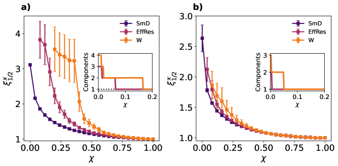
Figure 3: Ratio between the time for the disease to reach half the population in the sparsified network and in the original synthetic network $\xi^{x}_{1/2}$ as function of the parameter governing the size of the sparsified network $\chi$ for each sparsification method $x$ (color code). $\chi$ ranges from $\chi=1$, corresponding to not removing any edge, to $\chi=0$ where $E_{sm}$ edges are removed. Three different sparsification methods are compared: targetting edges with highest semi-metric distortion values (SmD), lowest effective resistance values (EffRes) or lowest proximity values (W). The details of the simulations to obtain the ratios are the ones described for Figure 2A. EffRes and W curves are interrupted when breaking the largest connected component of the network. Insets: Number of components in the network as a function of the edges removed $\chi$ and the sparsification method (color code). The horizontal dashed line represents the semi-metric distortion sparsification, which always preserves the largest connected component. The original synthetic networks are constructed as detailed in Section IV.2 considering $\tau^{m}=0.1$ and $\mu=1$ (Panel a) or $\mu=2$ (Panel b) respectively.

Our findings indicate that the removal of semi-metric edges with large $s^{m}$ values hardly affects the outcome of SI dynamics, thus making them dynamically redundant. Motivated by this result, here we propose a new sparsification method to progressively dismantle a network relying on the distribution of semi-metric distortion values $s^{m}$. To sparsify the network, we sort the edges $(i,j)$ according to their associated distortion values $s_{ij}^{m}$ and remove those with highest distortion values until matching the desired size of the sparsified configuration. Note that this sparsification method is deterministic, hereinafter referred to as semi-metric distortion thresholding, yielding a single network trajectory from the entire network to the metric backbone. This choice allows for removing the stochasticity associated to edge sampling when pruning the network based on edge removal probabilities. We compare the method proposed here with two sparsification schemes relying on different edges properties: weights thresholding and effective resistance thresholding. On the one hand, weights thresholding relies on local information, aiming at removing the weakest connections through which transmission of the virus is very unlikely. On the other hand, effective resistance thresholding penalizes path redundancy, as small effective resistance values identify those direct edges connecting nodes which can also exchange information through many other indirect paths. More details on the computation of the effective resistance associated to each edge can be found in the Methods section.

To compare the three sparsification methods, we compute the evolution of the ratio $\xi^{x}_{1/2}(\chi)=t^{x}_{1/2}(\chi)/t_{1/2}$ for each subgraph obtained after removing edges according to each sparsification method $x$. For the semi-metric distortion thresholding, the parameter $\chi$ encodes the fraction of semi-metric edges included in the network, i.e. $E(\chi)=E_{m}+\chi E_{sm}$. Therefore, $\chi=1$ corresponds to the entire synthetic network whereas $\chi=0$ corresponds to just keeping the metric backbone in the sparsified configuration. For the other two processes, the sparsified networks comprise $E(\chi)$ edges which are chosen following the distribution of weights $p_{ij}$ or effective resistance $p^{R}_{ij}$ values respectively.

Figure 3a shows the comparison of the three sparsification methods in a synthetic network with $\tau^{m}=0.1$ and $\mu=1$. There we observe that semi-metric distortion thresholding outperforms the other two methods in both preserving SI dynamics and keeping the connectedness of the network. Specifically, the curves following semi-metric distortion fall closer to $\xi_{1/2}\simeq 1$, implying that accounting for the edge relevance with respect to their associated shortest path during sparsification helps reconstruct the spreading dynamics. Moreover, semi-metric distortion thresholding does not target any metric edge by definition and therefore guarantees the existence of at least one path connecting every pair of nodes. In contrast, the other two methods eventually dismantle the largest connected component, breaking the network into different subgraphs. Note that this phenomenon is more pronounced for weights thresholding, as effective resistance thresholding harnesses global information and makes the isolation of individual nodes more difficult.

Remarkably, increasing $\mu$ in the synthetic network shrinks the differences between these three methods, as shown in Figure 3b when we construct the network by fixing $\mu=2$. In this case, semi-metric edges are far from the shortest path, thus making both weights and effective resistance thresholding less likely to target the metric backbone, as shown in Figure S2 in the Supplementary text. The previous result supports the role of the metric backbone as a primary subgraph sustaining the spread of diseases Brattig Correia et al. (2023).

II.3 Semi-metric distortion sparsification in empirical networks

To further support our claims, we also consider a dataset of 16 empirical networks comprising different biological, social and mobility graphs. We refer the reader to the Methods section for further information about the construction of these networks, whose structural features are summarized in Table S1 in the Supplementary text. The individual curves for each of these networks comparing the three sparsification methods can be found in Figure S3 in the Supplementary text. For the sake of illustration, we represent in Figure 4a the one corresponding to the network capturing face-to-face interactions in the US elementary school. There we observe that semi-metric distortion sparsification presents the same advantages as the ones discussed before for synthetic networks, i.e. better retrieval of SI dynamics and no disruption of the largest connected component of the network.

Figure 4: Panel a): Ratio between the time for the disease to reach half the population in the sparsified network and in the original synthetic network $\xi^{x}_{1/2}$ as a function of the parameter $\chi$, governing the edges removed from the network, and the sparsification method $x$ (color code). The contact network corresponds to face-to-face interactions recorded in an elementary school students (kindergarten to sixth grade) in Utah (USA) Toth et al. (2015). The details of the simulations to obtain the ratios are the ones described for Figure 2A. Panel b): Distribution of the relative difference $\tilde{\Delta\xi}^{x}_{1/2}$ between the mean ratio associated to each sparsification method $x$ (color code) and the one following semi-metric distortion as a function of the size of the sparsified network $\chi$. Positive $\tilde{\Delta\xi}^{x}_{1/2}$ values reveal a better performance of the networks sparsified following semi-metric distortion with respect to the sparsification method $x$. Dots represent each of the 16 networks included in the dataset under study whereas solid lines show the median $\tilde{\Delta\xi}_{1/2}^{x}$ value observed across networks for each sparsification method $x$. Panel c): Fraction of disconnected networks in the dataset of real networks $f^{x}$ as a function of the size of the sparsified network $\chi$ and the sparsification method $x$ (color code). In both panels, the horizontal dashed line represents the values obtained for the semi-metric distortion sparsification.

To quantify the better retrieval of SI dynamics by following semi-metric distortion in empirical networks, we compute how the relative differences $\tilde{\Delta\xi}_{1/2}^{x}$ between the mean ratios found in the semi-metric distortion sparsification and each method $x$ varies as a function of the size of the network $\chi$. For a given size of the sparsified network $\chi$ and a given sparsification method $x$, where $x$ stands for either weights or effective resistance thresholding, this relative difference reads:

$$\tilde{\Delta\xi}^{x}_{1/2}(\chi)=\frac{\xi^{x}_{1/2}(\chi)-\xi^{SmD}_{1/2}(\chi)}{\xi^{SmD}_{1/2}(\chi)}\ .$$ (2)

Therefore, $\tilde{\Delta\xi}^{x}_{1/2}>0$ implies that semi-metric distortion outperforms the sparsification method $x$. As in the synthetic networks, Figure 4b shows little-to-no differences across sparsification methods when removing few connections from the network, as $\xi^{x}_{1/2}\simeq 1$ when $\chi\simeq 1$ regardless of the method considered . Nonetheless, as more links get pruned, semi-metric distortion thresholding typically outperforms the other two methods as shown by the positive median of the distribution of ${\Delta\xi}^{x}_{1/2}$ values obtained for the different networks in the dataset. Note that, however, there are some networks for which ${\Delta\xi}^{x}_{1/2}<0$, meaning that following semi-metric distortion does not constitute the best strategy to simplify the network when preserving SI dynamics. To further support our findings, we represent in Figure S4 in the Supplementary text the comparison between the three methods for different stages of the outbreak. There we observe that semi-metric distortion sparsification generally allows for a better construction of the dynamics except for early stages of the epidemic spreading, when only $10\%$ of the population has been infected. In that case, the set of infected individuals reflects the composition of very localized epidemic states around the infectious seed, thus making the global information encoded in the semi-metric distortion values less relevant.

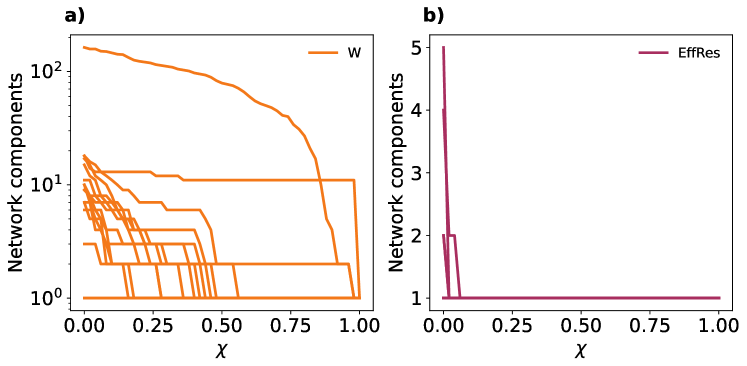
Figure S5: Number of connected components for the empirical networks as a function of the size of the sparsified network $\chi$. $\chi$=1 preserves all the connections in the network whereas $\chi=0$ corresponds to networks whose number of connections matches the size of the metric backbone.

To round off our analysis, for each sparsification method $x$, we represent in Figure 4c the fraction of disconnected networks $f^{x}$ across the set of empirical graphs as a function of the size of the network. In this plot, we observe that networks are quite vulnerable to weights thresholding, as most of the networks in our dataset eventually break into different components. In the case of effective resistance thresholding, yet more resilient due to the global information encoded in the effective resistance, 4 out of 16 networks end up breaking when removing the same number of edges as semi-metric connections in the network ($\chi=0$). To complete this picture, Figure S5 in the Supplementary text represents the evolution of the number of components as a function of the size $\chi$ for the different networks here studied, showing that the way in which these sparsification methods dismantle networks is not universal but highly dependent on the specific architecture of each graph.

III Discussion

Nowadays, the existence of sophisticated data gathering techniques allows obtaining an accurate representation of interactions spanning multiple scales in nature, ranging from biological networks obtained at the organism level to contact structures or mobility networks determining our social interactions. Despite the data-driven scientific progress in these fields prompted by the so-called Big Data era, current datasets usually include residual links not contributing to the backbone of interactions governing the dynamics of these systems Mercier et al. (2022). These residual interactions enlarge considerably the networks, blurring the information provided by their visualization and stressing the computational issues inherent to both their storage and analysis. The former caveats make network sparsification tools essential to leverage the high spatiotemporal resolution of current datasets while minimizing the aforementioned side effects associated with the large data availability.

In this work, we have investigated whether the structure of shortest paths provides reliable guidance for sparsifying a network while preserving spreading dynamics. To do so, first we have studied the network features determining the reconstruction of SI outbreaks from the metric backbone, constructed by the subset of edges that participate in shortest paths in the network. Our results highlights that the reconstruction of outbreaks is shaped by a nontrivial interplay between the quantity and quality of the edges missed in the metric backbone. Namely, removing edges that are very far from the shortest connection hardly affects the dynamics regardless of the relative size of the backbone. On the contrary, the amount of edges pruned when getting the backbone gains relevance for connections closer to the shortest path length, as a consequence of the potential transmission pathways blocked for the pathogen. Nonetheless, yet inducing a global delay in the spreading dynamics, the metric backbone faithfully classify nodes according to their exposure to the outbreak, thus providing useful information for the prioritization of individual control strategies.

The previous results indicate that edge relevance compared to the structure of shortest paths plays a crucial role in the reconstruction of spreading phenomena. Such relevance can be quantified by the semi-metric distortion value, measuring how longer the direct edge between two nodes is with respect to the shortest path connecting them. Based on the previous result, we have proposed a new sparsification method to progressively dismantle the network by removing those connections with highest semi-metric distortion values. We have compared this method with both weights thresholding, a local sparsification method targeting the weakest connections, and effective resistance thresholding, a global sparsification method penalizing the existence of multiple paths connecting two nodes. Our results indicate that relying on semi-metric distortion not only allows for a better retrieval of the dynamics but also ensures network functionality by not breaking the largest connected component of the network. From a broader perspective, the prominent role of semi-metric edges, with zero edge betweenness by definition, calls for new edge centrality measures, incorporating not only the edges’ participation but also their relation to shortest paths in the networks.

Taken together, our findings indicate that the structure of shortest paths in the network along with the information about the distortion of semi-metric edges provides solid ground for network sparsification. Note, however, that the results here discussed are restricted to the application of metric distances to SI dynamics. Due to the nature of this compartmental model, the emergence of a global infected configuration is guaranteed and shortest paths appear as a natural driver for contagion processes. Other compartmental models, such as the Susceptible-Infected-Susceptible (SIS) or the Susceptible-Infected-Recovered (SIR) models, usually display localized epidemic outbreaks Silva and Ferreira (2021); Cota et al. (2016), in which the prevalence of global information over local weights for network sparsification remains an open question. Likewise, the structure of shortest metric paths has been reported not to capture other diffusion processes, such as random walker dynamics, which are better represented by longer but more likely network bypasses governing the flow of information across the network Estrada et al. (2023); Lella and Estrada (2020). Far from being limitations, the former issues demand going beyond the metric space and including tailored backbones Simas and Rocha (2015) capturing the specific nature of the analyzed dynamics. We hope that both the methodology presented here and our results further motivate the quest for dynamical backbones governing different processes on networks.

IV Methods

IV.1 Metric backbone and semi-metric distortion

Here we give a brief overview about the theoretical foundations of the metric backbone and the semi-metric edge distortion. Let us assume that we have a system of $N$ individuals whose interactions are encoded in a proximity matrix ${\bf P}$, with elements $p_{ij}$ denoting the strength of the interaction existing between nodes $i$ and $j$. Obtaining the metric backbone involves the computation of shortest paths in the network; thus, we need a map between the proximity matrix ${\bf P}$ and the distance matrix ${\bf D}$. The elements of the latter matrix, $d_{ij}$, represent a notion of distance between nodes $i$ and $j$, such that a stronger connection means that the nodes are closer. A possible choice is:

$$d_{ij}=\frac{1}{p_{ij}}-1\ ,$$ (3)

with $d_{ij}\to\infty$ in case two nodes do not interact. Other choices would correspond to different backbones Simas and Rocha (2015), which are to be considered in future work. Once defined the individual distances, we compute the metric distance of a given path $\Gamma=\quantity{i,k_{1},\dots,k_{n},j}$ connecting two nodes $i$ and $j$ as

$$d_{ij}(\Gamma)=d_{ik_{1}}+d_{k_{1}k_{2}}+\dots+d_{k_{n}j}\ ,$$ (4)

where $n$ stands for the number of intermediate nodes in the path. The shortest path length connecting both nodes, denoted by $d_{ij}^{T,m}$, is thus computed as $d^{T,m}_{ij}=\min_{\Gamma}\quantity(\quantity{d_{ij}(\Gamma)})$, which by construction satisfies $d_{ij}^{T,m}\leq d_{ij}$. The collection of shortest path distances is encoded in the metric closure matrix, denoted by ${\bf D^{T,m}}$. Comparing these values with the matrix ${\bf D}$, we can quantify the edge distortion $s_{ij}^{m}$, measuring how far a given connection between two nodes $i$ and $j$ is from the shortest path length connecting them:

$$s_{ij}^{m}=\frac{d_{ij}}{d^{T,m}_{ij}}\ .$$ (5)

Therefore, a direct edge $(i,j)$ constituting the shortest path between nodes $i$ and $j$ satisfies $s_{ij}^{m}=1$ and is referred to as metric edge; otherwise, $s_{ij}^{m}>1$ and the edge is called semi-metric. Consequently, the metric edges are those with non-zero betweenness centrality in the network. The set of metric edges defines the metric backbone ${\bf B}$, whose relative size $\tau^{m}$ is given by

$$\tau^{m}=\frac{\absolutevalue{\{d_{ij}<\infty:d_{ij}=d_{ij}^{T}\}}}{\absolutevalue{\{d_{ij}<\infty\}}},$$ (6)

measuring the proportion of edges kept in this subgraph and, therefore, participating in shortest paths across the network. For unweighted graphs, the relative size of the metric backbone is $\tau^{m}=1$, as all the direct edges represent the shortest path between their nodes. In contrast, for weighted graphs, this relative size varies across networks, depending on both the weights distribution and the specific structure of paths in each graph. The metric backbone is just one of the backbones which can be extracted from the distance matrix ${\bf D}$, according to how the length of a path is measured and how the different paths are combined. While in this work we are exclusively interested in the metric backbone, we refer the reader to Simas et al. (2021) for a more exhaustive exploration of other backbones and their properties.

IV.2 Construction of synthetic networks

The first step to construct the synthetic networks used in this manuscript is to fix their metric backbone. To do so, we consider an undirected weighted network with $N$ nodes and $E_{m}$ edges, whose proximity values are captured in the matrix ${\bf B}$. This initial subgraph has to satisfy all the constraints characterizing the metric backbone of a given network. Namely, it must have a single connected component and all its edges must be metric, i.e. they must represent the shortest path connecting their nodes. The next step involves mapping the proximity values to distances via Eq. (3) and computing the metric closure matrix ${\bf D^{T,m}}$, thus obtaining the length of the shortest path connecting every pair of nodes in the network. Note that our method does not alter the structure of shortest paths in the network; therefore ${\bf D^{T,m}}$ constitutes the metric closure matrix of the final synthetic network.

On top of the metric backbone, we add $E_{sm}$ edges to tune its relative size $\tau^{m}$ compared to the total size of the constructed network. If $E=E_{m}+E_{sm}$ denotes the total number of edges in the constructed network, the relative size fulfills $E_{m}=\tau^{m}E$. Therefore, to fix a specific value $\tau^{m}$, the number of semi-metric edges to be added is:

$$E_{sm}=\frac{1-\tau^{m}}{\tau^{m}}E_{m}\ .$$ (7)

These $E_{sm}$ edges are chosen randomly within the set of edges not present in the metric backbone B. Note that $\tau^{m}\in\left[\frac{2E_{m}}{N(N-1)},1\right]$, where the lower bound corresponds to including all missing semi-metric edges to obtain a fully-connected network.

Once we fix the relative size of the backbone, we move to tuning the distortion of the semi-metric edges in the network. To do so, for each added edge, we sample its semi-metric distortion value $s_{ij}^{m}$ from the target distribution $P(s^{m})$ and assign the individual distance $d_{ij}$ of the new link following Eq. (5). Therefore,

$$d_{ij}=s_{ij}^{m}d^{T,m}_{ij}\ ,$$ (8)

which are eventually transformed into proximity values by using Eq. (3), yielding:

$$p_{ij}=\left(d_{ij}+1\right)^{-1}\ .$$ (9)

IV.3 SI dynamics

We focus on the the Susceptible-Infected (SI) compartmental model as a proxy for spreading dynamics due to its simplicity. In the SI model, there are only two states (compartments) available for each individual: Susceptible and Infected. A susceptible host $i$ contracts a virus and becomes infected when interacting with one infectious counterpart $j$ at a rate $\beta p_{ji}$. Once nodes are infected, they remain in this state over the entire dynamics. Therefore, the SI dynamics is entirely characterized by the distribution of times at which each agent $i$ becomes infected, $t_{i}$. Note that, as shown in Brattig Correia et al. (2023), $\beta$ is not a relevant parameter to assess the metric backbone performance, as it just represents a global redefinition of the timescale of the spreading process. Throughout the manuscript, we fix $\beta=0.5$ and perform all the simulations considering a single individual initially infected, constituting the seed of the infection. We generally that the outbreak is characterized by the time at which half of the population is infected, denoted by $t_{1/2}$. This value is obtained for $50$ different initial seeds, to smooth out possible biases introduced by the origin of the outbreak in our analysis, and by averaging the results of $200$ realizations for each seed.

IV.4 Effective resistance

One of the sparsification methods with which we compare the proposed semi-metric distortion sparsification is the removal of connections following the effective resistance edge ranking Mercier et al. (2022). The effective resistance between two nodes $i$ and $j$ denoted by $R^{e}_{ij}$ captures their global exchange of information through all the different paths connecting them in the network. Mathematically, one computes the effective resistance by:

$$R^{e}_{ij}=(e_{i}-e_{j})^{T}L^{\dagger}(e_{i}-e_{j})\ ,$$ (10)

where $L^{\dagger}$ represents the Moore-Penrose inverse of the Laplacian matrix of the network and $\vec{e}$ the elements of the canonical basis. The effective resistance has proven to remove connections while preserving spreading SIR dynamics. Specifically, one can define the probability of keeping the edge connecting nodes $i$ and $j$, $p^{R}_{ij}$, as Mercier et al. (2022)

$$p^{R}_{ij}\propto p_{ij}R^{e}_{ij}\ .$$ (11)

Thresholding the network according to the former probabilities prevents from isolating nodes, as $p^{R}_{ij}=1$ when the edge $(i,j)$ represents the single path connecting both nodes. As more paths becomes available, the former value becomes smaller, thus penalizing redundancy of information flow among nodes. To preserve SI dynamics, we must then remove those edges with lowest effective resistance values, as less relevant transmission pathways are hampered following their removal.

IV.5 Description of Empirical Networks

We have analyzed the relevance of semi-metric edges in 16 empirical networks that were built from data on human social interactions (7), transportation systems (7), and brain connectivity (2). Their properties, including those relative to the metric backbone and the semi-metric distortion distribution, are available in Supplementary Table S1. The semi-metric distortion sparsification of these networks is possible due to their connectivity patterns and heterogeneity in edge weights, which we observe in Figure S1 in the Supplementary text.

All social interaction networks considered were studied in Brattig Correia et al. (2023), and made available by the authors in the Social Backbone GitHub page. Their connections are obtained through the use of proximity sensors measuring the time spent by individuals in the vicinity of each other. In particular, we consider the number of 20 minutes contact intervals recorded by each pair of individuals $i$ and $j$, $r_{ij}$, and translate them into a proximity matrix P according to the Jaccard measure Jaccard (1901), yielding

$$p_{ij}=\frac{r_{ij}}{r_{ii}+r_{jj}-r_{ij}}\ .$$ (12)

The transportation networks have mobility data from 6 core-based statistical areas (CSBA) within the state of New York in the United States (US), each of which comprise one network, and seat availability data in flights within the continental US (airports network). In the networks using CSBA data, the nodes correspond to ZIP codes and edge weights are relative to the total number of trips between the nodes based on census surveys carried out in 2017. The proximity matrix P is the Jaccard measure Jaccard (1901) of the amount of trips between nodes. On the other hand, the airports network contains the 500 busiest commercial airports in the US during 2002. Its nodes are connected according to the amount of available seats between them normalized by the Jaccard measure Jaccard (1901) resulting in the proximity matrix P.

The brain networks map the human connectome across a subset of brain regions of interest (Human Connectome) and the neural networks of the Caenorhabditis elegans worm (c-elegans). Their backbone sparsification has been studied previously Simas et al. (2021) also showing a log-normally distributed semi-metric distortion values. The former maps 66 regions of interest as nodes of a network with proximity weights P between them given by the number of streamlines, identified via diffusion spectrum imaging, per region volume Hagmann et al. (2008). The latter takes into account the number of gap junctions between pairs of neurons Watts and Strogatz (1998), nodes in this network, to compute the proximity matrix P according to the Jaccard measure.

V Acknowledgements

We thank Rion Brattig Correia and the members of the CASCI lab for useful discussions about this project. This work was funded by NIH National Library of Medicine Program grant 01LM011945-01 to LMR and the Fundação para a Ciência e a Tecnologia grant 2022.09122.PTDC (https://doi.org/10.54499/2022.09122.PTDC) to LMR and FXC. The funders had no role in any stage of the study design to the manuscript preparation, nor decision to publish.

Supplementary text

Table S1: Properties of the empirical networks studied. We report the number of nodes ($N$) and edges ($E$), the corresponding density ($\delta$) and the relative size of the backbone $\tau^{m}$. The last two columns show the log median $\mu$ and dispersion $\sigma$ parameter obtained when fitting the semi-metric distortion distribution to a log-normal distribution. *The distortions in the Airports network fits better to a power-law distribution. Distortion distribution curve fits were done using the powerlaw Python package.

	Network	$N$	$E$	$\delta$	$\tau^{m}$ (%)	$\mu$ ($s_{ij}$)	$\sigma$ ($s_{ij}$)
	US Middle School	591	56867	0.16	6.19	2.65	1.08
	US Elementary School	339	16546	0.14	6.82	2.33	0.96
	US High School	788	118291	0.19	7.84	3.01	1.21
	French Primary School	242	8317	0.14	9.50	2.03	1.06
	French High School	327	5818	0.05	10.36	2.40	1.21
	Workplace	217	4274	0.09	17.43	1.11	0.71
Social	Hospital	75	1139	0.21	19.05	1.13	1.34
	Albany, NY	127	4622	0.29	8.39	1.35	1.15
	Poughkeepsie, NY	86	2004	0.27	8.78	1.55	1.18
	Rochester, NY	122	4872	0.33	9.75	1.54	1.34
	Utica, NY	73	1432	0.27	10.61	1.17	1.07
	Syracuse, NY	103	3304	0.31	12.17	1.37	1.22
	Buffalo, NY	90	3237	0.40	12.26	1.26	1.31
Transportation	Airports∗	500	2980	0.01	37.15	-	-
	Human Connectome	66	1148	0.27	9.23	1.75	0.73
Brain	c-elegans	297	2148	0.02	46.97	0.00	0.91

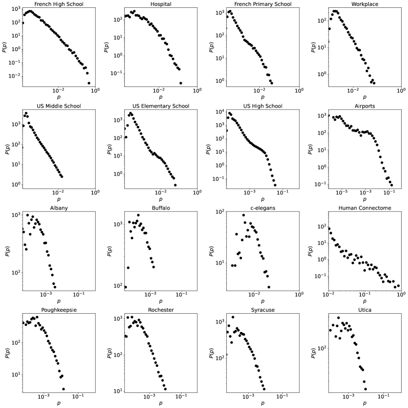
Figure S1: Distribution of proximity values $p$ for the edges in the metric backbone of the empirical networks described in Table S1.

Figure S2: Number of metric edges removed for synthetic networks relative to the size of the sparsified network governed by $\chi$. $\chi$ spans from $\chi=1$, corresponding to not removing any edges, to $\chi=0$ where $E^{sm}$ edges are removed. In the synthetic networks the backbone is fixed as well as the dispersion parameter, $\sigma=1$, of the log-normally distributed semi-metric distortion. The left figure correspond to the setting the log median to $\mu=1$, while on the right we have $\mu=2$.

Figure S3: Ratio between the time for the disease to reach half the population in the sparsified network and in the empirical networks $\xi^{x}_{1/2}$ for each sparsification method $x$ (color code) as a function of the parameter $\chi$, governing the edges removed from the network. $\chi$ spans from $\chi=1$, corresponding to not removing any edges, to $\chi=0$ where $E_{sm}$ edges are removed. Three different sparsification methods are compared: target edges with highest semi-metric distortion values (SmD), lowest effective resistance values (EffRes) or lowest proximity values (W). The details of the simulations to obtain the ratios are the ones described in the main text. EffRes and W curves are interrupted when edges removal breaks the largest connected component of the network (e.g. Poughkeepsie and c-elegans).

Figure S4: Distribution of the relative difference $\tilde{\Delta\xi}^{x}_{y}$ between the times to reach a given fraction $y$ of the population, comparing each sparsification method $x$ (color code) with the one following semi-metric distortion (black dashed line), as a function of the size of the sparsified network $\chi$. $\chi$=1 preserves all the connections in the network whereas $\chi=0$ corresponds to networks whose number of connections matches the size of the metric backbone. Positive $\tilde{\Delta\xi}^{x}_{y}$ values reveal a better performance of the networks sparsified following semi-metric distortion with respect to the other two methods. Dots represent each of the 16 networks included in the dataset under study whereas solid lines show the median $\tilde{\Delta\xi}^{x}_{y}$ value observed across the set of empirical networks. The fraction of the population $y$ used in each panel are: $10\%$ (panel a), $30\%$ (panel b), $70\%$ (panel c) and $90\%$ (panel d).

References

- Keeling and Eames (2005) M. J. Keeling and K. T. Eames, Journal of the royal society interface 2, 295 (2005).
- Morris (2004) M. Morris, Network epidemiology: a handbook for survey design and data collection (OUP Oxford, 2004).
- Metcalf et al. (2020) C. J. E. Metcalf, D. H. Morris, and S. W. Park, Science 369, 368 (2020).
- Pagel and Yates (2022) C. Pagel and C. A. Yates, bmj 378 (2022).
- Blondel et al. (2015) V. D. Blondel, A. Decuyper, and G. Krings, EPJ data science 4, 1 (2015).
- Stehlé et al. (2011) J. Stehlé, N. Voirin, A. Barrat, C. Cattuto, L. Isella, J.-F. Pinton, M. Quaggiotto, W. Van den Broeck, C. Régis, B. Lina, et al., PloS one 6, e23176 (2011).
- Gilbert et al. (2020) M. Gilbert, G. Pullano, F. Pinotti, E. Valdano, C. Poletto, P.-Y. Boëlle, E. d’Ortenzio, Y. Yazdanpanah, S. P. Eholie, M. Altmann, et al., The Lancet 395, 871 (2020).
- Brockmann and Helbing (2013) D. Brockmann and D. Helbing, science 342, 1337 (2013).
- Hazarie et al. (2021) S. Hazarie, D. Soriano-Paños, A. Arenas, J. Gómez-Gardeñes, and G. Ghoshal, Communications Physics 4, 191 (2021).
- Pastor-Satorras and Vespignani (2001) R. Pastor-Satorras and A. Vespignani, Physical review letters 86, 3200 (2001).
- Gómez et al. (2011) S. Gómez, J. Gómez-Gardenes, Y. Moreno, and A. Arenas, Physical Review E 84, 036105 (2011).
- Gómez et al. (2010) S. Gómez, A. Arenas, J. Borge-Holthoefer, S. Meloni, and Y. Moreno, Europhysics Letters 89, 38009 (2010).
- Mata and Ferreira (2013) A. S. Mata and S. C. Ferreira, Europhysics Letters 103, 48003 (2013).
- Silva et al. (2020) D. H. Silva, F. A. Rodrigues, and S. C. Ferreira, Physical Review E 102, 012313 (2020).
- Wang et al. (2017) W. Wang, M. Tang, H. E. Stanley, and L. A. Braunstein, Reports on progress in physics 80, 036603 (2017).
- Shea et al. (2023) K. Shea, R. K. Borchering, W. J. Probert, E. Howerton, T. L. Bogich, S.-L. Li, W. G. van Panhuis, C. Viboud, R. Aguás, A. A. Belov, et al., Proceedings of the National Academy of Sciences 120, e2207537120 (2023).
- Meyers et al. (2003) L. A. Meyers, M. Newman, M. Martin, and S. Schrag, Emerging infectious diseases 9, 204 (2003).
- Della Rossa et al. (2020) F. Della Rossa, D. Salzano, A. Di Meglio, F. De Lellis, M. Coraggio, C. Calabrese, A. Guarino, R. Cardona-Rivera, P. De Lellis, D. Liuzza, et al., Nature communications 11, 5106 (2020).
- Rosenblatt et al. (2020) S. F. Rosenblatt, J. A. Smith, G. R. Gauthier, and L. Hébert-Dufresne, PLoS computational biology 16, e1007897 (2020).
- Mones et al. (2018) E. Mones, A. Stopczynski, A. Pentland, N. Hupert, and S. Lehmann, Journal of The Royal Society Interface 15, 20170783 (2018).
- Wei et al. (2022) X. Wei, J. Zhao, S. Liu, and Y. Wang, Scientific reports 12, 5550 (2022).
- Reyna-Lara et al. (2022) A. Reyna-Lara, D. Soriano-Paños, A. Arenas, and J. Gómez-Gardeñes, Chaos, Solitons & Fractals 158, 112012 (2022).
- Ndeffo Mbah and Gilligan (2011) M. L. Ndeffo Mbah and C. A. Gilligan, PLoS one 6, e24577 (2011).
- Zhu et al. (2021) X. Zhu, Y. Liu, S. Wang, R. Wang, X. Chen, and W. Wang, Applied Mathematics and Computation 411, 126531 (2021).
- Reyna-Lara et al. (2021) A. Reyna-Lara, D. Soriano-Paños, S. Gómez, C. Granell, J. T. Matamalas, B. Steinegger, A. Arenas, and J. Gómez-Gardeñes, Physical Review Research 3, 013163 (2021).
- Bassolas et al. (2022) A. Bassolas, A. Santoro, S. Sousa, S. Rognone, and V. Nicosia, Physical Review Research 4, 023092 (2022).
- Kojaku et al. (2021) S. Kojaku, L. Hébert-Dufresne, E. Mones, S. Lehmann, and Y.-Y. Ahn, Nature physics 17, 652 (2021).
- Ciaperoni et al. (2020) M. Ciaperoni, E. Galimberti, F. Bonchi, C. Cattuto, F. Gullo, and A. Barrat, Scientific reports 10, 1 (2020).
- Wen et al. (2017) S. Wen, J. Jiang, B. Liu, Y. Xiang, and W. Zhou, Journal of Network and Computer applications 78, 288 (2017).
- Chung et al. (2012) N. N. Chung, L. Y. Chew, J. Zhou, and C. H. Lai, Europhysics Letters 98, 58004 (2012).
- Liang et al. (2023) G. Liang, X. Cui, and P. Zhu, Frontiers in Physics 11, 220 (2023).
- Matamalas et al. (2018) J. T. Matamalas, A. Arenas, and S. Gómez, Science advances 4, eaau4212 (2018).
- Serrano et al. (2009) M. Á. Serrano, M. Boguná, and A. Vespignani, Proceedings of the national academy of sciences 106, 6483 (2009).
- Tumminello et al. (2005) M. Tumminello, T. Aste, T. Di Matteo, and R. N. Mantegna, Proceedings of the National Academy of Sciences 102, 10421 (2005).
- Yan et al. (2018) X. Yan, L. G. Jeub, A. Flammini, F. Radicchi, and S. Fortunato, Physical Review E 98, 042304 (2018).
- Radicchi et al. (2011) F. Radicchi, J. J. Ramasco, and S. Fortunato, Physical Review E 83, 046101 (2011).
- Marcaccioli and Livan (2019) R. Marcaccioli and G. Livan, Nature communications 10, 745 (2019).
- Gemmetto et al. (2017) V. Gemmetto, A. Cardillo, and D. Garlaschelli, arXiv preprint arXiv:1706.00230 (2017).
- Imre et al. (2020) M. Imre, J. Tao, Y. Wang, Z. Zhao, Z. Feng, and C. Wang, Computers & Graphics 87, 89 (2020).
- Bravo Hermsdorff and Gunderson (2019) G. Bravo Hermsdorff and L. Gunderson, Advances in Neural Information Processing Systems 32 (2019).
- Spielman and Srivastava (2008) D. A. Spielman and N. Srivastava, in Proceedings of the fortieth annual ACM symposium on Theory of computing (2008), pp. 563–568.
- Simas et al. (2021) T. Simas, R. B. Correia, and L. M. Rocha, Journal of Complex Networks 9, cnab021 (2021).
- Wilson and Kogut (1974) K. G. Wilson and J. Kogut, Physics reports 12, 75 (1974).
- García-Pérez et al. (2018) G. García-Pérez, M. Boguñá, and M. Á. Serrano, Nature Physics 14, 583 (2018).
- Villegas et al. (2023) P. Villegas, T. Gili, G. Caldarelli, and A. Gabrielli, Nature Physics pp. 1–6 (2023).
- Swarup et al. (2016) S. Swarup, S. Ravi, M. H. Mahmud, and K. Lum, Identifying Core Network Structure for Epidemic Simulations (2016).
- Mercier et al. (2022) A. Mercier, S. Scarpino, and C. Moore, PLOS Computational Biology 18, e1010650 (2022).
- Tolić et al. (2018) D. Tolić, K.-K. Kleineberg, and N. Antulov-Fantulin, Scientific reports 8, 6562 (2018).
- Gautreau et al. (2007) A. Gautreau, A. Barrat, and M. Barthélemy, Journal of Statistical Mechanics: Theory and Experiment 2007, L09001 (2007).
- Brattig Correia et al. (2023) R. Brattig Correia, A. Barrat, and L. M. Rocha, PLOS Computational Biology 19, e1010854 (2023).
- Simas and Rocha (2015) T. Simas and L. M. Rocha, Network Science 3, 227 (2015).
- Toth et al. (2015) D. J. Toth, M. Leecaster, W. B. Pettey, A. V. Gundlapalli, H. Gao, J. J. Rainey, A. Uzicanin, and M. H. Samore, Journal of The Royal Society Interface 12, 20150279 (2015).
- Silva and Ferreira (2021) D. H. Silva and S. C. Ferreira, Journal of Physics: Complexity 2, 025011 (2021).
- Cota et al. (2016) W. Cota, S. C. Ferreira, and G. Odor, Physical review E 93, 032322 (2016).
- Estrada et al. (2023) E. Estrada, J. Gómez-Gardeñes, and L. Lacasa, Proceedings of the National Academy of Sciences 120, e2305001120 (2023).
- Lella and Estrada (2020) E. Lella and E. Estrada, Network Neuroscience 4, 1007 (2020).
- Jaccard (1901) P. Jaccard, Bull Soc Vaudoise Sci Nat 37, 241 (1901).
- Hagmann et al. (2008) P. Hagmann, L. Cammoun, X. Gigandet, R. Meuli, C. J. Honey, V. J. Wedeen, and O. Sporns, PLoS biology 6, e159 (2008).
- Watts and Strogatz (1998) D. J. Watts and S. H. Strogatz, nature 393, 440 (1998).