Measuring the Initial-Final Mass-Relation using wide double white dwarf binaries from Gaia DR3

Abstract

The Initial-Final Mass-Relation (IFMR) maps the masses of main sequence stars to their white dwarf descendants. The most common approach to measure the IFMR has been to use white dwarfs in clusters. However, it has been shown that wide double white dwarfs can also be used to measure the IFMR using a Bayesian approach. We have observed a large sample of 90 Gaia double white dwarfs using FORS2 on the VLT. Considering 52 DA+DA, DA+DC, and DC+DC pairs, we applied our extended Bayesian framework to probe the IFMR in exquisite detail. Our monotonic IFMR is well constrained by our observations for initial masses of $1$–$5$ $\mathrm{M}_{\odot}$, with the range $1$–$4$ $\mathrm{M}_{\odot}$ mostly constrained to a precision of $0.03$ $\mathrm{M}_{\odot}$ or better. We add an important extension to the framework, using a Bayesian mixture-model to determine the IFMR robustly in the presence of systems departing from single star evolution. We find a large but uncertain outlier fraction of $59\pm 21$ per cent, with outlier systems requiring an additional $0.70_{-0.22}^{+0.40}$ Gyr uncertainty in their cooling age differences. However, we find that this fraction is dominated by a few systems with massive components near 0.9 $\mathrm{M}_{\odot}$, where we are most sensitive to outliers, but are also able to establish four systems as merger candidates.

1 Introduction

After depleting the hydrogen fuel in their cores, almost all ($\simeq 97$ per cent) main sequences stars end their lives by transitioning to the giant phase and shedding their outer layers in an intense stellar wind. This mass loss that takes place during stellar evolution stops short of the compact central core, which goes on to become a white dwarf. For most white dwarfs, the interior is composed of carbon and oxygen, enveloped by a layer of helium, and finally by a thin but opaque layer of hydrogen at the surface. The most massive white dwarfs, i.e. those with masses $>1.1$ $\mathrm{M}_{\odot}$, will instead have interiors dominated by oxygen and neon (Camisassa et al., 2019). Main sequence stars with masses above about 8 $\mathrm{M}_{\odot}$(Weidemann & Koester, 1983), undergo further nuclear burning during the giant phases, leading to the formation of more exotic stellar remnants via core-collapse supernovae.

It is intuitive to consider that the mass of a main sequence star ought to be correlated with the mass of the resulting white dwarf. More precisely the (final) white dwarf mass can be considered a function of the (initial) main sequence star mass. This function is known as the Initial-Final Mass-Relation (IFMR). The IFMR essentially encodes the amount of mass-loss occurring during stellar evolution for stars of different masses (Bloecker, 1995), and so is an important component for understanding a wide range of astrophysical topics, from stellar evolution itself, to the chemical enrichment of the Galaxy. At a more basic level, the IFMR is also required simply to establish the progenitor masses for studies on individual white dwarfs.

Despite its universal importance, the precise functional form of the IFMR cannot be simply determined. From a computational perspective, determining the IFMR is limited by the predicted mass-loss occurring during the giant branches of stellar evolution, which is extremely sensitive to input physics, such convective and rotational mixing (Marigo & Girardi, 2007; Cummings et al., 2019), and nuclear reaction rates (Fields et al., 2016).

From the observational side, the IFMR can be measured empirically, taking advantage of white dwarf cooling as an accurate clock (Mestel, 1952; Fontaine et al., 2001). Essentially, by accurately measuring the effective temperature ($T_{\mathrm{eff}}$) and mass of a white dwarf, comparison with white dwarf cooling models yields the length of time since the white dwarf left the tip of the Asymptotic Giant Branch (AGB), i.e. the white dwarf cooling age. As long as an independent clock can be sourced to constrain the pre-white dwarf (pre-WD) lifetime, then the initial mass can be determined from stellar evolution models. Thus for a sufficiently large sample of white dwarfs, the relation between initial mass, and final mass can be determined.

The most widely used observational method to determine the IFMR is using white dwarfs in clusters (Weidemann, 1987; Ferrario et al., 2005; Salaris et al., 2009; Williams et al., 2009; Casewell et al., 2009; Dobbie et al., 2009), relying on the fact that the age of a cluster can be measured from the main sequence turn-off. Therefore all white dwarfs within a given cluster (which will have the same total age as the cluster itself), can have their pre-white dwarf lifetimes and hence their initial masses determined empirically. It then becomes a simple matter of fitting some function to the initial-mass/final-mass pairs. The most recent, and most extensive IFMR based on cluster white dwarfs was presented by Cummings et al. (2018), having examined 79 white dwarfs among 13 different clusters, and covering the entire range of initial masses from 0.85 $\mathrm{M}_{\odot}$ to 7.5 $\mathrm{M}_{\odot}$. Even so, such cluster studies are limited by the precision with which initial masses can be determined, and the low number of objects typically found per cluster.

However, cluster white dwarfs are not the only avenue for exploring the IFMR. As an alternative technique, El-Badry et al. (2018) used the population statistics of the Gaia DR2 white dwarf sample, to constrain the IFMR, finding reasonable agreement with results from cluster studies. Catalán et al. (2008) established a different technique to infer the IFMR, examining white dwarfs in common-proper motion pairs (i.e. wide binaries) with main sequence stars. Both components of the system can be assumed to have formed at the same time, but evolving independently due to their wide separation. Specifically when the more massive primary undergoes stellar evolution, no common envelope occurs, and therefore there is no mass transfer onto the secondary. As with clusters the final masses are determined from spectral modelling of the white dwarf, with initial masses estimated by age-dating the main sequence companions using high-resolution spectroscopy. More recently Barrientos & Chanamé (2021) applied a similar technique to 11 white dwarfs with turnoff/subgiant companions whose ages can be determined more precisely than for main sequence companions. While accurate initial masses can be obtained this way, very few white dwarfs are found in binaries with companions at this specific evolutionary stage.

Also employing wide binaries, Andrews et al. (2015) prototyped a new technique for constraining the IFMR, instead using double white dwarfs (DWDs). Once again, both components of the binary are assumed to have evolved separately. However, unlike in the previous examples, one cannot directly infer the pre-WD lifetimes or total ages. Nevertheless, the cooling ages of the two white dwarfs still provide two independent clocks, where their difference ($\Delta\tau_{\mathrm{WD}}$) should have the same magnitude but opposite sign as the difference in pre-white dwarf lifetimes ($\Delta\tau_{\mathrm{preWD}}$), i.e. $\mbox{$\Delta\tau_{\mathrm{WD}}$}=-\mbox{$\Delta\tau_{\mathrm{preWD}}$}$. This can be used to limit the combination of initial masses that can have produced that binary. By modelling DWDs within a Bayesian framework, Andrews et al. (2015) were able to construct a posterior distribution for the IFMR given a set of 19 DWD pairs. This work predates the release of Gaia DR2, with the authors acknowledging the impending deluge of Gaia data would open the opportunity for a much higher fidelity IFMR to be determined.

In this work we adopt and extend the DWD Bayesian approach, first introduced by Andrews et al. (2015) for fitting the IFMR. In Section 2, we introduce our spectroscopically observed DWD sample. In Section 3, we discuss our approach to spectral modelling combined with precise Gaia photometry and astrometry. In Section 4, we explain the Bayesian framework we have adopted to model the IFMR, as well as our extensions to the framework first introduced by Andrews et al. (2015). We show and discuss our resulting IFMR fits in Section 5, testing a variety of assumptions and comparing with other established results from different methodologies. Finally we give our conclusions and areas for future work in Section 6.

2 Double white dwarf sample

2.1 Sample Selection

Our goal was to create as large a possible sample of DWDs. To achieve this, we selected double white dwarfs from Gaia DR2 (Lindegren et al., 2018) by combining the catalogue of El-Badry & Rix (2018) with our own selection. We selected all pairs from the WD catalogue of Gentile Fusillo et al. (2019) with parallaxes and proper motions consistent within 3$\sigma$. We limited our sample to those DWDs with accurate parallaxes ($\pi/\sigma_{\pi}>10$) and projected separations of less than 10 000 au. We also required small errors on proper motion, $\sqrt{\sigma^{2}_{\rm pm\_ra}+\sigma^{2}_{\rm pm\_dec}}<6$ mas. Our chosen selection was designed to supplement El-Badry & Rix (2018) with DWDs at larger distances, and those that have poor quality photometry in Gaia DR2.

Our selection includes 424 DWDs, whilst the catalogue of El-Badry & Rix (2018) contains 375. There is only moderate overlap between the two samples, with 214 DWDs being common to both: 161 objects are found in El-Badry & Rix (2018), but not in our sample. The majority of these (120) are close systems which pass the looser parallax and proper motion cuts of El-Badry & Rix (2018), that are designed to accommodate orbital motion of the DWD. A further 27 are explained by the relaxed separation constraint (50 000 vs 10 000 AU) of El-Badry & Rix (2018), and 14 are missing from our selection for unknown reasons. Our selection includes 210 DWDs which are not reported by El-Badry & Rix (2018). The vast majority of these are either beyond 200 pc, or do not pass the cuts placed on the quality of photometry in El-Badry & Rix (2018). Of those 210, 23 systems are missing from El-Badry & Rix (2018) for unknown reasons.

Our final sample consists of 585 high-confidence DWDs, albeit with a complex set of selection criteria. With the improved astrometry of Gaia DR3 (Gaia Collaboration et al., 2021), 99.8 percent remain in our sample, and none of the rejected objects were observed.

2.2 Observations

From our sample of 585 DWDs, we observed 90 systems with the European Southern Observatory (ESO) Very Large Telescope (VLT) Focal Reducer and Low Dispersion Spectrograph (FORS2) under programs 103.D-0718 and 109.213B. A summary journal of observations is provided in Table 1. Runs A, B and C were observed under program 103.D-0718 on the nights of June 1 2019, July 2–3 2019, Sep 24 2019 respectively. Runs D and E were observed under program 109.231B on the nights of June 2–3 2022 and 21 Sep 2022 respectively.

For runs A, B and C targets were selected based on brightness and visibility. Objects with existing Sloan Digital Sky Survey (SDSS) spectra were not observed and we preferentially chose systems with large cooling age and mass differences, based on the values provided in Gentile Fusillo et al. (2019). Prompted by the large fraction of magnetic white dwarfs amongst the systems observed in these runs (see Section 2.3 for details), for runs D and E we simply selected targets at random from the visible DWD systems without SDSS spectra. A Hertzsprung-Russel diagram of the observed systems is shown in Figure 1, with Gaia astrometry/photometry and spectral classifications given in Table LABEL:tab:dwds_obs.

All observations were taken using the 1200B+97 grating with a 0.7 ″ slit, giving a wavelength range of 3660–5010 Å at a resolution of $R=2000$. The slit was oriented to place both white dwarfs on the slit simultaneously. The data were reduced using the esoreflex FORS2 pipeline v5.6.2 and standard procedures. Spectra were extracted using optimal extraction (Horne, 1986) and a modification of the pipeline was made to prevent the extraction window of faint targets being reduced if a brighter target is nearby on the CCD. Wavelength calibration was performed using a combination of arc lamp images and the location of bright sky lines.

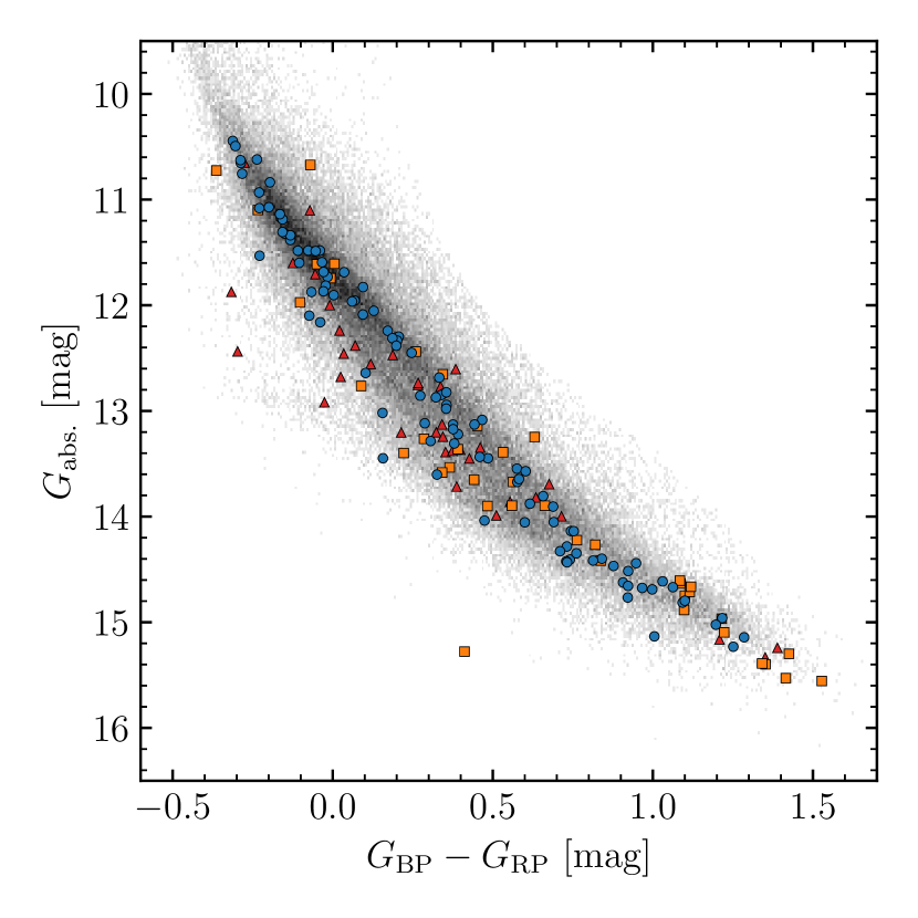
Figure 1: Gaia DR3 Hertzsprung-Russel diagram of our DWD sample observed with FORS2. Red triangles are white dwarfs that were deemed unsuitable for spectroscopic fitting with DA models (e.g. due to that component or its companion having exhibiting strong magnetism or an unambiguous helium atmosphere). Orange squares are white dwarfs with spectroscopic fits, but were not used to fit the IFMR (e.g. due to that component or its companion having an extremely low mass or otherwise poor spectroscopic fit; see Section 3.3.1). The remaining white dwarfs (blue circles) were deemed suitable to constrain the IFMR (Section 5). The grey-scale background uses data from Gentile Fusillo et al. (2021).

Table 1: Observing log for the different nights of observation. $N_{\mathrm{obs}}$ is the number of systems observed in each run.

Run	MJD	$N_{\mathrm{obs}}$
A	58 634–58 635	24
B	58 666–58 667	13
C	58 750	23
D	59 732–59 733	18
E	59 843	14

2.3 Systems rejected from fitting

Out of our 90 observed systems, there were 18 systems we chose not to fit at all as we did not believe we could derive meaningful atmospheric parameters (red triangles in Figure 1). For $12$ of these, this was because at least one component exhibited a strong magnetic field. These systems are WD J0059$-$2417AB, WD J0220$-$1532AB, WD J0224$-$4611AB, WD J0344$+$1509AB, WD J0902$-$3540AB, WD J1159$-$4630AB, WD J1834$-$6108AB, WD J2018$+$2129AB, WD J2023$-$1446AB WD J2047$-$8206AB, WD J2304$-$0701AB, and WD J2353$-$3620AB. Note that while WD J2023$-$1446AB contains a strongly magnetic DA, it is primarily excluded from fitting due to its baffling A component (Section 2.4). Furthermore, four spectra exhibited an unambiguous helium-dominated atmosphere (either due to helium lines or pressure broadened metal lines). These systems are WD J0225$-$1756AB, WD J1813$+$0604AB, WD J1836$-$5114AB, and WD J2355$+$1708AB. Finally two systems, WD J1310$-$3930AB and WD J2115$+$2534AB, contained white dwarfs with blue DC spectra which could plausibly be explained by either strong magnetism or helium dominated atmospheres. In total this left 72 systems used to perform spectroscopic fits.

2.4 Notes on individual systems

WD J1953$-$1019AB
This system is part of a resolved triple white dwarf, first reported by Perpinyà-Vallès et al. (2019). Our observations refer to the A and C components from the discovery paper. In hindsight, it would have been ideal to observe all three components of this system to provide further constraints on the IFMR. That said, Perpinyà-Vallès et al. (2019) found that the B and C components (the inner binary) have almost identical atmospheric parameters. The potential for this system to provide a strong constraint on the IFMR is therefore limited compared to an idealised case where all three components have substantially different masses and cooling ages.

WD J2023$-$1446AB
While we are unable to use this system for fitting the IFMR, both components of this wide binary are noteworthy. The B component has a spectral type DAH. The H$\beta$ absorption line shows Zeeman splitting indicative of a $14$ MG magnetic field. The A component, however, is extremely unusual and while resembling a hot DQB, an assignment of DX (Sion et al., 1983) is more accurate: Its position in the Gaia HR diagram indicates a mass of $\simeq 1.2$ $\mathrm{M}_{\odot}$ (Gentile Fusillo et al., 2021), and a plethora of lines are apparent in the spectrum (Figure 2), none of which we have been conclusively able to assign. While a strong magnetic field with a non-hydrogen atmospheric composition provides a plausible explanation for these observations, if we allow for a large blue-shift of 1050 km s^-1 (not accounting for the presumably substantial gravitational redshift), some of the strongest lines can be assigned to C ii, and a few to He i (Figure 2), with no evidence of Zeeman splitting observed. Nevertheless, around one third of the spectral features remain unassigned, and some predicted spectral lines are absent. While the proposed blue-shift could be explained as a wavelength calibration issue, we found no evidence for this, and the A component shows no similar shift, despite being observed simultaneously. Furthermore, we obtained a second set of observations of this system in our third FORS2 run (run C), finding a similar spectrum with features occurring at the same wavelengths, though many with different strengths.

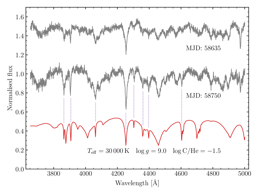
Figure 2: Normalised spectra of WD J2023$-$1446A (grey) with a DQB model shown in red. The spectra and model are offset by 0.5 from one another. The model has been blue shifted by 1050 km s^-1 with identified C ii lines indicated by the dotted purple lines.

Both components have similar proper-motions of about $17$ mas yr^-1, implying a $v_{\perp}$ of 15 km s^-1 for the system. Crucially, the difference in $v_{\perp}$ is $<1.7$ km s^-1 at the 99th percentile, which at an on-sky separation of 2000 au rules out the possibility of a chance alignment. Given the somewhat convincing velocity shift, it is tempting suggest WD J2023$-$1446A may itself be part of a close binary with a hidden companion, where both epochs were by chance observed at the same extremum in orbital velocity. While a much cooler white dwarf could remain hidden by the flux of WD J2023$-$1446A, the short orbital period (required for an orbital velocity $>1050$ km s^-1) would lead to orbital smearing of the spectra. An orbital period of a few 10 hr could instead be achieved with a stellar-mass black hole companion, but such a scenario is obviously contrived. Light curves we have obtained of this object show no variability above the 1 percent level. As it has no bearing on our investigation of the IFMR, we refrain from speculating further on the nature of this peculiar system.

WD J1336$-$1620AB
This system was first observed during observing run A, and subsequently re-observed during run D. While unintentional, it provided the opportunity to determine the level of systematic uncertainty in our spectroscopic fits. With essentially four observations (two per binary component), we were able to constrain the $T_{\mathrm{eff}}$ relative precision to $0.9_{-0.4}^{+1.0}$ percent, and the $\log g$ precision to $0.043_{-0.017}^{+0.045}$ dex. These precisions can be used as priors in Section 4.3.

WD J2018$+$2129AB
This system appears to be a rare wide binary where both components are magnetic. In the A component, Zeeman splitting of the Balmer lines is observed, indicative of a $\simeq 1$ MG field. At a glance, the B component spectrum resembles a DC spectral type, though closer inspection reveals broad wavy absorption bands characteristic of a strongly magnetic atmosphere with a field strength in the 100s of MG (see WD J1159$-$4630B, WD J1834$-$6108A WD J2047$-$8206A, WD J2304$-$0701A, or WD J2353$-$3620B for more obvious examples). To our knowledge this is the only known wide DWD where both components exhibit magnetism.

3 Spectral modelling

3.1 DA model grid

To obtain atmospheric parameters for our double white dwarf sample, we calculated a two-dimensional grid of pure hydrogen model spectra using the Koester white dwarf model atmosphere code (Koester, 2010, 2013). Effective temperatures ($T_{\mathrm{eff}}$) were calculated from 3500 K to 10 000 K in steps of 250 K, then up to 20 000 K in steps of 500 K, and finally up to 35 000K in 1000 K steps. The grid was evaluated for surface gravities ($\log g$) from 7.00 to 9.50 in 0.25 dex steps (cgs units). All models were calculated with a convective mixing length parameter $\mathrm{ML2}/\alpha$ (Tassoul et al., 1990) of $0.8$. This choice of 0.8 allows easy application of 3D corrections to our spectroscopic parameters (see below).

Each model spectrum was convolved to an instrumental resolution of 1.8 Å, as appropriate for our FORS2 grating and slit-width combination. For each combination of $T_{\mathrm{eff}}$ and $\log g$, we determined the stellar radius, $R_{\mathrm{WD}}$, using the mass-radius relation from Bédard et al. (2020) appropriate for white dwarfs with thick hydrogen layers. Since the Koester model fluxes are in units of $4\times$ Eddington-flux, we scaled each model in the grid by a factor $\pi(R_{\mathrm{WD}}/1\,\mathrm{kpc})^{2}$. As an additional step we applied gravitational redshifts to each model in our grid, using same mass-radius relation as before. In principle this allows our fits to be sensitive to the difference in gravitational redshift for the two components of a binary (assuming negligible orbital reflex motion), with the systemic radial velocity necessarily included as an additional free parameter.

To generate fluxes for arbitrary $T_{\mathrm{eff}}$ and $\log g$ and wavelength, we used tri-linear interpolation of the logarithm of the model grid fluxes. The use of the log-fluxes is necessary as wavelengths bluer than the peak have a strongly non-linear dependence on $T_{\mathrm{eff}}$.

Since these models are 1-dimensional, they require correction to the corresponding 3D parameters for the most physically accurate results. We adopted the corrections given by Tremblay et al. (2013), applying their Equations (9) and (10), appropriate for the ML2/$\alpha=0.8$ used in our model atmosphere calculations.

3.2 Spectrophotometric fitting

To fit each DWD, we used not only the FORS2 spectra, but also the Gaia DR3 photometry to constrain the atmospheric parameters. We first fit each binary using a least squares approach, following this up with a Markov-Chain Monte-Carlo analysis for more informative parameter distributions.

Inspecting the FORS2 spectra, it was clear that the flux calibrations were generally poor, though in a consistent manner for each DWD, i.e. unphysical curvature in the spectral continuum of the A component would also be observed in the spectrum of the B component (as a result of both stars being observed on the slit simultaneously). We therefore took advantage of these shared systematic uncertainties by fitting both components of the binary simultaneously. Specifically, we modelled the wavelength dependent flux calibration correction as a 5th-order polynomial. While we found this approach to be generally successful, we found that the relative fluxes can differ by a constant factor, e.g. if one component was slightly off-centre on the slit compared to the other. We therefore introduced a further free-parameter to re-scale the fluxes of the B-component by a constant amount. A demonstration of our approach to flux calibrations is shown in Figure 3 for the system WD J0023$+$0643AB.

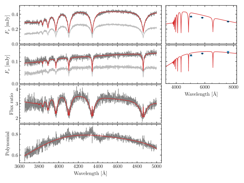
Figure 3: Best fit to WD J0023$+$0643AB. The A and B components are shown in the top two rows. The left columns show the spectra with their original flux calibrations (light grey), compared with re-calibrated spectra (medium grey), and the best fitting models (red). The right columns show the Gaia DR3 fluxes (blue points with error bars), against the model synthetic photometry (black points) – note that the spectral models are shown for illustrative purposes only, and do not overlap the synthetic points due to the broadness of the Gaia bandpasses. The second bottom panel shows the ratio of fluxes compared with the ratio of model spectra, demonstrating excellent agreement in the wings and line cores. The bottom panel shows the ratio of original spectra to their best fitting models (averaged over the A and B components) against the flux-correcting 5-th order polynomial.

Initially, we performed a least squares fit to the spectra and Gaia photometry to constrain the flux correcting polynomial, the flux scaling factor on the B-component, the $T_{\mathrm{eff}}$ and $\log g$ for each component, and the systemic radial velocity. Furthermore, we included the parallax as a free-parameter in order to marginalise over the uncertainty of the Gaia measurement. We then used the best fitting parameters and covariance matrix to initialise a Markov-Chain Monte-Carlo fit via the python package emcee (Foreman-Mackey et al., 2013).

As part of the MCMC we introduced two new free parameters. In a few cases, where one white dwarf is significantly brighter than its companion, the bright component may have an extremely high S/N ratio (in order to get sufficient counts for the fainter component). This may cause that spectrum to dominate the fit entirely. To avoid this, we introduced a relative noise floor parameter, $\eta$ to our fits. Simply put, we increased the flux uncertainties according to $\sigma_{i}^{\prime 2}=\sigma_{i}^{2}+(\eta\times f_{i})^{2}$, where $\sigma_{i}^{\prime}$ and $\sigma_{i}$ are the modified and modified flux uncertainties, and the $f_{i}$ are the spectroscopic fluxes at wavelength $i$. Compared with the usual $-\tfrac{1}{2}\chi^{2}$, the addition of this noise-floor requires a slightly modified log-likelihood for each spectrum,

$$\ln L=-\tfrac{1}{2}\chi^{2}-\sum_{i}^{N}\ln\sigma_{i}^{\prime},$$ (1)

where $\chi^{2}$ has the usual meaning and implicitly depends on the $\sigma_{i}^{\prime}$. A uniform prior for $\eta>0$ was used on this parameter. Similarly we folded in a 1 percent additional flux to the Gaia fluxes according to the Gaia documentation on the uncertainty on the absolute calibration scales.

Our sample of DWDs have Gaia parallaxes locating them at distances up to 250 pc, with a median of 90 pc. Therefore it is reasonable to assume that the Gaia fluxes for some of the more distant objects will be affected by interstellar reddening. Indeed in our initial attempts at fits (which did not include reddening), we found some cases where a good fit to the spectra resulted in models that were bluer than the Gaia photometry, affecting primarily the more distant objects such as WD J1336$-$1620AB. To account for this we included interstellar reddening, specifically $E(B-V)$, as a an additional free parameter. For the MCMC fits, we used the Jeffreys prior, $P(E(B-V))\propto E(B-V)^{-1/2}$, which is naturally weighted towards lower values on a linear scale, but is also a proper prior as long as an upper-bound is provided. For each DWD, we queried the Bayestar19 3D extinction maps (Green et al., 2019) to determine the 99th percentile of $E(B-V)$ at the specified distance of the system. This was then used as upper-bound on our reddening prior. For systems outside of the Bayestar footprint, we adopted $E(B-V)=10^{-4}$ as the upper limit if located within 100 pc of the Sun, or $0.15$ otherwise. For the most nearby systems, where the queried 99th percentile may return exactly zero, we also set the upper-limit at $10^{-4}$ for numerical stability.

For the priors on the remaining free parameters we used normal distributions on both $\log g$s of $\mathcal{N}(\log g;8.0,0.25)$ (units of dex) to approximate the white dwarf mass distribution in the absence of any other strongly constraining data, though in practice, even in the worst case we found the data constrained the $\log g$ to within $\pm 0.11$ dex. For the radial velocity $r$, we again used a normal distribution $\mathcal{N}(r;0,200)$ (units of km s^-1) specifically to avoid $r$ becoming unbounded when fitting DC+DC pairs. Finally, for the two $T_{\mathrm{eff}}$, we used flat priors on a logarithmic scale to reflect the greater abundance of cool white dwarfs in volume limited samples compared to the hottest objects.

3.3 Spectroscopic results

For the MCMC fits themselves, for each system, we used an ensemble of 200 walkers. We found that most of these had fully burnt-in within about 2000 steps. Therefore we chose to run for 5000 steps, using the final 1000 steps (thinned to every 5 steps) to report the final results. The best parameters for all 72 fitted binaries are shown in Table LABEL:tab:dwds_fits, including derived parameters (masses, cooling ages, and difference in cooling ages). Spectra, photometry and best fitting hydrogen atmosphere models for all systems are shown in Figures LABEL:fig:fits01–LABEL:fig:fits31. These figures include systems that we did not fit (Section 3.3.1), but which are shown without models.

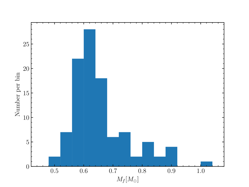
Figure 4: Mass distribution of our 104 white dwarfs (52 binary systems) used to fit the IFMR.

The white dwarf mass distribution of all objects used to perform IFMR fitting is shown in Figure 4 (details of additional excluded systems are given in Section 3.3.1). These white dwarfs have a median mass of 0.626 $\mathrm{M}_{\odot}$, with the distribution appearing broadly similar to white dwarf mass distributions from other works (Genest-Beaulieu & Bergeron, 2014; Rebassa-Mansergas et al., 2015; Hollands et al., 2018).

3.3.1 Systems excluded for fitting the IFMR

The vast majority of our fits are consistent with both spectroscopy and photometry (Figures LABEL:fig:fits01–LABEL:fig:fits24), therefore giving us confidence that they are suitable to fit the IFMR. Even so, there are some systems where, for one reason or another, we do not trust our atmospheric parameters, and so exclude them from the following parts of this work.

Four systems contain magnetic white dwarfs with field strengths of a few MG. Due to Zeeman splitting, the resulting fits had synthetic photometry that were entirely inconsistent with the Gaia data. These systems are WD J0002$+$0733AB, WD J0240$-$3248AB, WD J1314$+$1732AB, WD J1636$+$0927AB, and WD J2259$+$1404AB. Note that WD J1535$+$2125B exhibits a weak $<1MG$ magnetic field, which does not appear to have affected the quality of its spectroscopic fit. Therefore we see no reason to reject this system.

Many systems contain one or more DC white dwarfs. Some of these remain ambiguous as to whether they could have hydrogen or helium dominated atmospheres. However a few systems, show severe disagreement with their best fitting hydrogen-dominated model spectra. The white dwarfs in question are WD J1124$-$1234A, WD J1350$-$5025A, WD J1729$+$2916B, WD J1929$-$3000B, and WD J2122$+$3005A. In most of these cases the fit attempts to reduce the strength of the hydrogen lines by reducing the $T_{\mathrm{eff}}$, resulting in extremely poor agreement with the photometry. Regardless, these systems have been fitted with an incorrect atmospheric model, and so must be rejected.

As stated above, some systems containing one or more DCs remain ambiguous. These are generally DCs with $\mbox{$T_{\mathrm{eff}}$}<5000$ K, which would not show strong hydrogen lines regardless of their atmospheric composition. Therefore we rely on the photometry to assess the quality of the fits. Indeed, some DA+DC systems such as WD J0109$-$1042AB show excellent agreement with the photometry of the DC component, suggesting that object does indeed have a hydrogen dominated atmosphere. However, WD J0007$-$1605A, WD J1827$+$0403A, and WD J1859$-$5529B show disagreement suggesting they instead likely have helium dominated atmospheres. We therefore exclude these three systems.

Our sample also contains DC+DC pairs introducing further ambiguity, as the atmospheric parameters for both components are essentially determined only by the photometry. All of these DC+DC systems, e.g. WD J0104$+$2120AB, show good agreement with their photometry. However, we found that several of these DC+DC pairs contained one or more white dwarfs with low derived masses implying they cannot have formed via standard evolution, as the universe is not old enough to have produced such low mass objects assuming single star evolution for both components. Therefore such systems must be rejected on the basis that they cannot constrain the IFMR. These systems are WD J1014$+$0305AB, WD J1211$-$4551AB, WD J1557$-$3832AB, WD J1804$-$6617AB, WD J1827$+$0403AB, WD J1929$-$4313AB, WD J2122$+$3005AB, WD J2230$-$7513AB, and WD J2248$-$5830AB.

After rejecting these 20 problematic systems (WD J1827$+$0403AB and WD J2122$+$3005AB are rejected on account of multiple reasons), our final sample we used to fit the IFMR contained 52 systems (mass distribution shown in Figure 4).

3.3.2 Comparison of results

Since all objects in our sample were drawn from the DR2 catalogue of Gentile Fusillo et al. (2019) and subsequently are present in the EDR3 catalogue of Gentile Fusillo et al. (2021), we sought to compare our combined spectroscopic+photometric fits with the photometric results of Gentile Fusillo et al. (2021). In Figure 5, we show the difference between these sets of results for both $T_{\mathrm{eff}}$ and $\log g$, though specifically for the 52 binaries (104 white dwarfs) selected to constrain the IFMR. In both panels, the uncertainties in $T_{\mathrm{eff}}$/$\log g$ differences are generally dominated by the contribution from the Gentile Fusillo et al. (2021) results, since we use the same photometric data for our fits, but have the benefit of spectroscopy.

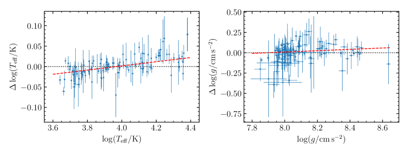
Figure 5: Comparison between our combined spectroscopic+photometric fits, and the photometric fits of Gentile Fusillo et al. (2021). This includes only the 52 systems (104 white dwarfs) used to constrain the IFMR, i.e. systems with poor fits due to magnetism or helium dominated atmospheres or extremely low masses are not shown. The dashed red lines indicate linear fits to the $\log\mbox{$T_{\mathrm{eff}}$}$ and $\log g$ differences.

In the left panel, a small but statistically significant linear trend is seen in the difference in results as a function of temperature. Specifically, we find a gradient of $0.051\pm 0.007$, or equivalently $11.8\pm 1.5$ percent dex^-1. Across the range of data, this means we find 4 percent lower $T_{\mathrm{eff}}$ at $\log(\mbox{$T_{\mathrm{eff}}$}/\mathrm{K})=3.65$ ($\simeq 4500$ K), consistent results at 9300 K, and 5 percent higher $T_{\mathrm{eff}}$ at $\log(\mbox{$T_{\mathrm{eff}}$}/\mathrm{K})=4.4$ ($\simeq 25\,000$ K). The results for the surface gravities are much more consistent, with the best fitting linear trend only varying by about 0.005 dex across the observed range of data (Figure 5).

The $T_{\mathrm{eff}}$ differences, while generally small are still worth investigating as small changes in $T_{\mathrm{eff}}$ will result in larger differences in cooling ages. The source of this discrepancy could result from differences in the model atmospheres used between our work (Koester models) and the work of Gentile Fusillo et al. (2021) (Tremblay models), the fact that we used spectroscopy and photometry rather than just photometry, or fitting methodology. As a test we tried fitting the Gaia photometry alone. In this case, the linear trend in $T_{\mathrm{eff}}$ differences disappeared, suggesting the addition of spectroscopy is responsible. We note that despite finding no linear trends, our photometric fits were on average 3 percent lower in $T_{\mathrm{eff}}$ compensated by results 0.04 dex lower in $\log g$, indicating some remaining difference between atmosphere models or fitting methodology.

Differences in spectroscopic and photometric stellar parameters are well documented (Bergeron et al., 2019). Despite these differences we note that given the size of the error-bars, we are still generally within 1–2$\sigma$ of the results from Gentile Fusillo et al. (2021). Given that our spectroscopy provides significantly more data with which to work with, it is likely that our results are more accurate. Even so, in Section 4.2, we demonstrate the ability of our IFMR model to account for systematic uncertainty in $T_{\mathrm{eff}}$ and $\log g$ parameters, and so this is not expected to affect our results on fitting the IFMR.

4 Modelling the IFMR

In this section, we explain our Bayesian model for investigating the IFMR using wide DWDs. This is essentially an adaptation of the framework first introduced by Andrews et al. (2015), though presented in a mathematically simplified way. Furthermore, we have expanded the framework, accounting for correlated and underestimated $T_{\mathrm{eff}}$ and $\log g$ uncertainties, as well as allowing for the possibility that some fraction of systems are outliers that violate the assumption of coeval stellar evolution. Our implementation of this model will be made available at https://github.com/mahollands/IFMR_DWDs.

4.1 Bayesian framework

Given a set of observed wide DWDs with measured parameters, we ultimately wish to determine the distribution of IFMRs consistent with our data. In Bayesian notation this means our desired posterior distribution can be written as

$$P(\mathrm{IFMR}|\mathrm{DWDs})\propto P(\mathrm{IFMR})\times P(\mathrm{DWDs}|\mathrm{IFMR}),$$ (2)

where the terms on the right are the prior probability distribution on the IFMR, and the likelihood of obtaining our data given a specific IFMR, respectively. Since each of the DWDs represent independent observations, the likelihood in Equation (2) can be written as a product of likelihoods for each double white dwarf (DWD_k),

$$P(\mathrm{DWDs}|\mathrm{IFMR})=\prod_{k}^{N}P(\mathrm{DWD}_{k}|\mathrm{IFMR}).$$ (3)

More explicitly, the relevant measured observables for each DWD are the two white dwarf (final) masses ($M_{f1}$ and $M_{f2}$) and the difference in their white dwarf cooling ages, $\Delta\tau_{\mathrm{WD}}$. Furthermore these parameters have measurement uncertainties, which we encapsulate in a covariance matrix, $\Sigma$. Written out explicitly, the individual DWD likelihood in Equation (3) can be written as

$$P(\mathrm{DWD}|\mathrm{IFMR})=P(M_{f1},M_{f2},\mbox{$\Delta\tau_{\mathrm{WD}}$}|\mathrm{IFMR},\Sigma),$$ (4)

where we have dropped the index, as the DWD in question is no longer explicitly from a larger set of DWDs. All that remains is to determine the functional form of this likelihood, though how to do so is not immediately obvious.

If instead we had prior knowledge of the initial masses, $M_{i1}$ and $M_{i2}$, things become much clearer. The predicted final masses could then be determined directly from the initial masses and IFMR. The difference in cooling ages could also be predicted from the main sequence lifetimes corresponding to these initial masses, recalling that $\mbox{$\Delta\tau_{\mathrm{WD}}$}=-\mbox{$\Delta\tau_{\mathrm{preWD}}$}$ for coeval systems. Mathematically the likelihood for a DWD with a given IFMR and given initial masses can be written as

$$P(\mathrm{DWD}|\mathrm{IFMR},M_{i1},M_{i2})=\frac{1}{\sqrt{(2\pi)^{3}|\Sigma|}}\exp\left(-\tfrac{1}{2}\mathbf{X}^{T}\Sigma^{-1}\mathbf{X}\right),$$ (5)

where $\mathbf{X}$ is defined as

$$\mathbf{X}=\left(\begin{array}[]{c}M_{f1}-\mathrm{IFMR}(M_{i1})\\ M_{f2}-\mathrm{IFMR}(M_{i2})\\ \mbox{$\Delta\tau_{\mathrm{WD}}$}+\mbox{$\Delta\tau_{\mathrm{preWD}}$}(M_{i1},M_{i2})\\ \end{array}\right),$$ (6)

In principle this likelihood could be used directly to determine the IFMR, by constructing a posterior distribution where the initial masses per system are also free parameters to be sampled. In practice however, for large sets of DWDs such as ours, the posterior distribution becomes too highly dimensional to sample in finite time.

To ensure that the posterior distribution has as few free-parameters as possible (i.e. the parameters defining the IFMR), we can instead marginalise over the initial masses by integrating over them, i.e.

$$P(\mathrm{DWD}|\mathrm{IFMR})=\iint P(\mathrm{DWD}|\mathrm{IFMR},M_{i1},M_{i2})\,\mathrm{d}M_{i1}\,\mathrm{d}M_{i2},$$ (7)

recovering the desired likelihood in Equation (4). Conceptually, the process of integration takes into account all possible combinations of $M_{i1}$ and $M_{i2}$ leading to a likelihood where the distribution of data depends only on the IFMR. Even more rigorously, the integrand in Equation (7) can be multiplied by a prior-distribution on $M_{i1}$ and $M_{i2}$ to weight the distribution by initial masses that are more common, i.e. an initial mass function (IMF) as a prior. In our implementation we use a Salpeter IMF (Salpeter, 1955) with exponent $\alpha=2.3$, i.e. the high mass part of the Kroupa IMF (Kroupa, 2001), and apply this to both components.

In practice this integration step must be performed numerically, presenting its own set of challenges. The integral must be calculated many times (specifically the number of times the likelihood in Equation (3) is evaluated multiplied by the number of DWDs in the sample), therefore computationally expensive integration techniques such as Gaussian quadrature are not appropriate here. Furthermore, for some specific DWD and IFMR sample, only a small region of the $M_{i1}$-$M_{i2}$ plane will contribute any significant probability density, making the choice of integration limits difficult (in order to avoid integrating over regions of near-zero probability density).

The joint-distribution of final masses, however, is known, and so for any given IFMR, the corresponding region in the $M_{i1}$-$M_{i2}$ plane can be determined, subject to the condition that the IFMR is monotonic (and thus invertible). Therefore by performing a change of variables, we can instead perform the integration in the $M_{f1}$-$M_{f2}$ plane, transforming the integral in Equation (7) into

$$\iint P(\mathrm{DWD}|\mathrm{IFMR},M_{i1},M_{i2})\frac{\partial M_{i1}}{\partial M_{f1}}\frac{\partial M_{i2}}{\partial M_{f2}}\,\mathrm{d}M_{f1}\,\mathrm{d}M_{f2},$$ (8)

where the Jacobian terms are simply the gradient of the inverse IFMR evaluated at $M_{f1}$ and $M_{f2}$, and the $M_{i}$ are determined by plugging the $M_{f}$ into the inverse IFMR. Since the joint distribution of $M_{f1}$ and $M_{f2}$ has already been measured from the data, we can use Monte-Carlo samples from this distribution, restricting ourselves to a small area in the $M_{f1}$-$M_{f2}$ plane (and the equivalent area in the $M_{i1}$-$M_{i2}$ plane) to perform the integral in Equation (8).

We achieve this numerical approach using the technique of importance sampling. In importance sampling, one can evaluate the integral of a function $f(\mathbf{x})$ (where $f$ may be multivariate) by drawing $N$ samples, $\mathbf{x}_{i}$, from a distribution $P(\mathbf{x}$). The integral may then be approximated as

$$\int f(\mathbf{x})\,\mathrm{d}\mathbf{x}\approx\frac{1}{N}\sum_{i}^{N}\frac{f(\mathbf{x}_{i})}{P(\mathbf{x}_{i})}.$$ (9)

Therefore importance sampling essentially turns the integral into a weighted mean, where – assuming that $P(\mathbf{x})$ has been chosen to be similar in shape to $f(\mathbf{x})$ – the density of samples is highest close to where $f(\mathbf{x})$ is maximised, and few samples are placed at values of $\mathbf{x}$ that contribute little to the integral of $f$. Thus, the sample weights are simply $1/P(\mathbf{x}_{i})$, and where $P$ is normalised over the space $\mathbf{x}$.

In our case, we draw samples of $M_{f1}$ and $M_{f2}$ from a multivariate-normal distribution using the mean and covariance matrix derived from our spectroscopic fits, which can then be used to evaluate the double integral in Equation (8). We demonstrate this approach in Figure 6, where we use a 3-segment mock-IFMR to calculate the likelihood for WD J2007$-$3701AB in the $M_{f1}$-$M_{f2}$ plane. The red points represent 300 random draws from the measured values of $M_{f1}$ and $M_{f2}$, and their covariance matrix. The likelihood is slightly narrower than the distribution of Monte-Carlo samples, as it is further constrained by the measurement of $\Delta\tau_{\mathrm{WD}}$. Although this means some of the 300 samples have very low likelihood, evaluating Equation (7) directly would require sampling the entire $M_{i1}$-$M_{i2}$ plane, with almost all samples close to zero likelihood. We reiterate that integration over the $M_{f1}$-$M_{f2}$ plane via importance sampling, while drastically improving the computational efficiency of calculating the likelihood, explicitly depends on the IFMR model being monotonic – an assumption for which some recent works suggest may not be justified (see Sections 5.4 and 5.5).

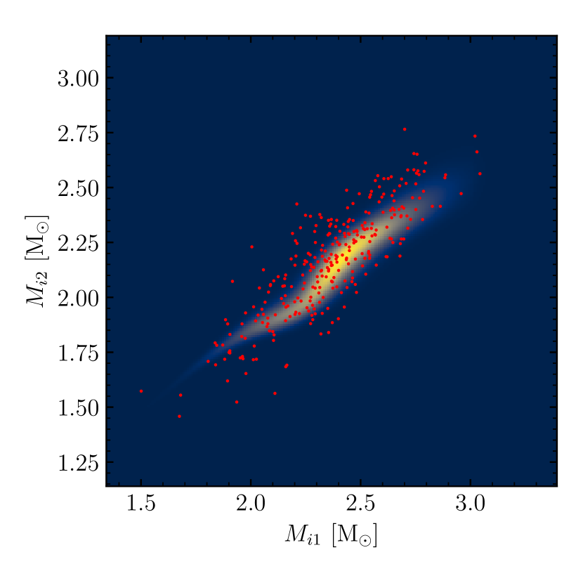
Figure 6: The likelihood given by Equation (5) in the $M_{i1}$-$M_{i2}$ plane, evaluated for WD J2007$-$3701AB and a 3-segment mock IFMR. The red points show 300 samples drawn from the joint-distribution of $M_{f1}$ and $M_{f2}$ and then converted to initial masses via the inverse IFMR. These samples are subsequently used to numerically integrate the likelihood function.

With a numerical recipe for calculating the integral in Equation (8), we have everything we need to calculate the total likelihood in Equation (3). All that remains to determine the posterior distribution on the IFMR, $P(\mathrm{IFMR}|\mathrm{DWDs})$ in Equation (2), is the prior distribution on the IFMR. In the following sub-sections, we introduce extensions to this framework. The priors on the associated hyper-parameters are defined therein. Specific choices of priors on the IFMR and their effects on the results are given in Section 5.

4.2 Dealing with outliers

While some systems in our sample (e.g. WD J2223$+$2201AB, Table LABEL:tab:dwds_fits) clearly cannot obey an IFMR (i.e. two stars that formed together, evolving independently), other outliers may be more subtle. It is therefore insufficient to cherry-pick a-priori a sub-sample of our double white dwarfs in order to fit the IFMR. Instead we have implemented a mixture model (Hogg et al., 2010) that naturally accounts for the presence of outliers.

We first consider the likelihood given for a double white dwarf where both components have evolved independently as single stars, i.e. Equation 5, which we now refer to as $L_{\mathrm{0}}$. For systems that have not followed this evolutionary path, e.g. due to mergers or additional mass loss, we make a simple modification to $L_{\mathrm{0}}$, instead assuming that the affected data have been drawn from a distribution with a wider variance than implied by the measured $\Delta\tau_{\mathrm{WD}}$. Therefore in the covariance matrix, $\Sigma$, we make the substitution $\sigma_{\mbox{$\Delta\tau_{\mathrm{WD}}$}}^{2}\mapsto\sigma_{\mbox{$\Delta\tau_{\mathrm{WD}}$}}^{2}+\sigma_{\mathrm{outlier}}^{2}$, where $\sigma_{\mathrm{outlier}}$ is a free parameter representing the additional uncertainty in the cooling age difference. We refer to this altered uncertainty as $L_{\mathrm{outlier}}$. Finally these separate likelihoods are combined into a single likelihood, $L_{\mathrm{total}}$, where

$$L_{\mathrm{total}}=(1-f_{\mathrm{outlier}})\times L_{\mathrm{0}}+f_{\mathrm{outlier}}\times L_{\mathrm{outlier}},$$ (10)

and where $f_{\mathrm{outlier}}$ is a free-parameter representing the fraction of systems in our sample that are outliers. This combined likelihood is used in all fits presented in later sections. In terms of priors, we used a uniform distribution on $f_{\mathrm{outlier}}$ in the range 0 to 1, and a uniform distribution on $\sigma_{\mathrm{outlier}}$ in the range 0 to 13.8 Gyr.

4.3 Dealing with underestimated uncertainties

Uncertainties for spectroscopic fitting of DA white dwarfs are generally assumed to be around a 1–2 per cent in $T_{\mathrm{eff}}$ and a few 0.01 dex in $\log g$ (Liebert et al., 2005; Voss et al., 2007). However, when fitting high quality spectra such as ours (especially with the additional constraint of Gaia photometry), the formal uncertainties on the results are often found to be much smaller than the numbers above. Our analysis in Section 5 is no exception with instances of $T_{\mathrm{eff}}$ uncertainties below $10$ K and $\log g$ errors of a few $0.001$ dex (Table LABEL:tab:dwds_fits).

The effect of ignoring such small uncertainties, is that the fitted IFMR may become overly constrained by a few systems. Furthermore, in practice we found that this led to some objects that would consistently yield a likelihood (Equation (4)) of zero which would propagate through to the total likelihood (Equation (3)). In the analysis of Andrews et al. (2015), the authors folded in $T_{\mathrm{eff}}$ relative uncertainties of 1.2 percent, and $\log g$ uncertainties of 0.038 dex according to Liebert et al. (2005). While we could indeed adopt these same external uncertainties and apply them to our analysis, we instead chose to estimate them as part of our fits to the IFMR, including the relative $T_{\mathrm{eff}}$ uncertainty and $\log g$ uncertainty as free parameters to be determined.

We implemented this in our model by adding these uncertainties in quadrature into the $T_{\mathrm{eff}}$-$\log g$ covariance matrices for each system, at each step in the fit. These were then converted to mass-$\Delta\tau_{\mathrm{WD}}$ covariance matrices via the mass-radius relations and cooling age calculations of Bédard et al. (2020).

To treat these extra parameters as part of our Bayesian framework also requires considering their prior distributions. With no other prior information, an uninformative Jeffreys prior can be used, i.e. $P(\sigma)\propto 1/\sigma$. Fortunately we do have such extra information, as WD J1336$-$1620AB was observed twice, with somewhat different results on the $T_{\mathrm{eff}}$ and $\log g$, exceeding the internal fitting errors.

For $N$ observations of a quantity $x$ ($\ln\mbox{$T_{\mathrm{eff}}$}$ or $\log g$) for both white dwarfs in a binary, we consider the case where the values of $x$ are drawn from normal-distributions with separate means ($\mu_{A}$ and $\mu_{B}$), but a shared dispersion $\sigma$. Therefore the likelihood of our data $\mathbf{x}$ is

$$L(\mathbf{x}|\mu_{A},\mu_{B},\sigma)\propto\prod_{i}^{N}\sigma^{-2}\exp\left(-\frac{(x_{A,i}-\mu_{A})^{2}}{2\sigma^{2}}-\frac{(x_{B,i}-\mu_{B})^{2}}{2\sigma^{2}}\right).$$ (11)

However, since we only care about the value of $\sigma$ we can marginalise over $\mu_{xA}$ and $\mu_{xB}$, yielding

$$L(\mathbf{x}|\sigma)\propto\sigma^{-2(N-1)}\exp\left(-\frac{S}{2\sigma^{2}}\right),$$ (12)

an inverse gamma-distribution in terms of $\sigma^{2}$ where

$$S=\sum_{i=1}^{N}\left[(x_{A,i}-\langle x_{A}\rangle)^{2}+(x_{B,i}-\langle x_{B}\rangle)^{2}\right],$$ (13)

and where $\langle x_{A}\rangle$ and $\langle x_{B}\rangle$ are the sample means. Setting $N=2$ and multiplying by the same Jeffreys prior as before transforms the likelihood into a posterior distribution on $\sigma$,

$$P(\sigma|\mathbf{x})\propto\sigma^{-3}\exp\left(-\frac{S}{2\sigma^{2}}\right),$$ (14)

which in turn can be used as prior distribution on the uncertainty parameters when fitting the IFMR.

For our systematic relative $T_{\mathrm{eff}}$ uncertainty ($\sigma_{T}$), and systematic $\log g$ uncertainty ($\sigma_{g}$), our measured values of WD J1336$-$1620AB led to $S_{T}=1.577\times 10^{-4}$. and $S_{g}=2.978\times 10^{-3}$. Consequently we found $\sigma_{T}=1.1_{-0.4}^{+1.1}$ per cent and $\sigma_{g}=0.046_{-0.018}^{+0.046}$ dex (median$\pm$16/84th percentiles), with 95 per cent highest density intervals of $0.3$–$4.0$ per cent and $0.015$–$0.172$ dex, respectively.

The median values for repeat observations of WD J1336$-$1620AB, are close to those reported by Liebert et al. (2005) (see above). Of course, systematic uncertainties in $T_{\mathrm{eff}}$ and $\log g$ can arise not only from the observations, but can also be stem from uncertainty in the models. These priors only estimate uncertainty from the former, but by allowing these additional variances to be free parameters, we allow additional sources of uncertainty to be accounted for in the posterior distribution, should the data support it.

4.4 IFMR functional form and parametrization

Thus far we have referred to the IFMR as some function, but without specifying its form, nor how it is parametrized. A natural choice of function is piece-wise linear, since it is easy to enforce monotonicity, as well as having a well defined inverse, and inverse gradient.

For an IFMR comprised of $N$ linear segments, this requires $N+1$ free parameters, though the specific parametrization is implementation specific. For example the first segment could be specified simply by a gradient and intercept, with subsequent segments specified only by a gradient. Most published IFMRs are given in this format or similar (e.g. Williams et al., 2009; Salaris et al., 2009; Cummings et al., 2018), with each linear segment expressed in $y=mx+c$ form. Andrews et al. (2015) used an alternative formulation in their analysis, specifying the angle of each segment makes in the $M_{i}$-$M_{f}$ plane, with a final free-parameter specifying the perpendicular distance the extrapolated first segment makes with the origin. In our analysis we simply chose to pre-specify a number of initial mass values, making the corresponding final-mass values the free parameters, with a similar approach also adopted by El-Badry et al. (2018). This choice makes it easy to check that the IFMR is monotonic, easy to invert the IFMR, and simple to calculate arbitrary values between break points (via linear interpolation).

Rather than restrict ourselves to a few segments, with the initial-mass values of the break points as free-parameters, we instead chose to use a much finer grid of fixed initial masses. This allowed us to sample the IFMR across the entire initial-mass range, thus permitting us to detect subtle features in the IFMR without imposing any expectation on where they should occur. Furthermore, this would allow us to detect which regions of the IFMR are well constrained by our data, and which regions remain uncertain.

After experimentation, we settled on an initial mass grid at 12 fixed values of initial mass (11 segments), with grid points placed at 0.75–1.5 $\mathrm{M}_{\odot}$ in 0.25 Msun steps, from 1.5–4.0 $\mathrm{M}_{\odot}$ in 0.50 $\mathrm{M}_{\odot}$ steps, from 4.0–6.0 $\mathrm{M}_{\odot}$ in 1.0 $\mathrm{M}_{\odot}$ steps, and with a final step at 8.0 $\mathrm{M}_{\odot}$. This grid is used throughout for the different fits described in the following subsections.

4.5 Pre-white dwarf lifetimes

The final ingredient required to constrain the IFMR is a relation between pre-white dwarf lifetimes and its dependence on initial-mass. For this purpose, we used model grids from MIST (MESA Isochrones & Stellar Tracks, Dotter, 2016; Choi et al., 2016) which themselves make use of MESA models (Modules for Experiments in Stellar Astrophysics, Paxton et al., 2011; Paxton et al., 2013, 2015, 2018). Specifically pre-white dwarf lifetimes were determined from the Zero Age Main Sequence (ZAMS) to the beginning of the Thermally-Pulsing AGB (TP-AGB), with Solar metallicity (i.e. [Fe/H] = 0), and $v/v_{\mathrm{crit}}=0.4$.

Metallicity is known to affect both the pre-white dwarf lifetime and amount of mass of mass loss occurring for a star of a given initial-mass (Meng et al., 2008), with higher metallicities resulting in increased mass loss (Romero et al., 2015). In cluster studies the progenitor metallicity can be determined from the metallicity of other cluster members, and indeed can be found to be non-Solar. While we cannot directly probe the metallicity for the progenitors of our DWD sample, these objects are disk stars and therefore can be expected to have had values close to Solar (Andrews et al., 2015). While some of the systems in our sample must have total ages of many Gyr, Rebassa-Mansergas et al. (2021) recently investigated the age-metallicity relation for a large sample of white dwarf-main sequence binaries, finding no dependence of metallicity on their ages. Therefore assuming Solar metallicity can be justified for the DWDs in our sample. Of course, stars in the disc show a spread in metallicity either side of Solar, however this represents a source of systematic uncertainty which we expect to be absorbed by the parameters in our extended Bayesian model.

4.6 Summary

Here we briefly summarise the differences between our framework and the original framework proposed by Andrews et al. (2015). Firstly Equation (5) accounts for parameter covariances between $M_{f1}$, $M_{f2}$, and $\Delta\tau_{\mathrm{WD}}$. This is particularly important for our fits, since the two spectra of each DWD were fit simultaneously assuming shared systematics. Even so, for systems with independent spectroscopic observations (i.e. $M_{f1}$ and $M_{f2}$ are determined independently), $\Delta\tau_{\mathrm{WD}}$ will necessarily covary with both masses, since cooling ages are sensitive to white dwarf masses.

Secondly, we make an important change to the importance sampling step. Andrews et al. (2015) chose to perform this integration over the space of pre-WD lifetimes (see their Equation 13). In our opinion this choice adds unnecessary computational effort, as the Jacobian will become the product of twice as many derivatives. By performing the integration over initial masses, as we have done in Equation (7), we eliminate the need to calculate the gradient of the pre-WD lifetime function. Subjectively, we also find the choice to integrate over initial-masses to be conceptually simpler, since one generally imagines pre-WD lifetime to be a function of the initial mass, rather than the other way around.

The other main differences to our model are the inclusions of outliers and unmodelled uncertainty in the $T_{\mathrm{eff}}$ and $\log g$ of our fits. These are already discussed in detail in the preceding subsections.

5 Results and discussion

5.1 A Monotonic IFMR

For our main investigation of the IFMR, we chose a simple set of constraints. Chiefly, we required the IFMR to be monotonic. This choice allowed us to apply the importance-sampling integral substitution in Equation 8, which relies on the IFMR having both a well defined inverse and inverse derivative.

In terms of other constraints, we only required the physically realistic restriction of fractional mass-loss between 0 and 1, and that total system ages were $<13.8$ Gyr (within the uncertainties). Specifically, we did not enforce the final mass free-parameters (on the IFMR) to be below the Chandrasekhar-limit. This is because, firstly, we would like to infer from our results at what initial-mass is the Chandrasekhar-limit reached (if at all). Secondly, our highest initial-mass point, at 8 $\mathrm{M}_{\odot}$, is somewhat arbitrary, but since we require the IFMR to be monotonic, limiting the final-mass points below 1.4 $\mathrm{M}_{\odot}$, will therefore push all preceding final-mass points down to lower values in an artificial way. Nevertheless, we will investigate the effect of such a choice in Section 5.2.

We sampled the posterior distribution of our model described in Section 4, again using emcee (Foreman-Mackey et al., 2013) to perform an MCMC. Due to the large number of free parameters (12 for the IFMR, plus 4 hyper-parameters), we used an ensemble of 1000 walkers. For the importance sampling, we used 10 000 samples per evaluation of the likelihood. We found that the fit converged in $\approx 10\,000$ steps though we continued to 15 000 steps to ensure a large number of samples could be obtained post burn-in.

Table 2: Table of results for our three IFMR fits. The parameters in rows 5 onward correspond to the fixed initial masses with the tabulated values corresponding to the final masses at that point in the IFMR. Fit 1 refers to our primary fit with a monotonic IFMR. Fit 2 includes an additional prior where final mass samples are restricted below $M_{\mathrm{Ch}}=1.4$ $\mathrm{M}_{\odot}$. Fit 3 instead includes the condition that mass-loss is also monotonic.

Parameter	Fit 1	Fit 2	Fit 3
$f_{\mathrm{outlier}}$	$0.59\pm 0.21$	$0.59_{-0.22}^{+0.23}$	$0.59_{-0.22}^{+0.21}$
$\sigma_{\mathrm{outlier}}$ [Gyr]	$0.70_{-0.22}^{+0.40}$	$0.69_{-0.23}^{+0.41}$	$0.72_{-0.23}^{+0.36}$
$\sigma_{T_{\mathrm{eff}}}$ [$\%$]	$1.36_{-0.63}^{+2.09}$	$1.34_{-0.62}^{+2.23}$	$1.38_{-0.65}^{+2.05}$
$\sigma_{\log g}$ [dex]	$0.049_{-0.006}^{+0.007}$	$0.049_{-0.006}^{+0.007}$	$0.049\pm 0.006$
$0.75$ $\mathrm{M}_{\odot}$	$0.297_{-0.204}^{+0.182}$	$0.295_{-0.200}^{+0.176}$	$0.485_{-0.050}^{+0.045}$
$1.00$ $\mathrm{M}_{\odot}$	$0.552_{-0.018}^{+0.015}$	$0.551_{-0.019}^{+0.015}$	$0.552_{-0.017}^{+0.015}$
$1.25$ $\mathrm{M}_{\odot}$	$0.595_{-0.013}^{+0.011}$	$0.594_{-0.012}^{+0.011}$	$0.594_{-0.012}^{+0.011}$
$1.50$ $\mathrm{M}_{\odot}$	$0.614_{-0.009}^{+0.008}$	$0.613_{-0.008}^{+0.009}$	$0.613_{-0.009}^{+0.009}$
$2.00$ $\mathrm{M}_{\odot}$	$0.632_{-0.011}^{+0.013}$	$0.631_{-0.011}^{+0.011}$	$0.630_{-0.010}^{+0.013}$
$2.50$ $\mathrm{M}_{\odot}$	$0.666_{-0.021}^{+0.027}$	$0.657_{-0.017}^{+0.024}$	$0.658_{-0.018}^{+0.024}$
$3.00$ $\mathrm{M}_{\odot}$	$0.727_{-0.031}^{+0.036}$	$0.711_{-0.030}^{+0.027}$	$0.711_{-0.030}^{+0.027}$
$3.50$ $\mathrm{M}_{\odot}$	$0.803_{-0.052}^{+0.056}$	$0.760_{-0.029}^{+0.040}$	$0.763_{-0.029}^{+0.034}$
$4.00$ $\mathrm{M}_{\odot}$	$0.861_{-0.032}^{+0.033}$	$0.835_{-0.041}^{+0.027}$	$0.828_{-0.045}^{+0.030}$
$5.00$ $\mathrm{M}_{\odot}$	$0.909_{-0.037}^{+0.134}$	$0.875_{-0.024}^{+0.026}$	$0.872_{-0.025}^{+0.026}$
$6.00$ $\mathrm{M}_{\odot}$	$1.236_{-0.290}^{+2.305}$	$0.912_{-0.032}^{+0.076}$	$0.909_{-0.030}^{+0.059}$
$8.00$ $\mathrm{M}_{\odot}$	$4.679_{-3.012}^{+2.311}$	$1.101_{-0.102}^{+0.172}$	$1.053_{-0.067}^{+0.107}$

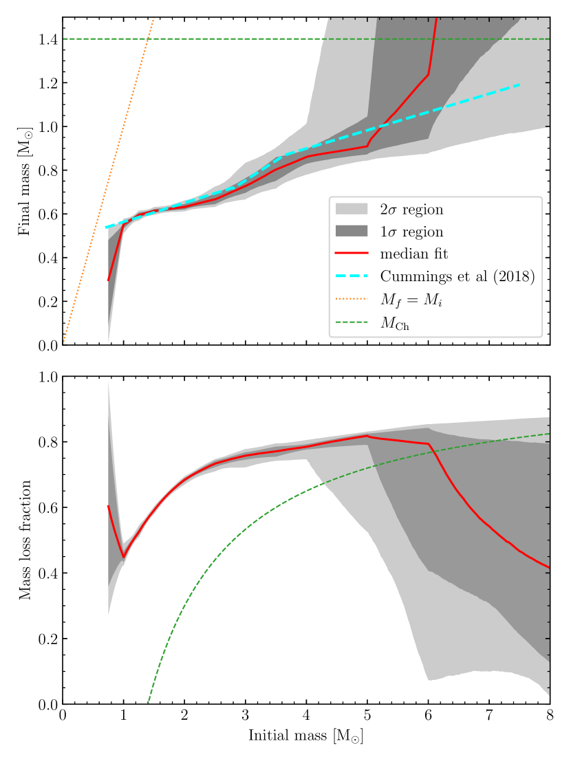
Figure 7: Our best fitting IFMR (red) from 0.75–8.0 $\mathrm{M}_{\odot}$, with the constraints that the IFMR is monotonic, and mass loss is bounded between 0 and 1 (Fit 1). Furthermore the presence of outliers and underestimated $T_{\mathrm{eff}}$ and $\log g$ uncertainties are accounted for. The $1\sigma$ and $2\sigma$ uncertainty regions are indicated by the medium and light grey areas, respectively. Good agreement with the IFMR of Cummings et al. (2018) to within $1\sigma$ is observed between 1–5 $\mathrm{M}_{\odot}$.

The resulting IFMR is shown in Figure 7, along with the mass-loss fraction occurring as a function of initial mass. This is compared with the IFMR from Cummings et al. (2018) (a wider comparison against other published IFMRs is performed in Section 5.5). All results are given in the Fit 1 column of Table 2. A corner plot of converged parameters is shown in Figure LABEL:fig:cornerFit1. In general we find good agreement between 1–5 $\mathrm{M}_{\odot}$, with extremely tight constraints for initial masses of 1–2 $\mathrm{M}_{\odot}$ with $M_{f}$ uncertainties of 0.01–0.02 $\mathrm{M}_{\odot}$. The steepening gradient occurs in broadly the same region as that found by Cummings et al. (2018), though we found this section of the IFMR to be somewhat wider being located at 2.5–4.0 $\mathrm{M}_{\odot}$ (compared with 2.85–3.60 $\mathrm{M}_{\odot}$ for Cummings et al. 2018). From 4–5 $\mathrm{M}_{\odot}$, we find our median result is flatter than Cummings et al. (2018), though still within our widening $1\sigma$ contour.

For initial-masses above 6.0 $\mathrm{M}_{\odot}$ we have virtually no constraint on the IFMR due to the absence of white dwarfs with final masses significantly above 1.0 $\mathrm{M}_{\odot}$ in our fitted sample. Specifically in the mass-loss panel, the MCMC samples are seen to have filled the entire available parameter space, subject to the condition of bounded mass-loss and a monotonic IFMR. Similarly, for initial masses below 1.0 $\mathrm{M}_{\odot}$ we have effectively no data covering this region, and so again the fit is very poor. This is most obvious in the mass-loss panel, demonstrating that a wide range of mass-loss fractions are covered by our $2\sigma$ contour at an initial mass of 0.75 $\mathrm{M}_{\odot}$.

For the hyper-parameters, firstly, we found a particularly large (though poorly constrained) $f_{\mathrm{outlier}}$ of $0.59\pm 0.21$, and with a corresponding $\sigma_{\mathrm{outlier}}$ of $0.70_{-0.22}^{+0.40}$ Gyr. The interpretation of $f_{\mathrm{outlier}}$ is discussed in more detail in Section 5.7, but essentially is constrained only by a few systems with high white dwarf masses. For the systematic uncertainty parameters, we found $\sigma_{\mbox{$T_{\mathrm{eff}}$}}=1.36_{-0.63}^{+2.09}$ per cent, and $\sigma_{\log g}=0.049_{-0.006}^{+0.007}$ dex. For $\sigma_{\mbox{$T_{\mathrm{eff}}$}}$, this remains similar to the prior distribution evaluated in Section 4.3, though with a slightly higher median value, and larger dispersion. For $\sigma_{\log g}$ on the other hand, the distribution was found to be almost Gaussian, with small uncertainty, indicating this parameter is particularly sensitive to our complete set of data. These values are in close agreement to the $\sigma_{\mbox{$T_{\mathrm{eff}}$}}=1.4$ per cent and $\sigma_{\log g}=0.042$ dex found by Genest-Beaulieu & Bergeron (2019). Converting these uncertainties into masses and cooling ages, we found that typical white dwarf mass errors of 0.03 $\mathrm{M}_{\odot}$, and cooling age relative uncertainties of 5–20 per cent. Importantly, for these four hyper-parameters, the corner-plot (Figure LABEL:fig:cornerFit1) shows no obvious covariance with the IFMR parameters, meaning small changes to the hyper-parameters do not strongly affect the IFMR itself.

5.2 Chandrasekhar mass limit

In the previous section, it is clear that our IFMR is poorly constrained for $M_{i}>5$ $\mathrm{M}_{\odot}$, due to an absence of data with $M_{f}>1.0$ $\mathrm{M}_{\odot}$. As a result, for $M_{i}$ in the range 5–8 $\mathrm{M}_{\odot}$, our posterior distribution easily fills the entire parameter space between our priors of a monotonic IFMR prior and mass loss fractions between 0 and 1. Naturally this means that many of the samples exceed the Chandrasekhar limit to an extreme degree.

Our code allows the Chandrasekhar-limit to easily be imposed as a prior on the $M_{f}$ values at each fixed $M_{i}$. We therefore repeated our fit to the IFMR with this extra constraint enforced. Because of the reduced phase-space our MCMC could explore, the model converged faster, only taking about 6000 steps, though we ran to 10 000 for the same reasons as before.

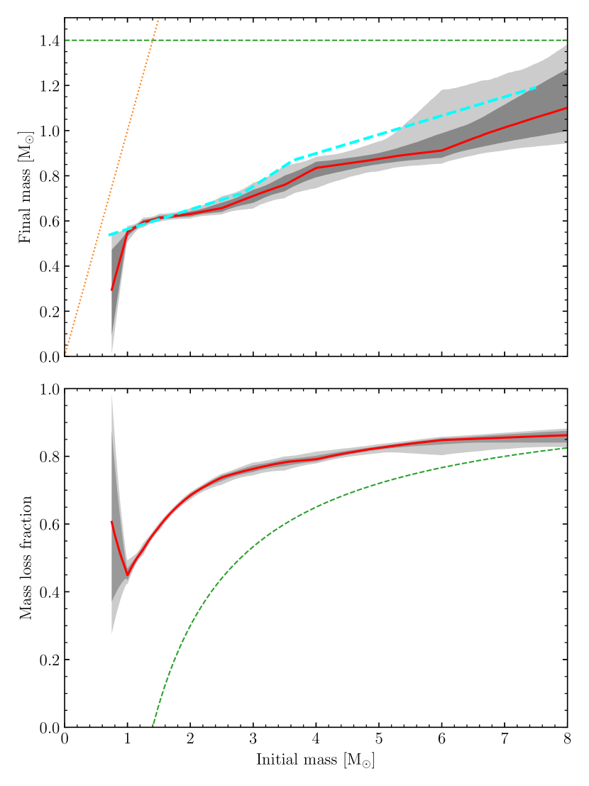
Figure 8: Our best fitting IFMR, including the additional constraint that all final mass points should be below 1.4 $\mathrm{M}_{\odot}$ (Fit 2). Figure elements have the same meaning as in Figure 7.

The resulting best fit is shown in Figure 8, and tabulated in column Fit 2 in Table 2. The four hyperparameters are virtually unchanged, with differences only seen for the IFMR final mass parameters. At the low mass end, where $M_{i}<2$ $\mathrm{M}_{\odot}$, essentially no difference is seen between this new IFMR and the one presented in Figure 7 (Fit 1). Of course, at the high mass end, where the IFMR was previously unconstrained, the $1\sigma$ and $2\sigma$ contours appear relatively tight with $M_{f}=1.101_{-0.102}^{+0.172}$ at $M_{i}=8$ $\mathrm{M}_{\odot}$. However, as predicted, this has also had an affect on the intermediate range. Because we have imposed a monotonic IFMR, forcing the high mass end to be below 1.4 $\mathrm{M}_{\odot}$, has by extension also pushed down the final mass values at intermediate initial masses by about $1\sigma$. The result is that this IFMR now disagrees with the Cummings et al. (2018) IFMR by more than $2\sigma$ between initial masses of 3.5–5.5 $\mathrm{M}_{\odot}$. We therefore recommend using the IFMR (Fit 1) over this one (Fit 2), and only for initial masses below 5 $\mathrm{M}_{\odot}$.

5.3 Monotonic mass loss

Inspecting Figure 7, it is apparent that over the well constrained range (1–5 $\mathrm{M}_{\odot}$), mass-loss also appears to be monotonic with respect to initial mass. This trend only breaks down at higher masses where we are unconstrained by data, and so our MCMC samples the entire parameter space. We therefore introduced the additional assumption that not only the IFMR is monotonic, but so also is mass-loss as a function of initial mass. To investigate the effect of imposing this restriction, we repeated the fit from Section 5.1, the same number of walkers (1000) and marginalisation samples (10 000) were used running for 10 000 steps. The only change compared to Fit 1 was that we imposed a prior constraining the mass loss fraction to also be monotonic.

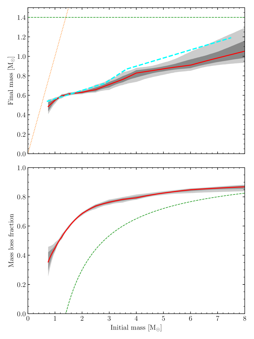
Figure 9: Our best fitting IFMR including the constraint that mass-loss is also monotonic with initial mass (Fit 3). Figure elements have the same meaning as in Figure 7.

The resulting IFMR is shown in Figure 9, and with the results tabulated as Fit 3. Compared to our results with non-monotonic mass-loss (Figure 7), the IFMR is pushed down substantially at the high-mass end (even more so than in Fit 2), with a final mass value of $1.06_{-0.07}^{+0.11}$ $\mathrm{M}_{\odot}$ at 8.0 $\mathrm{M}_{\odot}$. Therefore, an IFMR with this assumption is unable to produce near Chandrasekhar-mass white dwarfs through single-star evolution. Furthermore, between 3.0–6.5 $\mathrm{M}_{\odot}$, we find more than $2\sigma$ disagreement with the IFMR of Cummings et al. (2018), implying that the constraint of monotonic mass-loss is unlikely. Consequently it is possible that the mass-loss fraction does in fact peak somewhere between 5–8 $\mathrm{M}_{\odot}$. Evidently this result, and that of Fit 2, demonstrate that care must be taken when choosing priors, as these can have an unexpectedly large effect on the results.

At the low mass end, between 0.75–1.0 $\mathrm{M}_{\odot}$, this IFMR is more tightly constrained than in either Fit 1 or Fit 2, as IFMRs with high mass loss at low initial-mass are ruled out, with the median line appearing to tend towards 0. Although, very poorly constrained by our data (only our priors), this result is somewhat realistic as the lowest mass stars – all of which are still on the main sequence given their long lifetimes – will evolve directly into white dwarfs without significant mass-loss once their hydrogen fuel is depleted, due to the reduced ability or inability to ignite helium burning. Therefore, users of our results may wish to use the parameters from Fit 3 when estimating the initial masses of low mass white dwarfs, though these results are clearly unrealistic at higher masses, where parameters from Fit 1 should be used instead.

5.4 Non-monotonic IFMR

Although we restrict ourselves here to monotonic IFMRs only, we note that our code does permit non-monotonic IFMRs to be fitted. However, this requires changing the domain of integration from the final-final mass plane to the initial-initial mass plane, where it is not possible to restrict the area of integration to a region smaller than the whole plane up to 8 $\mathrm{M}_{\odot}$ for both components. Therefore in order to maintain precision of the integrals the number of integration samples should be increased by a factor 100 or more.

Given these computational requirements, we consider such a task beyond the scope of this work at present. However we note that recent work by Marigo et al. (2020) and Marigo et al. (2022) suggest that the IFMR may indeed be non-monotonic over a small mass range (1.8–2.2 $\mathrm{M}_{\odot}$), and may be responsible for the formation of carbon stars. A more detailed comparison with this result is given in the following section.

5.5 Comparison with other IFMRs

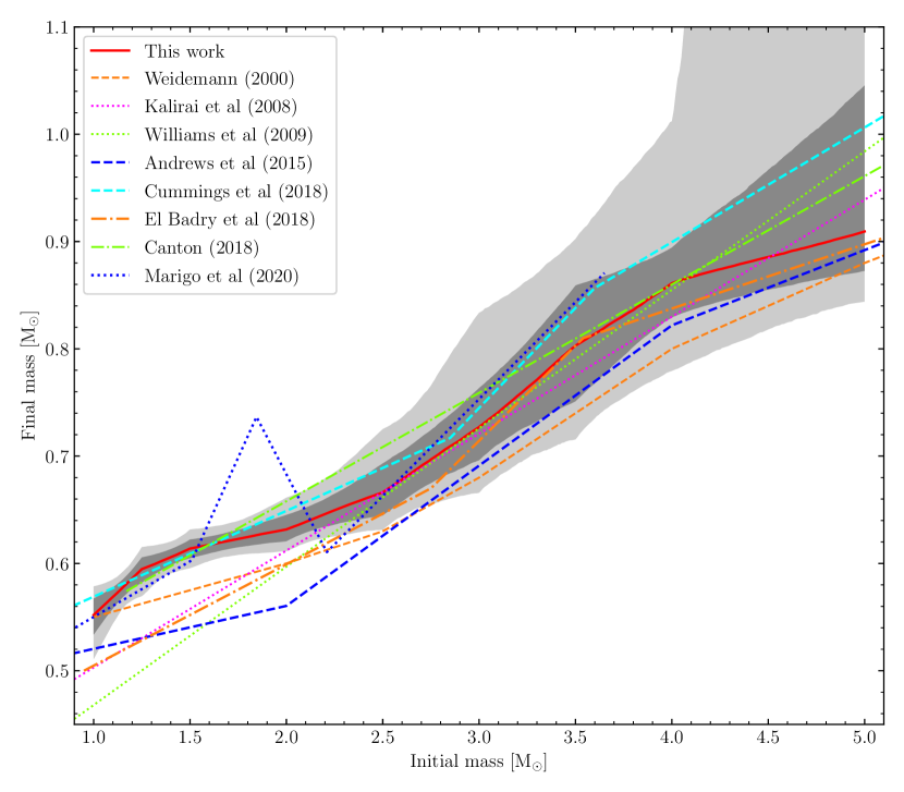
Figure 10: Comparison of our best fitting IFMR (Fit 1, red line) to those from other works, focusing on the range 1–5 $\mathrm{M}_{\odot}$. The grey regions have the same meaning as in Figure 7. Note that the uncertainties on the comparison IFMRs are not shown.

In Sections 5.1–5.3, we presented our different IFMR fits while providing a comparison only to the IFMR of Cummings et al. (2018). Of course many other works in recent years have presented other IFMRs, which we also wish to compare to. In Figure 10, we compare our best fitting results to a variety of published IFMRs over the range 1–5 $\mathrm{M}_{\odot}$, where our results are well constrained. This includes several cluster based IFMRs (Weidemann, 2000; Kalirai et al., 2008; Williams et al., 2009; Cummings et al., 2018; Canton, 2018), the Gaia population based IFMR of El-Badry et al. (2018), and the fiducial model of Andrews et al. (2015) using DWDs. As with our own IFMR, many of these works also make the assumption of a monotonic IFMR (El-Badry et al., 2018; Andrews et al., 2015), or are comprised of only a few linear segments and so do not result in negative gradients over the wide initial-mass range covered by each segment. We also show the non-monotonic IFMR of Marigo et al. (2020).

Over the range 2.5–5.0 $\mathrm{M}_{\odot}$, we observe agreement with all comparison IFMRs, within our 2$\sigma$ shaded region. Above initial masses of 3.0 $\mathrm{M}_{\odot}$, the comparison IFMRs show even better agreement, with the majority within the 1$\sigma$ shaded region. At these higher masses, we generally have less data to constrain the IFMR, so it is perhaps no surprise that we find the greatest agreement where our constraints are weakest. Even so, at $M_{i}=4.0$ $\mathrm{M}_{\odot}$, our final masses are still constrained to within $\pm 0.033$ $\mathrm{M}_{\odot}$.

The largest disagreement is observed between $1.0$–$2.5$ $\mathrm{M}_{\odot}$, depending on the IFMR. For the cluster results of Cummings et al. (2018) and Canton (2018), we continue to find reasonable agreement over this range, noting that the latter consists of a single linear relation. Compared to the other cluster IFMRs (Weidemann, 2000; Kalirai et al., 2008; Williams et al., 2009), we find final masses that are about 0.05 $\mathrm{M}_{\odot}$ higher. However, these are the oldest studies we show; the two more recent cluster analyses are consistent with our results, which we take that as a sign that our results are accurate in this range.

We also find a similar level of disagreement with the result of El-Badry et al. (2018), which was based on modelling the distribution of DA white dwarfs in the Gaia DR2 Hertzsprung-Russel diagram. At the low mass end, their IFMR has similar level of uncertainty reported, and closely follows the results of Kalirai et al. (2008) over the whole initial mass range shown.

Somewhat surprisingly, at $M_{i}=2.0$ $\mathrm{M}_{\odot}$, our results show the largest disagreement with Andrews et al. (2015), despite using the same general methodology. Even at higher masses, our results remain about $1\sigma$ above those of Andrews et al. (2015). Of course our results have benefited from a larger sample size, with parallaxes and precise photometry from Gaia DR3 also providing more accurate spectroscopic parameters. Since we have taken great care to account for sources of systematic uncertainties in both the spectroscopic fits and in the IFMR fitting, we expect that our IFMR ought to be more accurate, and with realistic uncertainties.

Finally we observe clear disagreement with Marigo et al. (2020), where their IFMR peaks near 1.8 $\mathrm{M}_{\odot}$. This non-monotonic IFMR was invoked following the discovery of cluster white dwarfs with low initial masses (1.6–2.1 $\mathrm{M}_{\odot}$). In particular, a white dwarf in NGC 752 was found with a lower final mass, but higher initial mass than members of R-147 and NGC 7789, implying a downwards trend in the IFMR, before turning upwards again. Since our fits assume a monotonic IFMR as a prior, our model cannot reproduce this feature. However, if the IFMR kink was present in our sample, we would expect our resulting IFMR to have been forced upwards through the middle of the triangular feature, rather than across its base. This is especially true, given that the 0.6–0.75 $\mathrm{M}_{\odot}$ range in final masses is covered by a large fraction of our DWD sample (Figure 4). Given that the work by Marigo et al. (2020) required observations of particularly old clusters, we can only speculate that those cluster members may not be representative of the disk stars in our analysis. As discussed in Section 5.4, in principle our code has the ability to fit non-monotonic IFMRs, but at greatly increased computational cost, opening up the possibility to investigate the reported IFMR kink with a larger number of DWDs in the future.

5.6 Determining progenitor masses of white dwarfs

We consider the common case of deriving progenitor masses from the masses of isolated white dwarfs and an IFMR. The simplest approach is to draw normally distributed samples of the white dwarf mass from a measurement and its uncertainty, and then use the inverse-IFMR to determine the corresponding initial mass. This can be repeated over all IFMR samples to account for uncertainty in the IFMR.

A better alternative is to consider the likelihood of a final mass, given its uncertainty, an initial mass, and an IFMR,

$$P(M_{f}|\mathrm{IFMR},M_{i},\sigma_{M_{f}})\propto\frac{1}{\sigma_{M_{f}}}\exp\left(-\frac{1}{2}\left[\frac{M_{f}-\mathrm{IFMR}(M_{i})}{\sigma_{M_{f}}}\right]^{2}\right).$$ (15)

This likelihood can be turned into a posterior distribution on $M_{i}$ by multiplying by a prior distribution on $M_{i}$. In the absence of data to constrain $M_{i}$, the only assumption that can be made is that the star was drawn from the mass distribution of all main sequence stars, i.e. the IMF. We therefore adopt the high-mass part of the IMF (valid for $M_{i}>0.5$ $\mathrm{M}_{\odot}$) as a prior, so that $P(M_{i})\propto M_{i}^{-2.3}$ and

$$P(M_{i}|\mathrm{IFMR},M_{f},\sigma_{M_{f}})\propto M_{i}^{-2.3}P(M_{f}|\mathrm{IFMR},M_{i},\sigma_{M_{f}}).$$ (16)

However, this distribution depends on a specific IFMR (as opposed to a distribution of IFMRs), and so we must marginalise over the entire space of IFMRs, i.e. samples from the posterior in Section 5.1. Numerically, this equates to taking the arithmetic mean over IFMR samples

$$P(M_{i}|M_{f},\sigma_{M_{f}})=\frac{1}{N}\sum_{k}^{N}P(M_{i}|\mathrm{IFMR}_{k},M_{f},\sigma_{M_{f}}),$$ (17)

where the summand must be normalised over the range 0.75 to 8 $\mathrm{M}_{\odot}$, to provide correct weighting over each $P(M_{i}|\mathrm{IFMR}_{k},M_{f},\sigma_{M_{f}})$. Since the resulting distribution is one dimensional, it is simple to draw $M_{i}$ samples from the posterior without resorting to more complex methods such as MCMC.

Posterior distributions from our Bayesian approach are shown in Figure 11, using a final mass uncertainty of 0.03 $\mathrm{M}_{\odot}$ (typical for our DWD sample, when systematic uncertainties are accounted for). The distributions for $M_{f}=0.6$ and $0.7$ $\mathrm{M}_{\odot}$, appear particularly well-behaved given that they correspond to the most tightly constrained part of our IFMR. While the distributions for $M_{f}=0.8$ and $0.9$ $\mathrm{M}_{\odot}$ appear further from normal, they are still adequate to determine 16th, 50th, and 84th percentiles and draw conclusions about the initial mass. For $M_{f}=1.0$ $\mathrm{M}_{\odot}$, sharp features appear in the posterior, resulting from a lack of constraining data, and poor sampling by our IFMR break points. We therefore recommend using our IFMR results over the range $0.53$–$0.95$ $\mathrm{M}_{\odot}$ (for lower masses, the implied median pre-WD lifetimes exceed the age of the universe).

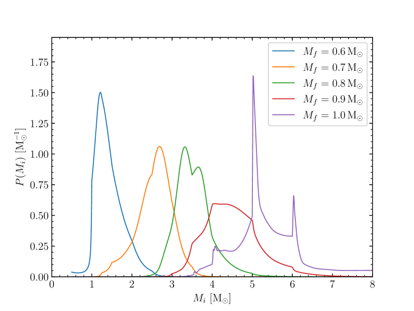
Figure 11: Posterior distributions of initial mass for a range of final masses, and with assumed final mass uncertainties of $0.03$ $\mathrm{M}_{\odot}$. Marginalisation over IFMRs uses the final MCMC step of our fit in Section 5.1, with 1000 samples.

In comparison to the simple approach described earlier, we found the Bayesian approach yields more robust results. For example, using $M_{f}=0.60\pm 0.03$ $\mathrm{M}_{\odot}$, the simple approach gives $M_{i}=1.34_{-0.23}^{+0.67}$ $\mathrm{M}_{\odot}$, which is similar to the $1.36_{-0.24}^{+0.42}$ $\mathrm{M}_{\odot}$ found for the Bayesian method (Figure 11), but with slightly worse uncertainty. However, inspecting the distribution of $M_{i}$ samples, the simple approach also shows spikes or discontinuities at each break point in the IFMR (similar to what is seen for $M_{f}=1.0$ $\mathrm{M}_{\odot}$ in Figure 11), which are not present for the Bayesian approach in this mass range. We provide a tool within our python package for calculating these distributions from white dwarf masses.

We conclude by noting that Equation 15 relies on the IFMR only in the foward direction, making no reference to the inverse-IFMR, and so this approach is equally valid for non-monotonic IFMRs. While the resulting $M_{i}$ distribution will inevitably be multi-modal, these modes will be weighted by the IMF.

5.7 Initial masses and outlier probabilities for double white dwarfs

Within our Bayesian framework for fitting the IFMR (Section 4), we marginalised over initial masses in order to keep the number of free parameters to an acceptable level. However, it is still possible to calculate these after the fit. However, we cannot simply apply the methodology from Section 5.6 to each component separately. Firstly because $M_{i1}$ and $M_{i2}$ may have correlated uncertainties, secondly because we also have the constraint on cooling ages and their difference, and thirdly because we must consider the effect of the derived hyper-parameters on our sample.

To account for these caveats, we modify Equation 17 to

$$P(M_{i1},M_{i2}|\mathrm{DWD},\Sigma)=\frac{1}{N}\sum_{k}^{N}P(M_{i1},M_{i2}|\theta_{k},\mathrm{IFMR}_{k},\mathrm{DWD},\Sigma),$$ (18)

where $\theta_{k}$ is a vector of hyperparameters, and $\Sigma$ is the covariance matrix of the DWD parameters. We use the same $M_{f}$ priors and likelihood as in Sections 4 and 4.2. While the resulting distribution is now 2D, it is still possible to sample the $M_{f1}$-$M_{f2}$ plane on a fine grid, and calculate the posterior probability at each point. $M_{i1}$-$M_{i2}$ samples can then be drawn from this grid weighted according to the posterior. We give results for the estimated $M_{i1}$, $M_{i2}$ values and their covariance in Table LABEL:tab:m_tau_p.

Similarly, we can determine the probability that a specific DWD from our sample is an outlier, $P_{\mathrm{outlier}}$, after having fitted our IFMR. This requires converged samples of the IFMR and the hyper-parameters, $\theta$, from our fit. For each sample we calculate the outlier likelihood, $L_{\mathrm{outlier}}$ and the total likelihood $L_{\mathrm{total}}$ (defined according to Equation (10)), but where both likelihoods have been marginalised over the $M_{i1}$-$M_{i2}$ plane (using importance sampling from Section 4). Finally, to determine the probability that a specific system is an outlier, we simply require marginalising over our samples of fitted parameters according to

$$P_{\mathrm{outlier}}=\frac{1}{N}\sum_{k}^{N}\frac{f_{\mathrm{outlier},k}\times L_{\mathrm{outlier}}(\mathrm{DWD}|\theta_{k},\mathrm{IFMR}_{k},\Sigma)}{L_{\mathrm{total}}(\mathrm{DWD}|\theta_{k},\mathrm{IFMR}_{k},\Sigma)},$$ (19)

where $f_{\mathrm{outlier}}$ is the hyper-parameter corresponding to the fraction of systems that are outliers. These $P_{\mathrm{outlier}}$ will have values close to 1, if the two components in a system are not coeval, i.e. $\mbox{$\Delta\tau_{\mathrm{WD}}$}\neq-\mbox{$\Delta\tau_{\mathrm{preWD}}$}$ considering the uncertainties on both $\Delta\tau_{\mathrm{WD}}$ and $\Delta\tau_{\mathrm{preWD}}$. This necessarily means that we require high precision on both $\Delta\tau_{\mathrm{WD}}$ and $\Delta\tau_{\mathrm{preWD}}$ in order to be confident that a system is an outlier, or that both its components are coeval. We provide our estimate for $P_{\mathrm{outlier}}$ in Table LABEL:tab:m_tau_p.

The first thing to notice is that the vast majority of systems have $P_{\mathrm{outlier}}$ within one per cent of the mean value of $f_{\mathrm{outlier}}$. This is because for most systems, the uncertainty on the observed $\Delta\tau_{\mathrm{WD}}$ dominates the 0.7 Gyr of additional variance found for outlier systems (particularly once the systematics on $T_{\mathrm{eff}}$ and $\log g$ are considered), and so our methodology cannot confidently conclude whether additional variance is required. This begs the question of how $f_{\mathrm{outlier}}$ should be interpreted, and why its value is so high.

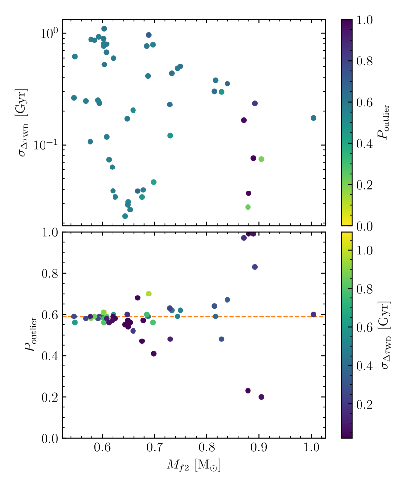
Figure 12: Outlier probabilities as for our 52 DWDs used to fit the IFMR. This is shown as a function of the mass of the heaviest component in the binary, $M_{f2}$, and the uncertainty in the cooling age difference (including $T_{\mathrm{eff}}$ and $\log g$ systematics), $\sigma_{\Delta\tau_{\mathrm{WD}}}$. In the bottom panel, $P_{\mathrm{outlier}}$ and $\sigma_{\Delta\tau_{\mathrm{WD}}}$ are inverted, and the median value of $f_{\mathrm{outlier}}$ is shown by the dashed orange line.

We demonstrate where this outlier probability arises from in Figure 12, where we show the outlier probabilities for each system as a function of the more massive white dwarf in the pair, $M_{f2}$, and the uncertainty on $\Delta\tau_{\mathrm{WD}}$  with assumed $T_{\mathrm{eff}}$ and $\log g$ systematic uncertainties of 1.4 per cent and 0.052 dex included, respectively. Across most of the parameter space, the $P_{\mathrm{outlier}}$ are almost identical to the central value found for $f_{\mathrm{outlier}}$ (0.59). Only six systems stand out from the crowd. These are WD J0101$-$1629AB, WD J1215$+$0948AB WD J2115$-$0741AB, and WD J2223$+$2201AB with high $P_{\mathrm{outlier}}$; and WD J1313$+$2030AB and WD J1336$-$1620AB with low $P_{\mathrm{outlier}}$. Inspecting the parameters of the high outlier probability systems it is easy to see how this classification was made, for example WD J0101$-$1629AB, the more massive component has been cooling for about 490 Myr, whereas the lower mass companion has a cooling age of 720 Myr – the inverse of what is expected for two white dwarfs born at the same time, but evolving independently as single stars.

All six of these systems (confident outliers, and confident non-outliers) have one thing in common: the masses of the heavier component, which are all between $0.87$–$0.91$ $\mathrm{M}_{\odot}$. While objects resulting from mergers are expected in this mass range, this does not explain why the most confident non-outliers are also found here. It is certainly true that for the more massive systems, the $\Delta\tau_{\mathrm{WD}}$ uncertainties appear substantially smaller, with 240 Myr for the worst of the six (WD J1215$+$0948AB). Instead we speculate that only for higher masses do we have enough precision on both $\Delta\tau_{\mathrm{WD}}$ and $\Delta\tau_{\mathrm{preWD}}$ to make any distinction between outliers and non-outliers. Therefore the outlier fraction for all systems, $f_{\mathrm{outlier}}$ is largely down to this small subset of six leading to such a high (and poorly constrained) value of $0.59_{-0.21}^{+0.22}$. Inspecting the bottom panel of Figure 12, we note that a few systems also show slightly more distinct $P_{\mathrm{outlier}}$ (both above and below 0.59) for white dwarf masses near 0.7 $\mathrm{M}_{\odot}$. At this mass range though, the balance is slightly towards systems with lower outlier probabilities.

For the four high $P_{\mathrm{outlier}}$ systems, even if there is a selection bias towards high outlier/non-outlier confidence near 0.9 $\mathrm{M}_{\odot}$, we conclude that the massive components in those four systems are candidate merger products from within former hierarchical triple systems. To rule out an alternative hypothesis of binaries formed via captures in multi-star interactions, we looked at the distribution of $P_{\mathrm{outlier}}$ against projected sky separation. All four high probability outliers are separated by only 400–1200 au making captured binaries extremely unlikely, and lending further weight to our explanation of mergers. The widest system in our fitted sample, WD J2351$-$1601AB at $27\,600\pm 700$ au, does have a slightly high $P_{\mathrm{outlier}}$ of 0.68, raising the prospect that this system could have formed via a capture event.

This approach to outlier probabilities provided one final opportunity to investigate the possibility of a non-monotonic IFMR as identified by Marigo et al. (2020). We generated synthetic binaries with initial masses and system ages covering a wide range of values. These were converted to final masses using the IFMR of Marigo et al. (2020), and the pre-WD lifetimes (and hence cooling ages) calculated from the same MIST models as before. We then determined the outlier probabilities using the same method as above (i.e. using our own IFMR results to make this determination). We found that the outlier probability could be maximised by placing the component with lower initial mass at the peak of the Marigo et al. (2020) IFMR, i.e. at $M_{i}=1.85\,\mbox{$\mathrm{M}_{\odot}$}$, while also requiring short cooling ages to reduce the uncertainties on $\Delta\tau_{\mathrm{WD}}$. With the initial mass of the other component $\geq 2.10\,\mbox{$\mathrm{M}_{\odot}$}$, we were able to produce outlier probabilities of $\simeq 0.90$ (though we were unable to produce the $\geq 0.97$ probabilities found for our most extreme outliers), demonstrating that our methodology can be sensitive to outliers produced by a non-monotonic IFMR.

As a final exercise we selected systems from our sample with both component masses between 0.6–0.75 $\mathrm{M}_{\odot}$ (Table LABEL:tab:dwds_fits), i.e. covering initial masses of 1.5–3.0 $\mathrm{M}_{\odot}$ from the Marigo et al. (2020) IFMR, and with at least one of the cooling ages below 300 Myr. This selection yielded 12 systems, all with outlier probabilities (Table LABEL:tab:m_tau_p) close to the median of 0.59, with the highest two values at 0.62 (WD J0120$-$1622AB and WD J0309$+$1505AB). Since these systems do not have outlier probabilities well above the 0.59 median or approaching the 0.90 found from our synthetic systems, we conclude that our IFMR and DWD sample do not provide evidence for a non-monotonic IFMR.

6 Conclusions and future work

We observed 90 DWDs using FORS2 spectroscopy. Of these, we were able to use 52 DA+DA, DA+DC, and DC+DC pairs to constrain the IFMR assuming a monotonic piecewise-linear functional form. Furthermore we were able to do this including the contribution of un-modelled uncertainties in their $T_{\mathrm{eff}}$ and $\log g$, while also establishing that several systems in our sample are outliers, potentially suggesting the mergers taking place within former hierarchical triple systems.

While the vast majority of our binary sample can be fitted well with hydrogen dominated model spectra, some of the white dwarfs clearly have helium dominated atmospheres, with the most obvious of these having DB and DZ spectral classifications. Additionally some DC white dwarfs, while at first ambiguous, turned out to incompatible with a hydrogen dominated atmosphere at the derived temperature (i.e. hydrogen Balmer lines would otherwise have been present). In the future, we intend to also include these systems by fitting models with helium dominated atmospheres instead. However, it should be noted that a first investigation of the IFMR for hydrogen-poor white dwarfs suggests that these objects have higher mass progenitors, i.e. that they follow a separate IFMR altogether (Barnett et al., 2021)

Looking further ahead, our sample is still relatively small, containing only 52 pairs used to constrain the IFMR, and only for final masses up to 1.0 $\mathrm{M}_{\odot}$. This means that our IFMR is only well constrained for initial masses below $5$–$6$ $\mathrm{M}_{\odot}$. Above that range, our fits merely reflect our choice of priors. Of course, identifying “well behaved” systems containing ultra-massive white dwarfs where both components are non-magnetic DAs, presents its own observational challenges. Fortunately, the entire Gaia white dwarf sample contains over 1200 wide pairs – more than an order of magnitude increase over the 90 we have observed so far. Over the next decade, many of these will be observed in multi-fibre spectroscopic surveys such as WEAVE, DESI, SDSS V, and 4MOST. Taking advantage of these upcoming systems will allow us to constrain the IFMR to even greater precision in the future.

A caveat to our implementation of the Bayesian framework is the time-complexity. Naïvely, Equation (3) implies a linear time-complexity in the number of white dwarfs, $N$, i.e. $\mathcal{O}(N)$. However, the importance sampling step to calculate the integral in Equation (8) limits the relative precision of this quantity for each DWD. Therefore, to maintain a constant relative precision in the total likelihood (Equation (3)), the number of integration samples (per system) must also increase linearly with $N$, increasing the overall time complexity to $\mathcal{O}(N^{2})$. For our fitted sample of $N=52$, this does not currently pose an issue, with the main IFMR fit taking a few days on a modern 10-core desktop machine, but will become problematic for samples with $N>100$. Therefore, alternative integration techniques that can reduce this time complexity should be investigated in advance of the large number of systems that will be observed in the coming years.

Data Availability

The spectroscopic data obtained in this work can be found from the ESO Science Archive Facility with Program IDs 0103.D-0718 and 109.231B. The MCMC chains from our IFMR fits will be made available alongside our python package, and also available upon reasonable request to the authors.

Appendix A Additional tables and figures

Table 3: Coordinates, spectral types (SpT), and Gaia DR3 data for our entire DWD sample that were followed up with FORS2. The “run(s)” column specifies which observing run (or runs) each DWD was observed in.

WD J	J2016 coordinates	SpT	parallax [mas]	$G$ [mag]	$B_{p}$ [mag]	$R_{p}$ [mag]	run(s)
0002$+$0733A	00:02:16.07$+$07:33:49.3	DAH	12.349±0.138	17.946±0.003	18.098±0.013	17.707±0.015	C
0002$+$0733B	00:02:15.27$+$07:33:58.5	DA	12.115±0.121	17.724±0.003	17.897±0.013	17.445±0.011
0007$-$1605A	00:07:34.39$-$16:05:14.1	DC	12.526±0.547	19.942±0.005	20.593±0.086	19.241±0.054	C
0007$-$1605B	00:07:35.02$-$16:05:32.6	DA	12.337±0.045	16.152±0.003	16.162±0.004	16.157±0.008
0022$-$7232A	00:22:29.86$-$72:32:08.5	DAZ	11.251±0.088	17.686±0.003	17.817±0.009	17.461±0.014	E
0022$-$7232B	00:22:33.21$-$72:32:32.6	DC	11.178±0.254	19.419±0.004	19.867±0.060	18.900±0.033
0023$+$0643A	00:23:36.32$+$06:43:20.2	DA	8.458±0.094	17.416±0.003	17.474±0.007	17.346±0.011	E
0023$+$0643B	00:23:35.64$+$06:43:25.2	DA	8.839±0.172	18.448±0.003	18.624±0.016	18.158±0.024
0052$+$1353A	00:52:12.26$+$13:53:01.4	DA	4.208±0.128	17.812±0.003	17.753±0.011	17.983±0.022	C
0052$+$1353B	00:52:12.72$+$13:53:00.5	DA	4.196±0.230	18.836±0.004	18.906±0.022	18.837±0.043
0059$-$2417A	00:59:09.54$-$24:17:28.5	DA	9.814±0.171	17.805±0.003	17.920±0.009	17.654±0.012	C
0059$-$2417B	00:59:09.29$-$24:17:33.4	DB	9.766±0.093	16.757±0.003	16.740±0.005	16.795±0.008
0101$-$1629A	01:01:31.47$-$16:29:09.7	DA	5.383±0.175	18.444±0.003	18.435±0.017	18.508±0.033	C
0101$-$1629B	01:01:31.05$-$16:29:08.7	DA	5.586±0.206	18.679±0.003	18.747±0.019	18.546±0.027
0104$+$2120A	01:04:57.72$+$21:20:10.5	DC	30.804±0.114	17.799±0.003	18.376±0.026	17.125±0.013	E
0104$+$2120B	01:04:56.23$+$21:19:52.0	DC	30.658±0.110	17.701±0.003	18.125±0.016	17.120±0.009
0109$-$1042A	01:09:04.41$-$10:42:15.8	DC	16.765±0.225	18.732±0.003	19.188±0.022	18.095±0.019	C
0109$-$1042B	01:09:03.60$-$10:42:14.6	DA	16.463±0.067	16.602±0.003	16.721±0.004	16.388±0.005
0120$-$1622A	01:20:58.81$-$16:22:47.3	DA	12.853±0.041	15.838±0.003	15.803±0.004	15.935±0.005	C
0120$-$1622B	01:20:59.33$-$16:22:48.9	DA	12.784±0.192	18.803±0.003	19.118±0.023	18.357±0.025
0215$+$1821A	02:15:23.76$+$18:21:15.4	DA	6.803±0.302	19.180±0.004	19.285±0.044	19.128±0.053	C
0215$+$1821B	02:15:24.11$+$18:21:28.8	DA	7.138±0.058	16.226±0.003	16.134±0.005	16.438±0.008
0220$-$1532A	02:20:30.98$-$15:32:47.8	DAH	12.841±0.142	18.173±0.003	18.298±0.022	17.911±0.026	E
0220$-$1532B	02:20:31.39$-$15:32:48.7	DA	12.758±0.169	18.446±0.003	18.591±0.037	18.080±0.025
0224$-$4611A	02:24:40.35$-$46:11:33.6	DAH	8.321±0.090	18.090±0.003	18.124±0.010	18.099±0.018	C
0224$-$4611B	02:24:40.72$-$46:11:40.3	DA	8.271±0.061	17.412±0.003	17.428±0.006	17.438±0.009
0225$-$1756A	02:25:56.42$-$17:56:14.9	DZ	14.738±0.086	17.360±0.003	17.468±0.008	17.145±0.010	C
0225$-$1756B	02:25:56.24$-$17:56:08.3	DA	14.900±0.133	18.155±0.003	18.444±0.014	17.729±0.013
0240$-$3248A	02:40:52.09$-$32:48:12.8	DAH	16.123±0.090	17.588±0.003	17.750±0.007	17.308±0.013	E
0240$-$3248B	02:40:51.75$-$32:48:35.9	DA	16.312±0.086	17.520±0.003	17.634±0.006	17.292±0.008
0253$-$6152A	02:53:39.41$-$61:52:52.3	DC	18.191±0.112	18.503±0.003	19.010±0.024	17.910±0.016	C
0253$-$6152B	02:53:41.86$-$61:52:15.7	DA	18.139±0.053	17.253±0.003	17.472±0.007	16.897±0.007
0309$+$1505A	03:09:53.83$+$15:05:10.1	DA	12.431±0.172	18.435±0.003	18.661±0.029	18.045±0.026	C
0309$+$1505B	03:09:53.89$+$15:05:20.4	DA	12.263±0.045	15.211±0.003	15.121±0.004	15.409±0.005
0344$+$1509A	03:44:11.51$+$15:09:45.2	DAH	18.524±0.076	16.808±0.003	16.934±0.006	16.592±0.006	C
0344$+$1509B	03:44:10.93$+$15:10:21.7	DA	18.367±0.062	16.450±0.003	16.566±0.006	16.229±0.010
0410$-$1641A	04:10:24.97$-$16:41:51.5	DA	9.837±0.047	15.481±0.003	15.375±0.004	15.687±0.005	C
0410$-$1641B	04:10:26.53$-$16:41:43.6	DA	9.863±0.048	16.356±0.003	16.326±0.004	16.477±0.006
0510$+$0438A	05:10:13.53$+$04:38:53.5	DA	20.127±0.039	15.376±0.003	15.383±0.008	15.380±0.006	C
0510$+$0438B	05:10:13.95$+$04:38:36.9	DA	20.218±0.036	14.226±0.003	14.137±0.003	14.420±0.004
0855$-$2637A	08:55:50.66$-$26:37:47.1	DA	18.810±0.059	16.923±0.003	17.043±0.007	16.738±0.010	A
0855$-$2637B	08:55:50.99$-$26:37:52.1	DA	18.725±0.055	16.767±0.003	16.905±0.007	16.529±0.007
0902$-$3540A	09:02:32.10$-$35:40:43.8	DAH	6.944±0.120	18.252±0.003	18.163±0.017	18.460±0.032	A
0902$-$3540B	09:02:30.88$-$35:40:38.9	DA	6.871±0.077	17.415±0.003	17.338±0.011	17.463±0.014
0920$-$4127A	09:20:16.14$-$41:27:11.1	DA	11.273±0.072	17.576±0.003	17.711±0.008	17.364±0.007	D
0920$-$4127B	09:20:16.07$-$41:27:03.7	DA	11.226±0.073	17.589±0.003	17.719±0.009	17.380±0.008
1006$+$0712A	10:06:23.12$+$07:12:11.6	DA	18.331±0.058	15.981±0.003	16.065±0.006	15.859±0.006	A
1006$+$0712B	10:06:23.21$+$07:11:53.2	DC	18.152±0.225	18.645±0.004	19.206±0.050	17.990±0.028
1014$+$0305A	10:14:01.72$+$03:05:48.8	DC	20.689±0.194	18.035±0.003	18.478±0.023	17.447±0.027	D
1014$+$0305B	10:13:59.96$+$03:05:52.3	DC	20.135±0.244	18.089±0.003	18.541±0.016	17.478±0.020
1015$+$0806A	10:15:01.43$+$08:06:13.8	DC	33.916±0.143	17.491±0.003	18.056±0.019	16.771±0.012	A
1015$+$0806B	10:15:02.30$+$08:06:38.3	DA	33.912±0.059	15.919±0.003	16.142±0.006	15.539±0.005
1019$+$1217A	10:19:54.59$+$12:17:17.7	DA	9.392±0.078	16.867±0.003	16.881±0.008	16.897±0.009	A
1019$+$1217B	10:19:55.88$+$12:16:31.2	DA	9.392±0.052	15.763±0.003	15.672±0.005	15.960±0.006
1100$-$1600A	11:00:21.84$-$16:00:15.9	DC	21.859±0.120	17.912±0.003	18.270±0.020	17.363±0.018	D
1100$-$1600B	11:00:22.83$-$16:00:12.7	DA	22.000±0.112	17.616±0.003	17.896±0.013	17.186±0.012
1124$-$1234A	11:24:07.17$-$12:34:42.7	DC	16.061±0.150	18.260±0.003	18.614±0.024	17.794±0.021	A
1124$-$1234B	11:24:05.37$-$12:34:44.9	DA	15.896±0.065	16.647±0.003	16.786±0.006	16.442±0.007
1159$-$4630A	11:59:41.71$-$46:30:34.2	DC	16.279±0.241	19.150±0.004	19.723±0.040	18.514±0.019	D
1159$-$4630B	11:59:56.83$-$46:29:03.3	DAH	15.943±0.096	17.436±0.003	17.590±0.007	17.163±0.010
1211$-$4551A	12:11:04.93$-$45:51:46.8	DA	8.061±0.122	17.907±0.003	18.007±0.008	17.747±0.013	D
1211$-$4551B	12:11:03.78$-$45:51:51.9	DA	8.217±0.202	18.716±0.003	18.917±0.031	18.286±0.030
1215$+$0948A	12:15:09.68$+$09:48:47.3	DA	10.177±0.129	17.921±0.003	18.014±0.011	17.858±0.016	B
1215$+$0948B	12:15:10.11$+$09:48:36.6	DA	10.462±0.126	17.773±0.003	17.898±0.009	17.576±0.011
1254$-$0218A	12:54:58.53$-$02:18:08.5	DA	8.373±0.541	19.549±0.005	19.795±0.039	19.104±0.049	A
1254$-$0218B	12:54:58.07$-$02:18:38.6	DA	7.954±0.080	16.635±0.003	16.594±0.006	16.759±0.008
1310$-$3930A	13:10:46.14$-$39:30:41.8	DA	6.751±0.200	18.729±0.004	18.709±0.041	18.735±0.035	D
1310$-$3930B	13:10:46.65$-$39:30:42.5	DC	6.885±0.142	18.269±0.003	18.281±0.021	18.247±0.021
1313$+$2030A	13:13:32.12$+$20:30:39.9	DA	7.425±0.112	17.865±0.003	17.864±0.012	17.903±0.020	B
1313$+$2030B	13:13:32.54$+$20:30:39.6	DA	7.231±0.095	17.572±0.003	17.564±0.010	17.593±0.017
1314$+$1732A	13:14:26.79$+$17:32:08.6	DA	12.387±0.048	16.279±0.003	16.278±0.010	16.285±0.006	A
1314$+$1732B	13:14:26.34$+$17:32:27.5	DAH	12.302±0.167	18.432±0.003	18.661±0.016	18.102±0.024
1321$-$5043A	13:21:53.89$-$50:43:54.2	DC	11.575±0.294	19.338±0.004	19.742±0.033	18.819±0.032	D
1321$-$5043B	13:21:52.68$-$50:44:06.7	DC	11.590±0.378	19.706±0.004	20.284±0.084	19.087±0.031
1336$-$1620A	13:36:52.22$-$16:20:11.0	DA	5.232±0.171	18.480±0.003	18.488±0.024	18.590±0.037	A, D
1336$-$1620B	13:36:51.77$-$16:20:20.1	DA	4.997±0.103	17.604±0.003	17.533±0.011	17.767±0.022
1338$+$0439A	13:38:21.20$+$04:39:34.0	DZA	8.824±0.277	19.286±0.004	19.597±0.033	18.853±0.034	B
1338$+$0439B	13:38:22.99$+$04:39:27.0	DA	9.334±0.131	17.974±0.003	18.102±0.014	17.747±0.020
1339$-$5449A	13:39:20.02$-$54:49:37.8	DC	14.059±0.175	18.659±0.003	19.018±0.016	18.178±0.016	B
1339$-$5449B	13:39:18.88$-$54:49:38.5	DC	13.566±0.193	18.727±0.003	19.087±0.020	18.210±0.014
1346$-$4630A	13:46:47.78$-$46:30:42.1	DA	11.454±0.260	19.167±0.004	19.361±0.034	18.630±0.034	A
1346$-$4630B	13:46:44.02$-$46:30:58.0	DA	10.546±0.203	18.691±0.004	18.990±0.031	18.332±0.027
1350$-$5025A	13:50:05.99$-$50:25:34.6	DC	11.629±0.157	18.071±0.003	18.188±0.013	17.967±0.014	D
1350$-$5025B	13:50:05.79$-$50:25:40.4	DA	11.758±0.200	18.569±0.003	18.835±0.021	18.173±0.022
1356$+$1920A	13:56:57.44$+$19:20:46.4	DA	8.335±0.333	19.505±0.004	19.797±0.047	19.044±0.045	A
1356$+$1920B	13:57:04.71$+$19:21:33.2	DA	8.445±0.066	16.849±0.003	16.835±0.006	16.911±0.009
1445$+$2921A	14:45:28.02$+$29:21:24.4	DA	26.030±0.078	17.362±0.003	17.749±0.010	16.801±0.006	A
1445$+$2921B	14:45:28.38$+$29:21:32.0	DA	26.052±0.025	14.514±0.003	14.512±0.003	14.545±0.004
1455$-$1459A	14:55:18.21$-$14:59:37.5	DA	6.063±0.171	18.174±0.003	18.273±0.022	18.179±0.070	D
1455$-$1459B	14:55:18.45$-$14:59:33.2	DA	6.489±0.207	18.536±0.004	18.697±0.035	18.450±0.039
1535$+$2125A	15:35:56.31$+$21:25:26.2	DA	21.701±0.064	16.990±0.003	17.204±0.005	16.628±0.006	B
1535$+$2125B	15:35:53.91$+$21:25:09.9	DAH	21.479±0.073	17.223±0.003	17.491±0.007	16.802±0.007
1557$-$3832A	15:57:55.14$-$38:32:44.9	DC	22.489±0.175	18.227±0.003	18.777±0.018	17.562±0.009	D
1557$-$3832B	15:57:55.78$-$38:32:45.8	DC	22.270±0.131	17.868±0.003	18.287±0.011	17.203±0.007
1636$+$0927A	16:36:47.35$+$09:27:08.3	DAH	5.666±0.279	19.466±0.004	19.603±0.035	19.318±0.056	A
1636$+$0927B	16:36:47.83$+$09:27:15.6	DA	5.751±0.102	17.813±0.003	17.820±0.011	17.869±0.018
1729$+$2916A	17:29:29.08$+$29:16:06.5	DA	24.441±0.046	16.959±0.003	17.138±0.007	16.655±0.007	B
1729$+$2916B	17:29:29.46$+$29:15:51.6	DC	24.329±0.103	18.337±0.003	18.449±0.020	18.037±0.020
1804$-$6617A	18:04:52.18$-$66:17:05.9	DC	12.263±0.317	19.746±0.004	20.309±0.038	19.087±0.025	D
1804$-$6617B	18:04:52.97$-$66:17:09.4	DC	11.750±0.249	19.362±0.004	19.875±0.029	18.759±0.025
1813$+$0604A	18:13:32.21$+$06:04:10.2	DZ	16.820±0.077	17.261±0.003	17.404±0.007	17.052±0.007	B
1813$+$0604B	18:13:30.48$+$06:04:10.1	DA	16.716±0.104	17.690±0.003	17.931±0.011	17.297±0.010
1818$-$7441A	18:18:43.75$-$74:41:08.6	DA	10.650±0.035	16.038±0.003	15.997±0.003	16.158±0.006	D
1818$-$7441B	18:18:45.00$-$74:41:11.9	DA	10.606±0.137	18.508±0.003	18.733±0.015	18.152±0.022
1827$+$0403A	18:27:16.08$+$04:03:06.7	DC	22.876±0.188	18.638±0.004	19.258±0.052	17.917±0.046	A
1827$+$0403B	18:27:12.82$+$04:03:42.2	DA	22.408±0.060	13.920±0.003	13.906±0.003	13.976±0.004
1831$-$6608A	18:31:00.88$-$66:08:37.8	DC	6.824±0.507	20.236±0.005	20.464±0.112	19.723±0.077	B
1831$-$6608B	18:31:02.52$-$66:09:03.7	DC	6.250±0.520	20.246±0.005	20.575±0.073	19.762±0.050
1834$-$6108A	18:34:34.46$-$61:08:04.4	DAH	7.186±0.126	17.957±0.003	17.983±0.018	17.962±0.017	B
1834$-$6108B	18:34:33.95$-$61:08:14.2	DA	7.520±0.335	19.410±0.004	19.652±0.042	18.976±0.086
1836$-$5114A	18:36:36.09$-$51:14:41.1	DA	4.475±0.292	19.547±0.004	19.756±0.038	19.372±0.042	A
1836$-$5114B	18:36:36.10$-$51:14:56.3	DB	4.088±0.113	18.044±0.003	17.961±0.020	18.032±0.021
1856$+$2916A	18:56:24.05$+$29:16:48.6	DA	4.597±0.139	18.621±0.004	18.676±0.016	18.581±0.030	A
1856$+$2916B	18:56:23.57$+$29:17:21.9	DA	4.380±0.068	17.413±0.003	17.338±0.006	17.575±0.009
1859$-$5529A	18:59:32.65$-$55:29:08.4	DA	15.977±0.146	18.399±0.003	18.763±0.025	17.926±0.021	B
1859$-$5529B	18:59:33.45$-$55:29:10.2	DC	16.068±0.293	19.511±0.004	20.234±0.058	18.818±0.035
1904$-$1946A	19:04:18.75$-$19:46:44.6	DA	11.922±0.188	17.735±0.003	17.834±0.012	17.546±0.017	B
1904$-$1946B	19:04:18.54$-$19:46:39.4	DA	11.786±0.206	17.926±0.003	18.054±0.014	17.674±0.021
1907$+$0136A	19:07:39.20$+$01:36:48.0	DA	11.040±0.182	18.815±0.004	19.052±0.028	18.452±0.041	A
1907$+$0136B	19:07:37.50$+$01:36:42.6	DA	11.165±0.062	16.725±0.003	16.765±0.006	16.705±0.006
1929$-$5313A	19:29:11.31$-$53:13:32.2	DC	18.768±0.150	18.434±0.003	18.924±0.021	17.824±0.014	E
1929$-$5313B	19:29:12.75$-$53:13:58.5	DC	18.322±0.146	18.349±0.003	18.815±0.020	17.696±0.014
1929$-$3000A	19:29:23.67$-$30:00:51.5	DA	7.273±0.296	19.434±0.004	19.574±0.054	19.209±0.038	D
1929$-$3000B	19:29:22.22$-$30:00:56.6	DC	6.609±0.273	19.291±0.004	19.511±0.043	18.979±0.045
1933$-$5327A	19:33:12.55$-$53:27:51.7	DC	6.635±0.492	20.083±0.005	20.399±0.088	19.669±0.085	B
1933$-$5327B	19:33:13.77$-$53:27:25.7	DC	7.378±0.478	20.093±0.005	20.446±0.098	19.714±0.090
1953$-$1019A	19:53:33.11$-$10:19:55.1	DA	7.765±0.097	17.263±0.003	17.275±0.008	17.304±0.012
1953$-$1019C	19:53:36.03$-$10:19:29.5	DA	7.663±0.061	16.415±0.003	16.335±0.012	16.531±0.035	A
2007$-$3701A	20:07:49.91$-$37:01:23.7	DA	8.066±0.238	18.918±0.004	19.153±0.042	18.668±0.049	D
2007$-$3701B	20:07:49.77$-$37:01:17.0	DA	8.053±0.203	18.691±0.004	18.854±0.037	18.462±0.030
2018$+$2129A	20:18:36.83$+$21:29:24.3	DAH	15.970±0.071	17.309±0.003	17.479±0.007	17.018±0.006	A
2018$+$2129B	20:18:36.75$+$21:29:30.9	DAH	16.128±0.045	16.518±0.003	16.558±0.004	16.439±0.006
2023$-$1446A	20:23:36.05$-$14:46:25.0	DX	5.367±0.156	18.225±0.003	18.120±0.018	18.437±0.023	A, C
2023$-$1446B	20:23:35.31$-$14:46:22.7	DAH	5.015±0.393	19.596±0.004	19.767±0.060	19.423±0.043
2026$-$5020A	20:26:30.66$-$50:20:41.7	DA	10.984±0.056	16.287±0.003	16.287±0.004	16.346±0.006	D
2026$-$5020B	20:26:28.67$-$50:20:09.5	DA	11.025±0.083	17.108±0.003	17.181±0.007	16.994±0.009
2047$-$8206A	20:47:37.45$-$82:06:01.6	DAH	16.815±0.062	17.239±0.003	17.389±0.008	16.990±0.007	A
2047$-$8206B	20:47:35.42$-$82:05:52.0	DC	16.616±0.193	19.113±0.004	19.775±0.047	18.386±0.021
2058$+$1037A	20:58:19.67$+$10:37:34.3	DA	8.772±0.154	18.160±0.003	18.273±0.010	17.999±0.016	C
2058$+$1037B	20:58:19.60$+$10:37:27.2	DA	8.697±0.122	17.686±0.003	17.781±0.007	17.582±0.012
2100$-$6011A	21:00:25.59$-$60:11:30.0	DA	4.966±0.092	17.601±0.003	17.552±0.007	17.782±0.013	D
2100$-$6011B	21:00:23.95$-$60:11:25.0	DA	5.090±0.114	18.004±0.003	17.996±0.012	18.105±0.017
2115$-$0741A	21:15:07.40$-$07:41:36.3	DA	14.615±0.069	16.817±0.003	16.873±0.006	16.770±0.006	C
2115$-$0741B	21:15:07.37$-$07:41:53.3	DA	14.499±0.092	17.349±0.003	17.499±0.012	17.123±0.011
2115$+$2534A	21:15:31.42$+$25:34:53.0	DA	10.791±0.101	17.603±0.003	17.703±0.011	17.436±0.011	C
2115$+$2534B	21:15:31.63$+$25:34:57.8	DC	10.627±0.085	17.250±0.003	17.274±0.008	17.204±0.013
2122$+$3005A	21:22:55.86$+$30:05:37.3	DC	12.435±0.194	18.801±0.003	19.133±0.025	18.370±0.022	C
2122$+$3005B	21:23:07.17$+$30:05:30.8	DA	12.146±0.142	18.250±0.003	18.531±0.024	17.967±0.042
2131$-$3459A	21:31:36.39$-$34:59:05.9	DA	8.727±0.430	19.465±0.004	19.641±0.055	19.167±0.049	A
2131$-$3459B	21:31:36.41$-$34:58:59.2	DA	8.213±0.211	18.406±0.003	18.560±0.021	18.205±0.026
2139$-$1003A	21:39:08.43$-$10:03:43.3	DA	10.195±0.102	17.200±0.003	17.281±0.006	17.109±0.009	C
2139$-$1003B	21:39:09.79$-$10:03:29.7	DA	9.714±0.415	19.473±0.004	19.862±0.059	18.939±0.043
2142$+$1329A	21:42:08.43$+$13:29:05.0	DC	21.635±0.124	18.048±0.003	18.464±0.026	17.466±0.013	A
2142$+$1329B	21:42:08.89$+$13:28:42.8	DA	21.296±0.053	16.487±0.003	16.649±0.007	16.206±0.008
2150$-$6218A	21:50:35.65$-$62:18:09.5	DA	7.012±0.079	17.458±0.003	17.450±0.007	17.415±0.015	D
2150$-$6218B	21:50:33.10$-$62:18:40.9	DA	6.776±0.225	19.206±0.003	19.366±0.029	18.906±0.029
2223$+$2201A	22:23:01.76$+$22:01:24.3	DA	14.197±0.060	16.114±0.003	16.107±0.005	16.174±0.005	A
2223$+$2201B	22:23:01.66$+$22:01:30.7	DA	14.123±0.061	15.770±0.003	15.703±0.005	15.932±0.005
2230$-$7513A	22:30:41.70$-$75:14:24.4	DC	66.471±0.034	16.185±0.003	16.840±0.004	15.415±0.005	B
2230$-$7513B	22:30:35.25$-$75:15:53.6	DC	66.509±0.038	16.443±0.003	17.161±0.006	15.633±0.004
2242$+$1250A	22:42:30.30$+$12:50:01.3	DA	9.892±0.076	16.609±0.003	16.590±0.006	16.695±0.008	C
2242$+$1250B	22:42:31.11$+$12:50:03.8	DA	9.950±0.056	16.349±0.003	16.320±0.004	16.452±0.006
2248$-$5830A	22:48:27.87$-$58:30:34.0	DC	19.017±0.109	18.237±0.003	18.699±0.015	17.613±0.013	E
2248$-$5830B	22:48:29.42$-$58:30:39.4	DC	19.117±0.129	18.488±0.003	18.952±0.021	17.855±0.015
2259$+$1404A	22:59:32.77$+$14:04:44.0	DAH	6.259±0.209	18.625±0.004	18.740±0.042	18.652±0.050	E
2259$+$1404B	22:59:32.24$+$14:04:39.0	DA	6.726±0.073	16.586±0.003	16.480±0.005	16.843±0.009
2303$-$0755A	23:03:27.95$-$07:55:04.8	DA	4.531±0.173	18.261±0.003	18.270±0.015	18.310±0.037	E
2303$-$0755B	23:03:28.19$-$07:54:57.9	DA	4.410±0.168	18.265±0.003	18.296±0.018	18.349±0.026
2304$-$0701A	23:04:19.19$-$07:01:28.1	DAH	18.234±0.093	17.073±0.003	17.201±0.015	16.827±0.009	E
2304$-$0701B	23:04:19.75$-$07:01:53.4	DA	18.582±0.310	19.029±0.004	19.627±0.039	18.275±0.031
2316$+$0641A	23:16:50.18$+$06:41:23.5	DA	9.682±0.263	18.610±0.004	18.700±0.036	18.374±0.033	E
2316$+$0641B	23:16:50.30$+$06:41:28.4	DA	9.968±0.066	16.079±0.003	16.021±0.004	16.221±0.007
2319$-$2121A	23:19:43.14$-$21:21:19.3	DA	9.686±0.055	16.257±0.003	16.221±0.006	16.377±0.008	E
2319$-$2121B	23:19:44.76$-$21:22:12.6	DC	9.998±0.568	19.836±0.006	20.145±0.095	19.223±0.074
2351$-$1601A	23:51:04.22$-$16:01:20.8	DA	5.730±0.180	18.004±0.003	18.013±0.014	18.036±0.028	E
2351$-$1601B	23:50:57.69$-$15:59:11.9	DA	5.782±0.144	17.497±0.003	17.446±0.008	17.603±0.021
2353$-$3620A	23:53:44.27$-$36:20:44.9	DA	17.953±0.100	17.603±0.003	17.809±0.012	17.255±0.010	E
2353$-$3620B	23:53:43.30$-$36:20:53.2	DAH	17.849±0.070	16.946±0.003	17.018±0.007	16.804±0.009
2355$+$1708A	23:55:15.33$+$17:08:06.8	DA	7.147±0.155	18.228±0.003	18.344±0.013	18.157±0.019	C
2355$+$1708B	23:55:15.50$+$17:08:31.1	DB	7.057±0.065	16.406±0.003	16.316±0.004	16.591±0.006

Table 3: continued

Table 4: Best fit parameters for our DWD sample. Note that the $\Delta\tau_{\mathrm{WD}}$ account for correlated uncertainties, which cannot be determined from the individual age uncertainties alone.

WD J	$T_{\mathrm{eff}}$ [K]	$\log g$	$M_{f}$ [$\mathrm{M}_{\odot}$]	$\tau_{\mathrm{WD}}$ [Gyr]	$\Delta\tau_{\mathrm{WD}}$ [Gyr]	$r_{v}$ [km s-1]	$E(B-V)$
0002$+$0733Aa	$6826\pm 37$	$7.941\pm 0.026$	$0.557\pm 0.015$	$1.538\pm 0.044$	$0.229\pm 0.023$	$9.0\pm 4.4$
0002$+$0733B	$7364\pm 30$	$7.965\pm 0.021$	$0.572\pm 0.012$	$1.311\pm 0.032$
0007$-$1605A	$4953\pm 14$	$8.391\pm 0.012$	$0.836\pm 0.009$	$9.513\pm 0.037$	$9.183\pm 0.036$	$11.6\pm 2.4$
0007$-$1605B	$12785\pm 39$	$8.001\pm 0.006$	$0.608\pm 0.003$	$0.330\pm 0.003$
0022$-$7232Ab	$8004\pm 21$	$7.984\pm 0.014$	$0.585\pm 0.008$	$1.089\pm 0.018$	$-3.550\pm 0.202$	$13.2\pm 3.0$
0022$-$7232B	$5094\pm 12$	$7.952\pm 0.019$	$0.552\pm 0.011$	$4.641\pm 0.215$
0023$+$0643A	$10238\pm 30$	$7.959\pm 0.015$	$0.577\pm 0.009$	$0.565\pm 0.009$	$-0.645\pm 0.019$	$12.8\pm 3.5$
0023$+$0643B	$7603\pm 32$	$7.966\pm 0.020$	$0.573\pm 0.012$	$1.211\pm 0.026$
0052$+$1353A	$19372\pm 63$	$7.997\pm 0.014$	$0.621\pm 0.008$	$0.076\pm 0.002$	$-0.386\pm 0.006$	$-12.3\pm 3.6$	$0.024\pm 0.014$
0052$+$1353B	$11294\pm 58$	$8.001\pm 0.016$	$0.604\pm 0.010$	$0.462\pm 0.008$
0101$-$1629A	$14228\pm 101$	$8.444\pm 0.016$	$0.889\pm 0.011$	$0.487\pm 0.014$	$-0.232\pm 0.010$	$-0.8\pm 4.5$
0101$-$1629B	$10163\pm 33$	$8.124\pm 0.019$	$0.676\pm 0.012$	$0.719\pm 0.018$
0104$+$2120A	$4378\pm 69$	$7.958\pm 0.043$	$0.552\pm 0.027$	$7.888\pm 0.280$	$-0.097\pm 0.150$
0104$+$2120B	$4600\pm 87$	$8.028\pm 0.049$	$0.595\pm 0.032$	$8.059\pm 0.238$
0109$-$1042A	$5022\pm 9$	$8.037\pm 0.011$	$0.602\pm 0.007$	$6.297\pm 0.118$	$5.362\pm 0.114$	$19.3\pm 2.0$
0109$-$1042B	$8383\pm 13$	$7.951\pm 0.009$	$0.567\pm 0.005$	$0.928\pm 0.009$
0120$-$1622A	$14608\pm 63$	$8.053\pm 0.006$	$0.643\pm 0.004$	$0.242\pm 0.003$	$-3.973\pm 0.063$	$7.1\pm 2.4$
0120$-$1622B	$6020\pm 17$	$8.254\pm 0.010$	$0.749\pm 0.007$	$4.223\pm 0.064$
0215$+$1821A	$9234\pm 33$	$8.636\pm 0.012$	$1.004\pm 0.007$	$2.521\pm 0.030$	$2.485\pm 0.029$	$-31.8\pm 2.6$
0215$+$1821B	$22689\pm 52$	$8.007\pm 0.009$	$0.634\pm 0.005$	$0.035\pm 0.001$
0240$-$3248Aa	$6693\pm 18$	$8.082\pm 0.012$	$0.641\pm 0.008$	$2.000\pm 0.032$	$-0.465\pm 0.038$	$17.5\pm 2.7$
0240$-$3248B	$7811\pm 22$	$8.376\pm 0.010$	$0.834\pm 0.007$	$2.466\pm 0.050$
0253$-$6152A	$4989\pm 10$	$7.998\pm 0.011$	$0.578\pm 0.007$	$5.962\pm 0.124$	$4.310\pm 0.117$	$39.3\pm 3.7$
0253$-$6152B	$6671\pm 21$	$7.950\pm 0.012$	$0.561\pm 0.007$	$1.649\pm 0.021$
0309$+$1505A	$6735\pm 29$	$8.226\pm 0.014$	$0.733\pm 0.009$	$2.750\pm 0.078$	$2.701\pm 0.078$	$-39.7\pm 2.6$
0309$+$1505B	$21547\pm 55$	$8.037\pm 0.006$	$0.649\pm 0.003$	$0.050\pm 0.001$
0410$-$1641A	$22698\pm 57$	$7.980\pm 0.006$	$0.619\pm 0.003$	$0.032\pm 0.001$	$-0.194\pm 0.002$	$24.3\pm 2.2$
0410$-$1641B	$14923\pm 46$	$8.053\pm 0.006$	$0.643\pm 0.003$	$0.226\pm 0.003$
0510$+$0438A	$12017\pm 35$	$8.121\pm 0.005$	$0.678\pm 0.003$	$0.463\pm 0.003$	$0.404\pm 0.003$	$-14.0\pm 1.8$
0510$+$0438B	$21574\pm 36$	$8.089\pm 0.004$	$0.678\pm 0.003$	$0.059\pm 0.001$
0855$-$2637A	$8434\pm 15$	$8.344\pm 0.007$	$0.815\pm 0.005$	$1.735\pm 0.031$	$0.428\pm 0.028$	$46.6\pm 1.9$
0855$-$2637B	$7796\pm 14$	$8.065\pm 0.008$	$0.633\pm 0.005$	$1.308\pm 0.012$
0920$-$4127A	$8114\pm 27$	$7.963\pm 0.014$	$0.573\pm 0.008$	$1.023\pm 0.015$	$-0.027\pm 0.010$	$21.6\pm 3.9$
0920$-$4127B	$8286\pm 28$	$8.021\pm 0.013$	$0.608\pm 0.008$	$1.050\pm 0.015$
1006$+$0712A	$9526\pm 11$	$7.966\pm 0.007$	$0.579\pm 0.004$	$0.686\pm 0.005$	$-6.473\pm 0.108$	$78.5\pm 2.0$
1006$+$0712B	$4886\pm 9$	$8.046\pm 0.012$	$0.608\pm 0.007$	$7.161\pm 0.110$
1014$+$0305Ac	$4860\pm 63$	$7.762\pm 0.049$	$0.444\pm 0.026$	$3.802\pm 0.195$	$-0.409\pm 0.132$
1014$+$0305Bc	$4850\pm 61$	$7.798\pm 0.047$	$0.463\pm 0.025$	$4.212\pm 0.248$
1015$+$0806A	$4708\pm 5$	$8.070\pm 0.008$	$0.621\pm 0.005$	$8.126\pm 0.076$	$6.540\pm 0.074$	$91.1\pm 2.0$
1015$+$0806B	$6435\pm 12$	$7.858\pm 0.008$	$0.508\pm 0.005$	$1.587\pm 0.014$
1019$+$1217A	$12915\pm 43$	$8.070\pm 0.007$	$0.649\pm 0.004$	$0.354\pm 0.004$	$0.317\pm 0.004$	$34.2\pm 2.2$
1019$+$1217B	$22393\pm 46$	$8.001\pm 0.008$	$0.630\pm 0.005$	$0.037\pm 0.001$
1100$-$1600A	$5342\pm 16$	$8.062\pm 0.016$	$0.621\pm 0.010$	$4.526\pm 0.136$	$0.872\pm 0.112$	$37.1\pm 9.7$
1100$-$1600B	$5904\pm 26$	$8.162\pm 0.017$	$0.689\pm 0.011$	$3.656\pm 0.114$
1124$-$1234Ad	$5879\pm 9$	$8.142\pm 0.011$	$0.675\pm 0.007$	$3.514\pm 0.092$	$2.636\pm 0.088$	$49.5\pm 1.4$
1124$-$1234B	$8123\pm 10$	$7.842\pm 0.008$	$0.506\pm 0.005$	$0.878\pm 0.008$
1211$-$4551A	$9280\pm 28$	$8.019\pm 0.021$	$0.609\pm 0.013$	$0.785\pm 0.020$	$-0.416\pm 0.015$	$39.2\pm 4.6$	$<0.033$
1211$-$4551Bc	$6399\pm 29$	$7.598\pm 0.030$	$0.381\pm 0.013$	$1.201\pm 0.030$
1215$+$0948A	$9632\pm 20$	$8.459\pm 0.013$	$0.892\pm 0.009$	$1.507\pm 0.046$	$0.413\pm 0.030$	$-3.5\pm 2.8$
1215$+$0948B	$8309\pm 19$	$8.055\pm 0.015$	$0.629\pm 0.009$	$1.095\pm 0.021$
1254$-$0218A	$6458\pm 14$	$8.157\pm 0.013$	$0.687\pm 0.008$	$2.643\pm 0.085$	$2.517\pm 0.084$	$42.5\pm 1.9$	$0.033\pm 0.007$
1254$-$0218B	$16642\pm 29$	$7.943\pm 0.007$	$0.584\pm 0.004$	$0.127\pm 0.002$
1313$+$2030A	$13169\pm 114$	$8.470\pm 0.013$	$0.905\pm 0.008$	$0.628\pm 0.017$	$0.172\pm 0.011$	$4.9\pm 4.2$	$<0.010$
1313$+$2030B	$13465\pm 93$	$8.313\pm 0.013$	$0.804\pm 0.008$	$0.456\pm 0.011$
1314$+$1732A	$11893\pm 38$	$8.022\pm 0.007$	$0.618\pm 0.004$	$0.415\pm 0.004$	$-2.802\pm 0.049$	$15.4\pm 2.6$
1314$+$1732Ba	$7057\pm 24$	$8.355\pm 0.011$	$0.819\pm 0.007$	$3.216\pm 0.050$
1321$-$5043A	$5233\pm 73$	$8.035\pm 0.057$	$0.603\pm 0.035$	$4.866\pm 0.554$	$-2.167\pm 0.181$
1321$-$5043B	$4649\pm 46$	$7.959\pm 0.057$	$0.553\pm 0.034$	$6.973\pm 0.581$
1336$-$1620Ae	$17665\pm 61$	$8.408\pm 0.012$	$0.871\pm 0.008$	$0.250\pm 0.006$	$0.202\pm 0.004$	$53.1\pm 3.7$	$0.088\pm 0.008$
1336$-$1620Be	$24027\pm 83$	$8.204\pm 0.012$	$0.752\pm 0.007$	$0.048\pm 0.002$
1336$-$1620Ae	$17358\pm 96$	$8.448\pm 0.018$	$0.896\pm 0.011$	$0.283\pm 0.010$	$0.223\pm 0.006$	$57.9\pm 6.0$	$0.073\pm 0.012$
1336$-$1620Be	$24095\pm 130$	$8.270\pm 0.017$	$0.793\pm 0.011$	$0.060\pm 0.004$
1338$+$0439Ab	$5864\pm 17$	$8.008\pm 0.023$	$0.592\pm 0.014$	$2.523\pm 0.095$	$1.530\pm 0.078$	$-17.5\pm 2.9$	$<0.009$
1338$+$0439B	$8185\pm 17$	$7.963\pm 0.018$	$0.573\pm 0.011$	$1.001\pm 0.022$
1339$-$5449A	$5494\pm 49$	$8.001\pm 0.037$	$0.585\pm 0.023$	$3.176\pm 0.208$	$-0.357\pm 0.102$
1339$-$5449B	$5474\pm 47$	$8.031\pm 0.035$	$0.603\pm 0.022$	$3.535\pm 0.238$
1346$-$4630A	$5656\pm 18$	$7.933\pm 0.035$	$0.546\pm 0.021$	$2.471\pm 0.127$	$0.711\pm 0.066$	$23.1\pm 5.4$
1346$-$4630B	$6141\pm 27$	$7.850\pm 0.035$	$0.503\pm 0.019$	$1.767\pm 0.072$
1350$-$5025Ad	$5754\pm 25$	$7.523\pm 0.030$	$0.345\pm 0.012$	$1.434\pm 0.035$	$-0.363\pm 0.026$
1350$-$5025B	$5162\pm 13$	$7.442\pm 0.031$	$0.305\pm 0.012$	$1.797\pm 0.052$
1356$+$1920A	$5817\pm 12$	$7.986\pm 0.015$	$0.578\pm 0.009$	$2.489\pm 0.053$	$2.208\pm 0.051$	$-7.8\pm 2.0$	$<0.009$
1356$+$1920B	$13347\pm 38$	$7.975\pm 0.007$	$0.594\pm 0.004$	$0.280\pm 0.004$
1445$+$2921A	$5400\pm 5$	$7.967\pm 0.007$	$0.564\pm 0.004$	$3.186\pm 0.059$	$2.848\pm 0.059$	$-15.7\pm 1.9$
1445$+$2921B	$12613\pm 35$	$7.995\pm 0.006$	$0.604\pm 0.003$	$0.339\pm 0.003$
1455$-$1459A	$10600\pm 39$	$8.017\pm 0.019$	$0.611\pm 0.011$	$0.557\pm 0.012$	$-0.192\pm 0.010$	$26.0\pm 4.3$	$<0.061$
1455$-$1459B	$9476\pm 30$	$8.024\pm 0.021$	$0.613\pm 0.013$	$0.750\pm 0.018$
1535$+$2125A	$6473\pm 15$	$7.958\pm 0.011$	$0.565\pm 0.006$	$1.803\pm 0.022$	$-0.329\pm 0.025$	$40.6\pm 3.1$
1535$+$2125Bf	$6096\pm 14$	$7.966\pm 0.011$	$0.568\pm 0.006$	$2.132\pm 0.028$
1557$-$3832Ac	$4555\pm 52$	$7.847\pm 0.036$	$0.488\pm 0.020$	$6.187\pm 0.240$	$2.701\pm 0.168$
1557$-$3832Bc	$4757\pm 65$	$7.654\pm 0.049$	$0.390\pm 0.023$	$3.452\pm 0.099$
1636$+$0927Aa	$9768\pm 47$	$8.653\pm 0.015$	$1.014\pm 0.009$	$2.234\pm 0.042$	$1.901\pm 0.035$	$2.3\pm 3.7$	$<0.025$
1636$+$0927B	$13641\pm 78$	$8.130\pm 0.012$	$0.687\pm 0.008$	$0.333\pm 0.009$
1729$+$2916A	$6718\pm 25$	$8.220\pm 0.011$	$0.729\pm 0.007$	$2.731\pm 0.057$	$-2.007\pm 0.071$	$-14.1\pm 4.7$
1729$+$2916Bd	$6747\pm 17$	$9.006\pm 0.007$	$1.198\pm 0.003$	$4.739\pm 0.028$
1804$-$6617A	$4406\pm 52$	$7.890\pm 0.046$	$0.512\pm 0.026$	$7.197\pm 0.385$	$3.155\pm 0.164$
1804$-$6617Bc	$4485\pm 67$	$7.615\pm 0.056$	$0.370\pm 0.026$	$3.995\pm 0.314$
1818$-$7441A	$16470\pm 44$	$8.019\pm 0.006$	$0.627\pm 0.003$	$0.153\pm 0.002$	$-1.750\pm 0.030$	$38.3\pm 2.9$
1818$-$7441B	$6865\pm 36$	$8.092\pm 0.016$	$0.647\pm 0.010$	$1.901\pm 0.030$
1827$+$0403A	$4863\pm 6$	$8.348\pm 0.010$	$0.807\pm 0.007$	$9.632\pm 0.027$	$9.539\pm 0.026$	$101.9\pm 1.8$
1827$+$0403Bc	$15262\pm 29$	$7.588\pm 0.005$	$0.410\pm 0.002$	$0.093\pm 0.001$
1831$-$6608A	$5285\pm 114$	$7.901\pm 0.110$	$0.524\pm 0.063$	$3.147\pm 0.791$	$-0.119\pm 0.135$		$<0.046$
1831$-$6608B	$5324\pm 116$	$7.937\pm 0.109$	$0.545\pm 0.064$	$3.271\pm 0.824$
1856$+$2916A	$11880\pm 105$	$8.004\pm 0.020$	$0.607\pm 0.012$	$0.406\pm 0.009$	$0.374\pm 0.008$	$32.2\pm 5.2$
1856$+$2916B	$22908\pm 105$	$7.989\pm 0.016$	$0.624\pm 0.009$	$0.032\pm 0.001$
1859$-$5529A	$5239\pm 55$	$7.852\pm 0.038$	$0.497\pm 0.022$	$2.937\pm 0.102$	$-7.180\pm 0.088$
1859$-$5529B	$4692\pm 26$	$8.350\pm 0.020$	$0.808\pm 0.014$	$10.122\pm 0.052$
1904$-$1946A	$8860\pm 40$	$8.364\pm 0.021$	$0.828\pm 0.014$	$1.562\pm 0.072$	$-0.203\pm 0.036$	$44.7\pm 6.4$
1904$-$1946B	$8132\pm 45$	$8.300\pm 0.023$	$0.785\pm 0.015$	$1.764\pm 0.080$
1907$+$0136A	$6507\pm 13$	$8.243\pm 0.011$	$0.744\pm 0.007$	$3.238\pm 0.078$	$2.712\pm 0.076$	$-33.8\pm 2.3$
1907$+$0136B	$10968\pm 24$	$8.035\pm 0.007$	$0.623\pm 0.004$	$0.522\pm 0.004$
1929$-$3000A	$7152\pm 57$	$8.316\pm 0.052$	$0.794\pm 0.034$	$2.840\pm 0.311$	$0.963\pm 0.168$	$-48.9\pm 11.8$
1929$-$3000Bd	$6459\pm 43$	$7.970\pm 0.062$	$0.572\pm 0.036$	$1.850\pm 0.153$
1929$-$5313Ac	$4770\pm 61$	$7.816\pm 0.044$	$0.472\pm 0.024$	$4.831\pm 0.272$	$1.016\pm 0.152$
1929$-$5313Bc	$4713\pm 55$	$7.690\pm 0.044$	$0.407\pm 0.022$	$3.808\pm 0.174$
1933$-$5327A	$5967\pm 206$	$8.178\pm 0.119$	$0.699\pm 0.077$	$3.672\pm 0.718$	$0.608\pm 0.288$		$<0.077$
1933$-$5327B	$5589\pm 150$	$7.988\pm 0.117$	$0.578\pm 0.070$	$2.878\pm 0.679$
1953$-$1019A	$13204\pm 58$	$8.037\pm 0.008$	$0.630\pm 0.005$	$0.317\pm 0.004$	$0.264\pm 0.004$	$-5.0\pm 2.5$
1953$-$1019C	$21332\pm 53$	$8.038\pm 0.008$	$0.649\pm 0.005$	$0.053\pm 0.001$
2007$-$3701A	$7200\pm 37$	$8.109\pm 0.034$	$0.659\pm 0.021$	$1.722\pm 0.085$	$0.281\pm 0.033$	$17.6\pm 4.8$	$<0.025$
2007$-$3701B	$7591\pm 35$	$8.083\pm 0.032$	$0.644\pm 0.020$	$1.442\pm 0.065$
2026$-$5020A	$13134\pm 48$	$8.001\pm 0.007$	$0.609\pm 0.004$	$0.305\pm 0.004$	$-0.421\pm 0.006$	$17.1\pm 2.7$
2026$-$5020B	$9646\pm 24$	$8.034\pm 0.009$	$0.619\pm 0.006$	$0.727\pm 0.007$
2058$+$1037A	$8980\pm 36$	$8.214\pm 0.020$	$0.730\pm 0.013$	$1.139\pm 0.031$	$0.382\pm 0.018$	$9.9\pm 4.8$
2058$+$1037B	$9741\pm 31$	$8.083\pm 0.019$	$0.650\pm 0.012$	$0.757\pm 0.017$
2100$-$6011A	$18842\pm 113$	$8.055\pm 0.018$	$0.653\pm 0.010$	$0.099\pm 0.005$	$-0.125\pm 0.004$	$-3.8\pm 5.9$	$0.024\pm 0.009$
2100$-$6011B	$14828\pm 122$	$8.036\pm 0.017$	$0.633\pm 0.010$	$0.224\pm 0.008$
2115$-$0741A	$10744\pm 27$	$8.424\pm 0.008$	$0.871\pm 0.005$	$1.000\pm 0.010$	$-0.478\pm 0.016$	$12.6\pm 2.7$
2115$-$0741B	$8229\pm 19$	$8.232\pm 0.010$	$0.740\pm 0.007$	$1.478\pm 0.020$
2122$+$3005Ad	$6272\pm 35$	$8.257\pm 0.023$	$0.752\pm 0.015$	$3.744\pm 0.144$	$2.263\pm 0.118$	$-36.4\pm 10.5$	$<0.009$
2122$+$3005Bc	$5656\pm 24$	$7.499\pm 0.029$	$0.334\pm 0.012$	$1.462\pm 0.033$
2131$-$3459A	$6709\pm 19$	$8.353\pm 0.022$	$0.817\pm 0.014$	$3.694\pm 0.125$	$2.516\pm 0.098$	$22.8\pm 2.7$	$<0.015$
2131$-$3459B	$7632\pm 16$	$7.954\pm 0.022$	$0.566\pm 0.013$	$1.179\pm 0.033$
2139$-$1003A	$9737\pm 14$	$8.014\pm 0.010$	$0.608\pm 0.006$	$0.690\pm 0.008$	$-3.238\pm 0.158$	$-11.4\pm 2.3$
2139$-$1003B	$5350\pm 10$	$8.017\pm 0.016$	$0.593\pm 0.010$	$3.931\pm 0.164$
2142$+$1329A	$5182\pm 7$	$8.019\pm 0.010$	$0.593\pm 0.006$	$4.983\pm 0.113$	$3.771\pm 0.110$	$-107.0\pm 2.1$
2142$+$1329B	$7326\pm 14$	$7.898\pm 0.008$	$0.534\pm 0.005$	$1.213\pm 0.010$
2150$-$6218A	$12610\pm 72$	$8.095\pm 0.012$	$0.663\pm 0.007$	$0.392\pm 0.008$	$-1.484\pm 0.049$	$-15.0\pm 4.0$	$<0.015$
2150$-$6218B	$7501\pm 35$	$8.217\pm 0.018$	$0.729\pm 0.012$	$1.875\pm 0.054$
2223$+$2201A	$13992\pm 19$	$8.225\pm 0.006$	$0.748\pm 0.004$	$0.359\pm 0.003$	$0.185\pm 0.003$	$-25.9\pm 2.4$
2223$+$2201B	$20070\pm 40$	$8.418\pm 0.006$	$0.880\pm 0.004$	$0.174\pm 0.002$
2230$-$7513A	$3654\pm 35$	$7.468\pm 0.034$	$0.305\pm 0.014$	$5.277\pm 0.221$	$-1.727\pm 0.139$
2230$-$7513B	$3554\pm 33$	$7.616\pm 0.029$	$0.368\pm 0.014$	$7.007\pm 0.130$
2242$+$1250A	$14003\pm 22$	$8.111\pm 0.008$	$0.676\pm 0.005$	$0.300\pm 0.004$	$0.100\pm 0.003$	$22.9\pm 3.0$	$<0.009$
2242$+$1250B	$15841\pm 38$	$8.089\pm 0.008$	$0.667\pm 0.005$	$0.199\pm 0.003$
2248$-$5830Ac	$4774\pm 57$	$7.713\pm 0.043$	$0.419\pm 0.022$	$3.779\pm 0.141$	$-2.116\pm 0.114$
2248$-$5830B	$4722\pm 46$	$7.885\pm 0.033$	$0.510\pm 0.019$	$5.912\pm 0.182$
2259$+$1404Aa	$12630\pm 92$	$8.551\pm 0.011$	$0.956\pm 0.007$	$0.808\pm 0.018$	$0.788\pm 0.018$	$16.3\pm 5.3$
2259$+$1404B	$29592\pm 67$	$8.309\pm 0.011$	$0.826\pm 0.007$	$0.020\pm 0.001$
2303$-$0755A	$13188\pm 118$	$8.148\pm 0.021$	$0.698\pm 0.013$	$0.375\pm 0.013$	$-0.014\pm 0.007$	$14.1\pm 6.1$	$<0.021$
2303$-$0755B	$12910\pm 119$	$8.134\pm 0.021$	$0.688\pm 0.013$	$0.390\pm 0.013$
2316$+$0641A	$7836\pm 24$	$8.384\pm 0.011$	$0.840\pm 0.008$	$2.490\pm 0.060$	$2.369\pm 0.059$	$-1.2\pm 2.6$
2316$+$0641B	$18275\pm 44$	$8.086\pm 0.008$	$0.670\pm 0.005$	$0.120\pm 0.002$
2319$-$2121A	$16291\pm 47$	$7.997\pm 0.009$	$0.614\pm 0.005$	$0.152\pm 0.003$	$-5.383\pm 0.142$	$-1.1\pm 2.8$
2319$-$2121B	$5378\pm 25$	$8.162\pm 0.020$	$0.685\pm 0.013$	$5.535\pm 0.143$
2351$-$1601A	$11560\pm 62$	$7.983\pm 0.015$	$0.595\pm 0.009$	$0.424\pm 0.007$	$0.262\pm 0.005$	$15.7\pm 4.3$	$<0.009$
2351$-$1601B	$16825\pm 58$	$8.088\pm 0.014$	$0.668\pm 0.008$	$0.163\pm 0.004$
Notes: ($a$) Magnetism affected quality of fit. ($b$) DAZ spectrum is fitted with a DA model, though the narrow Ca ii lines do not affect the atmospheric parameters. ($c$) Best fit indicates extremely low mass. ($d$) DC spectrum cannot be fit correctly with DA model. ($e$) Object appears twice with separate parameters ($f$) Zeeman splitting detected, but does not significantly affect the quality of the fit.

Table 4: *

Table 5: Derived parameters for each of the 52 DWDs from our IFMR fit. $\rho_{M_{i}}$ is the correlation between the two initial mass values.

WD J	$M_{i,\mathrm{A}}$ [$\mathrm{M}_{\odot}$]	$M_{i,\mathrm{B}}$ [$\mathrm{M}_{\odot}$]	$\rho_{M_{i}}$	$\tau_{\mathrm{preWD,A}}$ [Gyr]	$\tau_{\mathrm{preWD,B}}$ [Gyr]	$p_{\mathrm{outlier}}$
0022$-$7232AB	$1.07_{-0.06}^{+0.09}$	$1.28_{-0.14}^{+0.32}$	$+0.61$	$9.0_{-2.2}^{+2.1}$	$4.9_{-2.5}^{+2.3}$	$0.59$
0023$+$0643AB	$1.21_{-0.13}^{+0.25}$	$1.25_{-0.15}^{+0.33}$	$+0.93$	$6.0_{-2.8}^{+3.0}$	$5.3_{-2.8}^{+3.0}$	$0.59$
0052$+$1353AB	$1.57_{-0.25}^{+0.29}$	$1.65_{-0.30}^{+0.40}$	$+0.84$	$2.5_{-1.0}^{+1.9}$	$2.2_{-0.8}^{+2.0}$	$0.59$
0101$-$1629AB	$4.29_{-0.59}^{+0.71}$	$2.54_{-0.37}^{+0.35}$	$+0.29$	$0.174_{-0.056}^{+0.084}$	$0.76_{-0.24}^{+0.41}$	$0.99$
0104$+$2120AB	$1.57_{-0.22}^{+0.35}$	$1.45_{-0.16}^{+0.30}$	$+0.50$	$2.6_{-1.1}^{+1.6}$	$3.2_{-1.4}^{+1.5}$	$0.61$
0109$-$1042AB	$1.52_{-0.25}^{+0.40}$	$1.09_{-0.06}^{+0.05}$	$+0.62$	$2.8_{-1.3}^{+2.2}$	$8.4_{-1.3}^{+2.0}$	$0.58$
0120$-$1622AB	$1.35_{-0.06}^{+0.11}$	$3.02_{-0.36}^{+0.36}$	$-0.09$	$4.1_{-0.9}^{+0.7}$	$0.46_{-0.13}^{+0.20}$	$0.62$
0215$+$1821AB	$5.21_{-0.60}^{+0.85}$	$1.59_{-0.07}^{+0.17}$	$+0.03$	$0.108_{-0.032}^{+0.038}$	$2.5_{-0.6}^{+0.4}$	$0.60$
0253$-$6152AB	$1.37_{-0.17}^{+0.34}$	$1.08_{-0.06}^{+0.07}$	$+0.67$	$3.9_{-2.0}^{+2.2}$	$8.7_{-1.7}^{+1.9}$	$0.58$
0309$+$1505AB	$2.88_{-0.37}^{+0.36}$	$1.51_{-0.08}^{+0.20}$	$-0.03$	$0.53_{-0.15}^{+0.26}$	$2.9_{-0.9}^{+0.6}$	$0.62$
0410$-$1641AB	$1.79_{-0.31}^{+0.30}$	$1.89_{-0.37}^{+0.37}$	$+0.82$	$1.74_{-0.44}^{+1.31}$	$1.51_{-0.45}^{+1.28}$	$0.55$
0510$+$0438AB	$2.46_{-0.40}^{+0.37}$	$2.21_{-0.36}^{+0.29}$	$+0.57$	$0.83_{-0.28}^{+0.51}$	$1.13_{-0.33}^{+0.47}$	$0.57$
0855$-$2637AB	$3.76_{-0.45}^{+0.57}$	$2.22_{-0.36}^{+0.32}$	$+0.17$	$0.25_{-0.08}^{+0.10}$	$1.11_{-0.35}^{+0.46}$	$0.64$
0920$-$4127AB	$1.37_{-0.21}^{+0.37}$	$1.38_{-0.21}^{+0.38}$	$+0.92$	$3.9_{-2.0}^{+2.9}$	$3.8_{-2.0}^{+2.9}$	$0.58$
1006$+$0712AB	$1.07_{-0.05}^{+0.04}$	$1.62_{-0.27}^{+0.40}$	$+0.57$	$8.9_{-1.1}^{+1.6}$	$2.3_{-0.9}^{+1.8}$	$0.59$
1015$+$0806AB	$1.50_{-0.21}^{+0.44}$	$1.06_{-0.05}^{+0.05}$	$+0.73$	$2.9_{-1.5}^{+1.8}$	$9.3_{-1.4}^{+1.8}$	$0.60$
1019$+$1217AB	$2.01_{-0.40}^{+0.38}$	$1.82_{-0.29}^{+0.32}$	$+0.79$	$1.36_{-0.46}^{+1.00}$	$1.66_{-0.44}^{+1.06}$	$0.54$
1100$-$1600AB	$1.87_{-0.31}^{+0.36}$	$1.69_{-0.35}^{+1.09}$	$+0.21$	$1.55_{-0.46}^{+1.03}$	$2.0_{-1.4}^{+2.1}$	$0.70$
1215$+$0948AB	$4.47_{-0.63}^{+0.71}$	$2.17_{-0.34}^{+0.38}$	$+0.25$	$0.157_{-0.049}^{+0.078}$	$1.17_{-0.42}^{+0.45}$	$0.83$
1254$-$0218AB	$2.37_{-0.62}^{+0.45}$	$1.44_{-0.10}^{+0.08}$	$+0.41$	$0.92_{-0.36}^{+0.91}$	$3.4_{-0.6}^{+0.9}$	$0.59$
1313$+$2030AB	$4.44_{-0.62}^{+0.66}$	$3.52_{-0.34}^{+0.43}$	$+0.54$	$0.160_{-0.047}^{+0.078}$	$0.30_{-0.08}^{+0.10}$	$0.20$
1321$-$5043AB	$1.22_{-0.10}^{+0.14}$	$1.53_{-0.23}^{+0.37}$	$+0.31$	$5.8_{-1.8}^{+1.8}$	$2.8_{-1.3}^{+2.0}$	$0.61$
1336$-$1620AB	$4.27_{-0.58}^{+0.66}$	$3.21_{-0.23}^{+0.21}$	$+0.68$	$0.177_{-0.054}^{+0.083}$	$0.38_{-0.06}^{+0.09}$	$0.23$
1338$+$0439AB	$1.35_{-0.21}^{+0.40}$	$1.23_{-0.14}^{+0.20}$	$+0.89$	$4.1_{-2.2}^{+3.0}$	$5.6_{-2.2}^{+2.9}$	$0.58$
1339$-$5449AB	$1.48_{-0.27}^{+0.39}$	$1.52_{-0.30}^{+0.48}$	$+0.76$	$3.1_{-1.5}^{+3.0}$	$2.8_{-1.4}^{+3.0}$	$0.56$
1346$-$4630AB	$1.09_{-0.07}^{+0.14}$	$1.07_{-0.06}^{+0.12}$	$+0.95$	$8.3_{-2.7}^{+2.0}$	$9.0_{-2.8}^{+2.0}$	$0.59$
1356$+$1920AB	$1.40_{-0.22}^{+0.37}$	$1.21_{-0.12}^{+0.14}$	$+0.86$	$3.7_{-1.9}^{+2.8}$	$6.0_{-1.8}^{+2.7}$	$0.59$
1445$+$2921AB	$1.36_{-0.21}^{+0.35}$	$1.14_{-0.10}^{+0.10}$	$+0.79$	$4.0_{-2.0}^{+2.9}$	$7.2_{-1.8}^{+2.7}$	$0.60$
1455$-$1459AB	$1.61_{-0.29}^{+0.34}$	$1.66_{-0.33}^{+0.42}$	$+0.87$	$2.3_{-0.9}^{+2.1}$	$2.1_{-0.8}^{+2.1}$	$0.56$
1535$+$2125AB	$1.15_{-0.10}^{+0.21}$	$1.17_{-0.11}^{+0.23}$	$+0.94$	$7.0_{-3.0}^{+2.7}$	$6.6_{-3.0}^{+2.7}$	$0.58$
1818$-$7441AB	$1.48_{-0.14}^{+0.13}$	$2.00_{-0.42}^{+0.45}$	$+0.59$	$3.0_{-0.7}^{+1.1}$	$1.37_{-0.53}^{+1.12}$	$0.60$
1831$-$6608AB	$1.48_{-0.32}^{+0.52}$	$1.47_{-0.32}^{+0.53}$	$+0.81$	$3.1_{-1.7}^{+3.9}$	$3.1_{-1.7}^{+3.9}$	$0.56$
1856$+$2916AB	$1.69_{-0.31}^{+0.40}$	$1.60_{-0.26}^{+0.29}$	$+0.84$	$2.0_{-0.7}^{+1.8}$	$2.4_{-0.9}^{+1.8}$	$0.58$
1904$-$1946AB	$3.88_{-0.48}^{+0.61}$	$3.27_{-0.35}^{+0.42}$	$+0.49$	$0.23_{-0.07}^{+0.10}$	$0.36_{-0.10}^{+0.14}$	$0.48$
1907$+$0136AB	$2.99_{-0.36}^{+0.37}$	$1.50_{-0.09}^{+0.14}$	$-0.11$	$0.47_{-0.13}^{+0.21}$	$2.9_{-0.7}^{+0.6}$	$0.59$
1933$-$5327AB	$2.66_{-1.15}^{+0.65}$	$1.83_{-0.36}^{+0.40}$	$+0.47$	$0.67_{-0.31}^{+2.21}$	$1.62_{-0.54}^{+1.44}$	$0.56$
1953$-$1019AB	$1.83_{-0.30}^{+0.35}$	$1.92_{-0.35}^{+0.36}$	$+0.74$	$1.63_{-0.47}^{+1.08}$	$1.45_{-0.43}^{+1.07}$	$0.57$
2007$-$3701AB	$2.07_{-0.48}^{+0.45}$	$1.89_{-0.34}^{+0.38}$	$+0.76$	$1.32_{-0.56}^{+1.08}$	$1.51_{-0.47}^{+1.14}$	$0.52$
2026$-$5020AB	$1.57_{-0.25}^{+0.27}$	$1.67_{-0.31}^{+0.42}$	$+0.85$	$2.5_{-0.9}^{+1.9}$	$2.1_{-0.8}^{+1.9}$	$0.57$
2058$+$1037AB	$2.87_{-0.43}^{+0.39}$	$2.33_{-0.39}^{+0.22}$	$+0.51$	$0.53_{-0.16}^{+0.32}$	$0.97_{-0.22}^{+0.46}$	$0.48$
2100$-$6011AB	$1.90_{-0.33}^{+0.39}$	$1.94_{-0.35}^{+0.38}$	$+0.78$	$1.48_{-0.46}^{+1.02}$	$1.42_{-0.44}^{+1.00}$	$0.56$
2115$-$0741AB	$4.16_{-0.56}^{+0.68}$	$3.00_{-0.33}^{+0.35}$	$+0.42$	$0.189_{-0.061}^{+0.088}$	$0.47_{-0.13}^{+0.19}$	$0.97$
2131$-$3459AB	$3.73_{-0.45}^{+0.57}$	$1.52_{-0.10}^{+0.12}$	$-0.13$	$0.25_{-0.08}^{+0.11}$	$2.8_{-0.6}^{+0.7}$	$0.59$
2139$-$1003AB	$1.20_{-0.10}^{+0.09}$	$1.55_{-0.28}^{+0.39}$	$+0.53$	$6.2_{-1.3}^{+2.1}$	$2.6_{-1.2}^{+2.4}$	$0.59$
2142$+$1329AB	$1.29_{-0.15}^{+0.31}$	$1.08_{-0.06}^{+0.09}$	$+0.74$	$4.7_{-2.4}^{+2.3}$	$8.7_{-2.0}^{+2.0}$	$0.58$
2150$-$6218AB	$1.76_{-0.12}^{+0.41}$	$2.86_{-0.37}^{+0.37}$	$+0.16$	$1.81_{-0.63}^{+0.42}$	$0.53_{-0.16}^{+0.27}$	$0.63$
2223$+$2201AB	$3.09_{-0.33}^{+0.36}$	$4.22_{-0.56}^{+0.66}$	$+0.43$	$0.43_{-0.12}^{+0.17}$	$0.182_{-0.057}^{+0.083}$	$0.99$
2242$+$1250AB	$2.37_{-0.40}^{+0.39}$	$2.28_{-0.38}^{+0.34}$	$+0.76$	$0.92_{-0.33}^{+0.46}$	$1.03_{-0.34}^{+0.46}$	$0.47$
2303$-$0755AB	$2.60_{-0.44}^{+0.35}$	$2.58_{-0.46}^{+0.38}$	$+0.76$	$0.71_{-0.22}^{+0.49}$	$0.72_{-0.24}^{+0.53}$	$0.41$
2316$+$0641AB	$3.79_{-0.47}^{+0.61}$	$1.62_{-0.12}^{+0.43}$	$-0.06$	$0.24_{-0.08}^{+0.11}$	$2.3_{-0.9}^{+0.6}$	$0.67$
2319$-$2121AB	$1.21_{-0.05}^{+0.07}$	$2.31_{-0.53}^{+0.45}$	$+0.18$	$5.8_{-1.1}^{+0.9}$	$1.00_{-0.40}^{+0.77}$	$0.60$
2351$-$1601AB	$1.79_{-0.31}^{+0.37}$	$1.78_{-0.32}^{+0.45}$	$+0.64$	$1.74_{-0.55}^{+1.34}$	$1.75_{-0.66}^{+1.38}$

Table 5: continued

References

- Alam et al. (2015) Alam S., et al., 2015, ApJS, 219, 12
- Andrews et al. (2015) Andrews J. J., Agüeros M. A., Gianninas A., Kilic M., Dhital S., Anderson S. F., 2015, ApJ, 815, 63
- Barnett et al. (2021) Barnett J. W., Williams K. A., Bédard A., Bolte M., 2021, AJ, 162, 162
- Barrientos & Chanamé (2021) Barrientos M., Chanamé J., 2021, ApJ, 923, 181
- Bédard et al. (2020) Bédard A., Bergeron P., Brassard P., Fontaine G., 2020, arXiv e-prints, p. arXiv:2008.07469
- Bergeron et al. (2019) Bergeron P., Dufour P., Fontaine G., Coutu S., Blouin S., Genest-Beaulieu C., Bédard A., Rolland B., 2019, ApJ, 876, 67
- Bloecker (1995) Bloecker T., 1995, A&A, 297, 727
- Camisassa et al. (2019) Camisassa M. E., et al., 2019, A&A, 625, A87
- Canton (2018) Canton P., 2018, PhD thesis, University of Oklahoma, Norman
- Casewell et al. (2009) Casewell S. L., Dobbie P. D., Napiwotzki R., Burleigh M. R., Barstow M. A., Jameson R. F., 2009, MNRAS, 395, 1795
- Catalán et al. (2008) Catalán S., Isern J., García-Berro E., Ribas I., Allende Prieto C., Bonanos A. Z., 2008, A&A, 477, 213
- Choi et al. (2016) Choi J., Dotter A., Conroy C., Cantiello M., Paxton B., Johnson B. D., 2016, ApJ, 823, 102
- Cummings et al. (2018) Cummings J. D., Kalirai J. S., Tremblay P. E., Ramirez-Ruiz E., Choi J., 2018, ApJ, 866, 21
- Cummings et al. (2019) Cummings J. D., Kalirai J. S., Choi J., Georgy C., Tremblay P. E., Ramirez-Ruiz E., 2019, ApJ Lett., 871, L18
- Dobbie et al. (2009) Dobbie P. D., Napiwotzki R., Burleigh M. R., Williams K. A., Sharp R., Barstow M. A., Casewell S. L., Hubeny I., 2009, MNRAS, 395, 2248
- Dotter (2016) Dotter A., 2016, ApJS, 222, 8
- El-Badry & Rix (2018) El-Badry K., Rix H.-W., 2018, MNRAS, 480, 4884
- El-Badry et al. (2018) El-Badry K., Rix H.-W., Weisz D. R., 2018, ApJ, 860, L17
- Ferrario et al. (2005) Ferrario L., Wickramasinghe D., Liebert J., Williams K. A., 2005, MNRAS, 361, 1131
- Fields et al. (2016) Fields C. E., Farmer R., Petermann I., Iliadis C., Timmes F. X., 2016, ApJ, 823, 46
- Fontaine et al. (2001) Fontaine G., Brassard P., Bergeron P., 2001, PASP, 113, 409
- Foreman-Mackey et al. (2013) Foreman-Mackey D., Hogg D. W., Lang D., Goodman J., 2013, PASP, 125, 306
- Gaia Collaboration et al. (2021) Gaia Collaboration et al., 2021, A&A, 649, A1
- Genest-Beaulieu & Bergeron (2014) Genest-Beaulieu C., Bergeron P., 2014, ApJ, 796, 128
- Genest-Beaulieu & Bergeron (2019) Genest-Beaulieu C., Bergeron P., 2019, ApJ, 871, 169
- Gentile Fusillo et al. (2019) Gentile Fusillo N. P., et al., 2019, MNRAS, 482, 4570
- Gentile Fusillo et al. (2021) Gentile Fusillo N. P., et al., 2021, MNRAS, 508, 3877
- Green et al. (2019) Green G. M., Schlafly E., Zucker C., Speagle J. S., Finkbeiner D., 2019, ApJ, 887, 93
- Heintz et al. (2022) Heintz T. M., Hermes J. J., El-Badry K., Walsh C., van Saders J. L., Fields C. E., Koester D., 2022, ApJ, 934, 148
- Hogg et al. (2010) Hogg D. W., Bovy J., Lang D., 2010, arXiv e-prints, p. arXiv:1008.4686
- Hollands et al. (2018) Hollands M. A., Tremblay P.-E., Gänsicke B. T., Gentile-Fusillo N. P., Toonen S., 2018, MNRAS, 480, 3942
- Horne (1986) Horne K., 1986, PASP, 98, 609
- Kalirai et al. (2008) Kalirai J. S., Hansen B. M. S., Kelson D. D., Reitzel D. B., Rich R. M., Richer H. B., 2008, ApJ, 676, 594
- Koester (2010) Koester D., 2010, Memorie della Societa Astronomica Italiana,, 81, 921
- Koester (2013) Koester D., 2013, White Dwarf Stars. Springer, p. 559, doi:10.1007/978-94-007-5615-1_11
- Kroupa (2001) Kroupa P., 2001, MNRAS, 322, 231
- Liebert et al. (2005) Liebert J., Bergeron P., Holberg J. B., 2005, ApJS, 156, 47
- Lindegren et al. (2018) Lindegren L., et al., 2018, A&A, 616, A2
- Marigo & Girardi (2007) Marigo P., Girardi L., 2007, A&A, 469, 239
- Marigo et al. (2020) Marigo P., et al., 2020, Nat Astron., 4, 1102
- Marigo et al. (2022) Marigo P., et al., 2022, ApJS, 258, 43
- Meng et al. (2008) Meng X., Chen X., Han Z., 2008, A&A, 487, 625
- Mestel (1952) Mestel L., 1952, MNRAS, 112, 583
- Paxton et al. (2011) Paxton B., Bildsten L., Dotter A., Herwig F., Lesaffre P., Timmes F., 2011, ApJS, 192, 3
- Paxton et al. (2013) Paxton B., et al., 2013, ApJS, 208, 4
- Paxton et al. (2015) Paxton B., et al., 2015, ApJS, 220, 15
- Paxton et al. (2018) Paxton B., et al., 2018, ApJS, 234, 34
- Perpinyà-Vallès et al. (2019) Perpinyà-Vallès M., Rebassa-Mansergas A., Gänsicke B. T., Toonen S., Hermes J. J., Gentile Fusillo N. P., Tremblay P. E., 2019, MNRAS, 483, 901
- Rebassa-Mansergas et al. (2015) Rebassa-Mansergas A., Rybicka M., Liu X.-W., Han Z., García-Berro E., 2015, MNRAS, 452, 1637
- Rebassa-Mansergas et al. (2021) Rebassa-Mansergas A., et al., 2021, MNRAS, 505, 3165
- Romero et al. (2015) Romero A. D., Campos F., Kepler S. O., 2015, MNRAS, 450, 3708
- Salaris et al. (2009) Salaris M., Serenelli A., Weiss A., Miller Bertolami M., 2009, ApJ, 692, 1013
- Salpeter (1955) Salpeter E. E., 1955, ApJ, 121, 161
- Sion et al. (1983) Sion E. M., Greenstein J. L., Landstreet J. D., Liebert J., Shipman H. L., Wegner G. A., 1983, ApJ, 269, 253
- Tassoul et al. (1990) Tassoul M., Fontaine G., Winget D. E., 1990, ApJS, 72, 335
- Tremblay et al. (2013) Tremblay P.-E., Ludwig H.-G., Steffen M., Freytag B., 2013, A&A, 559, A104
- Voss et al. (2007) Voss B., Koester D., Napiwotzki R., Christlieb N., Reimers D., 2007, A&A, 470, 1079
- Weidemann (1987) Weidemann V., 1987, A&A, 188, 74
- Weidemann (2000) Weidemann V., 2000, A&A, 363, 647
- Weidemann & Koester (1983) Weidemann V., Koester D., 1983, A&A, 121, 77
- Williams et al. (2009) Williams K. A., Bolte M., Koester D., 2009, ApJ, 693, 355