Micro galaxies as a falsifiable prediction of LCDM cosmology

Abstract

A fundamental prediction of the Lambda Cold Dark Matter (LCDM) cosmology are the centrally-divergent cuspy density profiles of dark matter haloes. These density cusps render CDM haloes resilient to tides, and protect dwarf galaxies embedded in them from full tidal disruption. The hierarchical assembly history of the Milky Way may therefore give rise to a population of “micro galaxies”; i.e., heavily-stripped remnants of early accreted satellites which may reach arbitrarily low luminosity. Assuming that the progenitor systems are dark matter dominated, we use an empirical formalism for tidal stripping to predict the evolution of the luminosity, size and velocity dispersion of such remnants, tracing their tidal evolution across multiple orders of magnitude in mass and size. The evolutionary tracks depend sensitively on the progenitor distribution of stellar binding energies. We explore two cases that likely bracket most realistic models of dwarf galaxies: one where the energy distribution of the most tightly bound stars follows that of the dark matter, and another where stars are less tightly bound and have a well-defined finite density core. The tidal evolution in the size-velocity dispersion plane is quite similar for these two models, although their remnants may differ widely in luminosity. Micro galaxies are therefore best distinguished from globular clusters by the presence of dark matter; either directly, by measuring their velocity dispersion, or indirectly, by examining their tidal resilience. Our work highlights the need for further theoretical and observational constraints on the stellar energy distribution in dwarf galaxies.

1 Introduction

It is a fundamental prediction of the Lambda Cold Dark Matter (LCDM) cosmology that galaxies form in the potential wells of dark matter overdensities (White & Rees, 1978). Through a history of accretion and merger events, these overdensities give rise to a complex clustering hierarchy of haloes and subhaloes (for reviews, see e.g. Frenk & White, 2012; Zavala & Frenk, 2019).

Computer simulations suggest that the internal mass distribution of haloes is well-approximated by the Navarro-Frenk-White (NFW) profile (Navarro et al., 1996, 1997). This means that CDM haloes are predicted to have remarkably high central densities: for NFW profiles, the density formally diverges as $\mathrm{d}\ln\rho_{\mathrm{NFW}}/\mathrm{d}\ln r\rightarrow-1$ for $r\rightarrow 0$. In contrast, some other theories of dark matter such as self-interacting dark matter (SIDM), predict haloes with constant-density cores, i.e., $\mathrm{d}\ln\rho_{\mathrm{core}}/\mathrm{d}\ln r\rightarrow 0$ for $r\rightarrow 0$ (Burkert, 2000; Spergel & Steinhardt, 2000; Colín et al., 2002).

Dwarf spheroidal (dSph) galaxies are promising observational probes of the properties of galactic dark matter subhaloes: their dynamical mass-to-light ratios, inferred from stellar kinematics, suggest that most dSphs are dark matter dominated objects (Mateo et al. 1993, Walker et al. 2007 McConnachie 2012; for reviews see Mateo 1998, Simon 2019, Battaglia & Nipoti 2022).

For the Fornax and Sculptor dSphs, several studies find evidence for cored dark matter density profiles (Walker & Peñarrubia, 2011; Amorisco & Evans, 2012; Amorisco et al., 2013; Diakogiannis et al., 2017; Pascale et al., 2018; Read et al., 2019). Instead, for the Draco dSph, most studies favour a cuspy density profile (Jardel et al., 2013; Read et al., 2018; Massari et al., 2020; Hayashi et al., 2020). Whether this “diversity” (Oman et al., 2015) is due to the intrinsic properties of dark matter, or driven by baryonic effects (see e.g. Santos-Santos et al., 2020), remains a matter of debate.

An independent approach to infer properties of dark matter substructures on galactic scales is to study their response to tides. Dwarf galaxies that have been accreted onto the Milky Way are subject to tidal forces which induce mass loss and structural changes (Peñarrubia et al., 2008). In the case of LCDM, the centrally-divergent density profile of subhaloes renders them very resilient to the effects of tides. Indeed, numerical simulations suggest that smooth tidal fields do not fully disrupt NFW subhaloes (see, e.g., Peñarrubia et al. 2010, van den Bosch et al. 2018 and Errani & Peñarrubia 2020, hereafter EP20) but rather lead them to asymptoticall approach a stable remnant state (Errani & Navarro 2021, hereafter EN21).

On the other hand, for cored dark matter substructures, tides may trigger a runaway process that leads to their full disruption (Peñarrubia et al., 2010; Errani et al., 2023a). The mere existence of heavily-stripped substructures can hence help to constrain the density structure of haloes and thereby the nature of dark matter. Crucially, stars embedded inside cuspy dark matter subhaloes will be protected from full tidal disruption if their distribution of binding energies within the subhalo extends all the way to the most-bound states (Errani et al. 2022, hereafter E+22). Heavily stripped dwarf galaxies may thereby give rise to a population of “micro galaxies” (EP20), i.e., co-moving groups of stars embedded in heavily stripped dark matter subhaloes.

Detailed modelling of the structural changes that dwarf galaxies undergo when subject to strong tidal fields is complicated by the limited particle number and spatial resolution of $N$-body simulations: insufficient resolution leads to an inaccurate evolution of structural parameters (EP20, EN21) and may result in the artificial disruption of substructures (van den Bosch et al., 2018). This is of particular relevance for dwarf galaxies that pass through the inner regions of the Milky Way, where the combined tidal field of disc, bulge and halo is strongest, significantly increasing the rate of tidal stripping (D’Onghia et al., 2010; Errani et al., 2017; Kelley et al., 2019).

In this work, we model the observable properties of the faintest Milky Way satellites assuming that they are embedded in LCDM subhaloes, and accurately following their tidal evolution over many order of magnitude in mass, size and luminosity. Our models use the empirical tidal stripping framework introduced in E+22, which allows us to make predictions for spatial and mass scales inaccessible to current cosmological simulations.

We discuss our findings in the light of recently discovered Milky Way satellites (Torrealba et al., 2019; Mau et al., 2020; Cerny et al., 2022, 2023; Smith et al., 2023) which have sizes and luminosities at the interface between the globular cluster and dwarf galaxy regime. Could these satellites have their origin in accreted dwarfs and be among the first micro galaxy candidates?

The paper is structured as follows. We show how resolution limits of cosmological $N$-body simulations affect the tidal survival of DM subhaloes in Section 2. In Section 3, we summarize the empirical tidal stripping framework used in this study, and apply it to model the tidal evolution of dwarf galaxies over many orders of magnitude in mass loss. In Section 4 we compare the model predictions against observed properties of Milky Way satellites, paying particular attention to systems at the interface of the globular cluster- and dwarf galaxy regime. Finally, we summarize our main results and conclusions in Section 5.

2 Artificial tidal disruption in cosmological N-body simulations

It is well established that convergence in $N$-body simulations depends on a combination of the spatial resolution (force softening length $\epsilon$, or particle mesh cell size $\Delta x$), particle number $N$ and time step $\Delta t$ (see, e.g., Power et al. 2003, Springel et al. 2008, van den Bosch & Ogiya 2018, EN21). In this section, we perform controlled simulations to illustrate that the resolution of current cosmological $N$-body simulations is not enough to reliably trace the tidal evolution of most subhaloes that pass through the inner regions of the Milky Way.

2.1 Pericentric/apocentric radii and accretion redshift

Cosmological simulations indicate that the present-day pericentric and apocentric radii of subhaloes correlate strongly with the time when they were first accreted into the main halo. Figure 1 illustrates this result for the case of the Aquarius-A2 simulation (Springel et al., 2008), where we have tracked the orbits of all subhaloes with virial mass $M_{200}\gtrsim 10^{8}\,\mathrm{M_{\odot}}$ ever accreted into the main A2 halo. Subhalo orbits have been computed as point-masses in a time-evolving analytical potential fitted to the main halo (eq. 22 and 23 in Buist & Helmi 2016). This setup allows us to follow the evolution of all subhaloes resolved at accretion till $z=0$, without losing subhaloes to artificial disruption.

The integration includes the adiabatic orbital contraction in the growing main halo potential, but neglects the effects of dynamical friction, which generally would affect only the few most massive satellites (Peñarrubia & Benson, 2005), reducing their orbital radii even further. Clearly, subhaloes that orbit the inner regions of the main halo have been on average accreted earlier and have been therefore subjected to tidal effects for longer.

Our results show that, on average, subhaloes on orbits with pericentres $r_{\mathrm{peri}}\lesssim 10\,\mathrm{kpc}$ were accreted more than $\gtrsim 10\,\mathrm{Gyr}$ ago. A subhalo on an orbit with $r_{\mathrm{peri}}=10\,\mathrm{kpc}$ and $r_{\mathrm{apo}}=50\,\mathrm{kpc}$ has completed more than $\gtrsim 15$ orbital periods since accretion; subhaloes in the inner regions of the Milky Way have been subjected to strong tidal fields for extended periods of time.

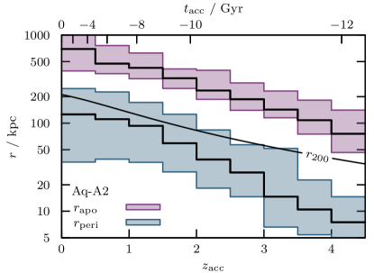
Figure 1: Distribution of apocentre $r_{\mathrm{apo}}$ ( ) and pericentre $r_{\mathrm{peri}}$ ( ) for subhaloes in a Milky Way-like host halo as a function of accretion redshift $z_{\mathrm{acc}}$ (assuming Aquarius cosmological parameters, $H_{0}=73\,\mathrm{km\,s^{-1}}\mathrm{Mpc}^{-1},\Omega_{\mathrm{m}}=0.25,\Omega_{\Lambda}=0.75$). The distribuitions are computed from subhaloes with peak virial masses of $M_{\mathrm{200}}\geq 10^{8}\,\mathrm{M_{\odot}}$ in the Aquarius-A2 simulation. Median radii are shown as solid lines, with shaded regions corresponding to the $16^{\mathrm{th}}-84^{\mathrm{th}}$ percentiles. On average, subhaloes accreted at earlier $z_{\mathrm{acc}}$ have smaller apo- and pericentres than those accreted more recently. Subhaloes with $r_{\mathrm{peri}}<20\,\mathrm{kpc}$ have $z_{\mathrm{acc}}\gtrsim 2$ (i.e., they were accreted $\gtrsim 10\,\mathrm{Gyr}$ ago, see top axis). For reference, the evolution of the host halo virial radius $r_{200}$ is shown as a black solid curve.

2.2 Tidal disruption and numerical resolution

To illustrate the effects of insufficient numerical resolution on tidal evolution, we evolve four different $N$-body realizations of an NFW subhalo in a static isothermal host potential with a circular velocity $V_{\mathrm{host}}=220\,\mathrm{km\,s^{-1}}$ (see Eq. 5). The $N$-body realizations differ only in the number of $N$-body particles used to simulate the subhalo.

2.2.1 Initial conditions

As an example, we consider an NFW subhalo with a virial mass of $M_{200}\approx 7\times 10^{9}\,\mathrm{M_{\odot}}$, close to the redshift $z=0$ hydrogen cooling limit (Benitez-Llambay & Frenk, 2020). For an average concentration of $c=r_{200}/r_{\mathrm{s}}\approx 13$ (Ludlow et al., 2016), this corresponds to an initial a characteristic mass and size of $M_{\mathrm{mx0}}\equiv M(<r_{\mathrm{mx0}})=2\times 10^{9}\,\mathrm{M_{\odot}}$ and $r_{\mathrm{mx0}}=7\,\mathrm{kpc}$, respectively (see Eq. 1 for definition).

Using the code introduced in EP20, available online, we generate four $N$-body realizations of this NFW subhalo: For the first realization, labeled A1, we choose an $N$-body particle mass identical to that used in the Aquarius-A1 simulation, $m_{\mathrm{p}}=1.71\times 10^{3}\,\mathrm{M_{\odot}}$. Similarly, for the second realization, labeled A2, we use $m_{\mathrm{p}}=1.37\times 10^{4}\,\mathrm{M_{\odot}}$, matching the particle mass of the Aquarius-A2 simulation. The models A3 and A4 adopt particle masses that match those of the Aquarius-A3 and A4 resolution levels, respectively. The parameters of these simulations are summarized in Table 1. As the NFW profile has a divergent total mass, we taper the profile exponentially beyond $10\,r_{\mathrm{s}}$ (where by $r_{\mathrm{s}}$ we denote the NFW scale radius as in Eq. 1). Consequently the A1, A2, A3 and A4 realizations of our example subhalo consist of $N=4.4\times 10^{6}$, $5.6\times 10^{5}$, $1.5\times 10^{5}$ and $1.9\times 10^{4}$ particles, respectively.

Table 1: Parameters of the example subhalo model considered in the $N$-body experiments of Sec. 2 and the empirical models of Sec. 3. The initial subhalo mass $M_{\mathrm{mx0}}$ is chosen to approximately match the (redshift $z=0$) hydrogen cooling limit (Benítez-Llambay et al., 2019), and the initial subhalo characteristic size $r_{\mathrm{mx0}}$ is that of a $z=0$ average-concentration halo (Ludlow et al., 2016). Listed also are the host halo and orbit properties underlying the $N$-body and empirical models.

S u b h a l o	Profile	NFW (Eq. 1)
	$M_{\mathrm{mx0}}$, $V_{\mathrm{mx0}}$, $r_{\mathrm{mx0}}$	$2\times 10^{9}\,\mathrm{M_{\odot}}$, $35\,\mathrm{km\,s^{-1}}$, $7\,\mathrm{kpc}$
	$N$-body $\Delta x$	$r_{\mathrm{mx0}}/256\approx 27\,\mathrm{pc}$
	$N$-body $m_{\mathrm{p}}$	A1: $1.71\times 10^{3}\,\mathrm{M_{\odot}}$
		A2: $1.37\times 10^{4}\,\mathrm{M_{\odot}}$
		A3: $4.91\times 10^{4}\,\mathrm{M_{\odot}}$
		A4: $3.93\times 10^{5}\,\mathrm{M_{\odot}}$
H o s t	Profile	Isothermal (Eq. 5)
	$V_{\mathrm{host}}$	$220\,\mathrm{km\,s^{-1}}$
	$r_{\mathrm{peri}}$	$10\,\mathrm{kpc}$
	$r_{\mathrm{peri}}{\,:\,}r_{\mathrm{apo}}$	$1{\,:\,}5$

2.2.2 Simulation code

The simulations are carried out using the particle-mesh code Superbox (Fellhauer et al., 2000). The code employs a high-resolution cubic grid co-moving with the subhalo, with a cell size of $\Delta x\approx r_{\mathrm{mx0}}/256\approx 27\,\mathrm{pc}$. Superbox uses two additional grids, one co-moving of medium resolution ($10\,r_{\mathrm{mx0}}/256$), and a fixed low-resolution ($500\,\mathrm{kpc}/256$) grid containing the entire simulation box. For reference, the force softening length of the Aquarius-A1 simulations equals $\epsilon=22\,\mathrm{pc}$ (Springel et al., 2008), similar to the particle-mesh cell size $\Delta x\approx 27\,\mathrm{pc}$ of the highest-resolving grid used in our numerical experiments. Note that the only parameter varied in the simulations discussed in this section is the $N$-body particle mass $m_{\mathrm{p}}$, and thereby the total number of $N$-body particles in each simulation.

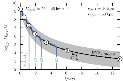
Figure 2: Tidal stripping of a subhalo with an initial mass of $M_{\mathrm{mx0}}=2\times 10^{9}\,\mathrm{M_{\odot}}$ in a Milky Way-like host (see Table 1), computed using N-body simulations (blue curves) and the empirical EN21 model (black solid curve). The four $N$-body simulations have particle masses $m_{\mathrm{p}}$ chosen to match those of the Aquarius-A1 ( ), A2 ( ), A3 ( ) and A4 ( ) resolution levels, respectively. The evolution of the subhalo mass $M_{\mathrm{mx}}$ is shown as a function of time $t$. Numbered circles $⓪,\,...\,,⑥$ mark remnant masses of $\log_{10}M_{\mathrm{mx}}/M_{\mathrm{mx0}}=0,\,-1,\,...\,,\,-6$. Shaded regions correspond to initial conditions spanning a range of circular velocities $20\leq V_{\mathrm{mx0}}/\mathrm{km\,s^{-1}}\leq 40$. Insufficient numerical resolution causes the $N$-body models disrupt artificially, whereas the empirical model predicts an evolution towards a stable asymptotic remnant state.

2.2.3 Simulation results

The NFW subhalo models are placed on an orbit with peri- and apocentric distance $r_{\mathrm{peri}}=10\,\mathrm{kpc}$ and $r_{\mathrm{apo}}=50\,\mathrm{kpc}$, respectively, and evolved for $13\,\mathrm{Gyr}$. Figure 2 shows the evolution of $M_{\mathrm{mx}}$, the bound mass within the radius, $r_{\mathrm{mx}}$, where the circular velocity peaks, as a function of time for the four $N$-body realizations in different shades of blue. As tides strip a subhalo, its mass decreases. Over the first two decades in mass loss, all four $N$-body realizations show a similar evolution. Beyond that point, however, the evolutions diverge. The A4 model fully disrupts after only $\sim 1\,\mathrm{Gyr}$; the A2 model after $\sim 2.5\,\mathrm{Gyr}$. The A1 model survives slightly longer, but eventually also disrupts after a total of $\sim 3.5\,\mathrm{Gyr}$ of evolution.

The increase in $N$-body particle number has hence delayed, but not prevented, the full disruption of the subhalo. This numerical experiment suggests that even simulations with resolution as high as that of the Aquarius-A1 simulation will suffer from the artificial depletion of substructures accreted on orbits that reach the innermost regions of the Galaxy. Even before the subhalo is (artificially) disrupted, its structural evolution is compromised by insufficient resolution: the convergence study listed in appendix A of EN21 shows that once the number of bound particles within $r_{\mathrm{mx}}$ drops below $N_{\mathrm{mx}}<3000$, resolution artifacts result in subhalo densities being systematically underestimated. Evidently, a tool different from classical cosmological $N$-body simulations is needed to model the tidal remnants of heavily stripped dwarf galaxies.

To address this issue, we use in this work an empirical model for the tidal evolution of subhaloes (and embedded dwarf galaxies) which allows us to study their tidal evolution over many orders of magnitude in mass loss. A black solid curve in Figure 2 shows the evolution of the subhalo computed using the empirical EN21 model, available online³. The model suggest that mass loss keeps decelerating, and that a stable remnant state is asymptotically approached. The details of this model, as well as its extension to model the evolution of dwarf galaxies, are summarized in the next chapter.

3 Tidal evolution model

We summarize now the empirical model for tidal stripping used in this work.

3.1 Evolution of the dark matter component

For the evolution of the dark matter component, we rely on the empirical model introduced and tested in EN21. In the initial conditions, the subhalo is assumed to follow an NFW density profile with a scale radius $r_{\mathrm{s}}$ and a scale density $\rho_{\mathrm{s}}$,

$$\rho_{\mathrm{NFW}}(r)=\rho_{\mathrm{s}}\left(r/r_{\mathrm{s}}\right)^{-1}\left(1+r/r_{\mathrm{s}}\right)^{-2}~{}.$$ (1)

Instead of referring to $r_{\mathrm{s}}$ and $\rho_{\mathrm{s}}$ directly, we characterise the subhalo using two equivalent parameters: the peak velocity $V_{\mathrm{mx}}\approx 1.65\,r_{s}\sqrt{G\rho_{s}}$ of the subhalo circular velocity profile $V_{\mathrm{c}}=\sqrt{GM(<r)/r}$, and the radius $r_{\mathrm{mx}}\approx 2.16\,r_{s}$ where the peak velocity is reached. The effect of tides on the subhalo is modelled as an exponential truncation and a re-normalization of the density profile (see EN21 equation 7),

$$\rho(r)=\rho_{\mathrm{NFW}}(r)~{}\times~{}\exp(-r/r_{\mathrm{cut}})/(1+r_{\mathrm{s}}/r_{\mathrm{cut}})^{\kappa}$$ (2)

with $\kappa\approx 0.3$ obtained from fits to $N$-body simulations. For $r_{\mathrm{cut}}/r_{\mathrm{s}}\rightarrow\infty$ the above equation reduces to the initial NFW profile, whereas for strong tidal truncation, $r_{\mathrm{cut}}/r_{\mathrm{s}}\rightarrow 0$, the profile converges to an exponentially truncated cusp,

$$\rho_{\mathrm{asy}}(r)=\rho_{\mathrm{cut}}\exp(-r/r_{\mathrm{cut}})(r/r_{\mathrm{cut}})^{-1}~{}.$$ (3)

For the exponentially truncated cusp, $r_{\mathrm{mx}}\approx 1.79\,r_{\mathrm{cut}}$, $V_{\mathrm{mx}}\approx 1.93\,r_{\mathrm{cut}}\sqrt{G\rho_{\mathrm{cut}}}$. The truncated cusp has a total mass of $M_{\mathrm{cut}}=4\pi\rho_{\mathrm{cut}}r_{\mathrm{cut}}^{3}$, roughly twice as large as the mass $M_{\mathrm{mx}}\approx 0.54\,M_{\mathrm{cut}}$ enclosed within $r_{\mathrm{mx}}$. As tides strip the subhalo, its characteristic velocity $V_{\mathrm{mx}}$ and size $r_{\mathrm{mx}}$ decrease, following a tidal track (see Peñarrubia et al. 2008) that couples the evolution of $V_{\mathrm{mx}}$ to that of $r_{\mathrm{mx}}$ relative to their initial values (here we use the track of EN21; see their equation 5):

$$V_{\mathrm{mx}}/V_{\mathrm{mx0}}=2^{\alpha}(r_{\mathrm{mx}}/r_{\mathrm{mx0}})^{\beta}[1+(r_{\mathrm{mx}}/r_{\mathrm{mx0}})^{2}]^{-\alpha}$$ (4)

with $\alpha\approx 0.4$ and $\beta\approx 0.65$ obtained from fits to $N$-body simulations.

We also use the EN21 model to estimate the time it takes for a subhalo to be stripped to a given remnant mass, assuming that the subhalo is on an orbit with a constant pericentre $r_{\mathrm{peri}}$ and apocentre $r_{\mathrm{apo}}$ within an isothermal host potential,

$$\Phi_{\mathrm{host}}=V_{\mathrm{host}}^{2}~{}\ln\left(r/r_{0}\right)~{},$$ (5)

where by $V_{\mathrm{host}}$ we denote the host’s constant circular velocity, and $r_{0}$ is an arbitrary scale radius.

The rate of tidal stripping depends on the density contrast between subhalo and host, measured at pericentre (EN21 equations 12 and 15). For a given pericentre, the only effect of orbital eccentricity is to delay tidal evolution with respect to the evolution on a circular orbit. For subhaloes that are under-dense with respect to the mean host density at pericentre, tidal evolution gradually decelerates until a final remnant state is reached where the subhalo mean density within $r_{\mathrm{mx}}$ is $\approx 16$ times higher than the mean host density at pericentre. In terms of time scales, heavily stripped subhaloes converge towards a characteristic circular time $T_{\mathrm{mx}}=2\pi r_{\mathrm{mx}}/V_{\mathrm{mx}}\approx T_{\mathrm{peri}}/4$ set by the circular time of the host at pericentre $T_{\mathrm{peri}}=2\pi r_{\mathrm{peri}}/V_{\mathrm{host}}$.

As an example, we use the empirical method outlined here to model the tidal evolution of a dark matter subhalo with the same characteristic mass and size as in the $N$-body example of Sec. 2.2.3 (see Tab. 1), and place it on the same orbit. The time evolution of the dark matter subhalo is shown in Fig. 2: for the range of remnant masses resolved in the $N$-body simulations, there is excellent agreement between the empirical model and the simulation results. During $\sim 13\,\mathrm{Gyr}$ of evolution, the subhalo is stripped to a remnant mass $\sim 10^{6}$ times smaller than its initial mass.

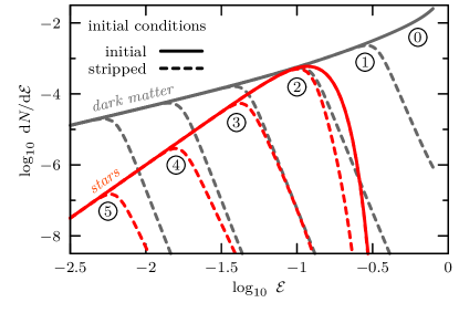
Figure 3: Solid curves show the initial energy distribution $\mathrm{d}N/\mathrm{d}\mathcal{E}$ of dark matter (grey ) and stars (red ), corresponding to snapshot $⓪$ shown in Fig. 4. Dashed curves show the tidally truncated energy distributions of dark matter ( ) and stars ( ) in the initial conditions for remnant subhalo masses of $\log_{10}M_{\mathrm{mx}}/M_{\mathrm{mx0}}=0,\,-1,\,...\,,\,-5$ (snapshots $①,\,...\,,⑤$ ).

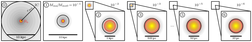
Figure 4: Tidal evolution of a dwarf galaxy embedded in a dark matter subhalo, computed using the empirical energy-truncation model of E+22. The dark matter surface-density $\rho_{\mathrm{2D}}$ is shown in grey, and the surface-brightness $\Sigma_{\star}$ of the embedded dwarf is shown in colour. Snapshots, labeled $⓪,\,...\,,⑥$, are shown for fixed subhalo remnant masses of $\log_{10}M_{\mathrm{mx}}/M_{\mathrm{mx0}}=0,\,-1,\,...\,,\,-6$. The scale is kept constant between the first two panels and the smaller top-left panels. Initially, the stellar component is hardly affected by tides, and mainly dark matter is lost (first three panels). Once the tidal energy truncation reaches the stellar component, the characteristic size of the dark matter halo $r_{\mathrm{mx}}$ (shown as black circles) and the stellar half-light radius $R_{\mathrm{h}}$ (red circles) evolve in parallel (last three panels).

3.2 Evolution of stellar tracers

We now turn our attention to modelling the effect of tides on a stellar system embedded within a dark matter subhalo. We use the model outlined and tested in E+22, where stars are assumed to be massless and collisionless tracers within the subhalo potential. The effect of tides on a dwarf galaxy can then be described through subsequent truncations in the energy distributions of dark matter and stars.

Under the assumptions of spherical symmetry and an isotropic velocity dispersion, for a given subhalo potential, the initial stellar component is fully defined by its initial energy distribution $\mathrm{d}N_{\star}/\mathrm{d}\mathcal{E}$. We parameterize this energy distribution as follows (E+22 equation 13):

$$\mathrm{d}N_{\star}/\mathrm{d}\mathcal{E}=\begin{cases}\mathcal{E}^{\alpha_{\star}}~{}\exp\left[-(\mathcal{E}/\mathcal{E}_{\mathrm{s}})^{\beta_{\star}}\right]&\text{if}~{}0\leq\mathcal{E}<1\\ 0&\text{otherwise.}\end{cases}$$ (6)

In the above equation, binding energies $\mathcal{E}=1-E/\Phi_{0}$ are measured relative to the potential minimum $\Phi_{0}$. In this notation, the most-bound energy state (the ground state) is $\mathcal{E}=0$, and the boundary between bound and unbound particles lies at $\mathcal{E}=1$.

The stellar energy distribution of Equation 6 has a power-law tail towards the most-bound states ($\mathcal{E}\rightarrow 0$) and is exponentially truncated beyond the scale energy $\mathcal{E}_{\mathrm{s}}$. The parameter $\alpha_{\star}$ determines the power-law slope towards the most-bound states, whereas $\beta_{\star}$ modulates the truncation strength for energies beyond $\mathcal{E}_{\mathrm{s}}$. The energy distribution peaks at $\mathcal{E}_{\star}=\mathcal{E}_{\mathrm{s}}~{}\left(\alpha_{\star}/\beta_{\star}\right)^{1/\beta_{\star}}<1$. Figure 3 shows the initial stellar energy distribution for $\alpha_{\star}=3,\beta_{\star}=3$ and a peak energy $\mathcal{E}_{\star}\approx 0.1$ (red solid curve).

Tides truncate this initial stellar energy distribution. We model the truncation empirically through (E+22 eq. 9),

$$\left.\mathrm{d}N_{\star}/\mathrm{d}\mathcal{E}\right|_{\mathrm{i,t}}=\frac{\left.\mathrm{d}N_{\star}/\mathrm{d}\mathcal{E}\right|_{\mathrm{i}}}{1+\left(a\mathcal{E}/\mathcal{E}_{\mathrm{mx,t}}\right)^{b}}$$ (7)

where by $\left.\mathrm{d}N_{\star}/\mathrm{d}\mathcal{E}\right|_{\mathrm{i,t}}$ we denote the truncated energy distribution in the initial conditions, and $\mathcal{E}_{\mathrm{mx,t}}$ is the energy scale beyond which the energy distribution is truncated.

The parameters $a\approx 0.85$, $b\approx 12$ are obtained through fits to $N$-body simulations. This truncated energy distribution is initially out of equilibrium. We model the return to virial equilibrium empirically using fits to $N$-body simulations. The virialization process preserves (on average) the order of energies: the most-bound particles prior to virialization are also (on average) the most-bound particles after virialization. The average mapping of initial pre-virialization energies $\mathcal{E}$ to final energies after virialization follows the empirical relation (E+22 eq. 12)

$$\bar{\mathcal{E}}_{\mathrm{f}}=\left[1+\left(c\mathcal{E}/\mathcal{E}_{\mathrm{mx,t}}\right)^{d}\right]^{1/d}$$ (8)

with $c\approx 0.8$ and $d\approx-3$.

Note that the pre-virialization energies $\mathcal{E}$ are defined in the initial NFW potential, whereas the energies after virialization are defined in the tidally stripped subhalo potential. Under the assumption of isotropic velocity dispersion and spherical symmetry, we then reconstruct the distribution function from the virialized energy distribution,

$$f(\mathcal{E}_{\mathrm{f}})=\mathrm{d}N_{\star}/\mathrm{d}\mathcal{E}_{\mathrm{f}}~{}~{}p^{-1}(\mathcal{E}_{\mathrm{f}})~{},$$ (9)

where $p(\mathcal{E}_{\mathrm{f}})$ is the phase-space volume accessible to a particle with energy $\mathcal{E}_{\mathrm{f}}$ in the stripped subhalo potential. All observable properties of the stellar component can be derived from this distribution function.

The simple empirical method outlined here allows us to model the tidal evolution of accreted substructures down to tiny remnant masses and sizes. In Figure 4, we apply the empirical tidal stripping model to follow the evolution of a dwarf galaxy with an initial projected half-light radius $R_{\mathrm{h}}\approx 440\,\mathrm{pc}$ and an initial luminosity of $L\approx 10^{6}\,\mathrm{L_{\odot}}$. We embed the dwarf galaxy in a subhalo with the same characteristic mass and size as in the $N$-body example of Sec. 2.2.3 (see Tab. 1), and place it on the same orbit.

After $\sim 6\,\mathrm{Gyr}$ of tidal evolution, snapshot ⑤, the dwarf galaxy has been stripped to the size of a micro galaxy, with an enclosed dark matter mass of $\sim 10^{4}\,\mathrm{M_{\odot}}$, a luminosity of only $\sim 10\,\mathrm{L_{\odot}}$ and a size of several tens of parsecs, well beyond the resolution limits of $N$-body simulations like Aquarius-A1 (see Figure 2). After $\sim 12\,\mathrm{Gyr}$ of evolution, snapshot ⑥, the stellar system has been stripped to sub-solar luminosity, but still encloses $\sim 10^{3}\,\mathrm{M_{\odot}}$ of dark matter.

3.3 Dependence of results on the initial stellar density profile

Tidally stripped dwarf galaxies retain some memory of the properties of their initial stellar distribution (E+22). In the following, we will explore how different initial stellar distributions affect the evolution of the remnant luminosity $L$, projected half-light radius $R_{\mathrm{h}}$ and line-of-sight velocity dispersion $\sigma_{\mathrm{los}}$.

3.3.1 Cuspy and cored initial stellar profiles

We will focus on two example initial stellar profiles. The first stellar profile is cored, i.e., $\mathrm{d}\ln\rho_{\star}/\mathrm{d}\ln r\rightarrow 0$ for $r\rightarrow 0$. Its initial energy distribution drops off very steeply towards the most-bound energy states and is given by Equation 6 with $\{\alpha_{\star},\beta_{\star}\}=\{3,3\}$. It is shown as a red solid curve in the example of Fig. 6. The second initial stellar profile follow is cuspy, $\mathrm{d}\ln\rho_{\star}/\mathrm{d}\ln r\rightarrow-1$ for $r\rightarrow 0$, and its energy distribution traces that of the dark matter towards the most-bound energy states: $\{\alpha_{\star},\beta_{\star}\}=\{1,3\}$ in Equation 6.

These two energy distributions are shown in the top panels of Figure 5 for an initial projected half-light radius of $R_{\mathrm{h}}/r_{\mathrm{mx0}}=1/16\approx 440\,\mathrm{pc}$. The corresponding surface brightness $\Sigma_{\star}$ and line-of-sight velocity dispersion $\sigma_{\mathrm{los}}$ profiles are shown in the middle and bottom panel of Figure 5, respectively. The surface brightness profile is normalized to a total luminosity of $L=10^{6}\,\mathrm{L_{\odot}}$, and the velocity dispersion profile assumes an underlying NFW halo with properties as in the example of Table 1. For comparison, using a grey dotted curve, we also show the surface brightness profile obtained by projecting an exponential stellar sphere (Eq. 12) with the same half-light radius $R_{\mathrm{h}}$ and total luminosity $L$.

The velocity dispersion profile of the cored model is centrally flat, whereas the dispersion drops towards the centre for the cuspy model. The luminosity-averaged line-of-sight velocity dispersion,

$$\langle\sigma_{\mathrm{los}}^{2}\rangle = 2\pi\int_{0}^{\infty}\Sigma_{\star}(R)\sigma_{\mathrm{los}}^{2}(R)R~{}\mathrm{d}R$$ (10)

$$= \frac{4\pi G}{3}\int_{0}^{\infty}r\nu_{\star}(r)M(<r)~{}\mathrm{d}r~{},$$ (11)

is virtually identical between the two models (see labelled red and magenta curves in the bottom panel of Fig. 5). In the above equation, we denote by $\nu_{\star}(r)$ the (3D) stellar tracer density, normalized so that $1=4\pi\int_{0}^{\infty}r^{2}\nu_{\star}(r)\,\mathrm{d}r$, and $M(<r)$ is the mass enclosed within a radius $r$ sourcing the potential. Eq. 11 follows from the projected virial theorem (see, e.g. Amorisco & Evans, 2012; Errani et al., 2018), and guarantees that $\langle\sigma_{\mathrm{los}}^{2}\rangle$ is independent of anisotropies in the velocity dispersion. Note that a stochastic realization of the luminosity-averaged $\langle\sigma_{\mathrm{los}}^{2}\rangle$ is likely the only kinematic observable accessible for many faint stellar systems.

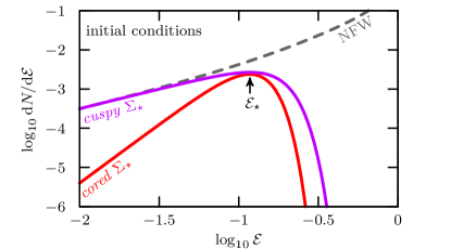
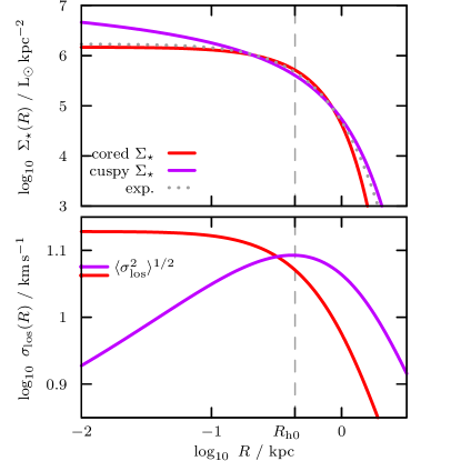
Figure 5: Top panel: Initial energy distribution of a cored ( ) and a cuspy ( ) stellar tracer embedded in an NFW dark matter halo with parameters as in Tab 1. Both models share the same initial projected half-light radius of $R_{\mathrm{h0}}/r_{\mathrm{mx0}}=1/16$. For comparison, the energy distribution of the underlying NFW halo is shown as a grey dashed curve ( ). Middle panel: Corresponding surface brightness profiles $\Sigma_{\star}(R)$. Bottom panel: Line-of-sight velocity dispersion profiles $\sigma_{\mathrm{los}}(R)$. The values of the luminosity-averaged line-of-sight velocity dispersion (Eq. 10) are indicated by short line segments at the left-hand side of the plot.

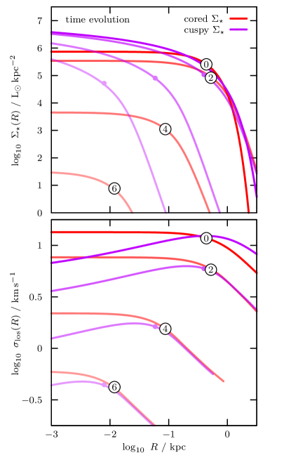
Figure 6: Top panel: Time evolution of the surface brightness profiles of cored ( ) / cuspy ( ) stellar tracers, with initial conditions as shown in Fig. 5. The cored tracer is identical to the model of Fig. 4, with selected snapshots, labeled $⓪,\,...\,,⑥$, shown for fixed subhalo remnant masses of $\log_{10}M_{\mathrm{mx}}/M_{\mathrm{mx0}}=0,\,-2,\,-4\,,\,-6$. The label location coincides with the projected half-light radius. For the cuspy model, the half-light radius is marked using a filled circle. The surface brightness profile of the cored tracer drops much faster than that of its cuspy counterpart. Bottom panel: Time evolution of the corresponding line-of-sight velocity dispersion profiles. Note that in the tidally limited regime, the velocity dispersion profile drops steeply beyond $R_{\mathrm{h}}$.

3.3.2 Time evolution

As tides strip a dwarf galaxy, its surface brightness- and velocity dispersion profile evolve. For a given subhalo and orbit, this evolution depends on the shape of the initial stellar density profile, and on how deeply embedded the stellar profile is within its surrounding dark matter subhalo.

The top panel of Figure 6 shows the time evolution for the cored/cuspy model with initial conditions as in Fig. 5. Profiles are shown for subhalo remnant masses of $\log_{10}M_{\mathrm{mx}}/M_{\mathrm{mx0}}=0,\,-2,\,-4\,,\,-6$. In the early stages of tidal evolution, the surface brightness profile is hardly affected by tides. Once the example subhalo has lost $\sim 99$ per cent of its initial characteristic mass, the tidal energy truncation reaches the stellar component (snapshot ②, compare Fig. 3). From that point on, the surface brightness of the stellar component decreases with each further tidal energy truncation, and the half-light radius of the stellar component decreases.

For the cored stellar model (red curves), this evolution is illustrated also in Fig. 4. The surface brightness of the stellar component is shown in colour, whereas the dark matter surface density is shown in grey. After a slight initial expansion of the stellar half-light radius $R_{\mathrm{h}}$ (shown as a red circle), once the tidal energy truncation has reached the stellar component, dark matter and stars are truncated approximately beyond the same radius, and the stellar half-light radius $R_{\mathrm{h}}$ evolves in sync (Kravtsov, 2010) with the characteristic size $r_{\mathrm{mx}}$ (black circle) of the underlying dark matter subhalo.

Returning to Fig. 6, we see that the surface brightness of the cored stellar tracer (red curves) drops much more rapidly during tidal stripping than the surface brightness of its cuspy counterpart (magenta curves). This disparate evolution is easily understood when looking at the underlying stellar energy distributions (Fig. 5).

As tides truncate the dwarf galaxy in energy, the cuspy model loses stars and dark matter at a similar pace, as its stellar energy distribution follows that of the dark matter towards the most-bound energy states. The cored stellar model instead hardly populates the most-bound energy states: its stellar energy distribution drops much more rapidly towards the most-bound states than that of the dark matter. The prospect of observing micro galaxies hence hinges crucially on how stars are distributed within the dark matter subhalo energetically.

The bottom panel of Fig. 6 shows the time evolution of the corresponding line-of-sight velocity dispersion profiles. The mean velocity dispersion of both the cored and the cuspy tracer drops monotonously with tidal mass loss.

4 Application to Local Group satellites

We are now ready to apply the model outlined in Section 3 to predict the luminosity, structure and kinematics of heavily-stripped micro galaxies. We compare these predicted properties against those of observed stellar systems in the Local Group. In particular, we aim to address the nature of recently discovered stellar systems at the boundary between the globular cluster and dwarf galaxy regime, with half-light radii $1\lesssim R_{\mathrm{h}}/\mathrm{pc}\lesssim 30$ and luminosities of $10\lesssim L/\mathrm{L_{\odot}}\lesssim 10^{3}$ (Torrealba et al., 2019; Mau et al., 2020; Cerny et al., 2022, 2023; Smith et al., 2023). If these systems are gravitationally bound, then, in principle, they could be one of three possibilities: (1) self-gravitating star clusters devoid of dark matter, like globular clusters; (2) dark-matter dominated galaxies whose sizes and luminosities have not changed dramatically since formation; or (3) dark matter-dominated micro galaxies of tidal origin, formed through stripping of larger and more luminous progenitors.

4.1 Half-light radii and luminosities

Figure 7a shows a compilation of projected half-light radii $R_{\mathrm{h}}$ of Local Group dwarf galaxies (blue circles) and globular clusters (yellow triangles). On average, at equal luminosity, globular clusters are significantly more compact than dwarf galaxies. For example, at $L=10^{6}\,\mathrm{L_{\odot}}$, globular clusters span a range in sizes of roughly $1\sim 10\,\mathrm{pc}$, more than an order of magnitude more compact than dwarfs of the same luminosity, $0.1\sim 1\,\mathrm{kpc}$. This clear separation in size becomes ambiguous at lower luminosities. Ultra-faint dwarfs like the Tucana 3 and Draco 2 dSphs with luminosities of $10^{3}\sim 10^{4}\,\mathrm{L_{\odot}}$ have half-light radii of $20\sim 50\,\mathrm{pc}$, not too different from extended Milky Way globular clusters like Palomar 5 or Palomar 14. This ambiguity persists at lower luminosities: The recently discovered objects, labelled “unidentified” and depicted as grey crosses in Fig. 7a, populate a parameter space at the boundary between the globular cluster- and dwarf galaxy regimes.

To address whether these ambiguous objects could be the remnants of tidally stripped dwarf galaxies, we show the evolution of two dwarf galaxy models in Fig. 7a, computed using the method outlined in Sec. 3. The evolution of size and luminosity for a dwarf galaxy with a cored surface brightness profile is shown in red, for an initial luminosity of $L_{0}=10^{6}\,\mathrm{L_{\odot}}$ and an initial half-light radius of $R_{\mathrm{h0}}=440\,\mathrm{pc}$ (identical to the model shown in Fig. 3 and 4, with circled numbers $⓪,\,...\,,⑥$ corresponding to fixed subhalo remnant masses of $\log_{10}M_{\mathrm{mx}}/M_{\mathrm{mx0}}=0,\,-1,\,...\,,\,-6$).

As tides remove stars from the cored model, its size and luminosity drop. The evolution moves the dwarf galaxy model away from the observed mass-size relation of dwarf galaxies, and, for the choice of initial conditions made here, the stripped system does not reach the parameter space occupied by the recently-discovered objects at the boundary between the globular cluster and dwarf galaxy regimes.

As discussed in Section 3.3, the evolution of size and luminosity crucially depends on the shape of the initial stellar density profile, which in turn depends on the degree to which stellar binding energies extend to the most-bound energy states in the subhalo. The evolution of a stellar tracer with a cuspy surface brightness profile (total luminosity and half-light radius identical to the cored model discussed previously) is shown as a magenta curve in Fig. 7a. For this cuspy model, the drop in luminosity is less steep: tidal evolution shifts the dwarf galaxy model roughly along the observed mass-size relation of dwarf galaxies, and, for the example initial conditions chosen here, the stripped model approaches the parameter space that bridges the globular cluster and dwarf galaxy regimes.

We conclude that measurements of size and luminosity alone are not sufficient to decide whether a stellar system at the interface of the globular cluster and dwarf galaxy regimes may be the remnant of a tidally stripped dwarf galaxy. Clearer observational evidence and/or theoretical understanding is needed to constrain the initial stellar energy distribution, and thereby the tidal fate of heavily-stripped dwarf galaxies in the size/luminosity plane.

Figure 7: (a) Luminosities $L$ and half-light radii $R_{\mathrm{h}}$ of Local Group dwarf galaxies ( ) and globular clusters ( ). Objects at the boundary between the dwarf- and globular cluster regime are marked using grey crosses ( ). For references, see footnote 5. Tidal tracks for the evolution of a cored ( ) and a cuspy ( ) stellar tracer (as in Fig. 5) are shown in purple and red, respectively. Snapshots, labeled $⓪,\,...\,,⑥$, are highlighted for fixed subhalo remnant masses of $\log_{10}M_{\mathrm{mx}}/M_{\mathrm{mx0}}=0,\,-1,\,...\,,\,-6$. The luminosity of a cored stellar tracer drops more rapidly during tidal stripping than that of its cuspy counterpart. (b) Line-of-sight velocity dispersion $\langle\sigma_{\mathrm{los}}^{2}\rangle^{1/2}$ (Eq. 10) and projected half-light radius $R_{\mathrm{h}}$. The top black curve labelled “initial” shows the line-of-sight velocity dispersion expected for a stellar tracer of half-light radius $R_{\mathrm{h}}$ embedded in a $\sim 10^{9}\,\mathrm{M_{\odot}}$ dark matter halo, while the bottom curve corresponds to a halo that has been stripped to $10^{-6}$ of its initial mass. Yellow crosses ( ) show velocity dispersions computed under the assumption of self-gravity. (c) Luminosities $L$ and dynamical masses $M_{\mathrm{1.8}}$ (Eq. 15). Diagonal lines mark constant dynamical mass-to-light ratios of $M_{1.8}/L=1\,\mathrm{M_{\odot}}/\mathrm{L_{\odot}}$ and $100\,\mathrm{M_{\odot}}/\mathrm{L_{\odot}}$. While the mass-to-light ratio of the cored stellar model increases during tidal evolution, for the model with cuspy surface brightness profile, the mass-to-light ratio converges to a constant. (d) Projected half-light radii $R_{\mathrm{h}}$ and mean densities $\bar{\rho}_{1.8}$ (Eq. 16) enclosed within a spherical radius of $1.8\,R_{\mathrm{h}}$.

4.2 Half-light radii and velocity dispersions

As discussed in the previous section, size and luminosity alone are not sufficient to tell whether an observed stellar system is self-gravitating, akin to a globular cluster, or dark matter dominated, like dwarf galaxies and their remnants. We now discuss to what extent measurements of the line-of-sight velocity dispersion $\langle\sigma_{\mathrm{los}}^{2}\rangle^{1/2}$ (Eq. 10) can help to constrain the possible progenitors of observed stellar systems. Fig. 7b shows the half-light radii $R_{\mathrm{h}}$ and line-of-sight velocity dispersions $\langle\sigma_{\mathrm{los}}^{2}\rangle^{1/2}$ for the same dwarf galaxies and globular clusters as in Fig. 7a. Dwarf galaxies, on average, are more extended than globular clusters at equal velocity dispersion.

4.2.1 Self-gravitating star clusters

For most of the objects marked as “unidentified” in Fig. 7a, no robust measure of velocity dispersion is available to date. If these objects were self-gravitating and devoid of dark matter, their velocity dispersion could be estimated from their half-light radius $R_{\mathrm{h}}$ and their total stellar mass $M_{\star}$. Assuming an exponential density profile for the stellar tracer,

$$\rho_{\star}(r)=M_{\star}/(8\pi r_{\star}^{3})~{}\exp(-r/r_{\star})$$ (12)

with $R_{\mathrm{h}}\approx 2.02\,r_{\star}$ and total stellar mass $M_{\star}$, Eq. 11 gives

$$\langle\sigma_{\mathrm{los}}^{2}\rangle=(5/96)~{}GM_{\star}/r_{\star}~{}.$$ (13)

For each “unidentified” system shown in Fig. 7a, we use Eq. 13 to estimate the (virial) velocity dispersion the object would have if it was fully self-gravitating. For this calculation, we assume a mean stellar mass-to-light ratio of $\Upsilon\approx 1.6$ (Woo et al., 2008). The results of this exercise are marked as yellow crosses in Fig. 7b. For reference, dashed diagonal lines in Fig. 7b are also computed from Eq. 13, for constant stellar masses of $M_{\star}=\Upsilon L=10^{2}$, $10^{3}$ and $10^{4}\,\mathrm{M_{\odot}}$.

4.2.2 Dark matter-dominated objects

Dwarf galaxies, with their velocity dispersion predominantly supported by the dark matter component, generally exhibit much larger velocity dispersions than possible by self-gravity of their stellar components alone. To estimate the contribution to the velocity dispersion of the dark matter component, we make use of the notion that within the LCDM framework, dwarf galaxies are expected to form within a relatively narrow range of halo masses.

The lower limit on this halo mass is set by the constraint that gas must be able cool in presence of the cosmic UV background: only haloes with masses above the hydrogen cooling limit provide the necessary conditions for the onset of star formation. At redshift $z=0$, the limiting virial mass equals roughly $\sim 5\times 10^{9}\,\mathrm{M_{\odot}}$ (see, e.g., Benitez-Llambay & Frenk, 2020). The velocity dispersion of an exponential stellar profile embedded in an average-concentration NFW halo with a halo mass close to the $z=0$ hydrogen cooling limit ($r_{\mathrm{mx0}}=7\,\mathrm{kpc}$, $V_{\mathrm{mx0}}=35\,\mathrm{km\,s^{-1}}$, see Table 1) is shown as a black solid curve in Fig. 7b, labelled “initial”. This curve is computed from Eq. 11, with the integral evaluated numerically.

More generally, cosmological simulations suggest that satellite dwarf galaxies of Milky Way-like host galaxies formed within dark matter haloes of peak circular velocity $20\lesssim V_{\mathrm{mx}}/\mathrm{km\,s^{-1}}\lesssim 40$ (Fattahi et al., 2018). This range of potential initial haloes is indicated by the grey band in Fig. 7b, which includes $\pm 0.1\,\mathrm{dex}$ variation in concentration around the mean. Note that many dSphs of the Local Group fall within this band, suggesting that they have experienced only minor tidal perturbation.

The current-day sizes and dispersions of dwarf galaxies and their remnants do depend on their properties at formation, and their tidal history. Dwarf galaxies that experienced little tidal mass loss would be located within the grey band of Fig. 7b. Tides allow dwarf galaxies to drop to velocity dispersions below the grey band. To illustrate the underlying systematics, we show the tidal evolution of half-light radius $R_{\mathrm{h}}$ and velocity dispersion $\langle\sigma_{\mathrm{los}}^{2}\rangle^{1/2}$ of two example dwarf galaxy models with cored and cuspy stellar tracers using red and magenta curves in Fig. 7b. Both models are initially located at the position marked ⓪, and are embedded in the same dark matter halo. As previously, circled numbers $⓪,\,...\,,\,,⑥$ correspond to the snapshots shown in Fig. 4 at fixed subhalo remnant masses of $\log_{10}M_{\mathrm{mx}}/M_{\mathrm{mx0}}=0,\,-1,\,...\,,\,-6$.

In the early stages of tidal evolution, the tidal energy truncation does not reach the binding energies of the stars (compare Fig. 3). Dark matter on less-bound orbits is removed by tides. Some of these orbits do contribute to the density within the stellar radii: after their removal, the velocity dispersion of an embedded stellar tracer drops. This causes the initial near-vertical evolution in the size-velocity dispersion plane. Once the tidal energy truncation has reached the stellar component (in the example shown, this corresponds roughly to snapshot ②), size and velocity dispersion of stars and dark matter evolve in sync, both decreasing monotonously. This is the regime we refer to as tidally limited in E+22. In this regime, for the cored stellar tracer, we find $R_{\mathrm{h}}/r_{\mathrm{mx}}\approx 0.9$ and $\langle\sigma_{\mathrm{los}}^{2}\rangle^{1/2}/V_{\mathrm{mx}}\approx 0.5$. Similarly, for the cuspy stellar tracer, $R_{\mathrm{h}}/r_{\mathrm{mx}}\approx 0.6$ and $\langle\sigma_{\mathrm{los}}^{2}\rangle^{1/2}/V_{\mathrm{mx}}\approx 0.5$.

The initial shape of the stellar density profile appears to play only a secondary role in the evolution of half-light radius and luminosity-averaged line-of-sight velocity dispersion; the model predictions for cored (red) and cuspy (magenta) stellar tracers in Fig. 7b differ very little.

The bottom curve, passing through the snapshot ⑥, shows the velocity dispersion expected for an exponential stellar tracer embedded in a tidally stripped truncated cusp halo (Eq. 3). This stage of tidal evolution, close to the asymptotic remnant state, is reached after $13\,\mathrm{Gyr}$ on an orbit with $r_{\mathrm{peri}}=10\,\mathrm{kpc}$ (see Fig. 2). Eq. 11 gives

$$\langle\sigma_{\mathrm{los}}^{2}\rangle=\frac{GM_{\mathrm{cut}}}{6\,r_{\mathrm{cut}}}~{}\frac{(r_{\star}/r_{\mathrm{cut}})\left(3+r_{\star}/r_{\mathrm{cut}}\right)}{\left(1+r_{\star}/r_{\mathrm{cut}}\right)^{3}}~{},$$ (14)

where, as before, $r_{\star}\approx R_{\mathrm{h}}/2.02$, and $r_{\mathrm{cut}}\approx r_{\mathrm{mx}}/1.79$. For tidally limited systems, the size of a stellar tracer is constrained to be at most as extended as the surrounding (tidally truncated) dark matter halo. Hence, in Fig. 7b, we plot Eq. 14 only for $R_{\mathrm{h}}\lesssim r_{\mathrm{mx}}$.

We can now return to the objects marked “unidentified” in Fig. 7a. If these objects were dark matter-dominated and only weakly affected by tides, they would have velocity dispersions in the grey-shaded area of Fig. 7b. If instead these objects were subject to strong tides, their velocity dispersions should fall within the region highlighted in blue in Fig. 7b. In either of the two cases, for most of the “unidentified” objects, the predicted dispersions for the dark matter-dominated formation scenario are higher than those expected for self-gravitating objects (yellow crosses).

These results suggest that accurate velocity dispersion estimates of micro galaxy candidates can help to distinguish them from globular cluster remnants. Our model predictions are relatively insensitive to the (unknown) initial energy distribution of stars within the dark matter halo. The required level of measurement accuracy is challenging, with (virial) velocity dispersions in the dark matter-dominated case ranging from several hundred $\mathrm{m}\mathrm{s}^{-1}$ to a few $\mathrm{km\,s^{-1}}$. Accurate multi-epoch spectroscopy will be required to estimate the contribution of binaries to the observed dispersions (see, e.g., McConnachie & Côté, 2010; Koposov et al., 2011; Minor et al., 2019).

4.3 Dynamical mass-to-light ratio

As discussed in the previous section, micro galaxies would differ from globular clusters in their dark matter content. The virial theorem can be used to estimate the dynamical mass enclosed within the luminous radius of a stellar system through the combined measurement of half-light radius $R_{\mathrm{h}}$ and luminosity-averaged velocity dispersion $\langle\sigma_{\mathrm{los}}^{2}\rangle$ (Illingworth, 1976; Merritt, 1987; Amorisco & Evans, 2012). We will in the following adopt the mass estimator derived in Errani et al. (2018), which is insensitive to anisotropies in the velocity dispersion, and minimizes uncertainties introduced by the (unknown) dark matter density profile shape and extent. The estimator yields the mass enclosed within a spherical radius of $\sim 1.8\,R_{\mathrm{h}}$,

$$M_{1.8}\equiv M(<1.8\,R_{\mathrm{h}})\approx 3.5\times 1.8\,R_{\mathrm{h}}~{}\sigma_{\mathrm{los}}^{2}~{}G^{-1}~{}.$$ (15)

In Fig. 7c, we compare the dynamical mass $M_{1.8}$ of Local Group dwarf galaxies and globular clusters against their total luminosity $L$. Globular cluster luminosity and dynamical mass are distributed with little scatter around a line of constant dynamical mass-to-light ratio $M_{1.8}/L\approx 1\,\mathrm{M_{\odot}}/\mathrm{L_{\odot}}$. Dwarf galaxies, on the other hand, span wide range of dynamical mass-to-light ratios, $10\lesssim(M_{1.8}/L)(\mathrm{M_{\odot}}/\mathrm{L_{\odot}})^{-1}\lesssim 10^{4}$.

The tidal evolution of the dynamical mass-to-light ratio crucially depends on the shape of the stellar density profile. The dynamical mass-to-light ratio of the cored model shown in red in Fig. 7c gradually increases in the regime of heavy mass loss, as its stellar energy distribution drops more steeply towards the most-bound states than that of the surrounding dark matter halo (see Fig. 5). As the tidal mass loss progresses, the cored stellar system hence becomes more and more dark matter dominated. In contrast, the mass-to-light ratio of the cuspy stellar model (with a stellar energy distribution which traces that of the dark matter) converges during tidal stripping to a constant value. This asymptotic mass-to-light ratio is lower than the mass-to-light ratio at accretion. Yet, for the examples considered here, the dwarf galaxies do remain dark matter dominated throughout their evolution. Micro galaxies can therefore be distinguished from globular clusters by their dark matter content, either directly, through measurements of their stellar velocity dispersions (see Sec. 4.2), or indirectly, by studying their susceptibility to tidal forces along their orbit (see Errani et al., 2023b).

4.4 Enclosed mean density

Using the enclosed dynamical mass $M_{1.8}$ defined by Eq. 15, we can estimate the density of a stellar system averaged within a spherical radius of $1.8\,R_{\mathrm{h}}$,

$$\bar{\rho}_{1.8}\equiv M_{1.8}~{}(1.8\,R_{\mathrm{h}})^{-3}~{}(4\pi/3)^{-1}~{}.$$ (16)

Fig. 7d shows the enclosed mean densities $\bar{\rho}_{1.8}$ of Milky Way satellites as a function of their half-light radii $R_{\mathrm{h}}$. All elements of Fig. 7d are analogous to Fig. 7b, but expressed in terms of density. This allows for an intuitive description of the tidal evolution of dwarf galaxies. In the early stages of tidal evolution, luminosity and extent of the stellar component are hardly affected. Yet, the mean density enclosed within the luminous radii drops, as dark matter on less-bound orbits is stripped (snapshot $①$). Once the tidal energy truncation affects the stellar component, its size decreases (snapshot $②$). At the same time, its mean density gradually increases: the smaller the remaining stellar system, the higher the average density of the underlying cuspy dark matter halo enclosed within the luminous radii.

Returning to the objects marked as “unidentified” in Fig. 7a, we note that, for most of these objects, their mean densities if self-gravitating (yellow crosses) are substantially lower than the model prediction for dark matter-dominated micro galaxies (blue region). Remarkably, if self-gravitating, the mean densities of several of the ‘unidentified’ systems are comparable to the mean density of the Milky Way at the solar circle, $\bar{\rho}_{\mathrm{MW}}(R_{\odot})\approx 5\times 10^{7}\,\mathrm{M_{\odot}}\,\mathrm{kpc}^{-3}$ (assuming $R_{\odot}=8.3\,\mathrm{kpc}$ and a circular velocity of $240\,\mathrm{km\,s^{-1}}$). This in turn implies that these objects are likely vulnerable to tides, which offers an alternative probe to constrain their potential dark matter content.

4.5 How many?

The model outlined in Sec. 3 enables predictions of the luminosities, sizes and velocity dispersions of heavily-stripped dwarf galaxies – but not their expected abundance in the Milky Way. While the actual number of heavily-stripped satellites in the inner regions of the Milky Way will depend on its detailed mass assembly history, with the aim of developing a rough understanding of the underlying systematics, we will in the following discuss how the subhalo mass function and the minimum halo mass for star formation affect the number of expected micro galaxies.

Cosmological simulations show that in LCDM, the subhalo mass function is relatively steep. For the Aquarius A halo, Springel et al. (2008) measure $\mathrm{d}\ln N_{\mathrm{sub}}/\mathrm{d}\ln M_{\mathrm{sub}}\approx-1.9$, i.e., roughly speaking, the number of subhaloes per log-spaced mass bin is inversely proportional to the subhalo mass.

Not all subhaloes host a galaxy, though. Only haloes above some threshold mass allow hydrogen gas to cool in presence of the cosmic UV background, and in turn, to collapse and form stars (see, e.g. Bullock et al., 2000; Gnedin, 2000). The critical mass model discussed in Benitez-Llambay & Frenk (2020) implies a redshift-dependent minimum halo mass for star formation which, at $z=0$, equals $\sim 5\times 10^{9}\,\mathrm{M_{\odot}}$ (at $z=3$ and $z=5$, the values are $\sim 1\times 10^{9}\,\mathrm{M_{\odot}}$ and $\sim 5\times 10^{8}\,\mathrm{M_{\odot}}$ , respectively). Galaxies which formed their stars prior to reionization may have formed in haloes of even smaller masses: Bovill & Ricotti (2009) suggest a threshold of only $\sim 2\times 10^{8}\,\mathrm{M_{\odot}}$. Within the $z=0$ virial radius of the Aquarius-A2 main halo ($r_{200}\approx 246\,\mathrm{kpc}$) we count $N_{\mathrm{sub}}=16$, $69$, $151$ and $351$ subhaloes with peak masses above $5\times 10^{9}\,\mathrm{M_{\odot}}$, $1\times 10^{9}\,\mathrm{M_{\odot}}$, $5\times 10^{8}\,\mathrm{M_{\odot}}$ and $2\times 10^{8}\,\mathrm{M_{\odot}}$, respectively.

For a numerical example of the number of subhaloes that reach the inner regions of a Milky Way-like halo, we return to study the orbits of subhaloes in the Aquarius-A2 merger tree. As previously, we treat subhaloes as point-masses, and integrate their orbits from their respective redshift of accretion $z_{\mathrm{acc}}$ till $z=0$. We assume a time-evolving, analytical potential fitted to the A2 main halo (see Sec. 2.1 for details). This allows us to follow the evolution of all subhaloes resolved at accretion till $z=0$, without losing subhaloes to artificial disruption. We find that within a galactocentric radius of $r_{200}\approx 246\,\mathrm{kpc}$ there are $33$ subhaloes with peak virial masses $M_{\mathrm{peak}}\geq 1\times 10^{9}\,\mathrm{M_{\odot}}$ on orbits with pericentric distances $r_{\mathrm{peri}}\leq 20\,\mathrm{kpc}$, and $16$ subhaloes have $r_{\mathrm{peri}}\leq 10\,\mathrm{kpc}$. Decreasing the mass threshold to $M_{\mathrm{peak}}\geq 2\times 10^{8}\,\mathrm{M_{\odot}}$ increases the number of subhaloes with $r_{\mathrm{peri}}\leq 20\,\mathrm{kpc}$ to 171, and the number of those with $r_{\mathrm{peri}}\leq 10\,\mathrm{kpc}$ to 92. Note that cosmological variance will introduce a substantial halo-to-halo variance of these numbers, in particular at the higher-mass end (see figure 8 in Springel et al. 2008 comparing the subhalo abundance in the Aquarius A–F main haloes).

The strong dependence of the subhalo abundance on the choice of threshold mass is a direct consequence of the steep underlying subhalo mass function. We conclude that observational constraints on the abundance of micro galaxies would inform us equally about the number of dark matter subhaloes in the inner Milky Way, and about the minimum mass of star-forming subhaloes.

5 Summary and conclusions

In LCDM cosmology, dark matter haloes are predicted to have remarkably dense centres where the density profiles formally diverge as $\mathrm{d}\ln\rho/\mathrm{d}\ln r=-1$ for $r\rightarrow 0$. These density cusps render LCDM subhaloes resilient to the effect of tides, and prevent the full tidal disruption of subhaloes and embedded dwarf galaxies. The hierarchical accretion history of the Milky Way may therefore give rise to a population of heavily stripped “micro galaxies”, i.e., co-moving groups of stars, held together and shielded from Galactic tides by a surrounding dark matter subhalo. The resilience to full tidal disruption contrasts LCDM from other dark matter theories that predict haloes with central constant-density cores, and/or lower mean central densities, such as ultralight-particle DM models, or self-interacting dark matter (SIDM) models (prior to the onset of core-collapse).

In this study, we use an empirical framework to model the evolution of size, luminosity and velocity dispersion of stellar systems embedded in LCDM subhaloes, following their tidal evolution over many orders of magnitude in mass, luminosity, and size. We discuss our findings in the context of recently-discovered faint stellar systems with structural properties at the boundary of the globular cluster- and dwarf galaxy regimes. Our main conclusions are summarized below.

• Current cosmological simulations cannot accurately predict the structure, kinematics and abundance of subhaloes and embedded dwarf galaxies around the solar circle. Insufficient $N$-body particle number and spatial resolution drive the artificial disruption of substructures in the inner regions of simulated Milky Way-like haloes. A route to circumvent such resolution limits are (semi-) analytical models like the one discussed in this work.

• Consistent with earlier work, we show that if a stellar tracer populates the energy states of a CDM halo all the way down to the most-bound state, then smooth tidal fields can never fully disrupt that stellar tracer. This suggests the possible existence of micro galaxies, co-moving stellar systems of low total luminosity, stabilized against Galactic tides by a surrounding dark matter subhalo.

• The evolution of luminosity and size of such objects is very sensitive to the (unknown) initial binding energy distribution of a stellar tracer within its surrounding dark matter halo.

• In contrast, the tidal evolution of half-light radius and velocity dispersion only weakly depends on the initial stellar energy distribution.

• Velocity dispersion measurements provide a robust criterion to distinguish self-gravitating stellar systems from dark matter-dominated micro galaxies. For orbits with pericentres around the solar circle, we predict (virial) velocity dispersions between several hundred $\mathrm{m}\,\mathrm{s}^{-1}$ and a few $\mathrm{km\,s^{-1}}$. Resolving such dispersions for faint stellar systems represents a considerable challenge. Multi-epoch spectroscopy will be required to accurately account for the contribution of binary stars to the observed dispersions.

• Dark matter-dominated micro galaxies have larger mean densities than their self-gravitating counterparts of equal luminosity. For systems where accurate stellar velocities are unavailable, the susceptibility to tides can therefore serve as an alternative criterion to distinguish globular clusters from micro galaxies.

The discovery of dark matter-dominated micro galaxies would inform us about the ability of dark matter subhaloes to survive in the Milky Way tidal field, and at the same time, suggest that stars can populate the most-bound energy states of a halo. Hence, micro galaxies would offer equally insight in the physical properties of dark matter subhaloes, and the baryonic processes that shape the galaxies embedded therein.

Acknowledgements

RE and RI acknowledge funding from the European Research Council (ERC) under the European Unions Horizon 2020 research and innovation programme (grant agreement number 834148). RE and MW acknowledge support from the National Science Foundation (NSF) grants AST-2206046 and AST-1909584.

References

- Amorisco et al. (2013) Amorisco, N. C., Agnello, A., & Evans, N. W. 2013, MNRAS, 429, L89, doi: 10.1093/mnrasl/sls031
- Amorisco & Evans (2012) Amorisco, N. C., & Evans, N. W. 2012, MNRAS, 419, 184, doi: 10.1111/j.1365-2966.2011.19684.x
- Battaglia & Nipoti (2022) Battaglia, G., & Nipoti, C. 2022, Nature Astronomy, 6, 659, doi: 10.1038/s41550-022-01638-7
- Battaglia et al. (2022) Battaglia, G., Taibi, S., Thomas, G. F., & Fritz, T. K. 2022, A&A, 657, A54, doi: 10.1051/0004-6361/202141528
- Baumgardt et al. (2009) Baumgardt, H., Côté, P., Hilker, M., et al. 2009, MNRAS, 396, 2051, doi: 10.1111/j.1365-2966.2009.14932.x
- Benitez-Llambay & Frenk (2020) Benitez-Llambay, A., & Frenk, C. 2020, MNRAS, 498, 4887, doi: 10.1093/mnras/staa2698
- Benítez-Llambay et al. (2019) Benítez-Llambay, A., Frenk, C. S., Ludlow, A. D., & Navarro, J. F. 2019, MNRAS, 488, 2387, doi: 10.1093/mnras/stz1890
- Borukhovetskaya et al. (2022) Borukhovetskaya, A., Navarro, J. F., Errani, R., & Fattahi, A. 2022, MNRAS, 512, 5247, doi: 10.1093/mnras/stac653
- Bovill & Ricotti (2009) Bovill, M. S., & Ricotti, M. 2009, ApJ, 693, 1859, doi: 10.1088/0004-637X/693/2/1859
- Bruce et al. (2023) Bruce, J., Li, T. S., Pace, A. B., et al. 2023, ApJ, 950, 167, doi: 10.3847/1538-4357/acc943
- Buist & Helmi (2016) Buist, H. J. T., & Helmi, A. 2016, A&A, 589, C3, doi: 10.1051/0004-6361/201323059e
- Bullock et al. (2000) Bullock, J. S., Kravtsov, A. V., & Weinberg, D. H. 2000, ApJ, 539, 517, doi: 10.1086/309279
- Burkert (2000) Burkert, A. 2000, ApJ, 534, L143, doi: 10.1086/312674
- Cautun & Frenk (2017) Cautun, M., & Frenk, C. S. 2017, MNRAS, 468, L41, doi: 10.1093/mnrasl/slx025
- Cerny et al. (2022) Cerny, W., Martínez-Vázquez, C. E., Drlica-Wagner, A., et al. 2022, arXiv e-prints, arXiv:2209.12422, doi: 10.48550/arXiv.2209.12422
- Cerny et al. (2023) Cerny, W., Simon, J. D., Li, T. S., et al. 2023, ApJ, 942, 111, doi: 10.3847/1538-4357/aca1c3
- Chiti et al. (2021) Chiti, A., Frebel, A., Simon, J. D., et al. 2021, Nature Astronomy, 5, 392, doi: 10.1038/s41550-020-01285-w
- Colín et al. (2002) Colín, P., Avila-Reese, V., Valenzuela, O., & Firmani, C. 2002, ApJ, 581, 777, doi: 10.1086/344259
- Collins et al. (2020) Collins, M. L. M., Tollerud, E. J., Rich, R. M., et al. 2020, MNRAS, 491, 3496, doi: 10.1093/mnras/stz3252
- Collins et al. (2021) Collins, M. L. M., Read, J. I., Ibata, R. A., et al. 2021, MNRAS, 505, 5686, doi: 10.1093/mnras/stab1624
- Diakogiannis et al. (2017) Diakogiannis, F. I., Lewis, G. F., Ibata, R. A., et al. 2017, MNRAS, 470, 2034, doi: 10.1093/mnras/stx1219
- D’Onghia et al. (2010) D’Onghia, E., Springel, V., Hernquist, L., & Keres, D. 2010, ApJ, 709, 1138, doi: 10.1088/0004-637X/709/2/1138
- Errani & Navarro (2021) Errani, R., & Navarro, J. F. 2021, MNRAS, 505, 18, doi: 10.1093/mnras/stab1215
- Errani et al. (2022) Errani, R., Navarro, J. F., Ibata, R., & Peñarrubia, J. 2022, MNRAS, 511, 6001, doi: 10.1093/mnras/stac476
- Errani et al. (2023a) Errani, R., Navarro, J. F., Peñarrubia, J., Famaey, B., & Ibata, R. 2023a, MNRAS, 519, 384, doi: 10.1093/mnras/stac3499
- Errani et al. (2023b) Errani, R., Navarro, J. F., Smith, S. E. T., & McConnachie, A. W. 2023b, arXiv e-prints, arXiv:2311.10134. https://arxiv.org/abs/2311.10134
- Errani & Peñarrubia (2020) Errani, R., & Peñarrubia, J. 2020, MNRAS, 491, 4591, doi: 10.1093/mnras/stz3349
- Errani et al. (2017) Errani, R., Peñarrubia, J., Laporte, C. F. P., & Gómez, F. A. 2017, MNRAS, 465, L59, doi: 10.1093/mnrasl/slw211
- Errani et al. (2018) Errani, R., Peñarrubia, J., & Walker, M. G. 2018, MNRAS, 481, 5073, doi: 10.1093/mnras/sty2505
- Fattahi et al. (2018) Fattahi, A., Navarro, J. F., Frenk, C. S., et al. 2018, MNRAS, 476, 3816, doi: 10.1093/mnras/sty408
- Fellhauer et al. (2000) Fellhauer, M., Kroupa, P., Baumgardt, H., et al. 2000, NA, 5, 305, doi: 10.1016/S1384-1076(00)00032-4
- Frenk & White (2012) Frenk, C. S., & White, S. D. M. 2012, Annalen der Physik, 524, 507, doi: 10.1002/andp.201200212
- Gieles et al. (2021) Gieles, M., Erkal, D., Antonini, F., Balbinot, E., & Peñarrubia, J. 2021, Nature Astronomy, 5, 957, doi: 10.1038/s41550-021-01392-2
- Gnedin (2000) Gnedin, N. Y. 2000, ApJ, 542, 535, doi: 10.1086/317042
- Harris (1996) Harris, W. E. 1996, AJ, 112, 1487, doi: 10.1086/118116
- Hayashi et al. (2020) Hayashi, K., Chiba, M., & Ishiyama, T. 2020, ApJ, 904, 45, doi: 10.3847/1538-4357/abbe0a
- Hilker (2006) Hilker, M. 2006, A&A, 448, 171, doi: 10.1051/0004-6361:20054327
- Illingworth (1976) Illingworth, G. 1976, ApJ, 204, 73, doi: 10.1086/154152
- Jardel et al. (2013) Jardel, J. R., Gebhardt, K., Fabricius, M. H., Drory, N., & Williams, M. J. 2013, ApJ, 763, 91, doi: 10.1088/0004-637X/763/2/91
- Ji et al. (2021) Ji, A. P., Koposov, S. E., Li, T. S., et al. 2021, ApJ, 921, 32, doi: 10.3847/1538-4357/ac1869
- Jordi et al. (2009) Jordi, K., Grebel, E. K., Hilker, M., et al. 2009, AJ, 137, 4586, doi: 10.1088/0004-6256/137/6/4586
- Kelley et al. (2019) Kelley, T., Bullock, J. S., Garrison-Kimmel, S., et al. 2019, MNRAS, 487, 4409, doi: 10.1093/mnras/stz1553
- Koposov et al. (2011) Koposov, S. E., Gilmore, G., Walker, M. G., et al. 2011, ApJ, 736, 146, doi: 10.1088/0004-637X/736/2/146
- Kravtsov (2010) Kravtsov, A. 2010, Advances in Astronomy, 2010, 281913, doi: 10.1155/2010/281913
- Kuzma et al. (2015) Kuzma, P. B., Da Costa, G. S., Keller, S. C., & Maunder, E. 2015, MNRAS, 446, 3297, doi: 10.1093/mnras/stu2343
- Li et al. (2021) Li, H., Hammer, F., Babusiaux, C., et al. 2021, ApJ, 916, 8, doi: 10.3847/1538-4357/ac0436
- Ludlow et al. (2016) Ludlow, A. D., Bose, S., Angulo, R. E., et al. 2016, MNRAS, 460, 1214, doi: 10.1093/mnras/stw1046
- Massari et al. (2020) Massari, D., Helmi, A., Mucciarelli, A., et al. 2020, A&A, 633, A36, doi: 10.1051/0004-6361/201935613
- Mateo et al. (1993) Mateo, M., Olszewski, E. W., Pryor, C., Welch, D. L., & Fischer, P. 1993, AJ, 105, 510, doi: 10.1086/116449
- Mateo (1998) Mateo, M. L. 1998, ARA&A, 36, 435, doi: 10.1146/annurev.astro.36.1.435
- Mau et al. (2020) Mau, S., Cerny, W., Pace, A. B., et al. 2020, ApJ, 890, 136, doi: 10.3847/1538-4357/ab6c67
- McConnachie (2012) McConnachie, A. W. 2012, AJ, 144, 4, doi: 10.1088/0004-6256/144/1/4
- McConnachie & Côté (2010) McConnachie, A. W., & Côté, P. 2010, ApJ, 722, L209, doi: 10.1088/2041-8205/722/2/L209
- Merritt (1987) Merritt, D. 1987, ApJ, 313, 121, doi: 10.1086/164953
- Minor et al. (2019) Minor, Q. E., Pace, A. B., Marshall, J. L., & Strigari, L. E. 2019, MNRAS, 487, 2961, doi: 10.1093/mnras/stz1468
- Navarro et al. (1996) Navarro, J. F., Frenk, C. S., & White, S. D. M. 1996, ApJ, 462, 563, doi: 10.1086/177173
- Navarro et al. (1997) Navarro, J. F., Frenk, C. S., & White, S. D. M. 1997, ApJ, 490, 493, doi: 10.1086/304888
- Oman et al. (2015) Oman, K. A., Navarro, J. F., Fattahi, A., et al. 2015, MNRAS, 452, 3650, doi: 10.1093/mnras/stv1504
- Pascale et al. (2018) Pascale, R., Posti, L., Nipoti, C., & Binney, J. 2018, MNRAS, 480, 927, doi: 10.1093/mnras/sty1860
- Peñarrubia & Benson (2005) Peñarrubia, J., & Benson, A. J. 2005, MNRAS, 364, 977, doi: 10.1111/j.1365-2966.2005.09633.x
- Peñarrubia et al. (2010) Peñarrubia, J., Benson, A. J., Walker, M. G., et al. 2010, MNRAS, 406, 1290, doi: 10.1111/j.1365-2966.2010.16762.x
- Peñarrubia et al. (2008) Peñarrubia, J., Navarro, J. F., & McConnachie, A. W. 2008, ApJ, 673, 226, doi: 10.1086/523686
- Power et al. (2003) Power, C., Navarro, J. F., Jenkins, A., et al. 2003, MNRAS, 338, 14, doi: 10.1046/j.1365-8711.2003.05925.x
- Read et al. (2018) Read, J. I., Walker, M. G., & Steger, P. 2018, MNRAS, 481, 860, doi: 10.1093/mnras/sty2286
- Read et al. (2019) —. 2019, MNRAS, 484, 1401, doi: 10.1093/mnras/sty3404
- Riley et al. (2019) Riley, A. H., Fattahi, A., Pace, A. B., et al. 2019, MNRAS, 486, 2679, doi: 10.1093/mnras/stz973
- Santos-Santos et al. (2020) Santos-Santos, I. M. E., Navarro, J. F., Robertson, A., et al. 2020, MNRAS, 495, 58, doi: 10.1093/mnras/staa1072
- Simon (2019) Simon, J. D. 2019, ARA&A, 57, 375, doi: 10.1146/annurev-astro-091918-104453
- Smith et al. (2023) Smith, S. E. T., Cerny, W., Hayes, C. R., et al. 2023, arXiv e-prints, arXiv:2311.10147. https://arxiv.org/abs/2311.10147
- Spergel & Steinhardt (2000) Spergel, D. N., & Steinhardt, P. J. 2000, Physical Review Letters, 84, 3760, doi: 10.1103/PhysRevLett.84.3760
- Springel et al. (2008) Springel, V., Wang, J., Vogelsberger, M., et al. 2008, MNRAS, 391, 1685, doi: 10.1111/j.1365-2966.2008.14066.x
- Taibi et al. (2020) Taibi, S., Battaglia, G., Rejkuba, M., et al. 2020, A&A, 635, A152, doi: 10.1051/0004-6361/201937240
- Torrealba et al. (2019) Torrealba, G., Belokurov, V., & Koposov, S. E. 2019, MNRAS, 484, 2181, doi: 10.1093/mnras/stz071
- Torrealba et al. (2016) Torrealba, G., Koposov, S. E., Belokurov, V., & Irwin, M. 2016, MNRAS, 459, 2370, doi: 10.1093/mnras/stw733
- van den Bosch & Ogiya (2018) van den Bosch, F. C., & Ogiya, G. 2018, MNRAS, 475, 4066, doi: 10.1093/mnras/sty084
- van den Bosch et al. (2018) van den Bosch, F. C., Ogiya, G., Hahn, O., & Burkert, A. 2018, MNRAS, 474, 3043, doi: 10.1093/mnras/stx2956
- Walker et al. (2007) Walker, M. G., Mateo, M., Olszewski, E. W., et al. 2007, ApJ, 667, L53, doi: 10.1086/521998
- Walker & Peñarrubia (2011) Walker, M. G., & Peñarrubia, J. 2011, ApJ, 742, 20, doi: 10.1088/0004-637X/742/1/20
- White & Rees (1978) White, S. D. M., & Rees, M. J. 1978, MNRAS, 183, 341, doi: 10.1093/mnras/183.3.341
- Woo et al. (2008) Woo, J., Courteau, S., & Dekel, A. 2008, MNRAS, 390, 1453, doi: 10.1111/j.1365-2966.2008.13770.x
- Zavala & Frenk (2019) Zavala, J., & Frenk, C. S. 2019, Galaxies, 7, 81, doi: 10.3390/galaxies7040081