Pulsar Nulling and Vacuum Radio Emission from Axion Clouds

Abstract

Non-relativistic axions can be efficiently produced in in the polar caps of pulsars, resulting in the formation of a dense cloud of gravitationally bound axions. Here, we investigate the interplay between such an axion cloud and the electrodynamics in the pulsar magnetosphere, focusing specifically on the dynamics in the polar caps, where the impact of the axion cloud is expected to be most pronounced. For sufficiently light axions $m_{a}\lesssim 10^{-7}$ eV, we show that the axion cloud can occasionally screen the local electric field responsible for particle acceleration and pair production, inducing a periodic nulling of the pulsar’s intrinsic radio emission. At larger axion masses, the small-scale fluctuations in the axion field tend to suppress the back-reaction of the axion on the electrodynamics; however, we point out that the incoherent oscillations of the axion in short-lived regions of vacuum near the neutron star surface can produce a narrow radio line, which provides a complementary source of radio emission to the plasma-resonant emission processes identified in previous work. While this work focuses on the leading order correction to pair production in the magnetosphere, we speculate that there can exist dramatic deviations in the electrodynamics of these systems when the axion back-reaction becomes non-linear.

The QCD axion and axion-like particles are amongst the most compelling candidates for physics beyond the Standard Model, owing to their ability to resolve major outstanding problems in modern physics (such as the question of why QCD conserves charge-parity symmetry to such a good approximation [1, 2, 3, 4], and the fundamental composition of dark matter [5, 6]), and the fact that they arise ubiquitously in well-motivated high energy theories such as String Theory [7, 8, 9, 10, 11].

The last few years have shown immense progress in our understanding of how to search for and detect axions, with a majority of the experiments and proposals attempting to observe the coupling of the axion to electromagnetism (see e.g.  [12] for a review). One of the particularly promising ideas that has recently been put forth to indirectly detect axions is to point radio telescopes at neutron stars. The fundamental idea is that the large magnetic fields and the dilute plasma filling the magnetospheres can dramatically enhance the axion-photon interaction. Various observational signatures arising in these systems have been identified, including narrow spectral lines arising from the resonant conversion of axion dark matter [13, 14, 15, 16, 17, 18, 19, 20, 21, 22, 23, 24, 25, 26], excess broadband radio emission produced from axions sourced in the polar caps of neutron stars [27, 28], sharp spectral features in the radio band arising from gravitationally bound axions [29], and transient radio bursts [30, 31, 32, 33, 34, 35, 36, 37, 24, 38, 29]. Preliminary searches have already made progress in limiting the viability of axions across a range of previously unexplored parameter space [24, 28, 25].

Recent work in this field has demonstrated that the quasi-periodic pair cascades taking place in the polar caps of neutron stars are expected to give rise to an enormous flux of axions with energies $\omega_{a}\sim\mathcal{O}({\rm MHz-GHz})$ [27, 28]. Should the axion mass $m_{a}$ lie roughly in this window ($10^{-9}{\rm eV}\lesssim m_{a}\lesssim 10^{-4}\,{\rm eV}$ ), a sizable fraction of the produced axions will be gravitationally bound to the neutron star. As a result of the feeble interactions, the energy stored in gravitationally-bound axions cannot be easily dissipated, and thus will accumulate over the lifetime of the pulsar, generating enormous axion densities [29]. In this work, we study the interplay between the growing axion cloud and the electromagnetic fields sourced by the pulsar itself. Owing to the steepness of the axion energy density profile, scaling like $\epsilon\propto r^{-4}$ outside the neutron star, the impact of the axion is expected to be most pronounced near the neutron star surface; consequently, we focus on the dynamics and back-reaction taking place in the polar caps of neutron stars, which are thought to be the regions responsible for sourcing the coherent radio emission that we observe.

The primary results of this work are twofold. First, we demonstrate that for sufficiently small masses, the axion will induce a periodic screening of the electric field, which suppresses particle acceleration and pair production, leading to the occasional cancellation of radio pulses. At higher axion mass, instead, the small-scale fluctuations of the axion field tend to drive the voltage drop across the polar cap to zero, washing out all observable small-scale effects. Nevertheless, in this mass range we show that during the so-called ‘open phase’, i.e. a short-lived phase that precedes the onset of pair production, axions can produce a spectral line with $\mathcal{O}(5)\%$-level width, a value set by the axion velocity dispersion, that may be observable using existing radio telescopes; owing to the variation in neutron star mass/radius ratios [39, 40], there would also exist frequency variations arising from differing gravitational surface redshifts across the neutron star population, possibly as large as ${\cal O}(20)\%$. We use three known pulsars to illustrate the potential sensitivity of such probes, showing that future observations maybe able to significantly improve sensitivity to axions over a wide range of parameter space (see Fig. 1).

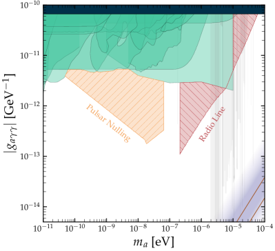
Figure 1: Parameter space in which bound axions could induce a periodic nulling of (orange), or an observable radio line from (red), the three pulsars studied in this work (see Fig. 3 in Supplemental Material (SM) for the constraints derived from individual pulsars). Shown for reference is the QCD axion band (purple), constraints from indirect astrophysical searches [41, 42, 43, 44, 45, 46, 47, 48, 49, 50, 51, 52, 28] (teal), CAST [53] (blue), and axion haloscopes [54, 55, 56, 57, 58, 59, 60, 61, 62, 63, 64, 65, 66, 67, 68, 69, 70, 71] and radio line searches in neutron stars [20, 25] (grey; shown with opacity to highlight assumption that axions are dark matter) .

I Axion Production from the Polar Cap

Axions are produced via spacetime fluctuations in $\vec{E}(\vec{x})\cdot\vec{B}(\vec{x})$, which enters as a source term in the axion’s equation of motion. Thus, in order to understand the axion production rate (and, consequently, the growth and evolution of the axion cloud), one must first understand the electrodynamic processes driving the fluctuations in $\vec{E}\cdot\vec{B}$.

In the absence of a dense axion field, the dynamics of the polar cap are expected to proceed as follows [72, 73, 74]. First, the component of the electric field parallel to the magnetic field, $E_{||}$, extracts charges from the star; at this point, the charges cannot screen the induced electric field. The charges are therefore accelerated by $E_{||}$ to high Lorenz factors, $\gamma\sim 10^{5}-10^{7}$, emitting high-energy curvature radiation along the magnetic field lines. These curvature photons travel a finite distance before pair producing in the strong magnetic field; the secondary plasma population is re-accelerated, radiating synchrotron and curvature photons, and producing a subsequent generation of $e^{\pm}$ pairs. This process proceeds until the plasma is sufficiently dense to screen the induced electric field, driving $E_{||}$ to zero. The oscillations of the plasma during this dynamical screening process are expected to generate the coherent radio emission observed from pulsars (see e.g.  [75]). Since the plasma streams relativistically along the magnetic field lines, the screening is only temporary, and $E_{||}$ returns to its original value as the plasma leaves the polar cap. This process, consisting of an ‘open phase’ (occurring prior to pair production when the gap is effectively vacuum) and a ‘closed phase’ (occurring when the gap is filled with a plasma that screens $E_{||}$), is quasi-periodic, with the characteristic timescale on the order of $\tau\sim\left({\rm few}-\mathcal{O}(10)\right)\times\tau_{\rm open}$, where $\tau_{\rm open}\sim\mathcal{O}(10^{-7}\,{\rm s})$ is the light crossing time of the gap.

The production of axions in the polar caps has been studied using both a semi-analytic model and a kinetic plasma simulation [28]. Here, in order to obtain analytic estimates for the axion production rate, we adopt the following simplifying assumptions: (1) $E_{||}$ is only non-zero in a cylindrical volume about the polar cap (with radius $r_{\rm pc}$ and height $h_{\rm gap}$); (2) it is constant and uniform for one light crossing time $\tau_{h}$, fixed to a value of $\zeta\times\vec{E}_{\rm max}$, where $\zeta\sim\mathcal{O}(1)$ and $E_{\rm max}\sim\rho_{GJ}\times h_{\rm gap}$, with $\rho_{\rm GJ}\sim-2\vec{B}\cdot\vec{\Omega}$ being the Goldreich-Julian (GJ) charge density [76]; (3) the dynamical screening of $E_{||}$ occurs over a period $\tau_{\rm close}\sim 10\times\tau_{h}$. We further assume the magnetic field is dipolar, implying the polar cap radius $r_{\rm pc}\simeq R_{\rm NS}\sqrt{R_{\rm NS}\,\Omega}$, where $R_{\rm NS}$ is the radius of the neutron star and $\Omega$ its rotational frequency. The gap height can be computed using the mean free path of curvature photons, and is given by [77, 78]

$$h_{\rm gap}\sim 12\,{\rm m}\,\left(\frac{R_{c}}{10^{7}\,{\rm cm}}\right)^{2/7}\tilde{\Omega}^{-3/7}\,\tilde{B}_{0}^{-4/7}\,,$$ (1)

where $R_{c}\simeq 9\times 10^{7}{\rm cm}\,(\theta_{\rm pc}/\theta)\sqrt{P}$ is the radius of curvature of the field lines (with with $P$ being the pulsar rotational period in seconds, and $\theta$ and $\theta_{\rm pc}$ defining the colatitude of the footprint of the magnetic field line and the polar cap boundary), and where ${B}_{0}$ is the surface magnetic field of the pulsar, and the $\tilde{X}$ notation implies the quantity $X$ is normalized to that of the Crab [80, 81] (see SM). In estimating $h_{\rm gap}$ we take $\theta\sim\theta_{\rm pc}/2$.

We focus first on light axions whose de Broglie wavelength is larger than the gap height $\lambda_{a}\gg h_{\rm gap}$ (see SM for an analogous expression when $\lambda_{a}\ll h_{\rm gap}$). The rate at which axions extract energy from the electromagnetic fields is directly related to the Fourier transform of $\vec{E}\cdot\vec{B}$ (see SM), and is approximately given by [27, 28]

$$\frac{dE_{\rm inj}}{dt} \sim \zeta^{2}\frac{g_{a\gamma\gamma}^{2}\,m_{a}^{3}}{810}\,r_{\rm pc}^{4}\,h_{\rm gap}^{5}\,B_{0}^{4}\,\Omega^{2}\,,$$ (2)

The fraction of this energy that contributes to the local energy density of axions in the polar gap can be be estimated using the density profiles derived in [29]. Assuming the cloud grows linearly on long timescales, Eq. 2 can be used to estimate the axion energy density at the surface of the neutron star after a time $t$, which is roughly given by

$$\epsilon_{0}(t)\sim\frac{3}{16\pi\,r_{\rm NS}^{3}}\times t\times\frac{dE_{\rm inj}}{dt}\,\\[5.0pt] \sim 5\times 10^{23}\,\frac{{\rm GeV}}{\rm cm^{3}}\,g_{-12}^{2}\,m_{-8}^{3}\,\tilde{t}_{\rm age}\,\tilde{B}_{0}^{8/7}\,\tilde{\Omega}^{8/7}\,,$$ (3)

where $\tilde{t}_{\rm age}$ is the age of the pulsar normalized to the Crab [80, 81], and we have introduced the notation $g_{X}=g_{a\gamma\gamma}/10^{X}\,{\rm GeV^{-1}}$ and $m_{X}=m_{a}/10^{X}\,{\rm eV}$. Eq. 3 is found to produce good agreement with the calculations of [28], and illustrates that in the absence of energy losses the axion cloud can reach large densities across a range of parameter space.

We now turn our attention toward understanding the interplay between the electrodynamics of the gap and the growing axion field, focusing in particular on the extent to which the axion can alter the electrodynamics responsible for driving radio emission. We divide our discussion into two regimes: a majority of this work focuses on the scenario when the axion field can be treated as coherent over the scale of the gap height ($\lambda_{a}\gg h_{\rm gap}$), but we also include a brief discussion on the implications of heavier axions.

II The impact of light axions ($\lambda_{a}\gtrsim h_{\rm gap}$)

We begin by considering the case of light axions whose de Broglie wavelength is much larger than the gap height $h_{\rm gap}$. Here, axions can be treated as coherent over the spatial and temporal scales governing particle acceleration and pair production – this allows us to discuss the modification to the gap dynamics under the assumption that the derivative of the axion is approximately constant over the spatial and temporal scales of interest. All expressions derived in this section should be understood to be valid exclusively in this limit.

The quantitative behavior of the discharge process can be understood using what is known as the discharge parameter, defined as $\alpha\equiv j_{||}/\rho_{\rm GJ}$, where $j_{||}$ is the current parallel to the magnetic axis; when $0\leq\alpha<1$, the charges extracted from the surface are able to supply a sufficient current to screen $E_{||}$ without the need for pair production, while vacuum gaps with non-zero $E_{||}$ (which subsequently induce quasi-periodic pair production) are expected to appear along field lines containing discharge parameters $\alpha\geq 1$ or $\alpha<0$ (see e.g. [82, 79]).

One can use the axion-modified Maxwell’s equations to understand how a dense axion field can alter the discharge process; these equations are given by [83]:

$$\nabla\cdot\vec{E} =\rho-g_{a\gamma\gamma}\vec{B}\cdot\nabla a\,,$$ (4)

$$\nabla\times\vec{B}-\dot{\vec{E}} =\vec{j}+g_{a\gamma\gamma}\dot{a}\vec{B}+g_{a\gamma\gamma}\nabla a\times\vec{E}\,,$$ (5)

$$\nabla\cdot\vec{B} =0\,,$$ (6)

$$\dot{\vec{B}}+\nabla\times\vec{E} =0\,.$$ (7)

The modified form of Gauss’ and Ampere’s law show that the presence of a background axion field generates an effective charge density $\rho_{a}=-g_{a\gamma\gamma}\vec{B}\cdot\nabla a$, and an effective current density $\vec{j}_{a}=g_{a\gamma\gamma}\dot{a}\vec{B}+g_{a\gamma\gamma}\nabla a\times\vec{E}$, which oscillate on the timescale $\tau_{a}=2\pi/\omega_{a}$. The effective charge and current densities induce corrections of the discharge parameter of the form

$$\alpha_{\rm eff}=\frac{j_{||}+j_{a,||}}{\rho_{\rm GJ}+\rho_{a}}\sim\frac{j_{||}}{\rho_{\rm GJ}}\left(1+\mathcal{O}(1)\times\frac{\rho_{a}}{j_{||}}\right)\,,$$ (8)

where in the last step we assumed that the axion field is sufficiently small to be treated as a perturbation, and that axions are semi-relativistic (for gravitationally bound axions near the neutron star surface, $k_{a}\sim m_{a}/3$ – see SM), implying $j_{a,||}\sim\mathcal{O}(1)\,\rho_{a}$. In the event that $\rho_{a}/\rho_{\rm GJ}\sim\mathcal{O}(10)\,\%$, the oscillation in the axion field can periodically drive $\alpha_{\rm eff}$ above and below the pair production threshold, inducing a periodic nulling in the radio emission – this is the primary observable effect that we identify as arising for small axion masses.

The question that remains is whether the axion can reach the large field values needed to induce sizable oscillations in $\alpha_{\rm eff}$. In order for this to occur, the axion density must be comparable to the GJ charge density, i.e. $\rho_{a}\sim\xi\rho_{\rm GJ}$, where the factor $\xi\sim\mathcal{O}(0.1)$ has been introduced to account for the uncertainty in the back-reaction threshold. This comparison allows one to derive the axion energy density when back-reaction becomes relevant – this is given by

$$\epsilon_{\rm br} \sim \xi^{2}\frac{2\Omega^{2}m_{a}^{2}}{g_{a\gamma\gamma}^{2}k_{a}^{2}}\,$$

$$\sim 5\times 10^{20}\,\frac{{\rm GeV}}{{\rm cm^{3}}}\,\tilde{\Omega}^{2}\,\left(\frac{10^{-12}\,{\rm GeV^{-1}}}{g_{a\gamma\gamma}}\frac{\xi}{0.1}\right)^{2},$$

where we have expressed the axion field in terms of its local density with an arbitrary phase $a\simeq\sqrt{2\epsilon_{a}}/m_{a}e^{i(\vec{k}_{a}\cdot x-\omega t)}$.

In order to determine whether the typical densities around pulsars can reach values near $\epsilon_{\rm br}$, one must simultaneously solve the axion’s equation of motion, Maxwell’s equations, and the Vlasov equation governing the distribution functions of electrons and positrons – such a treatment is highly non-trivial and would require state-of-the-art simulations. In order to simplify the discussion, we instead work in the limit where the axion can be treated as a small perturbation to the electrodynamics governing the discharge (which is valid so long as $\epsilon_{a}\lesssim\epsilon_{\rm br}$) – this allows us to independently compute the rate at which energy is injected into the axion cloud (Eq. 2) and the rate at which energy is dissipated from the cloud. The maximum allowed axion density, which we refer to as the saturation density $\epsilon_{\rm sat}$, is then determined by equating the rate of energy injection and dissipation.

Within this treatment, two conditions must be met in order for pulsar nulling to occur:

• The saturation density must be larger than the back-reaction density, $\epsilon_{\rm sat}\gg\epsilon_{\rm br}$. This ensures that energy losses do not prevent the axion cloud from reaching $\epsilon_{\rm br}$.

• The back-reaction density must be obtainable within the lifetime of the pulsar. Assuming the former condition is met, this roughly corresponds to the requirement that $\epsilon_{0}(t=t_{\rm today})\sim t_{\rm age}\times d\epsilon_{\rm inj}/dt\gtrsim\epsilon_{\rm br}$, where $d\epsilon_{\rm inj}/dt$ is the growth rate of the energy density at present time .

A comparison between Eq. II and Eq. 3 illustrates that in the absence of energy losses, the axion cloud can indeed reach back-reaction densities across a sizable range of parameter space – thus, the second condition outlined above can certainly be met for some pulsars. The question remains of whether axions in the polar cap can efficiently dissipate their energy, causing the growth of the axion field to quench before reaching the point of back reaction.

Axions can either directly radiate photons, or dissipate energy into the plasma via the axion-induced electric fields. The former process requires the effective plasma frequency [84], $\omega_{p,{\rm eff}}\equiv(\left<\omega^{2}_{p}/\gamma^{3}\right>)^{1/2}$ (where $\left<\,\right>$ denotes the average over the distribution functions and the species present in the plasma, $\gamma$ is the Lorentz factor, and the plasma frequency of a single species $s$ is defined as $\omega_{p,s}^{2}\equiv q_{s}^{2}n_{s}/m_{s}$, with $q_{s},n_{s},$ and $m_{s}$ the charge, number density, and mass), to be less than the axion energy, a condition which must hold over the oscillation timescale of the axion. During the open phase of the gap, $\omega_{p,{\rm eff}}\lesssim 10^{-12}$ eV, and this increases exponentially after the onset of pair production, saturating when no more pairs can be produced. Since photons can only be produced when $\omega_{a}\geq\omega_{p,{\rm eff}}$ (which is typically only satisfied prior to pair production), the condition for on-shell photon production translates into the condition that the axion oscillation timescale is less than the light crossing time of the gap, $\tau_{a}\lesssim h_{\rm gap}$. Clearly, this condition is nearly synonymous with the condition that $\lambda_{a}\lesssim h_{\rm gap}$, and thus at low axion masses the only viable dissipation channel arises when the axion-induced electric fields dissipate energy into the local plasma. We return to the discussion of photon production from heavy axions in the following section.

In the SM, we derive the leading order correction from the axion to the electric field, which is given by

$$\vec{E}_{a}\sim g_{a\gamma\gamma}\frac{\sqrt{2\,\epsilon_{a}}}{m_{a}}\vec{B}\,e^{-im_{a}t}\times\mathcal{F}(m_{a},h_{\rm gap},\omega_{p})\,.$$ (10)

Here, we have introduced a factor $\mathcal{F}$ to capture the in-medium suppression, with $\mathcal{F}=1$ in a uniform vacuum and $\mathcal{F}\sim(m_{a}/\omega_{p})^{2}\ll 1$ in a dense uniform plasma. The suppression can be partially alleviated during the open phase of the gap, instead scaling like the fractional volume of vacuum within a de Broglie wavelength; e.g. , for $r_{\rm pc}\gg\lambda_{a}\gg h_{\rm gap}$, $\mathcal{F}\sim(h_{\rm gap}/\lambda_{a})$ (see SM for additional limiting cases).

Depending on the relative sign of $\vec{E}_{a}$ (with respect to $\vec{E}_{||}$), the axion-induced electric field will either cause the primary $e^{\pm}$ to accelerate slightly more, or slightly less. In the event that the current does not dissipate energy, the oscillatory nature of the induced electric field would cause the energy loss to average to zero, i.e. $\left<\vec{j}_{e}\cdot\vec{E}_{a}\right>=0$. The charges, however, emit curvature radiation, and this provides an energy ‘sink’ that does not cancel when time-averaged. As shown in the SM, the (time-averaged) rate at which axions lose energy is given by

$$\left<\frac{dE_{\rm dis}}{dt}\right> \sim \frac{g_{a\gamma\gamma}^{2}}{14\pi}\,\epsilon_{a}\,B_{0}^{5}\,\Omega^{3}\,\frac{e^{5}\,h_{\rm gap}^{9}\,r_{\rm pc}^{2}}{m_{e}^{4}\,R_{c}^{2}}\,.$$ (11)

Equating the injection and dissipation rates, i.e. Eq. 11 and Eq. 2, one arrives at the saturation density

$$\epsilon_{\rm sat} \sim 8\times 10^{19}\,\frac{\rm GeV}{\rm cm^{3}}\,\zeta^{2}\,m_{-8}^{3}\,\tilde{B}^{9/7}\,\tilde{\Omega}^{9/7}\,,$$ (12)

which we note is also independent of axion-photon coupling. By comparing $\epsilon_{\rm sat}$, $\epsilon_{\rm br}$, and $\epsilon_{0}(t)$, one can determine for any pulsar whether nulling is expected to occur. In Fig. 1 we highlight the parameter space for which this phenomenon may occur (see SM).

III The Impact of Heavy Axions $(\lambda_{a}\lesssim h_{\rm gap})$

There are three primary differences that arise when one considers the implications of heavier axions (i.e. those with $\lambda_{a}\ll h_{\rm gap}$). First, high-mass axions are produced by rapid small scale fluctuations in the plasma – since the amplitude of these fluctuations are much smaller than the vacuum field, the production rate is suppressed relative to the low-mass limit. Second, the axion field is now incoherent over the gap, meaning one must account for the stochasticity of the axion phase. This heavily suppresses the effect of the axion on the electrodynamics; for example, the induced electric field at any point can accelerate/decelerate the ambient charges to the same degree as before, however the net voltage drop across the gap is only non-zero because the cancellation between phases is not exact. In the SM we provide a more detailed discussion of these differences, and derive analogous expressions in the high mass limit for $\epsilon_{\rm br}$, $\epsilon_{0}(t)$, and $\epsilon_{\rm sat}$. In particular, we show that the incoherence of the axion field leads to a larger back-reaction density and a suppression of the energy losses due to curvature radiation. We further argue that at large masses, an axion density of $\epsilon\sim\epsilon_{\rm br}$ does not imply the existence of pulsar nulling.

The final distinction arises from the fact that the oscillation timescale of the axion field is now sufficiently fast to produce on-shell electromagnetic radiation during the open phase of the gap. The presence of on-shell radiation provides a direct observable in the high mass regime – namely, a narrow radio line emanating from the polar cap. In the SM, we show the average energy loss to radio emission is roughly given by

$$\frac{dE_{\gamma}}{dt} \sim \frac{1}{4\pi}\,\frac{g_{a\gamma\gamma}^{2}\,a^{2}\,B_{0}^{2}}{\omega^{2}}\,\tau_{\rm duty}\simeq\frac{g_{a\gamma\gamma}^{2}\,\epsilon_{a}\,B_{0}^{2}}{2\pi\,m_{a}^{4}}\tau_{\rm duty}\,,$$ (13)

where we have incorporated a suppression $\propto\lambda_{a}^{3}/V_{\rm gap}$ due to the incoherency of the radiating axion cloud (see SM). $\tau_{\rm duty}\sim 1/10$ is a duty cycle factor to account for the fact that emission only occurs when the gap is open. As discussed in the SM, the radio line will be heavily beamed; this is a consequence of the fact that the return current layers have dense plasma, and thus they behave as conducting walls which serve to reflect and confine the radiation. Assuming that the axion coupling is sufficiently large that the back-reaction density is reached, i.e. $g_{a\gamma\gamma}\geq g_{P}^{\rm min,br}$, where $g_{P}^{\rm min,br}$ is the minimum coupling required for pulsar $P$ to produce an axion cloud with density $\epsilon_{\rm br}$, and that beaming confines the emission to an angular opening of the size of the polar cap (i.e. $\theta_{\rm max}\sim r_{pc}/R_{\rm NS}$, see SM), we infer an observable flux density of

$$S_{\gamma}(g_{a\gamma\gamma} \geq g_{P}^{\rm min,br})\equiv\frac{dE_{\gamma}/dt}{d\Omega\,\mathcal{B}\,d^{2}\,}$$

$$\sim 38{\rm\,Jy}\,\Big{(}\frac{\xi}{0.1}\,\frac{2\,{\rm{kpc}}}{d}\Big{)}^{2}\,\frac{\tilde{B}_{0}^{-2/7}\,\tilde{\Omega}^{-9/7}}{m_{-6}}\,,$$

where we set the bandwidth to be $\mathcal{B}=m_{a}/50$; notice that for reasonable parameters this flux can greatly exceed the intrinsic radio flux of the pulsar. At couplings $g_{a\gamma\gamma}\leq g_{P}^{\rm min,br}$, the flux density scales as $S_{\gamma}\propto g_{a\gamma\gamma}^{4}$.

IV Results and Conclusions

We have chosen to use the Crab pulsar throughout this work as a reference, since it is well-studied, the gap dynamics are effectively one-dimensional [79], and the high rotational frequency implies a large axion production rate. There exist pulsars, however, which are more favorable targets to observe both pulsar nulling and non-resonant radio emission – we thus use the ATNF catalogue to identify better targets for both observables. In the case of pulsar nulling, the Crab pulsar is primarily limited by the efficient energy dissipation – as such, we maximize the ratio of $\epsilon_{\rm sat}/\epsilon_{\rm br}\propto B^{9/7}/\Omega^{5/7}$; in the case of radio line emission for high-mass axions, we instead sort pulsars by the ratio of $(B\,\Omega)^{-2/7}/d^{2}$ (and require radio observations at multiple frequencies). We further enforce that the inferred magnetic field remain below the Schwinger field strength, the pulsar is not a millisecond pulsar, and the spin-down rate $\dot{E}>10^{34}$ erg/s (the latter condition being a rough estimator for when pair cascades are one-dimensional). Among the optimal candidates for pulsar nulling is J1119-6127, while for radio emission we find the preferred pulsar is B1055-52; the parameters for each pulsar are given in Tab. 1. In the SM we identify the parameter space for which back reaction, pulsar nulling, and observable radio emission would arise for each of the three pulsars – these results are combined in Fig. 1 in order to provide the reader with an idea of the axion parameter space that could be explored using future observations.

This work represents an initial investigation into previously unknown phenomena; the primary goals of this manuscript were to $(i)$ provide rough estimates illustrating when back-reaction can occur, and $(ii)$ identify the most robust signatures that can arise when such densities are achieved. As shown in Fig. 1, both pulsar nulling and non-resonant axion-induced radio emission from the polar cap region may provide sensitive probes of axions across a wide range of unexplored parameter space. The complexity of axion-electrodynamics in these environments necessitates rigorous follow-ups using state-of-the-art numerical simulations (see e.g.  [75, 85]) which self-consistently include axion back-reaction; this highly non-linear regime can potentially produce striking new signatures, such as unexpected long-term suppression of the radio emission and shifts in the neutron star death line.

V Acknowledgments

The authors would like to thank Georg Raffelt, Edoardo Vitagliano, Jamie McDonald, Ani Prabhu, Thomas Schwetz, Dion Noordhuis, Andrew Shaw, and Cole Miller for their useful discussions. AC acknowledges the hospitality of the Flatiron Center for Computational Astrophysics during the initial stages of this project. SJW acknowledges support from a Royal Society University Research Fellowship (URF-R1-231065), and through the program Ramón y Cajal (RYC2021-030893-I) of the Spanish Ministry of Science and Innovation. This article/publication is based upon work from COST Action COSMIC WISPers CA21106, supported by COST (European Cooperation in Science and Technology). This work was supported by a grant from the Simons Foundation (MP-SCMPS-00001470) to AP. The work of TJ was supported in part by NSF grant PHY-2309634.

Supplementary Material for Axion-Induced Pulsar Nulling and Non-Resonant Radio Emission
Andrea Caputo, Samuel J. Witte, Alexander Philippov, Ted Jacobson

Below, we provide additional details justifying some of the approximations, and outlining the derivations of various quantities quoted in the main text. These include: a look at the velocity distribution of the axion cloud near the neutron star surface, the derivation of the axion-induced electric field, a derivation of the axion production rate, back-reaction density, and energy dissipation rate (both at high and low axion masses), a look at the impact of magneto-rotational spin-down, details on the sensitivity analysis, and a discussion on possible resonant transitions during the phase of pair production.

Appendix A Velocity distribution near the neutron star

Throughout the main text we have used the approximation that the axion phase space in the gap itself is dominated by characteristic axion momenta $k_{a}\sim m_{a}/3$. In order to justify this approximation we compute the initial axion spectrum for the Crab pulsar, sample momenta from the derived production rate (in units of number of axions per unit k-mode), and follow the evolution of these sampled axion bound states for a timescale on the order of $t\sim 1\,\rm s$ (corresponding to $3\times 10^{3}$ neutron star crossing times). These trajectories are traced following treatment of [29]. From the sampled trajectories, we draw a spherical surface at some radius $r$ around the neutron star and determine the crossing points of each of the trajectories. Each crossing point is re-weighted using the procedure outlined in [29]. We plot the normalized distribution of weighted samples in Fig. 2.

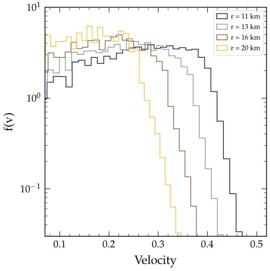
Figure 2: Normalized axion velocity distribution $f(v)$ as a function of velocity evaluated at four different radii, averaged over the all angles. This distribution is used to justify the the approximation $k_{a}\sim m_{a}/3$ near the neutron star surface.

Appendix B Axion-induced Electric Field

Here, we provide additional details outlining the derivation of the induced electric field and the energy dissipation mechanisms. We begin by following Ref. [86] in identifying the transition amplitude from an electron between initial $\left.|i\right>$ and final $\left.|f\right>$ states at zeroth order in axion-photon coupling:

$$\mathcal{A}=i\left<f|\int d^{4}x\mathcal{H}_{I}(x)|i\right>=i\int d^{4}x\,J^{\mu}(x)A_{\mu}^{\rm ext}(x)\,,$$ (15)

where we have defined the vector potential induced by an external electromagnetic field, and we have defined $J^{\mu}\equiv e\left<f|\bar{\psi}\gamma^{\mu}\psi|i\right>$. We can determine the analogous expression at second order from the axion-induced electric field as

$$\mathcal{A}=\frac{(-i)^{2}}{2!}\left<f|T\int d^{4}x\,\int d^{4}y\mathcal{H}_{I}(x)\mathcal{H}_{I}(y)|i\right>$$ (16)

were $T$ is the time-ordered product, and $H_{I}$ includes the axion and fermion interaction terms. This amplitude can be re-expressed as

$$\mathcal{A}=-i\int d^{4}xJ^{\mu}(x)A_{\mu}^{\rm ind}(x),$$ (17)

where the induced vector potential is given by

$$A_{\mu}^{\rm ind}(x)=ig_{a\gamma\gamma}\int d^{4}yD_{\mu\nu}(x-y)\partial_{\rho}a(y)\tilde{F}^{\rho\nu}(y)$$ (18)

with $D_{\mu\nu}$ being the photon propagator. At this point our derivation deviates from that in  [86], as we must consider the dressed propagator in medium, which is given (in the Feynman gauge) by

$$D_{\mu\nu}(x-y)=\int\frac{d^{4}q}{(2\pi)^{4}}\frac{-ig_{\mu\nu}}{q^{2}-\Pi_{L,T}}\,e^{-iq(x-y)}\,,$$ (19)

with $\Pi_{L,T}$ the longitudinal and transverse polarization tensors. For a non-thermal plasma in the limit $q\rightarrow 0$, these are given by $\Pi_{L,T}\simeq\omega_{p}^{2}$ [87, 88], with $\omega_{p}$ the plasma frequency. In the limit that $q^{2}\sim m_{a}^{2}\ll\omega_{p}^{2}$, the $d^{4}q$ integration just gives $(2\pi)^{4}\delta^{(4)}(x-y)/\omega_{p}^{2}$, so the induced vector potential simplifies to

$$A_{\mu}^{\rm ind}(x)=ig_{a\gamma\gamma}\frac{\partial^{\rho}a(x)\tilde{F}_{\rho\mu}(x)}{\omega_{p}^{2}}\,.$$ (20)

Note that this ‘contact interaction’ approximation is valid so long as $k\sim m_{a}\ll\omega_{p}$, which is valid for most of the magnetosphere of the Crab pulsar, so long as $m_{a}\lesssim 10^{-5}$ eV. Taking the non-relativistic limit we see that the dominant contribution to the electromagnetic field is given by

$$\vec{E}^{\rm ind}=-\partial_{t}\vec{A}^{\rm ind}\simeq ig_{a\gamma\gamma}\Big{(}\frac{m_{a}}{\omega_{p}}\Big{)}^{2}\frac{\sqrt{2\,\epsilon_{a}(r)}}{m_{a}}\vec{B}\,e^{i(k_{a}\cdot r-m_{a}t)},$$ (21)

where we recognize the typical in-medium suppression factor $(m_{a}/\omega_{\rm pl})^{2}$ (see e.g. [89] for a comparison in the context of dark photons). We can also compute the analogous expression for the induced magnetic field, which is given by

$$\vec{B}^{\rm ind} = -\nabla\times\vec{A}^{\rm ind}$$

$$\sim ig_{a\gamma\gamma}\Big{(}\frac{k_{a}}{\omega_{p}}\Big{)}^{2}\frac{\sqrt{2\,\epsilon_{a}(r)}}{m_{a}}E_{||}\,e^{i(k_{a}\cdot r-m_{a}t)}(\hat{x}+\hat{y})$$

where we have assumed $\nabla\times\vec{B}\simeq 0$ and $\vec{E}\simeq E_{||}\hat{z}$ in the polar cap, and $\partial_{x,y}(aE_{||})\sim kaE_{||}$.

The in-medium effect leads to a powerful suppression of the induced electric and magnetic fields when $m_{a}\ll\omega_{p}$. However, during the ‘open phase’ of the gap has an effective plasma frequency on the order $\omega_{p}/\gamma^{3/2}\lesssim 10^{-12}$ eV, and thus we expect the dominant energy losses to arise during this short-lived phase.

In order to analyze the behavior of the induced electric field during the open phase of the gap, we assume one can treat the gap itself as being pure vacuum surrounded by a sharp boundary of dense plasma; while this is slightly over-simplified, it allows us to obtain rough estimates of the induced electric field and the effect of this field on the system. Re-solving Eq. 18 with this geometry we find

$$\vec{E}^{\rm ind}\simeq ig_{a\gamma\gamma}\mathcal{F}(m_{a},h_{\rm gap},\omega_{p})\frac{\sqrt{2\,\epsilon_{a}(r)}}{m_{a}}\vec{B}\,e^{i(k_{a}\cdot r-m_{a}t)}\,,$$ (23)

where, assuming $\omega_{p}\gg m_{a}$, one finds the suppression factor to be

$$\mathcal{F}\sim\begin{cases}1\hskip 1.42271pt&\lambda_{a}\ll h_{\rm gap},r_{\rm pc},R_{\rm NS}\\ \left(\frac{h_{\rm gap}}{\lambda_{a}}\right)\hskip 1.42271pt&h_{\rm gap}\ll\lambda_{a}\ll r_{\rm pc},R_{\rm NS}\\ \left(\frac{h_{\rm gap}r_{\rm pc}^{2}}{\lambda_{a}^{3}}\right)&h_{\rm gap},r_{\rm pc}\ll\lambda_{a}\ll R_{\rm NS}\\ \end{cases}\,.$$ (24)

Appendix C The Low Axion Mass Regime

In this section we provide extra details about the derivation of the axion production rate, the back-reaction density derivation and the energy loss in the small mass regime, i.e $\lambda_{a}\gg h_{\rm gap}$.

C.0.1 Axion Production

We start by outlining the derivation of the energy injection rate and the density of the axion cloud at the neutron star surface. Additional details and discussion can be found in [28].

Starting from the axion’s equation of motion, $(\Box+m_{a}^{2})a(x)=-g_{a\gamma\gamma}\vec{E}(x)\cdot\vec{B}(x)$, one can show that rate at which energy is injected into axions is given by [28]

$$\frac{dE_{\rm inj}}{dt}=\frac{1}{2(2\pi)^{3}\tau}\int d^{3}k|\tilde{\mathcal{S}}(\vec{k})|^{2}\,,$$ (25)

where we have defined the source term for axions

$$\tilde{\mathcal{S}}(\vec{k})=-g_{a\gamma\gamma}\int d^{4}x\,e^{ik\cdot x}\,\vec{E}(x)\cdot\vec{B}(x)\,,$$ (26)

and $\tau$ is defined to be the characteristic period of the gap collapse process. It is then clear that in order to compute the axion production rates one needs the Fourier transform (FT) of the source term $\vec{E}(x)\cdot\vec{B}(x)$. We also note that in defining the FT of the source, we have implicitly enforced the on-shell condition $\omega_{a}^{2}=k_{a}^{2}+m_{a}^{2}$.

In order to make quantitative estimates one the needs to specify $\vec{E}(x)\cdot\vec{B}(x)$ and its temporal evolution. Within the simplifying assumptions outlined in the main text, and working in the limit $m_{a}/(2\pi)\ll\tau^{-1}$ (the opposing limit will be discussed below), the typical energy injection rate can be estimated using Eq. 25, and is given by

$$\frac{dE_{\rm inj}}{dt} \sim \frac{g_{a\gamma\gamma}^{2}}{2(2\pi)^{3}}\underbrace{\frac{4\pi\,m_{a}^{3}}{81}}_{d^{3}k}\underbrace{\pi^{2}\,r_{\rm pc}^{4}h_{\rm gap}^{2}}_{V_{\rm gap}^{2}}\frac{\tau_{\rm open}^{2}}{\tau}\zeta^{2}B_{0}^{2}\underbrace{4\,B_{0}^{2}\Omega^{2}h_{\rm gap}^{2}}_{E_{\rm max}^{2}}$$ (27)

$$\sim \zeta^{2}\frac{g_{a\gamma\gamma}^{2}\,m_{a}^{3}}{810}\,r_{\rm pc}^{4}\,h_{\rm gap}^{5}\,B_{0}^{4}\,\Omega^{2},$$

where we have assumed $\tau_{\rm open}\sim h_{\rm gap}$ and $\tau=\tau_{\rm open}+\tau_{\rm closed}\sim 10\,h_{\rm gap}$.

The characteristic density at the surface is obtained by noting that the density profile outside the star scales as $\epsilon_{a}\propto r^{-4}$, and is roughly constant within the star. Using this profile, one can estimate the fraction of the energy being injected into bound states in radii $r\in[r_{\rm NS},r_{\rm NS}+h_{\rm gap}]$; dividing off by the appropriate volume element yields Eq. 3.

C.0.2 Back-reaction density

In order to compute the back-reaction density we need to evaluate the axion cloud effective charge density, $\rho_{a}=-g_{a\gamma\gamma}\vec{B}\cdot\nabla a$ and compare it with the GJ density, $\rho_{\rm GJ}$. Since particle acceleration and pair production is nearly one-dimensional, we are interested in comparing $\rho_{\rm GJ}$ with the value of $\rho_{a}$ averaged over the open phase of the gap and over a characteristic bundle of field lines. In the low mass regime ($\lambda_{a}\gg h_{\rm gap}$), the axion field is approximately uniform (both spatially and temporally during the open phase of the gap), and thus this trivially yields

$$\frac{1}{h_{\rm gap}\,\tau_{\rm open}}\int dt\int_{R_{\rm NS}}^{R_{\rm NS}+h_{\rm gap}} dz \nabla a=a(R_{\rm NS}+h_{\rm gap})-a(R_{\rm NS})$$ (28)

$$\simeq \frac{\sqrt{2\epsilon_{a}}}{m_{a}}k_{a}\,\cos(m_{a}\,t+\delta),$$

where we introduced a random phase $\delta$ for the axion field. Imposing $\rho_{a}\sim\xi\rho_{\rm GJ}$, where the factor $\xi\sim\mathcal{O}(0.1)$ has been introduced to account for the uncertainty in the back-reaction threshold, and using Eq. 28 for the axion gradient, one finds Eq. II of the main text

$$\epsilon_{\rm br} \sim \xi^{2}\frac{2\Omega^{2}m_{a}^{2}}{g_{a\gamma\gamma}^{2}k_{a}^{2}}\,$$ (29)

$$\sim 5\times 10^{20}\,\frac{{\rm GeV}}{{\rm cm^{3}}}\,\left(\frac{\Omega}{190.4{\rm Hz}}\frac{10^{-12}\,{\rm GeV^{-1}}}{g_{a\gamma\gamma}}\frac{\xi}{0.1}\right)^{2}.$$ (30)

C.0.3 Energy dissipation rate

Here we compute the energy loss of charges due to curvature radiation. We recall this is a crucial quantity to compute the saturation density (Eq. 12), as curvature radiation provides an energy ‘sink’ for the axion field. The rate of energy loss per particle due to curvature radiation is given by  [90]

$$\dot{E}_{e^{\pm}}\simeq\frac{3e^{2}}{2R_{c}^{2}}\gamma^{4}\,.$$ (31)

Neglecting energy losses, the differential change in $\gamma$ as a function of distance $s$ is given by $d\gamma(s,\vec{E})/ds\sim e|\vec{E}|/m_{e}$. To compute the energy losses from the axion field, we can first compute the total energy dissipated across the gap in the form of curvature during a single vacuum phase

$$\frac{dE_{\rm dis}}{dt} \sim \pi r_{\rm pc}^{2}\,n_{\rm GJ}\,\int_{0}^{h_{\rm gap}}ds\,\dot{E}_{e^{\pm}}(s)\,.$$ (32)

Writing the electric field as a bare component (assumed to be linearly proportional to the height) and a constant perturbation due to the axion, i.e. $\vec{E}_{0}(s)\pm\vec{E}_{a}$ and therefore $\gamma\sim\frac{e}{m_{e}}\Big{(}\frac{E_{0}s^{2}}{2\,h_{\rm gap}}+E_{a}s\Big{)}$ [90], one can expand Eq. 32 in powers of $\epsilon=|\vec{E}_{a}|/|\vec{E}_{0}|$. Since the first order term $\propto\vec{E}_{a}$ will induce a vanishing contribution when averaged on timescales $t\gg 2\pi/m_{a}$, the leading order contribution to the energy loss arises at $\mathcal{O}(\epsilon^{2})$ – time averaging this term (and working in the limit limit $h_{\rm gap}\ll\lambda_{a}\ll r_{\rm pc}$) we arrive indeed to Eq. 11

$$\left<\frac{dE_{\rm dis}}{dt}\right> \sim \frac{g_{a\gamma\gamma}^{2}}{70\pi}\,\epsilon_{a}\,B_{0}^{5}\,\Omega^{3}\,\frac{e^{5}\,h_{\rm gap}^{9}\,r_{\rm pc}^{2}}{m_{e}^{4}\,R_{c}^{2}}\,.$$ (33)

Analogous expressions can be derived for $\lambda_{a}\gg r_{\rm pc},h_{\rm gap}$ by using the appropriate axion-induced electric field. Notice that we have included a factor of $\sim 1/10$ to account for the duty cycle of the open phase of the gap.

Appendix D The High Axion Mass Regime

The main text of the manuscript has focused primarily on deriving quantities in the low-mass limit, as in this regime the axion field can be treated as coherent over the gap, implying the impact of the axion on the electrodynamics is greatly simplified. At large masses, this is no longer true – the axion field stochastically samples random phases within the gap, implying many effects tend to cancel, or wash out. Here, we re-derive all the relevant quantities – namely, the scaling of the axion production rate, the back-reaction density, and the rate of energy dissipation – in the high mass limit..

D.0.1 Axion production rate

In general, the Fourier transform (FT) of $\vec{E}\cdot\vec{B}$ receives two contributions, one coming from the characteristic geometry of the gap, and the other coming from the small scale oscillations induced by the plasma screening process. Since oscillations can only exist on scales below the gap size, the second contribution is zero in the low mass limit (and as such has been neglected in the main text). At large axion masses, the volumetric contribution is expected to scale like $\tilde{\mathcal{S}}\propto(\lambda_{a}/L_{\rm gap})^{3}$, meaning the contribution to the axion production rate is dramatically suppressed at high masses. This effect is largely compensated, however, by the contribution arising from the small-scale oscillations in the plasma. In order to illustrate this effect, let us consider a 1-dimension toy example in which we consider a window function with a small scale oscillatory perturbation, i.e.

$$f(x)= f_{\rm geometery}+f_{\rm oscillations}$$ (34)

$$= \,\Theta(x)\Theta(L-x)+\epsilon\Theta(x)\Theta(L-x)\sin(k_{\rm osc}\,x),\,$$

where $\Theta$ is the Heaviside step function, $L$ is the length of the window function, $\epsilon$ is the size of the oscillatory perturbation, and $k_{\rm osc}$ is the wavelength of the perturbation. In the limit $k_{\rm osc}\rightarrow 0$ we recover the purely geometric contribution which is merely the size of the gap ${\rm FT}(f)_{k_{\rm osc}\rightarrow 0}\sim L$. In the alternative limit (and evaluating the FT for $k\rightarrow k_{\rm osc}$), one is instead dominated by the oscillatory contribution, finding ${\rm FT}(f)_{k_{\rm osc}\rightarrow 0}\sim L\times(\epsilon/2)$.

Returning to the case of the polar cap, the amplitude of oscillations decreases as the oscillation frequency increases (i.e. a denser plasma induces higher frequency damped oscillations in the electric field); that is to say, the normalization of the amplitude of oscillations in the previous example is in fact a function of the frequency itself, i.e. $\epsilon(\omega)$. Using the analytic derivations of the one-dimension response derived in [91], we can estimate that the amplitude of oscillations scales with the frequency approximately as $E_{||}(\omega)\propto E_{||,0}\times(\omega/\omega_{0})^{-\xi}$, with $\xi\sim 0.5$. Working in one dimension, this suggests that at large axion masses (which for non-relativistic axions implies large oscillation frequencies) one expects the Fourier transform of $\vec{E}\cdot\vec{B}$ to scale as $m_{a}^{-1/2}$; generalizing this result to three dimensions, and assuming the temporal integral in $\tilde{\mathcal{S}}$ follows similar trend to the spatial contributions, one finds that the high mass limit scales like

$$\Big{(}\frac{dE_{\rm inj}}{dt}\Big{)}_{\rm high}\sim\Big{(}\frac{dE_{\rm inj}}{dt}\Big{)}_{\rm low}\Big{(}\frac{1}{m_{a}\,L_{\rm gap}}\Big{)}^{3}\Big{(}\frac{\omega_{0}}{m_{a}}\Big{)},$$ (35)

where $\Big{(}\frac{dE_{\rm inj}}{dt}\Big{)}_{\rm low}$ is defined in Eq. 2 of the main text. In order to derive a practical expression for the evolution of the density in the high mass limit we simply extract the functional dependence of Eq. 35, and ensure continuity at the transition mass with Eq. 2. Using the parameters of the Crab, this leads to a density of

$$\epsilon_{0}(t)\sim 10^{25}\,\frac{{\rm GeV}}{\rm cm^{3}}\,g_{-12}^{2}\,\frac{\tilde{t}_{\rm age}}{m_{-6}}\,\tilde{B}_{0}^{24/7}\,\tilde{\Omega}^{24/7}\,.$$ (36)

D.0.2 Back-reaction density

We now reconsider the back-reaction density. At high masses, when the axion field is no longer coherent, the effective charge and current densities induced by the axion oscillate on scales much smaller than the gap size (and on times much smaller than the light crossing time of the gap). This implies that the average axion-induced charge and current densities tend toward zero in the limit that $m_{a}\rightarrow\infty$; an easy way to understand that this is the case is to recognize that the small scale oscillations in the electric field will leave the net voltage drop across the gap unchanged, and as such the axion is not expected to produce sizable changes to the gap collapse process. For any finite axion mass, however, there will exist a residual phase in the axion field that will not lead to a perfect cancellation. In a one-dimensional treatment, the spatio-temporal average (over the open phase of the gap) of $\nabla a$ yields

$$\frac{1}{h_{\rm gap}\,\tau}\int dt\int_{R_{\rm NS}}^{R_{\rm NS}+h_{\rm gap}}dz\nabla a\,\,\simeq\frac{\sqrt{2\epsilon_{a}}\cos(m_{a}\,t+\delta)}{m_{a}^{2}\,h_{\rm gap}\tau_{\rm open}}.$$

Taking $\tau_{\rm open}\sim h_{\rm gap}$, we find that this limit yields a suppression of $\nabla a$ scaling as $(\lambda_{a}/h_{\rm gap})^{2}$; equivalently, this corresponds to a back-reaction density in the large mass limit of

$$\epsilon_{\rm br}\simeq\xi^{2}\frac{2\,\Omega^{2}m_{a}^{4}h_{\rm gap}^{4}}{\,g_{a\gamma\gamma}^{2}},$$ (38)

which differs from the case of small axion masses by a factor $\sim m_{a}^{2}\,k_{a}^{2}\,h_{\rm gap}^{4}$. Expressing the back-reaction density in terms of the Crab parameters, one finds

$$\epsilon_{\rm br}\simeq 3\times 10^{27}\,\rm\frac{GeV}{cm^{3}}\,\Big{(}\frac{\xi}{0.1}\Big{)}^{2}\,\left(\frac{m_{-6}^{4}}{g_{-12}^{2}}\right)\,\tilde{\Omega}^{-2/7}\,\tilde{B}_{0}^{-16/7}.$$

Note that the extrapolation of Eq. D.0.2 and Eq. II to the threshold mass, i.e. where $2\pi/m_{a}=h_{\rm gap}$, leads to a discontinuity – this is a result of the fact that Eq. D.0.2 has been derived under the assumption that $\lambda_{a}\ll h_{\rm gap}$. In order to generate smooth curves across the axion parameter space (as in Fig. 1), we simply derive the mass $\bar{m}$ for which these curves cross (corresponding to $\bar{m}\sim 1.74/h_{\rm gap}$), and define a piece-wise function for smaller and larger masses using Eq. II and Eq. D.0.2, respectively.

As an aside, one may wonder why the back-reaction density has been derived by averaging the axion gradient only over an the spatial direction oriented along the magnetic axis (and over time), but does not include an average over the radial direction. For young pulsars, acceleration and pair production is nearly one-dimensional, and thus averaging only over the z direction reflects the threshold at which local pair production would be effected, while including the radial direction instead reflects the point at which pair production would globally be effected. Including the radial direction would dramatically increase the back-reaction density – we thus choose to adopt the more conservative threshold (this is conservative in that the the maximal density, which enters e.g. the computation of the radio flux, is lower), which is set by restricting to the domain where the local dynamics of pair production begins to become altered.

D.0.3 Energy dissipation rate

Finally, we turn our attention to the energy dissipation rate. The expression derived in Eq. 32 corresponds to the energy loss arising from particle acceleration. At large masses, however, the electric field oscillates on small scales, and is not expected to induce any net voltage drop across the gap; as a consequence, the induced electric field will induce no net work on the system. Nevertheless, if the axion mass is larger than the local plasma frequency, one can also directly produce on-shell photons. At small masses, this process is blocked by the presence of the plasma – this occurs since a dense plasma is produced within the oscillation timescale of the axion. At larger masses, however, the axion oscillates rapidly, and can produce on-shell radiation during the vacuum phase. In order to compute the rate of energy loss via electromagnetic emission we revisit the computation of the axion-induced electromagnetic fields, but focusing on the far-field (rather than near-field) limit. This is done by expanding the electromagnetic fields as $\vec{B}=\vec{B}_{0}+\delta\vec{B}$ and $\vec{E}=\vec{E}_{0}+\delta\vec{E}$, and re-deriving the wave equations in the absence of classical source terms, but in the presence of an axion background. The resultant solutions for the perturbed electromagnetic fields are given by

$$(\partial_{t}^{2}-\nabla^{2})\delta\vec{E} = \nabla\rho_{a}-\partial_{t}\,\vec{j}_{a},$$ (40a)

$$(\partial_{t}^{2}-\nabla^{2})\delta\vec{B} = -\nabla\times\vec{j}_{a}\,,$$ (40b)

where for simplicity we have neglected the plasma frequency (i.e strictly speaking we assume here $m_{a}\gg\omega_{p}$). These equations can be solved using Greens functions, which in the far-field limit $|\vec{x}-\vec{x}^{\prime}|/|\vec{x}|\ll 1$ give

$$\delta\vec{E}(\vec{x}) = \frac{e^{-i\omega\,t+i\omega\vec{x}}}{4\pi|\vec{x}|}\int d^{3}\textbf{x}^{\prime}e^{-i\omega\,\vec{x}\cdot\vec{x}^{\prime}/|\vec{x}|}(\nabla\rho_{a,x}(\vec{x}^{\prime})$$ (41)

$$+i\omega\,\vec{j}_{a,x}(\vec{x}^{\prime})),$$

$$\delta\vec{B}(\vec{x}) = -\frac{e^{-i\omega\,t+i\omega\vec{x}}}{4\pi|\vec{x}|}\int d^{3}\textbf{x}^{\prime}e^{-i\omega\,\vec{x}\cdot\vec{x}^{\prime}/|\vec{x}|}\,\nabla\times\vec{j}_{a,x}(\vec{x}^{\prime}),$$

where we introduced the notation $\vec{j}_{a,x}=e^{-i\omega t}\vec{j}_{a}$ and $\rho_{a,x}=e^{-i\omega t}\rho_{a}$. Taking the limit $\omega\times|x^{\prime}|\ll 1$ and integrating over the source yields

$$\delta\vec{E}(t,\vec{x}) \sim \frac{e^{-i\omega\,t+i\omega\vec{x}}}{4\pi|\vec{x}|\,\omega^{3}}(i\,\vec{k}\rho_{a,x}(\vec{k})+i\omega\,\vec{j}_{a,x}(\vec{k})),$$ (42a)

$$\delta\vec{B}(t,\vec{x}) \sim -\frac{e^{-i\omega\,t+i\omega\vec{x}}}{4\pi|\vec{x}|\,\omega^{3}}\,i\,\vec{k}\times\vec{j}_{a,x}(\vec{k}).$$ (42b)

Notice that ultimately the factor $1/\omega^{3}$ comes from the fact that in the high-mass regime the axion cloud is a sum of incoherent dipoles, each with a volume $\sim 1/\omega^{3}$ much smaller than the gap volume.

Keeping only the leading order term in the non-relativistic limit, we see that the radiated power is approximately given by

$$\biggl{\langle}\frac{dE}{dt}\biggr{\rangle}_{\rm a\rightarrow\gamma} \simeq 4\pi|\vec{x}|^{2}\times\left[\delta\vec{E}\times\delta\vec{B}\right]\,\tau_{\rm duty}$$ (43)

$$\sim \frac{1}{4\pi}\,\frac{g_{a\gamma\gamma}^{2}\,a^{2}\,B_{0}^{2}}{\omega^{2}}\,\tau_{\rm duty},$$

which is Eq. 13 of the main body. As before, we have incorporated a duty cycle to include the fact the vacuum phase only comprises a fractional part of the discharge process. Equating this expression with the energy injection rate, we find a saturation density in this regime to be

$$\epsilon_{\rm sat}\simeq 8\times 10^{33}\,\frac{\rm GeV}{\rm cm^{3}}\,m_{-5}^{3}\,\tilde{B}_{0}^{10/7}\,\tilde{\Omega}^{24/7}\,.$$ (44)

Clearly, energy dissipation is heavily suppressed at large masses, and thus we do not expect electromagnetic emission to impede the growth of the cloud.

D.0.4 Radio Beaming

As mentioned in the main text, the radio emission generated during the open phase of the gap is expected to be highly beamed along the magnetic axis. While the effect is similar to what occurs for the coherent radio emission produced by the pulsar itself, the mechanism driving the beaming is distinct. Here, we provide additional details on the beaming mechanism, and justify the choice of a $10^{\circ}$ opening angle used in the estimation of the flux density.

The coherent radio emission produced by the pulsar undergoes beaming because it is emitted from a highly boosted plasma. The axion-induced radio emission, on the other hand, is generated in the rest frame of the pulsar, and with only a minor preference in the direction of emission oriented perpendicular to the field lines (this can be seen by noting that $\delta\vec{E}\propto\vec{j}\propto\vec{B}$, while $\delta\vec{B}\propto\vec{k}\times\vec{j}\propto\vec{k}\times\vec{B}$). So how does emission which is emitted perpendicular to the field lines become beamed along the axis? The answer is a combination of refraction and reflection off of the dense plasma. The return currents, running along the last open field lines, have an enormously high density, and thus provide a reflective boundary which serves to confine the radiation in the open field lines. This alone, however, is not enough to provide heavily beamed emission, as the radiation would merely undergo a slow diffusion along the open field lines (which would not result in significant beaming). The second effect arises from diffraction off of the newly formed plasma within the gap itself. Recall that the radiation is only produced during the vacuum phase. As the primary $e^{\pm}$ particles pair produce, they generate a dense plasma (with an effective plasma frequency much above the radiation frequency) that is driven outward along the magnetic axis. This dense plasma acts like a relativistic bulldozer, driving the newly produced radiation along the field lines.

These two processes suggest that the axion-induced radiation should be roughly concentrated in an angular region of the sky consistent with the angular opening of the gap itself. Taking the Crab pulsar as an example, we estimate the half-angle opening of the gap as $\theta_{radio}\sim{\rm arctan}(r_{\rm pc}/R_{\rm NS})\sim 4^{\circ}$, although this can be much smaller.

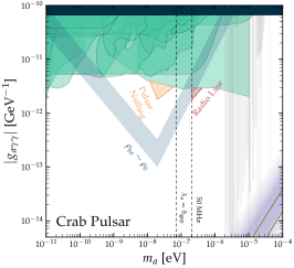
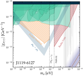
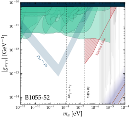
Figure 3: Same as Fig. 1, but showing the results for each of the three pulsars separately. Here, we also plot the the minimal coupling at which the projected axion density reaches $\epsilon_{\rm br}$ – this is shown as a blue band, with the width of the band reflecting the impact of varying $\xi\in[0.1,1]$. Vertical lines are drawn in each plot to indicate where $\lambda_{a}=h_{\rm gap}$ (above these curves we truncate the pulsar nulling contours) and the mass corresponding to $50$ MHz (below which we truncate the radio emission curves). Fig. 1 is the culmination of the bounds from all three of the shown pulsars.

Appendix E Magneto-rotational Spin-down

We have assumed throughout this work that the pulsar properties today are reflective of those earlier in its lifetime – this assumption is implicit in the linear scaling of the density profile with time. Neutron stars, however, are expected to undergo magneto-rotational spin-down, a process which can reduce the surface magnetic field strength and reduce the rotational frequency on timescales which are potentially shorter than the lifetime of the pulsars considered in this work. Here, we provide a very brief look at the impact of our current approximation.

The evolution of the pulsar period is determined by a combination of dipole radiation and plasma effects (see e.g. [92, 93]), and is described by the following equation:

$$\dot{P} = \beta\frac{B^{2}}{P}\,(\kappa_{0}+\kappa_{1}\sin^{2}\chi)\,.$$ (45)

The scenario in which $\kappa_{0}=0,\kappa_{1}=2/3$ corresponds to the case of pure dipole radiation, while $\kappa_{0}\sim\kappa_{1}\sim 1$ has been inferred from numerical simulations of plasma-filled magnetospheres [92, 93]. Eq. 45 is often complemented by those governing the decay of the magnetic field and the evolution of the misalignment angle. The evolution of both of these quantities, however, is highly uncertain, and thus in what follows we choose to treat both of these quantities as constant over the course of the neutron star lifetime. We expect this treatment to be conservative, as our choice amounts to an underestimation of the magnetic field and rotational frequency early in the life of the pulsar (the production rate being directly correlated with both of these quantities). The scenario in which $\kappa_{0}=0,\kappa_{1}=2/3$ corresponds to the case of pure dipole radiation, while $\kappa_{0}\sim\kappa_{1}\sim 1$ has been inferred from numerical simulations of plasma-filled magnetospheres [92, 93]. Eq. 45 is often complemented by those governing the decay of the magnetic field and the evolution of the misalignment angle. The evolution of both of these quantities, however, is highly uncertain, and thus in what follows we choose to treat both of these quantities as constant over the course of the neutron star lifetime. We expect this treatment to be conservative, as our choice amounts to an underestimation of the magnetic field and rotational frequency early in the life of the pulsar (the production rate being directly correlated with both of these quantities).

By evolving Eq. 45 backward from the current pulsar parameters, one can look the evolution of the axion production over the history of the neutron star lifetime. For simplicity, we adopt the coefficients $\kappa_{i}$ corresponding to the vacuum scenario, and take the initial magnetic alignment angles for the Crab, B1055-52, and J119-6127 corresponding to $\chi\sim 40^{\circ}$, $\chi\sim 85^{\circ}$, and $\chi\sim 5^{\circ}$, respectively [94, 96].

Having reconstructed $\Omega(t)$ for each pulsar, we follow the evolution of the density profile by replacing the linear time dependence of Eq. 3 with an integration. We find that in general, the axion surface density density obtained using this procedure tends to be greater than the linear approximation given in Eq. 3 by a an $\mathcal{O}(1)$ factor, making the linear extrapolation conservative.

Appendix F Sensitivity Analysis

Here, we outline the details of the sensitivity analysis leading to the projected contours shown in Fig. 1. We focus in particular on three pulsars, including the Crab pulsar (chosen as the prototypical example of a young pulsar which has been studied for more than half a century), J1119-6127 (a pulsar near the Galactic Center that was chosen because it produces a larger ratio of $\epsilon_{\rm sat}/\epsilon_{\rm br}$), and a nearby pulsar B1055-52 (chosen so as to maximize Eq. III). The details of each pulsar are included in Table 1.

Name / Property	Period [$s$]	$B_{0}$ [G]	$t_{\rm age}$ [yr]	d [kpc]	$S_{150}$	$S_{600}$	$S_{728}$	$S_{800}$	$S_{900}$	$S_{1382}$	$S_{3000}$
Crab	0.033	3.8e12	1e3	2	7500 [3800]	211 [37]	-	-	45 [10]	-	-
J1119-6127	0.407	4.1e13	1.6e3	8.4	-	-	3 [0.4]	-	-	1.09 [0.06]	0.36 [0.03]
B1055-52	0.197	1.09e12	5.3e5	0.093	310 [10]	-	22 [5]	20 [2]	-	4.4 [0.6]	1.4 [0.3]

Table 1: Properties of pulsars studied in this work. All flux densities are quoted in mJy, with $1\sigma$ uncertainties listed in brackets and the corresponding frequency in MHz given as lower labels (data is obtained from [97, 98, 99, 100]).

In order to determine the projected sensitivity to pulsar nulling, we determine the value of the axion photon coupling for which $\epsilon_{\rm br}(g_{a\gamma\gamma})=\epsilon_{\rm sat}$ and $\epsilon_{0}(g_{a\gamma\gamma})\geq\epsilon_{\rm br}(g_{a\gamma\gamma})$, i.e. we require the production of axions be sufficiently large to reach the back reaction density, and we require the back-reaction density be less than the saturation density. We only derive the back-reaction constraints for axion masses $m_{a}\leq 2\pi/h_{\rm gap}$, as it is unclear whether pulsar nulling will occur at higher masses. The derived limit is shown for each of the pulsars in the sample in Fig. 3, and is derived assuming that $\xi=0.1$ – taking a larger value of $\xi$ increases $\epsilon_{\rm br}\propto\xi^{2}$, and thus can reduce the projected sensitivity. As expected, J119-6127 shows the strongest projected sensitivity to pulsar nulling. The broken power law feature seen in the pulsar nulling limit of J119-6127 is a consequence of the fact that the de Broglie wavelength of the axion becomes larger than the radial size of the gap, and thus the induced electric field (and consequently the energy dissipation rate) becomes increasingly suppressed.

In order to determine the projected sensitivity to the radio line we must first estimate the expected background from the pulsar’s intrinsic flux. Table 1 contains the observed flux density (along with corresponding $1\sigma$ uncertainties) for each of the pulsars in the sample at a variety of frequencies. Our procedure for determining the background-subtracted sensitivity for each pulsar is as follows. First, for each frequency bin we randomly draw $\mathcal{O}(10^{3})$ samples about the mean observed value and taking the standard deviation to be the $1\sigma$ uncertainty. For each set of samples (defined as containing a single random draw at each of the observed frequencies), we perform a power law fit to the flux density, i.e. $S_{\nu}=A\times\,(\nu/1.4\,{\rm GHz})^{\alpha}$, and then evaluate the fit at the frequency of interest $\nu_{a}$. The collection of the samples $(S_{\nu,1}(\nu_{a}),\cdots,S_{\nu,N}(\nu_{a}))$ represent estimates of the pulsar spectrum at that frequency. We assume the uncertainty is characterized by the standard deviation $\sigma_{\nu}$ across all of the samples, and define our observable flux density threshold to be $2\times\sigma_{\nu}$ (note that we set an absolute lower limit on the threshold using the minimal error recorded in Table 1). We also impose an additional cut such that we only consider frequencies above 50 MHz, as lower frequencies can be efficiently absorbed before reaching Earth. The results are plotted for each pulsar in Fig. 3. Recall that B1055-22 has been selected to maximize the flux density in Eq. III; in Fig. 3 we see that the sensitivity is actually comparable to that of J119-6127 – this arises because Eq. III is only valid for axion-photon couplings above $g_{a\gamma\gamma}^{\rm min}$ (with the flux density scaling like $g_{a\gamma\gamma}^{4}$ for smaller couplings), and $g_{a\gamma\gamma}^{\rm min}$ for B1055-22 is larger than that of J1119-6127.

Appendix G An Aside on Resonant Transitions

One may wonder whether the growth of the background plasma can trigger resonant axion-photon transitions. Here, we argue that the level crossing generated during the growth of the pair plasma is expected to proceed sufficiently fast that conventional calculations of the resonant conversion probability break down. In this regime the conversion is expected to be heavily suppressed, however without a more detailed formalism it is difficult to make detailed calculations which compare the energy losses with the non-resonant production of photons.

In the non-relativistic limit, resonant axion-photon transitions occur when $m_{a}\simeq\omega_{p,{\rm eff}}$ where we have introduced the effective plasma frequency as the plasma frequency averaged over the inverse boost factor cubed, i.e. $\omega_{p,{\rm eff}}\equiv\left<\omega_{p}/\gamma^{3/2}\right>$. The probability of axion photon transitions is roughly given by (neglecting order-one angular pre-factors) $p_{a\rightarrow\gamma}\sim g_{a\gamma\gamma}^{2}\,B^{2}\,(\partial_{t}\omega_{p,{\rm eff}})^{-1}/v$. Note that the resonant timescale is roughly given by $t_{\rm res}\sim\sqrt{(\partial_{t}\omega_{p,{\rm eff}})^{-1}}$. The validity of the expressions outlined above are limited to the case where the background varies sufficiently slowly and level crossing is approximately linear in time.

In the gap, the effective plasma frequency is expected to grow from an initially small value, $\omega_{p,{\rm eff}}\sim\omega_{GJ,0}/(10^{6})^{3}$, to the GJ value at the pole $\omega_{GJ,0}$ (here, we have adopted a characteristic boost factor of $\gamma\sim 10^{6}$, with reasonable variations in this choice leading to negligible differences). The plasma is expected to grow exponentially, since plasma production proceeds iterativly over multiple generations with a growing multiplicity (and reduced boost factor) at each generation. Taking as an example an axion mass of $m_{a}\sim 10^{-6}$ eV, we find $t_{\rm res}$ to be much less than the oscillation timescale of the axion itself, illustrating that the conventional treatments of resonant mixing are invalid.

We leave a more detailed understanding of whether resonant transitions could contribute to additional photon production to future work, and simply note here that if resonances are capable of enhancing photon production (beyond what is generated non-resonantly), the dominant effect will be an enhancement the radio flux, which would imply that the treatment outlined here is conservative.

References

- [1] R. D. Peccei and H. R. Quinn, CP conservation in the presence of instantons, Phys. Rev. Lett. 38 (1977) 1440.
- [2] R. D. Peccei and H. R. Quinn, Constraints Imposed by CP Conservation in the Presence of Instantons, Phys. Rev. D16 (1977) 1791.
- [3] S. Weinberg, A new light boson?, Phys. Rev. Lett. 40 (1978) 223.
- [4] F. Wilczek, Problem of strong and invariance in the presence of instantons, Phys. Rev. Lett. 40 (1978) 279.
- [5] J. Preskill, M. B. Wise and F. Wilczek, Cosmology of the invisible axion, Phys. Lett. B 120 (1983) 127.
- [6] M. Dine and W. Fischler, The Not So Harmless Axion, Phys. Lett. B 120 (1983) 137.
- [7] A. Arvanitaki, S. Dimopoulos, S. Dubovsky, N. Kaloper and J. March-Russell, String axiverse, Phys. Rev. D 81 (2010) 123530 [0905.4720].
- [8] E. Witten, Some Properties of O(32) Superstrings, Phys. Lett. B 149 (1984) 351.
- [9] M. Cicoli, M. Goodsell and A. Ringwald, The type IIB string axiverse and its low-energy phenomenology, JHEP 10 (2012) 146 [1206.0819].
- [10] J. P. Conlon, The QCD axion and moduli stabilisation, JHEP 05 (2006) 078 [hep-th/0602233].
- [11] P. Svrcek and E. Witten, Axions In String Theory, JHEP 06 (2006) 051 [hep-th/0605206].
- [12] I. G. Irastorza and J. Redondo, New experimental approaches in the search for axion-like particles, Prog. Part. Nucl. Phys. 102 (2018) 89 [1801.08127].
- [13] M. S. Pshirkov and S. B. Popov, Conversion of Dark matter axions to photons in magnetospheres of neutron stars, J. Exp. Theor. Phys. 108 (2009) 384 [0711.1264].
- [14] A. Hook, Y. Kahn, B. R. Safdi and Z. Sun, Radio Signals from Axion Dark Matter Conversion in Neutron Star Magnetospheres, Phys. Rev. Lett. 121 (2018) 241102 [1804.03145].
- [15] G.-y. Huang, T. Ohlsson and S. Zhou, Observational Constraints on Secret Neutrino Interactions from Big Bang Nucleosynthesis, Phys. Rev. D97 (2018) 075009 [1712.04792].
- [16] M. Leroy, M. Chianese, T. D. P. Edwards and C. Weniger, Radio Signal of Axion-Photon Conversion in Neutron Stars: A Ray Tracing Analysis, Phys. Rev. D 101 (2020) 123003 [1912.08815].
- [17] B. R. Safdi, Z. Sun and A. Y. Chen, Detecting Axion Dark Matter with Radio Lines from Neutron Star Populations, Phys. Rev. D 99 (2019) 123021 [1811.01020].
- [18] R. A. Battye, B. Garbrecht, J. I. McDonald, F. Pace and S. Srinivasan, Dark matter axion detection in the radio/mm-waveband, Phys. Rev. D 102 (2020) 023504 [1910.11907].
- [19] J. W. Foster et al., Green Bank and Effelsberg Radio Telescope Searches for Axion Dark Matter Conversion in Neutron Star Magnetospheres, Phys. Rev. Lett. 125 (2020) 171301 [2004.00011].
- [20] J. W. Foster, S. J. Witte, M. Lawson, T. Linden, V. Gajjar, C. Weniger and B. R. Safdi, Extraterrestrial Axion Search with the Breakthrough Listen Galactic Center Survey, 2202.08274.
- [21] S. J. Witte, D. Noordhuis, T. D. Edwards and C. Weniger, Axion-photon conversion in neutron star magnetospheres: The role of the plasma in the Goldreich-Julian model, Physical Review D 104 (2021) .
- [22] A. J. Millar, S. Baum, M. Lawson and M. C. D. Marsh, Axion-photon conversion in strongly magnetised plasmas, JCAP 2021 (2021) 013 [2107.07399].
- [23] R. A. Battye, J. Darling, J. McDonald and S. Srinivasan, Towards robust constraints on axion dark matter using psr j1745-2900, 2021.
- [24] S. J. Witte, S. Baum, M. Lawson, M. C. D. Marsh, A. J. Millar and G. Salinas, Transient radio lines from axion miniclusters and axion stars, Phys. Rev. D 107 (2023) 063013 [2212.08079].
- [25] R. A. Battye, M. J. Keith, J. I. McDonald, S. Srinivasan, B. W. Stappers and P. Weltevrede, Searching for Time-Dependent Axion Dark Matter Signals in Pulsars, 2303.11792.
- [26] J. Tjemsland, J. McDonald and S. J. Witte, Adiabatic Axion-Photon Mixing Near Neutron Stars, 2310.18403.
- [27] A. Prabhu, Axion production in pulsar magnetosphere gaps, Phys. Rev. D 104 (2021) 055038 [2104.14569].
- [28] D. Noordhuis, A. Prabhu, S. J. Witte, A. Y. Chen, F. Cruz and C. Weniger, Novel Constraints on Axions Produced in Pulsar Polar Cap Cascades, 2209.09917.
- [29] D. Noordhuis, A. Prabhu, C. Weniger and S. J. Witte, Axion Clouds around Neutron Stars, 2307.11811.
- [30] A. Iwazaki, Axion stars and fast radio bursts, Phys. Rev. D 91 (2015) 023008 [1410.4323].
- [31] Y. Bai and Y. Hamada, Detecting Axion Stars with Radio Telescopes, Phys. Lett. B 781 (2018) 187 [1709.10516].
- [32] T. Dietrich, F. Day, K. Clough, M. Coughlin and J. Niemeyer, Neutron star–axion star collisions in the light of multimessenger astronomy, Mon. Not. Roy. Astron. Soc. 483 (2019) 908 [1808.04746].
- [33] A. Prabhu and N. M. Rapidis, Resonant Conversion of Dark Matter Oscillons in Pulsar Magnetospheres, JCAP 10 (2020) 054 [2005.03700].
- [34] T. D. P. Edwards, B. J. Kavanagh, L. Visinelli and C. Weniger, Transient Radio Signatures from Neutron Star Encounters with QCD Axion Miniclusters, Phys. Rev. Lett. 127 (2021) 131103 [2011.05378].
- [35] J. H. Buckley, P. S. B. Dev, F. Ferrer and F. P. Huang, Fast radio bursts from axion stars moving through pulsar magnetospheres, Phys. Rev. D 103 (2021) 043015 [2004.06486].
- [36] S. Nurmi, E. D. Schiappacasse and T. T. Yanagida, Radio signatures from encounters between Neutron Stars and QCD-Axion Minihalos around Primordial Black Holes, 2102.05680.
- [37] Y. Bai, X. Du and Y. Hamada, Diluted axion star collisions with neutron stars, JCAP 01 (2022) 041 [2109.01222].
- [38] A. Prabhu, Axion-mediated Transport of Fast Radio Bursts Originating in Inner Magnetospheres of Magnetars, Astrophys. J. Lett. 946 (2023) L52 [2302.11645].
- [39] M. C. Miller et al., PSR J0030+0451 Mass and Radius from Data and Implications for the Properties of Neutron Star Matter, Astrophys. J. Lett. 887 (2019) L24 [1912.05705].
- [40] M. C. Miller et al., The Radius of PSR J0740+6620 from NICER and XMM-Newton Data, Astrophys. J. Lett. 918 (2021) L28 [2105.06979].
- [41] D. Wouters and P. Brun, Constraints on Axion-like Particles from X-Ray Observations of the Hydra Galaxy Cluster, Astrophys. J. 772 (2013) 44 [1304.0989].
- [42] H.E.S.S. Collaboration, A. Abramowski et al., Constraints on axionlike particles with H.E.S.S. from the irregularity of the PKS 2155-304 energy spectrum, Phys. Rev. D 88 (2013) 102003 [1311.3148].
- [43] A. Payez et al., Revisiting the SN1987a gamma-ray limit on ultralight axion-like particles, Journal of Cosmology and Astroparticle Physics 2015 (2015) 006.
- [44] Fermi-LAT Collaboration, M. Ajello et al., Search for Spectral Irregularities due to Photon–Axionlike-Particle Oscillations with the Fermi Large Area Telescope, Phys. Rev. Lett. 116 (2016) 161101 [1603.06978].
- [45] M. Meyer, M. Giannotti, A. Mirizzi, J. Conrad and M. A. Sánchez-Conde, Fermi Large Area Telescope as a Galactic Supernovae Axionscope, Phys. Rev. Lett. 118 (2017) 011103 [1609.02350].
- [46] M. C. D. Marsh, H. R. Russell, A. C. Fabian, B. P. McNamara, P. Nulsen and C. S. Reynolds, A New Bound on Axion-Like Particles, JCAP 12 (2017) 036 [1703.07354].
- [47] C. S. Reynolds, M. C. D. Marsh, H. R. Russell, A. C. Fabian, R. Smith, F. Tombesi and S. Veilleux, Astrophysical limits on very light axion-like particles from Chandra grating spectroscopy of NGC 1275, Astrophys. J. 890 (2020) 59 [1907.05475].
- [48] M. Xiao, K. M. Perez, M. Giannotti, O. Straniero, A. Mirizzi, B. W. Grefenstette, B. M. Roach and M. Nynka, Constraints on Axionlike Particles from a Hard X-Ray Observation of Betelgeuse, Phys. Rev. Lett. 126 (2021) 031101 [2009.09059].
- [49] H.-J. Li, J.-G. Guo, X.-J. Bi, S.-J. Lin and P.-F. Yin, Limits on axion-like particles from Mrk 421 with 4.5-year period observations by ARGO-YBJ and Fermi-LAT, Phys. Rev. D 103 (2021) 083003 [2008.09464].
- [50] C. Dessert, J. W. Foster and B. R. Safdi, X-ray Searches for Axions from Super Star Clusters, Phys. Rev. Lett. 125 (2020) 261102 [2008.03305].
- [51] C. Dessert, A. J. Long and B. R. Safdi, No evidence for axions from chandra observation of the magnetic white dwarf RE j0317-853, Physical Review Letters 128 (2022) .
- [52] C. Dessert, D. Dunsky and B. R. Safdi, Upper limit on the axion-photon coupling from magnetic white dwarf polarization, Physical Review D 105 (2022) .
- [53] CAST Collaboration, V. Anastassopoulos et al., New cast limit on the axion–photon interaction, Nature Physics 13 (2017) 584–590.
- [54] P. Sikivie, Experimental tests of the ”invisible” axion, Phys. Rev. Lett. 51 (1983) 1415.
- [55] S. DePanfilis, A. Melissinos, B. Moskowitz, J. Rogers, Y. K. Semertzidis, W. Wuensch, H. Halama, A. Prodell, W. Fowler and F. Nezrick, Limits on the abundance and coupling of cosmic axions at 4.5¡ m a¡ 5.0 ev, Physical Review Letters 59 (1987) 839.
- [56] C. Hagmann, P. Sikivie, N. S. Sullivan and D. B. Tanner, Results from a search for cosmic axions, Phys. Rev. D 42 (1990) 1297.
- [57] ADMX Collaboration, C. Hagmann et al., Results from a high sensitivity search for cosmic axions, Phys. Rev. Lett. 80 (1998) 2043 [astro-ph/9801286].
- [58] ADMX Collaboration, S. J. Asztalos et al., Large scale microwave cavity search for dark matter axions, Phys. Rev. D 64 (2001) 092003.
- [59] ADMX Collaboration, S. J. Asztalos et al., A SQUID-based microwave cavity search for dark-matter axions, Phys. Rev. Lett. 104 (2010) 041301 [0910.5914].
- [60] ADMX Collaboration, N. Du et al., A Search for Invisible Axion Dark Matter with the Axion Dark Matter Experiment, Phys. Rev. Lett. 120 (2018) 151301 [1804.05750].
- [61] ADMX Collaboration, T. Braine et al., Extended search for the invisible axion with the axion dark matter experiment, Physical Review Letters 124 (2020) .
- [62] R. Bradley et al., Microwave cavity searches for dark-matter axions, Rev. Mod. Phys. 75 (2003) 777.
- [63] S. J. Asztalos et al., Improved rf cavity search for halo axions, Phys. Rev. D 69 (2004) 011101.
- [64] T. M. Shokair et al., Future directions in the microwave cavity search for dark matter axions, International Journal of Modern Physics A 29 (2014) 1443004.
- [65] HAYSTAC Collaboration, B. M. Brubaker et al., First results from a microwave cavity axion search at , Phys. Rev. Lett. 118 (2017) 061302.
- [66] HAYSTAC Collaboration, L. Zhong et al., Results from phase 1 of the haystac microwave cavity axion experiment, Physical Review D 97 (2018) .
- [67] HAYSTAC Collaboration, K. M. Backes et al., A quantum enhanced search for dark matter axions, Nature 590 (2021) 238.
- [68] B. T. McAllister et al., The organ experiment: An axion haloscope above 15 ghz, 2017.
- [69] QUAX Collaboration, N. Crescini et al., Axion search with a quantum-limited ferromagnetic haloscope, Phys. Rev. Lett. 124 (2020) 171801 [2001.08940].
- [70] J. Choi, S. Ahn, B. R. Ko, S. Lee and Y. K. Semertzidis, CAPP-8TB: Axion dark matter search experiment around 6.7 ev, Nucl. Instrum. Meth. A 1013 (2021) 165667 [2007.07468].
- [71] CAST Collaboration, A. A. Melcón et al., First results of the CAST-RADES haloscope search for axions at 34.67 eV, JHEP 21 (2020) 075 [2104.13798].
- [72] M. A. Ruderman and P. G. Sutherland, Theory of pulsars: polar gaps, sparks, and coherent microwave radiation., Astrophys. J. 196 (1975) 51.
- [73] A. Timokhin, Time-dependent pair cascades in magnetospheres of neutron stars–i. dynamics of the polar cap cascade with no particle supply from the neutron star surface, Monthly Notices of the Royal Astronomical Society 408 (2010) 2092.
- [74] A. N. Timokhin and J. Arons, Current Flow and Pair Creation at Low Altitude in Rotation Powered Pulsars’ Force-Free Magnetospheres: Space-Charge Limited Flow, Mon. Not. Roy. Astron. Soc. 429 (2013) 20 [1206.5819].
- [75] A. Philippov, A. Timokhin and A. Spitkovsky, Origin of Pulsar Radio Emission, Phys. Rev. Lett. 124 (2020) 245101 [2001.02236].
- [76] P. Goldreich and W. H. Julian, Pulsar electrodynamics, Astrophys. J. 157 (1969) 869.
- [77] A. N. Timokhin and A. K. Harding, On the Polar Cap Cascade Pair Multiplicity of Young Pulsars, Astrophys. J. 810 (2015) 144 [1504.02194].
- [78] A. N. Timokhin and A. K. Harding, On the maximum pair multiplicity of pulsar cascades, Astrophys. J. 871 (2019) 12 [1803.08924].
- [79] A. Philippov and M. Kramer, Pulsar Magnetospheres and Their Radiation, Annual Review of Astronomy and Astrophysics 60 (2022) 495.
- [80] A. G. Lyne, R. S. Pritchard and F. Graham Smith, 23 years of Crab pulsar rotational history., Monthly Notices of the Royal Astronomical Society 265 (1993) 1003.
- [81] A. Lyne, F. Graham-Smith, P. Weltevrede, C. Jordan, B. Stappers, C. Bassa and M. Kramer, Evolution of the Magnetic Field Structure of the Crab Pulsar, Science 342 (2013) 598 [1311.0408].
- [82] S. E. Gralla, A. Lupsasca and A. Philippov, Inclined Pulsar Magnetospheres in General Relativity: Polar Caps for the Dipole, Quadrudipole and Beyond, Astrophys. J. 851 (2017) 137 [1704.05062].
- [83] F. Wilczek, Two Applications of Axion Electrodynamics, Phys. Rev. Lett. 58 (1987) 1799.
- [84] Arons, Jonathan and Barnard, John J, Wave propagation in pulsar magnetospheres-Dispersion relations and normal modes of plasmas in superstrong magnetic fields, Astrophysical Journal 302 (1986) 120.
- [85] F. Cruz, T. Grismayer, A. Y. Chen, A. Spitkovsky and L. O. Silva, Coherent emission from QED cascades in pulsar polar caps, 2108.11702.
- [86] M. Beutter, A. Pargner, T. Schwetz and E. Todarello, Axion-electrodynamics: a quantum field calculation, JCAP 02 (2019) 026 [1812.05487].
- [87] J. D. Jackson, Classical Electrodynamics. Wiley, 1998.
- [88] G. G. Raffelt, Stars as Laboratories for Fundamental Physics. University of Chicago Press, 1996.
- [89] A. Caputo, S. J. Witte, D. Blas and P. Pani, Electromagnetic signatures of dark photon superradiance, Phys. Rev. D 104 (2021) 043006 [2102.11280].
- [90] A. K. Harding and A. G. Muslimov, Particle acceleration zones above pulsar polar caps: electron and positron pair formation fronts, The Astrophysical Journal 508 (1998) 328.
- [91] E. A. Tolman, A. A. Philippov and A. N. Timokhin, Electric Field Screening in Pair Discharges and Generation of Pulsar Radio Emission, Astrophys. J. Lett. 933 (2022) L37 [2202.01303].
- [92] A. Spitkovsky, Time-dependent force-free pulsar magnetospheres: Axisymmetric and oblique rotators, The Astrophysical Journal 648 (2006) L51.
- [93] A. Philippov, A. Tchekhovskoy and J. G. Li, Time evolution of pulsar obliquity angle from 3d simulations of magnetospheres, Monthly Notices of the Royal Astronomical Society 441 (2014) 1879.
- [94] A. Lyne, F. Graham-Smith, P. Weltevrede, C. Jordan, B. Stappers, C. Bassa and M. Kramer, Evolution of the magnetic field structure of the crab pulsar, Science 342 (2013) 598.
- [95] A. Lyne, C. Jordan, F. Graham-Smith, C. Espinoza, B. Stappers and P. Weltevrede, 45 years of rotation of the crab pulsar, Monthly Notices of the Royal Astronomical Society 446 (2015) 857.
- [96] S. Rookyard, P. Weltevrede and S. Johnston, Constraints on viewing geometries from radio observations of -ray-loud pulsars using a novel method, Monthly Notices of the Royal Astronomical Society 446 (2015) 3367.
- [97] F. Jankowski, M. Bailes, W. van Straten, E. Keane, C. Flynn, E. Barr, T. Bateman, S. Bhandari, M. Caleb, D. Campbell-Wilson et al., The utmost pulsar timing programme i: Overview and first results, Monthly Notices of the Royal Astronomical Society 484 (2019) 3691.
- [98] M. Bell, T. Murphy, S. Johnston, D. Kaplan, S. Croft, P. Hancock, J. Callingham, A. Zic, D. Dobie, J. Swiggum et al., Time-domain and spectral properties of pulsars at 154 mhz, Monthly Notices of the Royal Astronomical Society 461 (2016) 908.
- [99] F. Jankowski, W. Van Straten, E. Keane, M. Bailes, E. Barr, S. Johnston and M. Kerr, Spectral properties of 441 radio pulsars, Monthly Notices of the Royal Astronomical Society 473 (2018) 4436.
- [100] P. Weltevrede, S. Johnston and C. M. Espinoza, The glitch-induced identity changes of psr j1119- 6127, Monthly Notices of the Royal Astronomical Society 411 (2011) 1917.