Fluctuation corrections to Lifshitz tails in disordered systems

Abstract

Quenched disorder in semiconductors induces localized electronic states at the band edge, which manifest as an exponential tail in the density of states. For large impurity densities, this tail takes a universal Lifshitz form that is characterized by short-ranged potential fluctuations. We provide both analytical expressions and numerical values for the Lifshitz tail of a parabolic conduction band, including its exact fluctuation prefactor. Our analysis is based on a replica field integral approach, where the leading exponential scaling of the tail is determined by an instanton profile, and fluctuations around the instanton determine the subleading pre-exponential factor. This factor contains the determinant of a fluctuation operator, and we avoid a full computation of its spectrum by using a Gel’fand-Yaglom formalism, which provides a concise general derivation of fluctuation corrections in disorder problems. We provide a revised result for the disorder band tail in two dimensions.

Disorder is an inherent property of physical systems, arising, for example, as defects or impurities in doped semiconductors [1], frozen non-equilibrium degrees of freedom in quenched alloys and glasses [2, 3], or thermal fluctuations [4]. It can also be engineered in photonic structures [5, 6] or quantum gases in an optical speckle potential [7, 8]. For the electronic density of states in a semiconductor, disorder has two effects: First, it induces a narrowing of the band gap, where valence and conduction band levels are raised and lowered, respectively, by a characteristic impurity energy. Second, it causes band tailing, where fluctuations in the disorder potential give rise to localized states inside the band gap. Describing the disorder-induced band narrowing and tailing is important because it affects semiconductor devices like transistors [9, 1, 10] or limits the efficiency of solar cells [11, 12], and it sets the variable-range hopping conduction that dominates transport in localized systems at low temperatures [13].

In general, potential fluctuations large enough to generate states with energies far away from the band edge are rare, and the tail of localized levels takes an exponential form (written here for a single conduction band) [14, 15, 16, 1],

$$\langle\rho(E)\rangle\overset{E\to-\infty}{=}A(E)e^{-B(E)},$$ (1)

where $E$ is the energy below the band edge and $\langle\cdot\rangle$ denotes a disorder average. Of particular interest is the limit of high impurity density, which is universal in the sense that, over a large energy range, the band tail is insensitive to details of the disorder correlations [1]. This is the Lifshitz region or Lifshitz tail [17, 18], where (1) takes a stretched exponential form. Remarkably, even for the seemingly simple case of noninteracting particles in a Gaussian-correlated disorder potential, the disorder-averaged density of states can only be computed exactly in one dimension (1D) [19]. In higher dimensions, dating back to works by Halperin and Lax [19, 20, 21] and Zittartz and Langer [22], the tail exponential $B(E)$ is obtained from a variational argument that determines the most likely disorder potential giving rise to a bound state at large negative energy $E$. Such variational arguments are quite general and may be extended to include the effect of correlated disorder [23], magnetic fields [24], interactions [25], and also to describe the spectra of random operators [26, 27, 28]. However, they do not capture the prefactor $A(E)$ in the density of states (1), which is set by fluctuations of the disorder potential and requires the evaluation of a functional determinant. The established result for $A(E)$ derived by Brézin and Parisi [29] is based on an analysis of large-order perturbations in $\phi^{4}$ theory discussed in a classical paper by the same authors [30], which evaluates the fluctuation determinant by exact diagonalization [31, 30]. At the same time, the computation of fluctuation corrections is a common problem, for example to determine the decay rate of metastable states [32]. Indeed, one of the first studies on the subject by Gel’fand and Yaglom [33], Levit and Smilansky [34] in the context of one-dimensional path integrals in quantum mechanics avoids the direct evaluation of the fluctuation spectrum by mapping the functional determinant to a differential equation, a much simpler problem. Intriguingly, such an approach has also been applied to higher-dimensional problems [35], which suggests that an efficient computation of the fluctuation prefactor $A(E)$ should exist.

In this Letter, we show that this is indeed the case and compute the prefactor $A(E)$ of the Lifshitz tail (1) without evaluating the full fluctuation determinant, which in particular provides a revised result for the band tail in two dimensions. While the calculation is very general, we focus on the universal Lifshitz regime of infinitely dense but infinitesimally weak point scatterers, which is described by a Gaussian white noise disorder potential,

$$\langle V(\bm{x})\rangle=0,\quad\langle V(\bm{x})V(\bm{x^{\prime}})\rangle=w^{2}\delta(\bm{x}-\bm{x^{\prime}}),$$ (2)

and consider a parabolic conduction band described by the one-electron Hamiltonian

$$H^{V}=-\frac{\hbar^{2}}{2m}\nabla^{2}+V(\bm{x}).$$ (3)

Throughout the paper, we set $\hbar=2m=1$. We base our calculation on a functional integral representation for the disorder-averaged density of states, which we evaluate in a saddle-point approximation including fluctuations. The central results of our work are the following revised expressions for the density of states in the deep-tail regime (i.e., for $E\to-\infty$):

$$\frac{\langle\rho(E)\rangle}{\rho_{0}(-E)}\overset{E\to-\infty}{=}\begin{cases}\dfrac{8|E|^{3/2}}{w^{2}}e^{-\frac{8|E|^{3/2}}{3w^{2}}}&d=1\\[12.91663pt] 20.06~{}\dfrac{|E|^{3/2}}{w^{3}}e^{-11.70\frac{|E|}{w^{2}}}&d=2\\[12.91663pt] 8796\hskip 2.77779pt~{}\dfrac{|E|}{w^{4}}e^{-37.79\frac{|E|^{1/2}}{w^{2}}}&d=3,\end{cases}$$ (4)

expressed here in relation to the density of states of the free Hamiltonian, $\rho_{0}=E^{d/2-1}/(4\pi)^{d/2}\Gamma(d/2)$. The 1D and 3D cases agree with previous results derived using other means [19, 20, 29], but the 2D result corrects an existing literature value [29].

The starting point of our analysis is a functional integral representation of the disorder-averaged density of states

$$\begin{split}&\langle\rho(E)\rangle=\int\mathcal{D}[V]e^{-\int d\bm{x}\frac{V^{2}(\bm{x})}{2w^{2}}}\frac{1}{L^{d}}\sum_{n}\delta\left(E-E^{V}_{n}\right)\\ &=\frac{-i}{\pi L^{d}}\biggl{\langle}\frac{\partial}{\partial E}\bigl{[}\ln{\cal Z}^{V}(E+i0)-\ln{\cal Z}^{V}(E-i0)\bigr{]}\biggr{\rangle}.\end{split}$$ (5)

Here, the probability measure for the random field $V(\bm{x})$ is normalized to unity, $L^{d}$ is the $d$-dimensional volume, and $E^{V}_{n}$ is the $n$-th energy eigenvalue for a realization of the Hamiltonian (3) with potential $V(\bm{x})$. In the second line, we introduce the partition function

$$\begin{split}{\cal Z}^{V}(E)&=\prod_{n}\left(E_{n}^{V}-E\right)^{-1/2}\\ &=\int\mathcal{D}[\phi]\,\exp\left[-\frac{1}{2}\int d\bm{x}\,\phi\left(H^{V}-E\right)\phi\right],\end{split}$$ (6)

which we express as a path integral over a scalar field $\phi({\bf x})$. Written in this form, Eq. (5) is equivalent to the Edwards-Jones formula for the eigenvalue distribution of the random matrix $H^{V}$ [36, 37]. The factors $(E_{n}^{V}-E)^{-1/2}$ in the partition function have a branch cut for $E>E^{V}_{n}$, resulting in a discontinuity between complex energies $E\pm i0$, and thus a nonzero contribution to the density of states (5). The analytic continuation of the path integral to energies $E\pm{}i0$ is performed by rotating the fields $\phi$ in Eq. (6) into the complex plane by an angle $e^{\pm i\pi/4}$, i.e., on a contour $C^{\pm}$ along the positive and negative complex diagonals [38, 39, 40, 32].

The disorder average (5) is difficult to compute directly due to the presence of the logarithm; therefore, we apply the replica trick [41], $\ln\mathcal{Z}=\lim_{N\to 0}(\mathcal{Z}^{N}-1)/N$, which avoids the logarithm in favor of introducing $N$ copies (replicas) of the original system. The disorder average is now performed exactly as a Gaussian integral over the potential $V(\bm{r})$, which gives

$$\langle\rho(E)\rangle=\lim_{N\to 0}\frac{(-E)^{1-\frac{d}{2}}}{i\pi w^{2}NL^{d}}\int_{C^{+}-C^{-}}\mathcal{D}[\Phi]\int d\bm{r}\,\Phi^{2}e^{-\frac{1}{g}S[\Phi]},$$ (7)

where the subscript indicates that we consider the difference over both contours, $\Phi(\bm{r})=\sqrt{-w^{2}/2E}\,(\phi_{1},\dots,\phi_{N})$ is a vector of dimensionless replica fields that depend on a dimensionless position ${\bm{r}}={\bm{x}}\sqrt{-E}$, and we introduce the scaling parameter

$$\frac{1}{g}=\frac{(-E)^{2-\frac{d}{2}}}{w^{2}}.$$ (8)

The effective action

$$S[\Phi]=\int d\bm{r}~{}\Phi\biggl{(}-\nabla^{2}+1-\frac{1}{2}\Phi^{2}\biggr{)}\Phi$$ (9)

corresponds to a $\phi^{4}$ Ginzburg-Landau theory [39], where the disorder field is removed at the expense of introducing a nonlinear term. Crucially, for $d<4$, the prefactor $g^{-1}$ of the effective action (7) is large in the deep-tail regime, $E\to-\infty$. This allows us to evaluate the integral over the replica field $\Phi$ in the saddle-point approximation [42], that is, by expanding around the dominant contribution to the action.

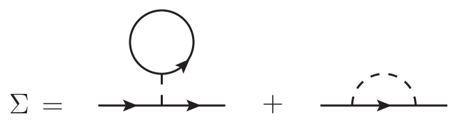
Figure 1: Divergent self-energy diagrams for the $\phi^{4}$ theory (9).

Before evaluating the saddle-point, however, note that the theory (9) requires renormalization. The divergent one-loop self-energy corrections are shown in Fig. 1, where a continuous line denotes the free Green’s function and the vertex is split to connect two replica indices. Physically, the divergences are a consequence of the white-noise approximation (2) to the disorder potential, which breaks down as the field $\Phi$ varies over length scales smaller than the separation between scatterers. The divergences are subtracted by adding a counterterm to the action (9),

$$\delta S[\Phi]=\frac{N+2}{2}g\,G_{0}\int d\bm{r}\,\Phi^{2},$$ (10)

which is linear in $g$ and will thus give a subleading correction in the saddle-point approximation. Here,

$$G_{0}=\int\frac{d\bm{q}}{(2\pi)^{d}}\,\frac{1}{q^{2}+1}$$ (11)

is the free Green’s function at coinciding points, which diverges in $d\geq 2$, and the factor $N+2$ in Eq. (10) arises from the different contractions of the replica fields. The self-energy $\Sigma(E)$ computed including the counterterm is finite and represents the band narrowing that shifts the reference point $E_{0}$ of the energy scale. Including the finite part of $G_{0}$ in the counterterm corresponds to a renormalization choice $\Sigma(E)|_{0}=0$ that puts this reference at the origin [43]. Another possible choice is $\partial\Sigma(E)/\partial E|_{0}=1$, which is motivated from a coherent potential approximation [29, 44]. Results computed in different schemes are identical and linked by a shift in the energy parameter (with possible logarithmic corrections in 2D).

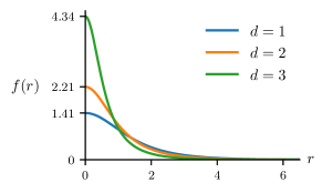
Figure 2: Instanton solution of the saddle-point equation (12), which determines the leading scaling of the band tail $B(E)$.

The leading saddle point of the action (9) is the trivial configuration $\Phi=0$; however, this contribution is the same for both contours $C^{\pm}$ and cancels when taking the difference in Eq. (7). The parameter $B(E)$ in the exponential band tail (1) is thus determined by the action at the subleading saddle point of Eq. (7), which is of order $S[\Phi]={\cal O}(g^{-1})$. The field configuration that minimizes the effective action (9) is of the form $\Phi(\bm{r}+\bm{r}_{0})=f(r)\,\bm{u}$ [45, 40], where $\bm{r}_{0}$ is an arbitrary center, $\bm{u}$ an arbitrary unit vector in replica space, and $f(r)$ is a nodeless radial function known as the instanton. The saddle-point equation is

$$-\nabla^{2}f(r)+f(r)-f^{3}(r)=0,$$ (12)

with boundary conditions $f^{\prime}(0)=f(r\to\infty)=0$. We can interpret it as a Schrödinger equation for the potential $-f^{2}(r)$ that describes the most likely shape of the disorder potential with a bound state at energy $E$ [25]. Figure 2 shows the instanton profile in $d=1,2$, and $3$. In 1D, the solution $f(r)=\sqrt{2}\,\text{sech}(r)$ is known analytically, and for $d\geq 2$, we employ a spectral renormalization method to solve Eq. (12) numerically [46]. The exponential band tail is then given by the saddle-point action

$$B(E)=\frac{1}{g}S[f]=\frac{I_{4}}{2g},$$ (13)

where

$$I_{n}=\int d\bm{r}\,f^{n}(r).$$ (14)

The corresponding values for $I_{4}$ are well established [31, 40] and tabulated in Tab. 1.

$d$	$1$	$2$	$3$
$I_{2}$	4	11.7009	18.8973
$I_{4}$	16/3	23.4018	75.5890
$e^{I_{2}G_{0}}D\left(1/3\right)$	1/4	1.0558	0.364
$e^{3I_{2}G_{0}}D(1)$	$-$1/12	$-$5.35	$-$0.0096

Table 1: Numerical values for the moments of the instanton profile (14) and for the normalized longitudinal and transverse fluctuation determinant $e^{3zI_{2}G_{0}}D(z)$ in $d=1$, $2$, and $3$.

Our main task in this paper is to determine the leading contribution to the prefactor $A(E)$ of the exponential band tail (1) by evaluating the next order in the saddle-point approximation. To this end, we expand the action to second order in new fields that represent longitudinal ($\delta f_{\parallel}$) and transverse ($\delta f_{\perp}^{k}$) fluctuations,

$$\Phi(\bm{r})=\bm{u}\left[f(r)+\delta f_{\parallel}(\bm{r})\right]+\sum_{k=1}^{N-1}\bm{v}_{k}\delta f_{\perp}^{k}(\bm{r}),$$ (15)

where the set $\{\bm{u},\bm{v}_{1},\dots,\bm{v}_{N-1}\}$ forms an orthonormal basis of replica space. However, certain fluctuations do not represent small corrections to the saddle-point action. These so-called zero modes correspond to changes of the orientation $\bm{u}$ of the instanton in replica space and of its center $\bm{r}_{0}$. These changes leave the action invariant and thus cannot be treated perturbatively, but must rather be integrated exactly. This is done using the method of collective coordinates [47], resulting in an overall factor

$$A_{0}=\left(\frac{I_{4}}{4\pi g}\right)^{\frac{d}{2}}\left[L\sqrt{-E}\right]^{d}\,\left(\frac{I_{2}}{\pi g}\right)^{\frac{N-1}{2}}\frac{2\pi^{N/2}}{\Gamma(N/2)}.$$ (16)

Here, terms in round brackets are the Jacobian of the transformation to the collective position $\bm{r}_{0}$ and angle coordinate $\bm{u}$. Note that this contribution introduces additional factors of $g$ and thus sets part of the energy dependence of the prefactor $A(E)$. The remaining terms correspond to the measure of the degenerate symmetry spaces, which is the $N$-dimensional surface element in replica space and the real-space volume $L^{d}$.

Formally, the full fluctuation correction reads

$$\begin{split}&A(E)=\lim_{N\to 0}\frac{(-E)^{1-\frac{d}{2}}}{i\pi w^{2}NL^{d}}I_{2}A_{0}\,e^{-\frac{N+2}{2}G_{0}I_{2}}\\[6.45831pt] &\times\int\mathcal{D}[\delta f]\,e^{-\frac{1}{g}\int d\bm{r}\left(\delta f_{\parallel}\Delta_{1}\delta f_{\parallel}+\sum_{k}\delta f_{\perp}^{k}\Delta_{1/3}\delta f_{\perp}^{k}\right)},\end{split}$$ (17)

where the factor $I_{2}$ is the saddle-point value of the field $\Phi^{2}$ in Eq. (7), the exponential prefactor is the counterterm contribution (10), and we define the fluctuation kernel

$$\Delta_{z}=-\nabla^{2}+1-3zf^{2},$$ (18)

which describes the decoupled longitudinal ($z=1$) and transverse ($z=1/3$) fluctuations. The excluded zero modes that correspond to an infinitesimal shift along one coordinate axis $\alpha=1,\ldots,d$ are linked to $d$ zero modes of the longitudinal fluctuation kernel $\Delta_{1}$ given by $\partial_{\alpha}f(\bm{r})$. Likewise, the operator $\Delta_{1/3}$ has a zero mode $f(\bm{r})$ corresponding to rotations in replica space. The path integral in Eq. (17) over the fluctuations $\delta f_{\parallel}$, $\delta f_{\perp,k}$ excludes the zero modes. It is then a Gaussian integral and results in factors involving the functional determinant of $\Delta_{z}$,

$$D(z)=\lim_{\varepsilon\to 0}\frac{1}{\varepsilon^{m}}\det\frac{\Delta_{z}+\varepsilon}{\Delta_{0}+\varepsilon},$$ (19)

where for the shifted operator $\Delta_{z}+\varepsilon$ the zero modes have eigenvalue $\varepsilon$, and are thus removed in the limit $\varepsilon\to 0$ ($m$ is the degeneracy of zero modes, with $m=d$ for $z=1$ and $m=1$ for $z=1/3$).

Taken together, the longitudinal and transverse fluctuation contribution to the path integral (17) reads

$$\begin{split}A(E)&=\lim_{N\to 0}\frac{(-E)^{1-\frac{d}{2}}}{\pi w^{2}NL^{d}}I_{2}A_{0}\\ &\qquad\times\Bigl{[}e^{3I_{2}G_{0}}\bigl{|}D(1)\bigr{|}\Bigr{]}^{-\frac{1}{2}}\Bigl{[}e^{I_{2}G_{0}}D\left(\tfrac{1}{3}\right)\Bigr{]}^{-\frac{N-1}{2}},\end{split}$$ (20)

where the exponent in the third factor accounts for the $N-1$ transverse replica field directions, and we split up the counterterm contribution. Note that the longitudinal kernel $D(1)$ is negative since it contains a single eigenfunction $f$ with negative eigenvalue $-2$. The square root is still well defined after analytic continuation, and the resulting imaginary unit cancels with that in the prefactor of Eq. (17). Moreover, in $d>1$, the fluctuation determinant $D(z)$ diverges. The mathematical origin of this divergence is identified by expanding the determinant in powers of $z$,

$$\text{det}\biggl{[}1-\frac{3zf^{2}}{-\nabla^{2}+1}\biggr{]}=e^{1-3zI_{2}G_{0}+\mathcal{O}(z^{2})},$$ (21)

where $G_{0}$ is introduced in Eq. (11) and higher-order terms in $z$ are finite. The divergent term in Eq. (21), however, is precisely canceled by the leading-order counterterm (10), rendering the fluctuation determinant (20) manifestly finite.

To evaluate the finite renormalized fluctuation determinant, one could in principle compute the eigenvalues of $\Delta_{z}$ and evaluate their product, which was done in a similar context by Brézin and Parisi [30] to determine the large-order behaviour of perturbation series in $\phi^{4}$ theories. Here, we make use of a more direct method using spectral functions. This method was originally proposed by Gel’fand and Yaglom [33], and applied to higher-dimensional problems with radial symmetry in [35] (for a review, see [48, 49, 50]). Crucially, the Gel’fand-Yaglom method does not require knowledge of the eigenvalues, but instead expresses the functional determinant in terms of the solution to an ordinary differential equation, which greatly simplifies the overall calculation.

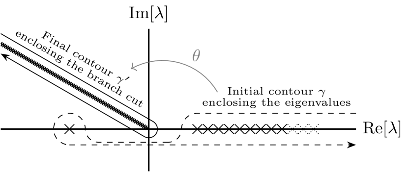
Figure 3: Complex structure of the integral (24). Crosses indicate eigenvalues (shown here for longitudinal fluctuations with one negative eigenvalue) and the wavy line denotes the branch cut. The dashed line indicates the initial integration contour $\gamma$ that encloses all eigenvalues, and the solid line shows the deformed contour $\gamma^{\prime}$ that runs around the branch cut.

The Gel’fand-Yaglom method is based on the formal identity [34]

$$\det\Delta_{z}=\prod_{n}\lambda_{n}=e^{-\zeta_{z}^{\prime}(0)},$$ (22)

where $\lambda_{n}$ are the eigenvalues of the operator $\Delta_{z}$, defined in Eq. (18), and

$$\zeta_{z}(s)=\sum_{n}\frac{1}{\lambda_{n}^{s}}.$$ (23)

We introduce an analytic function $\mathcal{F}_{z}(\lambda)$ with zeros that coincide in location and multiplicity with the eigenvalues $\lambda_{n}$, in terms of which

$$\begin{split}&\zeta_{z}(s)-\zeta_{0}(s)=\frac{1}{2\pi i}\int_{\gamma}d\lambda\,\lambda^{-s}\frac{d}{d\lambda}\left[\ln\frac{\mathcal{F}_{z}(\lambda)}{\mathcal{F}_{0}(\lambda)}\right]\\ &=e^{-is(\pi-\theta)}\frac{\sin\pi s}{\pi}\int_{0}^{\infty}d\lambda\,\lambda^{-s}\frac{d}{d\lambda}\left[\ln\frac{\mathcal{F}_{z}(e^{i\theta}\lambda)}{\mathcal{F}_{0}(e^{i\theta}\lambda)}\right].\end{split}$$ (24)

Here, the contour $\gamma$ encircles all eigenvalues, and we place the branch cut of the integrand at an angle $\theta$ with the real axis to avoid overlapping with the eigenvalues [48], see Fig. 3 for an illustration. To obtain the last identity, we deform the contour to enclose the branch cut, which is shown as a continuous line in Fig. 3. We may now take the derivative with respect to $s$ to obtain

$$\det\frac{\Delta_{z}}{\Delta_{0}}=e^{-\zeta_{z}^{\prime}(0)+\zeta_{0}^{\prime}(0)}=\frac{\mathcal{F}_{z}(0)}{\mathcal{F}_{0}(0)}=\prod_{l=0}^{\infty}\left[\frac{\mathcal{F}^{(l)}_{z}(0)}{\mathcal{F}^{(l)}_{0}(0)}\right]^{{\rm d}(l;d)},$$ (25)

where we use the rotational symmetry of $\Delta_{z}$ to factorize the determinant and by extension $\mathcal{F}$ into angular components $\mathcal{F}^{(l)}$ [35], and we denote the angular degeneracy of the eigenvalues by ${\rm d}(l;d)$. Note that in 1D the rotational symmetry reduces to a parity symmetry; thus, $l$ labels only nondegenerate even ($l=0$) and odd ($l=1$) contributions. Intuitively, the function $\mathcal{F}_{z}(\lambda)$ generalizes the characteristic polynomial of finite-dimensional matrices to the operator $\Delta_{z}$. Equation (25) then corresponds to the result that the constant term in the characteristic polynomial is the determinant.

To obtain $\mathcal{F}^{(l)}_{z}(\lambda)$, we follow the same heuristic as used to find eigenvalues numerically with the shooting method [48]: Consider the function $\phi^{(l)}_{z}(\lambda,r)$ obtained by solving the initial value problem

$$\left(\Delta^{(l)}_{z}+\varepsilon\right)\phi_{z}^{(l)}=\lambda\phi_{z}^{(l)},\quad\phi_{z}^{(l)}(\lambda,r)\overset{r\to 0}{\sim}r^{l+\frac{d-1}{2}},$$ (26)

where we include the factor $\varepsilon\ll 1$ in Eq. (19), and

$$\Delta^{(l)}_{z}=-\frac{d^{2}}{dr^{2}}+\frac{(l+\frac{d-3}{2})(l+\frac{d-1}{2})}{r^{2}}+1-3zf^{2}.$$ (27)

If $\lambda$ is such that the function vanishes at infinity, $\phi_{z}^{(l)}(\lambda,\infty)=0$, $\phi$ will also be an eigenfunction of $\Delta^{(l)}_{z}$ with eigenvalue $\lambda$. But this is exactly the defining property of $\mathcal{F}_{z}^{(l)}$, and hence we set $\mathcal{F}^{(l)}_{z}(\lambda)=\phi_{z}^{(l)}(\lambda,\infty)$. Note that only the ratio $\mathcal{R}_{z,\varepsilon}^{(l)}=\mathcal{F}_{z}^{(l)}/\mathcal{F}_{0}^{(l)}$ contributes to Eq. (25), so it is useful to derive an equation for $\mathcal{R}_{z,\varepsilon}^{(l)}$ directly [51]

$$\begin{split}&0=\mathcal{R}_{z,\varepsilon}^{(l)\prime\prime}(r)+3zf^{2}(r)\mathcal{R}_{z,\varepsilon}^{(l)}(r)\\ &+\left[\frac{2l+d-1}{r}+2\sqrt{1+\varepsilon}\frac{I_{l+\frac{d}{2}}\left(\sqrt{1+\varepsilon}r\right)}{I_{l+\frac{d}{2}-1}\left(\sqrt{1+\varepsilon}r\right)}\right]\mathcal{R}_{z,\varepsilon}^{(l)\prime}(r),\end{split}$$ (28)

with boundary conditions $\mathcal{R}_{z,\varepsilon}^{(l)}(0)=1$ and $\mathcal{R}_{z,\varepsilon}^{(l)\prime}(0)=0$, inherited from Eq. (26). Here, $I$ is the modified Bessel function of the first kind.

The renormalized determinant, finite to all orders in $z$ and without zero modes, reads

$$\begin{split}&\ln\bigl{[}e^{-zI_{2}G_{0}}D(z)\bigr{]}\\ &=\lim_{\varepsilon\to 0}\sum_{l=0}^{\infty}{\rm d}(l;d)\left[\frac{1}{\varepsilon^{\delta_{l}}}\ln\mathcal{R}^{(l)}_{z,\varepsilon}(\infty)-zr^{(l)}\right],\end{split}$$ (29)

where $\delta_{l}$ is equal to unity if $\Delta_{z}^{(l)}$ has a zero mode, and zero otherwise. The second term in the bracket is the counterterm contribution, which in our discussion of Eq. (21) we identified as the term of linear order in $z$, and which is thus written as

$$\begin{split}r^{(l)}&=\frac{\partial\ln\mathcal{R}^{(l)}_{z,\varepsilon}(\infty)}{\partial z}\biggr{\rvert}_{z=0}\\ &=-3\int_{0}^{\infty}dr~{}rf^{2}(r)K_{\nu}(r)I_{\nu}(r),\end{split}$$ (30)

where $\nu=l+d/2-1$. In the last identity we used the connection between $\mathcal{R}$ and the established asymptotic expansion of the Jost function in scattering theory [35]. The values of the renormalized functional determinant $e^{3zI_{2}G_{0}}D(z)$, Eq. (29), are listed in Table 1. In the 1D case, the results agree with the known exact values derived from the eigenvalues of the Pöschl-Teller potential [32]. The calculations for two and three dimensions were previously carried out by Brézin and Parisi [30] by a direct computation of the spectrum of $\Delta_{z}$. We agree with their results in 3D, but not in the 2D case. However, repeating their calculation in 2D, which also illustrates the comparative efficiency of the Gel’fand-Yaglom approach, we confirm the result derived in this paper [46].

Taking everything together, our final result for the density of states is (taking the replica limit $N\to 0$):

$$\begin{split}\frac{\langle\rho(E)\rangle}{\rho_{0}(-E)}&\overset{E\to-\infty}{=}\Gamma(d/2)\left(\frac{I_{2}I_{4}^{d}}{\pi}\frac{D(1/3)}{|D(1)|}\right)^{\frac{1}{2}}g^{-\frac{d+1}{2}}e^{-\frac{1}{2g}I_{4}}.\end{split}$$ (31)

The numerical results for these band tails are stated in Eq. (4). Again, our results agree with the explicit result in 1D [1]. In 2D, we correct the values for the prefactor reported in [30, 29], and in 3D we agree with [29] when adjusting for a factor $e^{-I_{4}/16\pi}$ that accounts for a different renormalization choice (i.e., a shifted band origin).

In summary, we have quantified disorder effects on the electronic density of states in the universal Lifshitz regime including fluctuations, which set the prefactor of the Lifshitz tail. Using a replica path integral approach, we derive the leading exponential form of the tail from an instanton saddle point profile, which describes the most likely disorder potential that gives rise to a particular deep bound state. Importantly, we also obtain the fluctuation correction to this result, which sets the magnitude of this tail. Here, the main technical advance of our work is a generalization of the Gel’fand-Yaglom approach to evaluate the fluctuation determinant around the saddle point solution, which avoids a direct evaluation of the fluctuation spectrum. We thus provide an alternative derivation of disorder tails that confirms results in 1D and 3D obtained using other means and which corrects a result for the important case of two-dimensional systems. The derivation presented in this paper has the dual advantage of simplicity and adaptability to more complex scenarios. For instance, extending these methods to describe a broader class of band structures with, for example, fourth-order corrections, spin-orbit coupling, or band structure asymmetries, or to include more general disorder correlations are avenues for future work.