Anomaly detection in cross-country money transfer temporal networks

Abstract

During the last decades, Anti-Financial Crime (AFC) entities and Financial Institutions have put a constantly increasing effort to reduce financial crime and detect fraudulent activities, that are changing and developing in extremely complex ways. We propose an anomaly detection approach based on network analysis to help AFC officers navigating through the high load of information that is typical of AFC data-driven scenarios. By experimenting on a large financial dataset of more than 80M cross-country wire transfers, we leverage on the properties of complex networks to develop a tool for explainable anomaly detection, that can help in identifying outliers that could be engaged in potentially malicious activities according to financial regulations. We identify a set of network centrality measures that provide useful insights on individual nodes; by keeping track of the evolution over time of the centrality-based node rankings, we are able to highlight sudden and unexpected changes in the roles of individual nodes that deserve further attention by AFC officers. Such changes can hardly be noticed by means of current AFC practices, that sometimes can lack a higher-level, global vision of the system. This approach represents a preliminary step in the automation of AFC and AML processes, serving the purpose of facilitating the work of AFC officers by providing them with a top-down view of the picture emerging from financial data.

Keywords Network Analysis, Anomaly Detection, Anti Financial Frauds, Anti Money Laundering, Temporal Networks, Centralities, Outliers

1 Introduction

Modern complex systems, encompassing fields as diverse as biology, cybersecurity, finance, healthcare, and industrial processes, presents an environment where deviations from the norm can hold critical significance. These deviations constitute a focal point for anomaly detection: they can signify a range of events depending on the domain, from subtle inefficiencies to outright malicious activities. Anomaly detection serves as a critical line of defense against system failures, security breaches or other potential threats. Early detection can mitigate the cascading effects that anomalies might trigger. By identifying deviations from the norm in real-time, anomaly detection allows to respond proactively, maintaining system integrity, data security, and operational efficiency; an ex-post identification of an anomalies instead provides the analysts with useful insights on the nature of the system and its components, possibly informing them about potential future threats.

This is particularly true in the financial domain, where anomaly detection is a key tool for combating financial crime and for identifying suspicious or illegal activities. Depending on the specific tasks and needs of the controllers, both real-time approaches or post-event detection of anomalies can be exploited to unveil malicious activities. Currently, typical Anti Financial Crime (AFC) practices are rule-based . An important part in acquiring the necessary knowledge is played by surveys such as the Wolfsberg Group’s CBDDQ and FCCQ, i.e., a long set of questions that are used by banks or other financial institutions to provide high-level information about their Financial Crime Compliance Programme; this and other AFC strategies, that are peculiar to each financial institution due to its own risk appetite and risk tolerance, are built upon complex layers of national and international regulations. The traditional approach of Anti Money Laundering toward data analysis is largely based on individual subjects as unit of analysis, in order to spot standalone customer behaviours that may suggest the presence of criminal activities leveraging a Financial Institution’s accounts and means of payment. Nevertheless, Network analysis is an embedded activity in the investigation process leading to SAR (Suspicious Activity Report) already performed by human based reasoning, with the general support of individual productivity desktop tools, or of specifically developed automated systems. This activity, starting from previously selected starting points (suspicious activities already spotted), partially balance or complement the narrow focus coming from the customer-centric transaction monitoring output.

For these reasons, improving the state of the art on network analysis applied to the detection of anomalies in the financial domain could help regulators and financial institution in their fight against financial crimes, by switching from an atomic to an high level and context-aware view of the system. Nonetheless, detecting anomalies within complex systems poses a unique set of challenges. Traditional rule-based methods often fall short in capturing the subtle dynamics that characterize anomalies; on the other hand, machine learning and, more specifically, deep-learning based methods, while being very effective in capturing the embedded complexity of the system, can lack the explainability that regulators need in order to take action.

We position our work in this context: we propose a novel methodology, that exploits network centralities and node rankings to unveil sudden and unexpected changes in the role of nodes in the system. This will allow an AFC analyst to investigate for potential anomalies taking into account the activity of the actors and of their neighbours; most importantly, this will be done in a fully explainable way, relying on the clear meaning of the chosen centrality metrics. Most importantly, we will treat this as a problem of ranked information retrieval: we want our final output to be a ranking of potential anomalies, prioritised in such a way that the probability of finding real anomalies towards the top of this list will be maximised.

1.1 Related work

Many efforts have been put in the scientific literature to address these and other challenges posed by anomaly detection on financial data. Examining the AFC problem through the lenses of computer science and complex systems allowed the development of many interesting approaches. Such approaches usually exploit machine learning, deep learning and complex networks - or, more successfully, a mixture of them - to tackle the problem of detecting anomalies in financial transactions. Indeed, complex networks are a powerful tool to model financial transactions: since financial data usually encodes an exchange of money between two or more entities, this interaction can easily be modeled as edges between two or more nodes.

Broadly speaking, there are many studies that focus on the problem of anomaly detection on networks. In [17], authors review a huge number of relevant literature, observing that anomalies in online social networks (OSNs) can signify irregular, and often illegal behaviour. Detection of such anomalies has been used to identify malicious individuals, including spammers, sexual predators, and online fraudsters. A survey [12] also observes that anomalous activities in OSNs can represent unusual and illegal activities exhibiting different behaviors than others present in the same structure. The authors describe different types of anomalies and their novel categorization based on various characteristics. A special reference is made to the analysis of social network centric anomaly detection techniques which are broadly classified as behavior based, structure based and spectral based. Each one of this classification further incorporates a wide number of techniques. In general, it is extremely common to use network analysis (NA) to extract network metrics that will inform different learning algorithms [21, 19, 22] also in the field of anomaly detection in transaction networks [20].

The specific task of identification of anomalies in financial networks has also been explored. NA applied to AFC, Anti-Money Laundering (AML), and more generally to the identification of anomalies in transaction networks is indeed growing in interest in recent years. García et al. [9] describe the research lines and developments based on NA carried out from 2015 to 2020 by the Spanish Tax Agency for tax control. The authors present case studies demonstrating how NA has been effectively applied in a real world scenario. On the one hand, pattern detection algorithms on graphs can facilitate the identification of frauds; on the other, community identification and community detection techniques help to provide a more precise picture of the economic reality.

Colladon et al. [7] emphasize the role of social network metrics in the detection of money laundering practices related to companies. The authors maps 4 different kind of relational graphs to take into consideration different risk factors: economic sectors, geographical areas, amount of transactions, and links between different companies sharing the same owner or representatives. By means of a visual analysis of the fourth graph, the authors are able to identify clusters of subjects that were involved in court trials.

Garcia-Bedoya et al. [8] propose an approach based on AI and network analysis methodologies, underlining that many previous AML approaches fail to identify ML because they are based on static analysis after several days or months the financial transactions have been made. Furthermore, the authors point out that in a transaction network, two nodes involved in ML will have complex connections to mask money laundering. In particular, the authors distinguish between 3 different categories of interactions that can hide an ML attempt:

• Path: Node x uses intermediaries to send money to node y. Instead of a single transaction between x and y, we will have a path of transactions between the two nodes.

• Cycle: The money starts from node x and after a path of transactions returns to the same node.

• Smurf: Node x divides the transaction into many small transactions which, through intermediaries who can be both legal and natural persons, will arrive at node y.

In [15] the authors argue that cycles formed with time-ordered transactions might be red flags in online transaction networks; a comprehensive study on the detection of motifs in financial graphs is carried in [11], where the authors explore motif-based embeddings and their applications in a range of downstream graph analytical tasks.

Many studies described above are based on the identification of specific patterns and on the study of their temporal evolution. These approaches have the limitation of having to know a priori the patterns to look for within the transaction network. Alternative techniques are based on machine learning [4] or deep learning via graph neural networks [14]. However, for the previous reason, namely the lack of hand-labelled data to be used as a training set, many machine learning models are based on unsupervised anomaly detection [4]. Other new approaches are based on zero-shot learning (and variations such as one-shot learning or few-shot learning) or meta-learning. For the task of money laundering detection, Pan [16] proposes a deep set algorithm based on both meta-learning and zero-shot learning. In the first meta-learning phase the model learns contrastive comparison to evaluate the membership of a query point against a given set of positive and negative samples. Then the model is further trained according to a sort of zero-shot learning with the aim of improving the accuracy of the model.

Many of these approaches are very promising and effective, but this often comes at the cost of computational efficiency and explainability of the results. The great advantage of NA is that, while many centrality algorithms can be computed quite efficiently even for large graphs, their results are completely explainable according to the chosen centrality measure. In [6] the authors exploit basic node metrics and egonetworks as features for an anomaly detection algorithm, although on graphs that are smaller in size with respect to the one used in our work and, most importantly, are labeled. Nonetheless their results are extremely encouraging towards the application of NA-based methods for anomaly detection on financial transactions.

1.2 Scope of this work

In this work we aim at developing a network-based methodology to detect anomalies in financial transactions on unlabeled data, i.e., when no a priori notion of anomaly is provided. We base our experiment on the following assumptions:

• A1: The process of verifying anomalies is time-consuming.

• A2: The expert cannot confirm whether the reported anomaly to the competent authority corresponds to an actual violation.

• A3: Reports can only be submitted if the expert can explain the dynamics that led to them.

These assumptions help us identifying the following requirements that an ideal solution should have:

• R1: An expert should receive a sufficiently small and more likely relevant list of anomalies for analysis and subsequent reporting to the competent authority.

• R2: It is not feasible to have a completely reliable ground truth; instead, there is only a list of anomalies considered relevant for reporting purposes.

• R3: The utilization of AI black boxes should be minimized as much as possible.

With this in mind, we will treat the task of anomaly detection as a problem of ranked information retrieval, namely by designing a process whose ultimate output is a ranking of potential anomalies. As argued in the previous paragraphs, this should be done by always keeping the explainability of the results as a top priority. We will define a detection pipeline that, always considering the above assumptions and requirements, will have as an output a set of nodes that, depending on the context of application, can be further inspected by a human expert. Indeed, our ultimate goal is neither to fully automate the process of anomaly detection, nor to predict anomalies, but rather to help the human eye in filtering the noise and in obtaining new insights that would potentially go undetected by following traditional practices.

While the details of this methodology are provided in Sec. 2, in Sec. 3 we showcase its application to a very large, unlabeled, real-world dataset of cross-country wire transfers provided by the bank Intesa Sanpaolo and the AFC Digital Hub. We will show how our approach is capable of providing useful insights about the system and can also highlight individual anomalous nodes that are considered worth of further investigation by the domain experts.

2 Materials and Methods

2.1 Basic notation

Networks are intuitive data structures that are suitable to model interactions between two or more agents. A financial transaction is the perfect example of such an interaction: two entities (e.g., two individuals, accounts, banks, BIC codes, etc.) exchange certain amounts of money in one or more transactions over time. If we assume that a timestamp is given for each transaction, then a directed weighted temporal network provides a natural representation for this kind of data.

If nodes are our entities, and links are the transactions between them, the overall graph is simply $G=(N,L)$, where $N=\{\mbox{id}_{1},\mbox{id}_{2},\ldots,\mbox{id}_{n}\}$ is the set of nodes (entities), each identified by an unique identifier, and $L=\{(i,j,t,a)\}$ is the set of links or edges (financial transactions), such that $i,j\in N$, $t$ is a timestamp and $a$ (also referred as $a(e)$) is the amount of money transferred from $i$ to $j$ at time $t$ (also referred as $t(e)$. We can also say that every directed edge $e$ is an ordered pair $(i,j)$, that has a number of features $f_{L}$.

Timestamps are defined in a given time period $\tau=[t_{0},t_{\omega}]$, where $t_{0}$ and $t_{\omega}$ are the times when the first and the last transactions occurred. Different time intervals $T_{1},T_{2},T_{3},\ldots$ can be set within $\tau$, such that a generic $T$ is defined by an interval $[t_{x},t_{y}[$, where $t_{x},t_{y}\in\tau$ and $t_{0}\leq t_{x}<t_{y}\leq t_{\omega}$. For example, if we assign the first timestamp of a given month to the left extreme of the interval, and the first timestamp of the successive month to the second extreme, we have a one month long time interval, e.g., $T_{\mbox{jan},2021},T_{\mbox{feb},2021},\ldots,T_{\mbox{dec},2021}$. Let’s also observe that $\tau$ is also the largest possible time interval we can define. A temporal layer $G_{T}$ of our overall graph $G$ is a snapshot of the system in a given time interval $T$: $G=(N,L_{T})$, s.t. $L_{T}=\{e\in L:t(e)\in T\}$.

Finally, each entity $i$ has $f_{N}$ number of features - such as demographics for an individual, or other strategic information - that can be used to create aggregations $G_{T}^{\mathcal{F}}$ at different levels of granularity of the graph $G$, or its temporal layers $G_{T}$.

2.2 Problem definition

As observed in [17], for the detection of anomalies in social networks, we are concerned with unexpected patterns of interactions between individuals in the network. Thus, following  [2, 10] network anomalies can be simply defined as patterns of interaction that significantly differ from the norm. More broadly speaking, rather than only to patterns in their typical network analysis connotation - i.e., motifs, paths etc. - we can refer to and look for more general forms of regularities.

Therefore, we introduce a simple general framework to discern regularities from anomalies. We say that our graph can show some regular property: every observation that diverges from it is an anomaly. Our purpose is, given a proper definition of such property, and observed empirically that this property holds for our graph, to find the outliers for which this property does not hold.

We can check if it holds within an individual graph and/or if it is consistently present over time: in the latter case, we will have a temporal property $\overline{\mathcal{P}}$. For example, we observe that the graph’s degree distribution follows a power law at the interval $T_{0}$; we may wonder if the same property holds at $T_{1},T_{2},\ldots$. If this property holds for $G_{T_{0}},G_{T_{1}},\ldots,G_{T_{x-1}}$, but it does not hold for $G_{T_{x}}$, we found a graph-level anomaly, that could be investigated further. For the sake of clarity, we can provide definitions of structural properties and their validity over time:

Definition 2.1 (Structural Property).

Given a node’s feature $F$, and an object $o$ of graph $G^{\mathcal{F}}$, a structural property $\mathcal{P}(G^{\mathcal{F}},o)$ returns a true/false value for $o$.

This is a very general definition that can be fitted to any given graph metric. However, we are interested to properties that hold (or do not hold) for a significant majority of the objects of the same type in a graph.

Definition 2.2 (Structural Property Validity).

Given a node’s feature $F$, and a set of objects of the same type $O$ of graph $G^{\mathcal{F}}$, a structural property $\mathcal{P}(G^{\mathcal{F}},o)$ is valid if it holds (or does not hold) for a significant majority of objects in $O$.

In a time-varying network, we may be interested to properties that could be checked across different temporal layers. Hence, when we observe how a metric changes over time, we need to define a temporal property:

Definition 2.3 (Temporal Property).

Given a node’s feature $F$, two successive time intervals $T_{0}$ and $T_{1}$, an object $o$ of graph $G^{\mathcal{F}}$, and a structural property $\mathcal{P}$, a temporal property $\overline{\mathcal{P}}(G^{\mathcal{F}},T_{0},T_{1},o,\mathcal{P})$ returns a true/false value for $o$ by means of a properly defined comparison between the states of $\mathcal{P}(G_{T_{0}}^{\mathcal{F}},o)$ and $\mathcal{P}(G_{T_{1}}^{\mathcal{F}},o)$.

Finally, in order to find anomalies that do not satisfy a temporal property, we need to define its validity:

Definition 2.4 (Temporal Property Validity).

Given a node’s feature $F$, two successive time intervals $T_{0}$ and $T_{1}$, a set of objects of the same type $O$ of graph $G^{\mathcal{F}}$, and a structural property $\mathcal{P}$, a temporal property $\overline{\mathcal{P}}(G^{\mathcal{F}},T_{0},T_{1},o,\mathcal{P})$ is valid if it holds (or does not hold) for a significant majority of objects in $O$.

These definitions helps in contextualizing the issue of anomaly detection on a temporal graph. They are provided in an extremely general form, requiring only to have a temporal graph $G$, possibly - but not necessarily - aggregated by some node feature $\mathcal{F}$ to form $G^{\mathcal{F}}$, and its temporal snapshots $G_{T_{0}}^{\mathcal{F}},G_{T_{1}}^{\mathcal{F}},\ldots,G_{T_{N}}^{\mathcal{F}}$. Between any two snapshots ${T_{x},T_{y}}$, the temporal validity of property $\overline{\mathcal{P}}(G^{\mathcal{F}},T_{x},T_{y},o,\mathcal{P})$ will be checked and possible anomalies can be identified. The application of this general idea onto a specific empirical context will then provide more precise details - such as more information on the validity of the specific temporal property, or a quantification of general concepts such as significant majority, that heavily depend on the domain of application.

2.3 Centrality measures and node rankings

In every graph, node centralities can be measured in order to assess the relative importance of every node with respect to the others. This is done according to some specific definition of centrality, that can provide different insights on the role of every entity belonging to the network. For example, we can evaluate the importance of every node in the most intuitive way by simply checking its degree centrality, i.e., by counting the number of neighbours. A node with many neighbours will most likely be very important in our system, as opposed to a node with very few connections, and will be in the top positions of a ranking based on the values of the degree centrality. This simplistic hypothesis can be refined as required, in order to evaluate a node’s importance by taking into account other features of the connections other than the pure number, such as quality, frequency over time, and many others. While the scientific literature on node centralities is extremely vast, in Tab. 1 we report a small number of measures that we will use in the empirical validation of our approach later on.

Metric	Provides insights on…
Pagerank	the importance or relevance of a node based on the number and quality of its incoming links.
Hub Score	the importance of a node as a sender, based on the importance of its beneficiaries.
Authority Score	the importance of a node as a beneficiary, based on the importance of its senders.
In-Degree	the number of incoming connections a node has.
Out-Degree	the number of outgoing connections a node has.
In-Strength	the total weight of the incoming connections a node has.
Out-Strength	the total weight of the outgoing connections a node has.

Table 1: A list of centrality measures commonly used to generate node rankings.

By computing network metrics for every node, we can produce node rankings that classify all the nodes according to their relative importance as measured by the chosen metric. The fundamental temporal property that needs to be tested is that node rankings need to be stable over time, i.e., one node should not change its ranking position dramatically from one temporal layer $T_{x}$ to another $T_{y}$. If this property holds for the vast majority of nodes and, more in general, this ranking stability (or, in other words, a high rank correlation) can be observed throughout time, then we could consider some nodes as outliers if they change their own ranking position by a great amount from $T_{x}$ to $T_{y}$ with respect to other nodes.

This can be easily visualised in Fig. 1. We will name this simple visualization ranking evolution chart. In this example, the ranking position of the nodes of a 10-nodes graph is tracked over two timeframes $T_{0}$ and $T_{1}$. All nodes remaining in the same ranking position will lie on the bisector; nodes with small differences - e.g., losing or gaining one position - will lie at a short distance from the bisector, while possible outliers will be further away from the line. If the nodes gain positions, they will lie above bisector, below otherwise. Intuitively, the two red nodes are likely to be more interesting, since they undergo a more radical shift in ranking position from one timeframe to the other: something has radically changed in their role within the network. The next questions we need to ask are:

1. What criteria should we follow to identify those red nodes in a real scenario?

2. Is there a way to prioritize the anomalies, in order to establish if an outlier node is more anomalous than the others?

3. Can we deploy the context-aware knowledge obtained through network modeling within a system tailored to the needs of the domain expert?

2.4 Anomaly detection on node rankings evolution charts

The first and most intuitive way prioritize the anomalies is simply to sort them by residual from the bisector in the rankings evolution chart. In other words, this simply means that we identify as (more) anomalous those nodes that deviate (more) from the condition of stability that was previously assessed as a valid temporal property. This already provides us with an answer for questions 1 and 2 in the previous section: by identifying and sorting the outliers by their residual from their own ranking position in the previous timeframe, we are able to generate an ordered list of anomalous nodes that can be further inspected by domain experts to determine if their behaviour in the system is actually suspicious.

However it should be noted that, with this methodology, we are not yet filtering out any node, but we are simply evaluating the residual for every node and sorting them by its values. One could then decide to cut the list at position $k$ in order to have a list of the top-k potential anomalies that need further evaluation, depending on the specific case and domain of application. If one wants - or needs - a further way to filter out nodes, other algorithms can come in handy. Indeed, by representing our rankings through the rankings evolution charts we create an ideal setting to apply anomaly detection algorithms that go beyond the simple - yet effective - sorting by residual. A wide variety of algorithms has been explored to perform anomaly detection in different scenarios; in our setting, we deal with an unsupervised problem since, as specified in Sec. 1, we do not have specific a-priori definition of anomaly, nor we have labeled examples in the data to train a supervised algorithm.

Figure 1: Simple mockup example of ranking evolution chart. Here the positions in the rankings of a total of 10 nodes are tracked between timeframes $T_{0}$ and $T_{1}$. While many do not change their position, thus lying on the bisector, some gain or lose places; two nodes, that undergo a considerable shift with respect to the others, are marked as outliers.

A classic algorithm that can be suitable for our purpose is OneClassSVM [3], an adaptation of the extremely popular two-class classification algorithm, Support Vector Machine [5], to one-class unsupervised problems. At the heart of OneClassSVM is the idea of minimizing a hypersphere around the instances associated with the singular class present in the training dataset. As a result, any samples located beyond this hypersphere are regarded as outliers or as instances that diverge from the established distribution of the training data. The decision boundaries will strictly depend on the kernel function used to represent the data in a higher dimensionality.

Figure 2: Comparison on synthetic data of the outlier classification simply by evaluating the residual from the bisector (left) or by applying also a further detection layer such as a OneClassSVM, Isolation Forest or Elliptic Envelope. The anomalies resulting from any of these three algorithms can still be prioritized by residual: this allows us to evaluate only a few selected nodes, disregarding the vast majority of nodes that are already flagged as non-anomalous by the algorithm, still obtaining a sorted result.

Fig. 1 suggests us that, in a condition where we have few nodes and little noise in our data, identifying outliers simply by ranking the nodes by their residual from the condition of stability is feasible. In Fig. 2 (top left) though we notice that, when we have many nodes and a lot of noise in their distribution in the ranking evolution chart, it is quite hard to obtain a meaningful list of sorted anomalies simply by ranking all the nodes by their residual. It can be extremely helpful to introduce a further filtering layer, in the form of an unsupervised outlier detection algorithm such as the OneClassSVM that we just discussed. As we can see from Fig. 2, the anomalies resulting from the application of this algorithm - or any other algorithm that is suitable for the purpose - can still be prioritized by residual: this allows us to evaluate only a few selected nodes, disregarding the vast majority of nodes that are already flagged as non-anomalous.

2.5 Definition of the anomaly detection pipeline

In the above sections we explained the rationale behind the detection of anomalies on networks by comparing node rankings. Operationally, this is implemented through a pipeline that, starting from any sort of data that can be modelled through complex networks, will ultimately produce as an output a ranked list of outliers. The pipeline includes the following steps, described from a theoretical point of view in Sec. 2.2:

1. Building the graphs: starting from the data, we build the temporal snapshots $G_{T_{0}}^{\mathcal{F}},G_{T_{1}}^{\mathcal{F}},\ldots,G_{T_{N}}^{\mathcal{F}}$ at the level of aggregation $\mathcal{F}$.

2. Computing centrality metrics: on each graph, we compute the centrality metrics reported in Tab. 1

3. Building the centrality rankings: in each graph the nodes will be ranked according to the values of the network centralities computed in the previous step

4. Stability check: as argued in Sec. 2.2, we need to identify some form of regularity from which we can measure the deviation - thus characterising the outliers

If this stability check is passed, i.e., if we are able to successfully assess that a certain temporal property on our graphs is satisfied, we can then proceed by applying the criteria explained in Sec. 2.4.

1. Time-varying comparison: keeping in mind the regularity identified in the previous step, we compare the node rankings built in step 3, looking for those nodes that deviate from the condition of stability. These temporal comparisons can be visualised in the ranking evolution chart. Optionally, a filtering algorithm - such as OneClassSVM or Isolation Forest - can be applied in order to filter out irrelevant nodes from the following steps;

2. Node filtering: an optional step of node filtering can be taken in order to exclude from the calculation of the final output some nodes that are not interesting according to the final user, depending on the specific context of application;

3. Creating the final sorted list: taking into account the top N potential outliers according to every network metric, a single, sorted list of potential anomalies will be created as the final output of the pipeline. This process involves generating a stratified list by:

   • Grouping nodes that share identical positions across all rankings;

   • Sorting each group internally based on an external characteristic;

   • Removing the duplicated entries by keeping the highest one, as one node can be identified as an outlier according to more than one centrality metric.

The form of our output - a ranking of anomalies, prioritised according to some feature - allows us to evaluate the quality of the analysis and the performance of the pipeline by adopting a set of evaluation metrics that are typical of ranked information retrieval. Specifically, we will adopt precision-at-k, that tells how the precision changes as a function of the ranking position and is defined as

$$\text{P@K}=\dfrac{\text{True positives @ K}}{\text{True positives @ K + False positives @ K}}$$ (1)

where K is a given position of the ranking, while the average p@k is defined as the average of the p@k considering all the positions where we have a true positive. Therefore, a $\text{P@5}=0.6$ would mean that, in the first 5 positions of the rankings, 3 entries out of 5 are true positives. Moreover, a similar measure for recall can be computed whenever information about true negatives is available; if not, a recall-like measure $r^{*}$, defined simply as

$$r^{*}(R)=\dfrac{\text{True positives in ranking }T_{x}^{\text{M}}}{\text{Total number of true positives}}$$ (2)

quantifies the fraction of true positives captured by the centrality metric $M$ in timeframe $T_{x}$ over the total number of true positives.

3 Results and Discussion

3.1 Dataset description

The dataset supporting the findings of this study is provided by Intesa Sanpaolo and AFC Digital Hub. It collects all the cross-border transactions that involve Intesa Sanpaolo’s customer or in which Intesa Sanpaolo’s business is to support the payment performing of partners financial institutions while such operations do not involve its own customers (pass-through).

It encompasses 80 million SEPA SCT and SWIFT enabled wire transfers in a period of fifteen months, from September 2021 to November 2022.

Each dataset row contains the following fields:

• data_ref: transaction date

• transaction_id: unique identification code of the transaction

• BIC: Business Identifier Code (8 digits) of the bank of the payer/beneficiary.

• IBAN code of the payer/beneficiary.

• countryResidence: ISO code of the country of residence of the payer/beneficiary

• countryBank: ISO code of the country of the bank of the payer/beneficiary (according to BIC)

• amount: expressed in euros. In SEPA transactions and SWIFT transactions where the original currency is euro, the value is actual. In SWIFT transactions where the original currency is not euro, the amount expressed here has been calculated using the change rate at the transaction date, however it may be slightly different from the actual value applied to the client

• currency: original currency applied in the transaction

• source: data stream of the transaction (SEPA or SWIFT)

BIC is the International ISO standard ISO 9362. This standard specifies the elements and structure of a universal identifier code, the BIC, for financial and non-financial institutions, for which such an international identifier is required to facilitate automated processing of information. There are two types: Connected BICs with access to the Swift network and non-connected BICs with no access and used for reference purposes only. The BIC is an 8 character code, defined as ‘business party identifier’, consisting of the business party prefix (4 alphanumeric), the country code as defined in ISO 3166-1 (2 alphabetic), and the business party suffix (2 alphanumeric).

Our dataset includes 8008 unique BICs and 218 countries. The volume of transactions per month is split almost in a 90-10 proportion between SEPA and SWIFT respectively.

Data were made available to the research team in a fully anonymized form respecting the strictest privacy and security requirements. The data supporting the findings of this study is available from Intesa Sanpaolo upon request to AFC Digital Hub . Please note that restrictions for data availability apply. Researchers interested in having access to data for academic purposes will be asked to sign a non-disclosure agreement.

3.2 Application to the transactions dataset

We apply the pipeline of anomaly detection described in Sec. 2.5 to the dataset of cross-country wire transfers provided by Intesa Sanpaolo. As stated in Sec. 3.1, the data covers a time span ranging from September 2021 to November 2022, and every transaction has a timestamp indicating day, month and year. Moreover, every transaction has IBAN codes for the sender and the receiver, with the indication of the BIC and the Country of the involved entities. We choose an intermediate level of aggregation, considering a monthly temporal resolution and aggregating at the level of BICs. therefore, we obtain 15 temporal snapshots $G_{Sep2021}^{\mathcal{BIC}},G_{Oct2021}^{\mathcal{BIC}},\ldots,G_{Nov2022}^{\mathcal{BIC}}$.

On each graph we can apply steps 2 and 3 of the pipeline, computing node centrality metrics and building the related node rankings. Throughout this experiment, we used the metrics shown in Tab. 1: the simple in- and out-strength (i.e., the directed weighted degree), Pagerank [1], Hub and Authority scores [13].

Step 4 is crucial in order to ensure the applicability of the process of anomaly detection. We can identify a stability in all the rankings based on the centrality metrics computed. As we can see from Fig. 3, there is a consistent stability of the node rankings over time. This stability is measured according to Spearman correlation and to the Normalised Similarity [18], that captures the similarity between two rankings keeping into account also the magnitude of the positions shift of a node from one ranking to the other. The rankings based on the centrality metrics are consistently similar over time, and this is checked against two baselines: all equal, where the ranking never changes, resulting in a perfect correlation, and random, where the rankings are randomly shuffled, resulting in a correlation that oscillates around 0. This stability can be used in order to evaluate the presence of outliers by identifying those nodes that undergo severe changes in their position between two timeframes, which would be unexpected given their overall stability. The position shift of node U is quantified in terms of the residual, defined as:

$$\text{R}_{(x,y)}^{\text{M}}(U)=T_{x}^{\text{M}}(U)-T_{y}^{\text{M}}(U)$$ (3)

namely the difference of position of node U from timeframe X to timeframe Y in the node rankings built according to the centrality metric M.

(a)

(b)

Figure 3: Stability over time of the node rankings based on centrality metrics.

Once established that the necessary condition of stability is satisfied, we can proceed with the identification of potential anomalies. For experimental purposes we focus on the comparison between two specific timeframes, February 2022 and March 2022. This is a critical time window, given that the day of February 2022 marks the official start of the Russian invasion of Ukraine. Following this disrupting event, many sanctions were imposed on many forms of international financial transactions to and from Russia; overall, it might be an interesting timeframe to evaluate anomalies in cross-country wire transfers. In Fig. 4 we can evaluate the resulting ranking evolution charts. The data points in red are the top 30 nodes by residual that are gaining (_pos) and losing (_neg) positions in the rankings from Feb 2022 to Mar 2022. The cutoff of 60 nodes per metric was chosen based on experimental needs; as argued in Sec. 1.2, the analyst needs a reasonable number of anomalies to inspect manually due to time and resource constraints. The appropriate number therefore strictly depends on the specifics of the annotation process and was suggested by the domain experts.

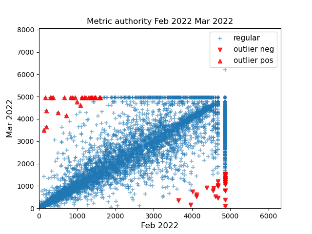
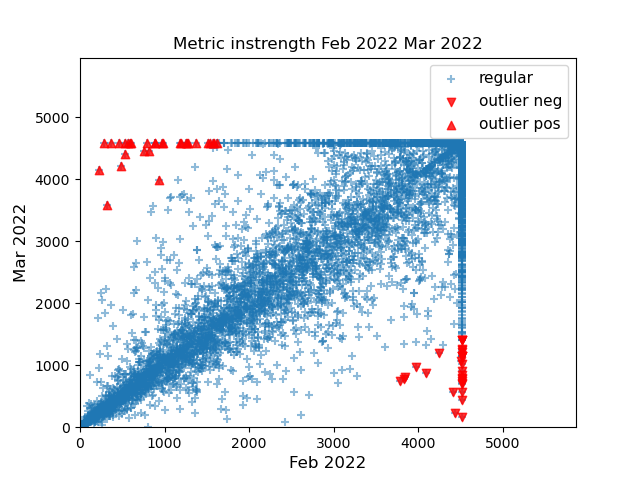
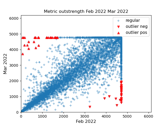
(a)

Figure 4: Step 5 of the pipeline applied on the dataset. The data points in red are the top 30 nodes by residual that are gaining (_pos) and losing (_neg) positions in the rankings from Feb 2022 to Mar 2022.

Optionally, step 6 can be applied to filter out nodes that are considered has irrelevant for the specific context of application. This was done under the guidance of the AFC experts, that were provided with a final list of potential anomalies that did not include nodes under certain thresholds of strength that depended on their own financial risk, as evaluated by the financial partner institution.

Finally, in step 7, the stratified list is created, in order to produce a single final list that collects all the relevant information from each individual centrality ranking. For this specific use case, and according to the needs of the AFC analysts involved in the experiment, each group is internally sorted according to the node’s change in volume of money exchanged with countries with high financial risk with respect to the previous timeframe (delta amount high risk).

3.3 Annotation process and evaluation of the results

The output of the steps described above was handed to the AFC analysts to undergo a process of manual validation of the results. The goals of this process are:

• to identify the presence of real anomalies (true positives) in the output list of outliers;

• to assess the goodness of the ranking methodology by evaluating if the true positives occupy the highest positions of the final sorted list.

Label	Meaning	Considered as
Relevant	Node annotated as an anomaly by AFC analysts	True Positive
Not Relevant	Node not considered as an anomaly by AFC analysts	False Positive

Table 2: Nomenclature used for the annotation task.

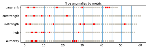
Figure 5: Position of true positives in the rankings based on the different centrality metrics.

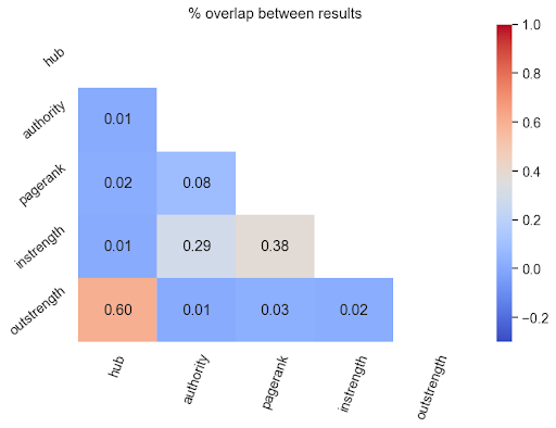
(a)

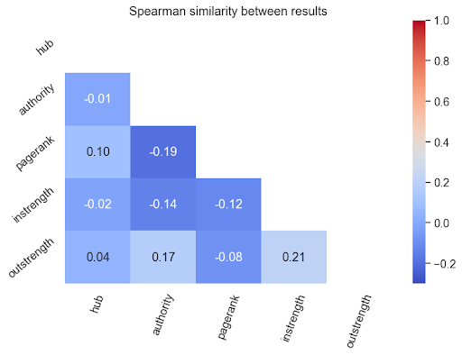
(b)

Figure 6: Correlation between the outputs on the different metrics.

The final, stratified ranking - following the removal of filtered nodes - contained 116 unique nodes, of which 14 were marked as true positives by AFC experts. In Fig. 5 we can see the ranking position of true positives according to each individual metric: considering that nodes can appear in the outputs of more than one metric, repetitions are allowed. The redundancy is measured in Fig. 6: we see, as expected given the definitions of the metrics, a good correlation between outstrength and hub score, as well as a lower but still positive correlation between instrength and both pagerank and authority scores. The Spearman correlation between these rankings is very low, suggesting that it is still worth keeping into consideration all the outputs.

In Fig. 7 we can evaluate the goodness of the final ranking by means of the precision-at-k and average p@k as described in Sec. 2.5. Here we can notice how our goal of maximising the number of true positives towards the first positions of the final outliers ranking is satisfied by the chosen ranking strategy. The precision-at-k is higher towards the first positions of the ranking and, as expected, it progressively decreases as K increases. The average precision-at-10 is 0.61, suggesting a good performance in the very first (10) ranking positions.

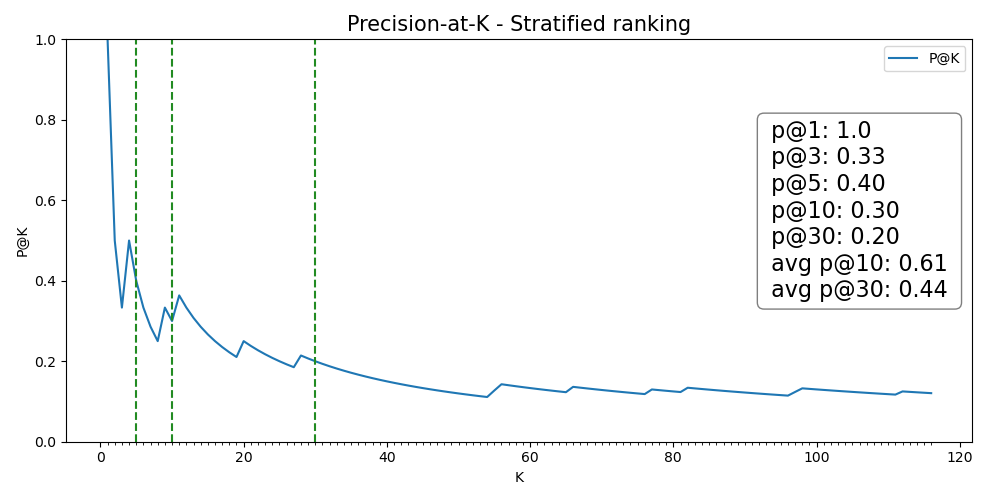
Figure 7: Precision-at-k for the stratified rankings

3.3.1 Comparison with other anomaly detection methods

The strategy of stratifying the truncated rankings based on the centrality metrics can be compared to other methods of anomaly detection based on machine learning techniques. As an example, we apply two popular techniques, OneClassSVM and IsolationForest, as discussed in Sec. 2.4 and in Fig. 2. We will not apply Elliptic Envelope, since it assumes a Gaussian distribution of the data which is not verified in our experiment.

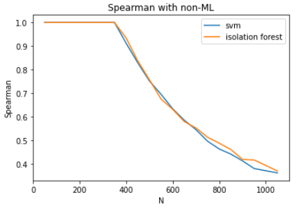
Figure 8: Comparison between the stratified ranking method and other ML-based anomaly detection techniques.

It is important to remember that the outputs of SVM and Isolation Forest, as we are considering them, are not ranked. Therefore we do not compare them with our output in terms of precision-at-k.As we can see from Fig. 8, the outputs have perfect overlap up to $N\simeq 380$, decreasing their correlation after that threshold as N increases.

3.4 Discussion

We defined and applied an anomaly detection pipeline that leverages the observation of the evolution of node rankings over time to identify potential anomalies in the system. The experimental pipeline, detailed in Sec.2.5, finds its cornerstone in the examination of temporal stability across the various centrality metrics: the observed consistency in node rankings, quantified through Spearman correlation and Normalized Similarity measures against baseline rankings (as depicted in Fig. 3), serves to identify the needed condition of stability that is then used to identify the outliers. Combining the list of outliers according to each centrality measure in a single, ranked list of potential anomalies enables us to finally meet the requirements outlined in Sec. 1.2. Indeed, considering the above mentioned requirements, the methodology defined and tested in this experiments produced the following outputs:

• O1: the final output of the algorithm is a sorted list that maximises the probability of finding true positives at the top positions of the final output. This answers assumption A1: the process of verifying anomalies is time-consuming, and the ideal expert system would provide the analyst with a possibly small set of nodes that are very likely to be actual anomalies;

• O2: as assumption A2 states, even the expert cannot confirm whether the node identified as an actual anomaly corresponds to an actual violation, until the appropriate information is examined by the competent authority. In order to reduce the chance of false positives, exogenous information was introduced as a further filtering step, incorporating the knowledge of the domain expert in the system;

• O3: finally, as outlined in assumption A3, a full explainability of the reported anomalies is required by regulators. While leveraging the embedded complexity of the financial network, our approach ensures transparency and clarity in the interpretation of results thanks to the clear interpretation of centrality metrics. This aligns with the need for regulatory actions to have clear rationales behind them.

This methodology was tested on a specific time window - the months of February and March 2022 - and the validation of the output by AFC experts constitutes a positive feedback. Of the 116 unique nodes handed to the experts following all the steps of the pipeline, 14 are confirmed as true positives worth of further investigations by the analysts and the competent authorities. The final output performs well with respect to the requirement R1 defined in Sec. 1.2, with good levels of precision-at-k for the top positions of the rankings and an average precision-at-10 of 0.61. A comparison of our output with the application of other methods of anomaly detection based on unsupervised learning algorithms, such as OneClassSVM and Isolation Forest, shows a perfect overlap regardless of the length N of the output for high values on N, that go well beyond our region of interest.

4 Conclusions

In this work, we proposed a novel methodology to detect outliers in financial graphs. It leverages the insights provided by network analysis and centrality measures to produce a ranked output of potential anomalies, following a ranking scheme that is typical of ranked information retrieval. This approach was designed based on the assumptions and the requirements explained in Sec. 1.2: it entirely revolves around simplifying the life of the AFC expert, who will need to minimise the time spent navigating through the large amount of complex data while looking for potential anomalies in transactions data.

This methodology aims at filtering out the majority of data points that follow what is identified as a normal behaviour, leaving only a reduced number of items to the attention of the expert. Given the specific context of application, there are no expectations whatsoever about the number of anomalies, nor knowledge about specific behaviour that should be looked for. For this reason, a good choice of network metrics - combined with a precise ranking strategy and, whenever possible, with quantitative domain knowledge, is crucial in ensuring that, even if an arbitrary small choice is made in terms of output size, the probability of finding real anomalies is maximised. Furthermore, every node identified as a potential anomaly has been included in the final output due to its unexpected behaviour with respect to one or more node centrality metrics, ensuring a full explainability of the result. To the best of our knowledge, no similar approach has yet been tested in AFC practices. It constitutes a radical shift from the current AFC methodologies, providing the AFC analysts with a top-down view of the system, enabling them to uncover potential threats that could have gone unnoticed otherwise, or could have required a substantially higher effort.

While this method has been developed and tested within the financial domain, it can be easily applied to other context. Potentially, every system that can be modeled through graphs and that evolves in time can be studied with this approach. Potential extensions of this methodology could involve applying it and, eventually, tailoring it to other domains, such us biology and genomics, or social networks. While we leave this as future work, we believe that these results constitute a positive contribution in improving the state of the art on network analysis applied to the detection of anomalies in the financial domain, helping AFC analysts in a delicate context where, due to an intricate tangle of contextual and regulatory reasons, the firepower of DL-based methods sometimes cannot be deployed.

References

- [1] S. Brin and L. Page. The anatomy of a large-scale hypertextual web search engine. Computer networks and ISDN systems, 30(1-7):107–117, 1998.
- [2] V. Chandola, A. Banerjee, and V. Kumar. Anomaly detection: A survey. ACM Comput. Surv., 41(3), jul 2009. doi: 10 . 1145/1541880 . 1541882
- [3] C.-C. Chang and C.-J. Lin. Libsvm: a library for support vector machines. ACM transactions on intelligent systems and technology (TIST), 2(3):1–27, 2011.
- [4] Z. Chen, D. V.-K. Le, E. Teoh, A. Nazir, E. Karuppiah, and K. Lam. Machine learning techniques for anti-money laundering (aml) solutions in suspicious transaction detection: a review. Knowledge and Information Systems, 57, 11 2018. doi: 10 . 1007/s10115-017-1144-z
- [5] C. Cortes and V. Vapnik. Support-vector networks. Machine learning, 20:273–297, 1995.
- [6] B. Dumitrescu, A. Băltoiu, and Ş. Budulan. Anomaly detection in graphs of bank transactions for anti money laundering applications. IEEE Access, 10:47699–47714, 2022.
- [7] A. Fronzetti Colladon and E. Remondi. Using social network analysis to prevent money laundering. Expert Systems with Applications, 67:49–58, 2017. doi: 10 . 1016/j . eswa . 2016 . 09 . 029
- [8] O. Garcia-Bedoya, O. Granados, and J. Burgos. Ai against money laundering networks: the colombian case. Journal of Money Laundering Control, ahead-of-print, 06 2020. doi: 10 . 1108/JMLC-04-2020-0033
- [9] I. G. García and A. Mateos. Use of Social Network Analysis for Tax Control in Spain. Hacienda Pública Española / Review of Public Economics, 239(4):159–197, November 2021.
- [10] V. Hodge and J. Austin. A survey of outlier detection methodologies. Artificial Intelligence Review, 22:85–126, 10 2004. doi: 10 . 1023/B:AIRE . 0000045502 . 10941 . a9
- [11] J. Jiang, Y. Hu, X. Li, W. Ouyang, Z. Wang, F. Fu, and B. Cui. Analyzing online transaction networks with network motifs. In Proceedings of the 28th ACM SIGKDD Conference on Knowledge Discovery and Data Mining, pp. 3098–3106, 2022.
- [12] R. Kaur and S. Singh. A survey of data mining and social network analysis based anomaly detection techniques. Egyptian Informatics Journal, 17(2):199–216, 2016. doi: 10 . 1016/j . eij . 2015 . 11 . 004
- [13] J. M. Kleinberg. Hubs, authorities, and communities. ACM computing surveys (CSUR), 31(4es):5, 1999.
- [14] D. V. Kute, B. Pradhan, N. Shukla, and A. Alamri. Deep learning and explainable artificial intelligence techniques applied for detecting money laundering–a critical review. IEEE Access, 9:82300–82317, 2021. doi: 10 . 1109/ACCESS . 2021 . 3086230
- [15] Z. Liu, D. Zhou, Y. Zhu, J. Gu, and J. He. Towards fine-grained temporal network representation via time-reinforced random walk. Proceedings of the AAAI Conference on Artificial Intelligence, 34(04):4973–4980, Apr. 2020. doi: 10 . 1609/aaai . v34i04 . 5936
- [16] J. Pan. Deep set classifier for financial forensics: An application to detect money laundering, 2022. doi: 10 . 48550/ARXIV . 2207 . 07863
- [17] D. Savage, X. Zhang, X. Yu, P. Chou, and Q. Wang. Anomaly detection in online social networks. Social Networks, 39:62–70, 2014. doi: 10 . 1016/j . socnet . 2014 . 05 . 002
- [18] A. Urbinati, E. Galimberti, and G. Ruffo. Measuring scientific brain drain with hubs and authorities: A dual perspective. Online Social Networks and Media, 26:100176, 2021.
- [19] V. Van Vlasselaer, L. Akoglu, T. Eliassi-Rad, M. Snoeck, and B. Baesens. Guilt-by-constellation: Fraud detection by suspicious clique memberships. In 2015 48th Hawaii International Conference on System Sciences, pp. 918–927. IEEE, 2015.
- [20] V. Van Vlasselaer, C. Bravo, O. Caelen, T. Eliassi-Rad, L. Akoglu, M. Snoeck, and B. Baesens. Apate: A novel approach for automated credit card transaction fraud detection using network-based extensions. Decision Support Systems, 75:38–48, 2015.
- [21] V. Van Vlasselaer, T. Eliassi-Rad, L. Akoglu, M. Snoeck, and B. Baesens. Afraid: fraud detection via active inference in time-evolving social networks. In Proceedings of the 2015 IEEE/ACM International Conference on Advances in Social Networks Analysis and Mining 2015, pp. 659–666, 2015.
- [22] V. Van Vlasselaer, T. Eliassi-Rad, L. Akoglu, M. Snoeck, and B. Baesens. Gotcha! network-based fraud detection for social security fraud. Management Science, 63(9):3090–3110, 2017.