READS-V: Real-time Automated Detection of Epileptic Seizures from Surveillance Videos via Skeleton-based Spatiotemporal ViG

Abstract

An accurate and efficient epileptic seizure onset detection system can significantly benefit patients. Traditional diagnostic methods, primarily relying on electroencephalograms (EEGs), often result in cumbersome and non-portable solutions, making continuous patient monitoring challenging. The video-based seizure detection system is expected to free patients from the constraints of scalp or implanted EEG devices and enable remote monitoring in residential settings. Previous video-based methods neither enable all-day monitoring nor provide short detection latency due to insufficient resources and ineffective patient action recognition techniques. Additionally, skeleton-based action recognition approaches remain limitations in identifying subtle seizure-related actions. To address these challenges, we propose a novel skeleton-based spatiotemporal vision graph neural network (STViG) for efficient, accurate, and timely REal-time Automated Detection of epileptic Seizures from surveillance Videos (READS-V). Our experimental results indicate STViG outperforms previous state-of-the-art action recognition models on our collected patients’ video data with higher accuracy (5.9% error) and lower FLOPs (0.4G). Furthermore, by integrating a decision-making rule that combines output probabilities and an accumulative function, our READS-V system achieves a 5.1 s EEG onset detection latency, a 13.1 s advance in clinical onset detection, and zero false detection rate. The code is available at: https://github.com/xuyankun/STViG-for-READS-V

1 Introduction

As a common neurodegenerative disorder, epilepsy affects approximately $1\%$ population worldwide [27, 35]. A reliable epileptic seizure onset detection system can benefit patients significantly, because such a system equipped with accurate algorithms can promptly alert a seizure onset. According to previous studies [34, 32, 17], they predominantly focused on designing seizure detection algorithms based on electroencephalograms (EEGs). Although EEG can sense subtle brain changes just after a seizure begins, the use of scalp or implantable EEG devices often causes discomfort to patients and restricts them to hospital epilepsy monitoring units (EMUs). Consequently, there is a growing interest in developing an accurate video-based seizure detection system that could alleviate the discomfort associated with EEG helmets and facilitate remote monitoring of epileptic patients in residential settings [41]. However, the development of video-based seizure detection is hindered by several challenges as follows:

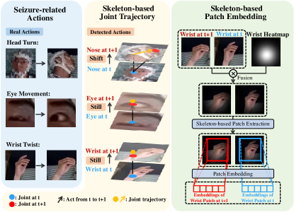
Figure 1: Motivation of skeleton-based patch embedding for seizure-related action recognition. The left shows real seizure-related actions; The middle shows challenges of traditional skeleton-based approaches; The right shows our strategy to address challenges.

(1) Lack of datasets. Seizure-related video data collection is substantially time-consuming and requires doctoral expertise to annotate the different seizure-related periods. And, surveillance video recordings from the hospital EMUs contain highly sensitive information, they often capture the faces of patients, their families, and healthcare staff. This sensitivity raises privacy concerns and complicates the data collection process. Based on these reasons, there is no public video data intended for seizure study yet, which hinders the development of video-based seizure detection research.

(2) Lack of effective analytic tools. Fundamentally, video-based seizure detection is an action recognition task, requiring the analysis of complex seizure-related actions in epileptic patients. Prior research indicates that existing methods struggle with achieving short detection latency and are often limited to nocturnal seizures when using raw RGB frames [46, 42]. While skeleton-based approaches powered by graph convolutional networks (GCNs) offer several advantages over RGB-based methods [9, 47, 21], there also encounter significant limitations in the context of seizure detection. Firstly, pre-trained pose estimation models [4, 10, 2, 26, 37] cannot be applied to epileptic patients’ action recognition directly due to the complexity of epileptic patient scenarios. These models suffer from unusual clothing, varied camera angles, and intricate behaviors of patients, leading to difficulties in accurately tracking patient skeletons. Secondly, as shown in Fig. 1, there are inherent difficulties in recognizing certain seizure-related actions using traditional skeleton-based approaches. For example, When a patient turns head, the tracking of the nose joint across frames can create ambiguity, making it unclear whether the patient is turning head or simply shifting it. Similarly, eye movements or wrist/ankle twists can only be tracked as static points instead of any changes. Furthermore, finger/toe movement also cannot be tracked by the model with the mainstream 17-keypoint template [24, 1].

(3) Detection latency and false detection rate. Detection latency is a critical metric in a seizure detection system, representing the time gap between the real onset of a seizure and the detected onset. A shorter detection latency is highly desirable since it enables the system to alert caregivers before the onset of severe tonic-clonic symptoms, allowing timely interventions to prevent secondary injuries from a seizure attack. Also, false detection rate (FDR) is important in determining the quality of a seizure detection system [40, 36]. In terms of EEG time-series, the characteristics of EEG signals during the ictal period significantly differ from those in a healthy status, particularly in the frequency characteristics. In video-based detection, however, many normal patient behaviors closely resemble seizure-related actions. This similarity presents a challenge in accurately distinguishing between them, especially when decisions are based on a single video clip.

In this study, we propose a novel skeleton-based spatiotemporal vision graph neural network (STViG), designed for efficient, accurate, and timely REal-time Automated Detection system of epileptic Seizures from surveillance Videos (READS-V). We address the aforementioned limitations by offering the following contributions: (1) We acquire a dataset of epileptic patient data from hospital EMUs and train a custom patient pose estimation model by manual pose annotations; (2) As expressed in the Fig. 1, instead of using skeleton-based coordinates, our STViG model utilizes skeleton-based patch embeddings as inputs to address remaining challenges. We also introduce a partitioning strategy in STViG to learn spatiotemporal inter-partition and intra-partition representations; (3) We generate the probabilities instead of binary classifications as outputs in this application, and make use of accumulative probability strategy to obtain shorter detection latency and lower FDR in real-time scenarios.

2 Related Work

Video-based seizure detection. There have been several efforts paid to video-based seizure detection or jerk detection since 2012 [6, 42, 19, 13], but they neither utilized DL approaches to achieve accurate performance nor supervised patients 24/7 by video monitoring. Since 2021, two recent works [46, 20] made use of DL models to improve the video-based seizure detection performance, however, one cannot provide all-day video monitoring with short latency and another one did not utilize a common RGB camera for video monitoring. Our proposed STViG framework can provide accurate and timely 24/7 video monitoring.

Action recognition. There are two mainstream strategies for action recognition tasks, one is 3D-CNN for RGB-based action recognition, and the other one is skeleton-based action recognition. Many 3D-CNN architectures [12, 11, 18, 38, 39] have been proven to be effective tools for learning spatiotemporal representations of RGB-based video streams, they are widely applied to video understanding and action recognition tasks. Compared to RGB-based approaches with a large number of trainable parameters, skeleton-based approaches perform better in both accuracy and efficiency because they only focus on the skeleton information which is more relevant to the actions, and can alleviate contextual nuisances from raw RGB frames. Several GCN-based approaches [30, 23, 33, 5, 45] were proposed to achieve great performance in skeleton-based action recognition. [9] proposed PoseConv3D to combine 3D-CNN architecture and skeleton-based heatmaps, and proposed its variant RGBPoseConv3D to fuse RGB frames to obtain better performance. However, all aforementioned action recognition models show weaknesses in analyzing seizure-related actions, which include subtle behavioral changes when seizures begin. In this work, we propose STViG model to address this challenge.

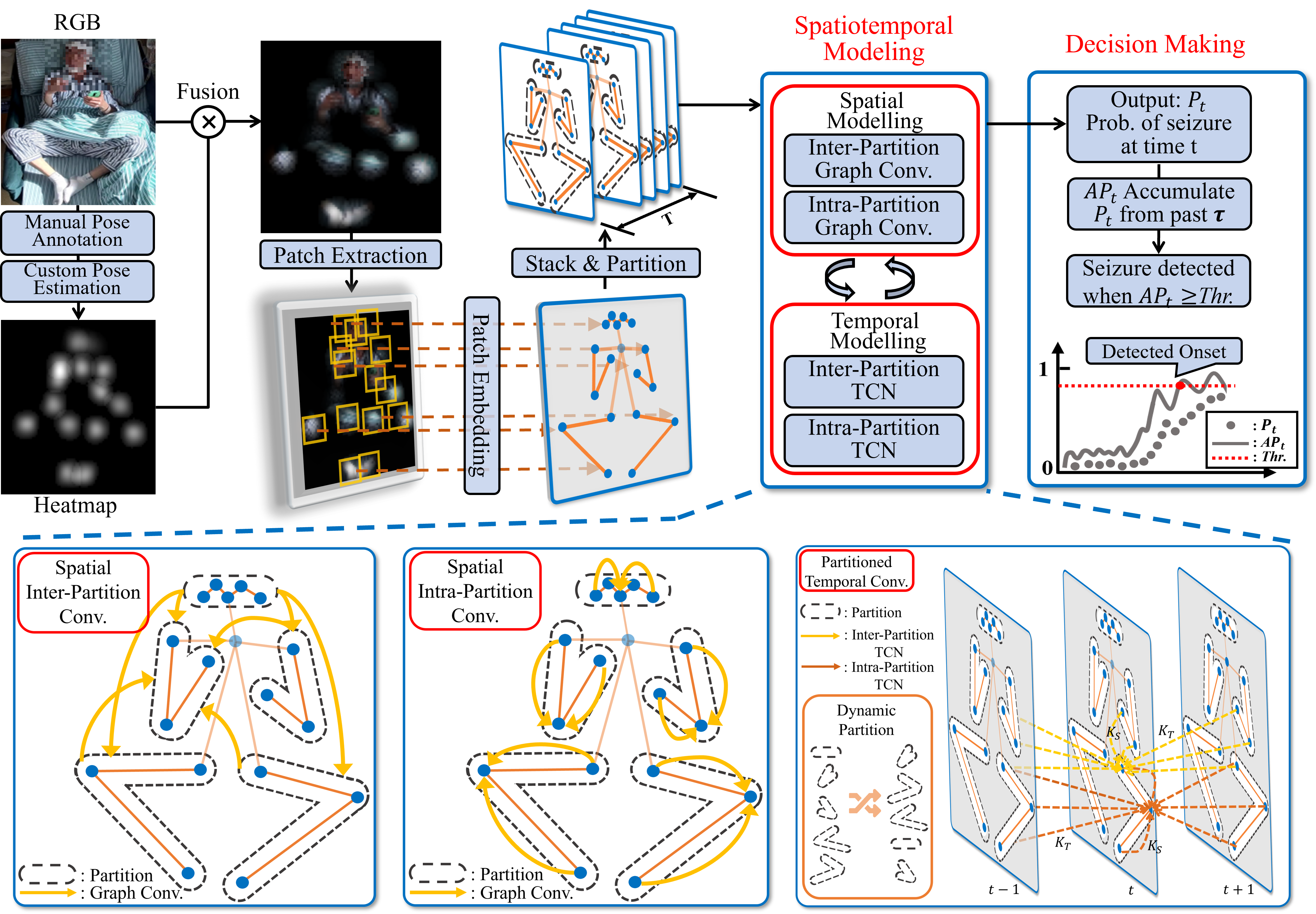
Figure 2: Proposed skeleton-based STViG framework for READS-V system. Starting from raw RGB frames, we extract skeleton-based patches around each joint by fusing RGB frame and pose heatmap. These patches are then transformed into feature vectors through a patch embedding layer. We utilize a partitioning strategy to divide skeleton-based embeddings into several partitions. The STViG model, comprising both spatial and temporal modeling modules, is designed to learn inter- and intra-partition representations, thereby facilitating a better understanding of seizure-related actions. The bottom three figures express how the partitioning strategy works. After generating probability outputs, an accumulative probability strategy is used to enhance the performance of seizure onset decisions.

Vision graph neural network. [14] first proposed vision graph neural networks (ViG) as an efficient and effective alternative backbone for image recognition. Since then many ViG variants [15, 28, 49, 43] have been proposed to handle various applications. Inspired by ViG, we first propose STViG to extend ViG to accomplish a skeleton-based action recognition task from videos.

3 READS-V Framework

Fig. 2 presents an overview of skeleton-based STViG framework designed for READS-V. The process Starting begins with a video clip composed of consecutive RGB frames, we train the custom pose estimation model to generate joint heatmaps, then fuse these heatmaps and raw frames to construct skeleton-based patches. Prior to being processed by the STViG model, these patches are transformed into feature vectors through a trainable patch embedding layer. Additionally, the joints are grouped into several partitions, enhancing our model’s ability to recognize seizure-related actions. During the STViG processing phase, we conduct spatial and temporal modeling respectively, and utilize partition structure to learn inter-partition and intra-partition representations. STViG model outputs probabilities instead of binary classes for video clips, then a decision-making rule integrating probabilities and accumulative function can achieve shorter detection latency and lower FDR. The subsequent subsections will provide detailed explanations of each step in this process.

3.1 Custom pose estimation

The STViG framework relies on a pose estimation algorithm to extract joint heatmaps at first. However, when we tested several mainstream pre-trained pose estimation models on our patient video data, the results were unsatisfactory. These models failed to accurately track the locations of patients and their joints. Therefore, we have to train our custom pose estimation model.

We manually annotated 580 frames containing various behaviors during the both ictal periods and healthy status across all patients, then utilized lightweight-openpose [29] model as basis for our training for its efficient deployment. Eventually, we achieved a custom pose estimation model for all patients.

3.2 Patch extraction and patch embedding

In custom pose estimation algorithm, each joint is associated with a heatmap generated by a 2D Gaussian map [3]. We make use of this heatmap as filters to fuse the raw RGB frames, then extract a small patch around each joint from the fused image. However, determining the optimal size of the Gaussian maps to capture the regions of interest is a challenge during the training phase of the pose estimation model. To address this, we manually extract the patch $\mathbf{p}_{it}$ of $i$-th ($i=1,2...,N$) joint at frame $t$ by generating a Gaussian map with adjustable $\sigma$ for each joint to filter the raw RGB frame $\textbf{{I}}_{t}$:

$$\mathbf{p}_{it}=exp(-\frac{(m-x_{it})^{2}+(n-y_{it})^{2}}{2\sigma^{2}})\otimes\textbf{{I}}_{t}(m,n)$$ (1)

where $|m-x_{i}|\leq H/2$, $|n-y_{i}|\leq W/2$. $(H,W)$, $(m,n)$ and $(x_{it},y_{it})$ respectively stand for the size of patches, the coordinate of image pixels, and the location of $i$-th joint at frame $t$. The $\sigma$ controls the shape of 2D Gaussian kernels. As a result, we are able to extract a sequence of skeleton-based patches $\mathbf{P}\in\mathbb{R}^{N\times T\times H\times W\times 3}$ from each video clip, then a patch embedding layer transforms patches into 1D feature vectors $\mathbf{X}\in\mathbb{R}^{N\times T\times C}$.

3.3 Graph construction with partition strategy

Given a sequence of skeleton-based patch embeddings, we construct an undirected skeleton-based spatiotemporal vision graph as $\mathcal{G}=(\mathcal{V},\mathcal{E})$ on this skeleton sequence across $N$ joints and $T$ stacked frames. Each node in the node set $\mathcal{V}=\left\{v_{it}|i=1,2,...,N,t=1,2...,T\right\}$ is associated with feature vectors $\mathbf{x}_{it}\in\mathbb{R}^{C}$.

In this study, we proposed a partitioning strategy to construct graph edges between nodes. According to Openpose joint template, which contains 18 joints, we focus on 15 joints by excluding three (l_ear, r_ear, neck) as redundant. These 15 joints are divided into 5 partitions, each comprising three joints (head: nose, left/right eye; right arm: right wrist/elbow/shoulder; right leg: right hip/knee/ankle; left arm: left wrist/elbow/shoulder; left leg: left hip/knee/ankle). In our STViG, we conduct both spatial and temporal modeling for the graph. Spatial modeling involves constructing two subsets of edges based on different partition strategies: inter-partition edge set, denoted as $\mathcal{E}_{inter}=\left\{v_{it}v_{jt}|i\in\mathbf{Part}_{p1},j\in\mathbf{Part}_{p2},p1\neq p2\right\}$ and intra-partition edge set, denoted as $\mathcal{E}_{intra}=\left\{v_{it}v_{jt}|(i,j)\in\mathbf{Part}_{p}\right\}$, where $p,p1,p2=1,...,5$. As shown in the bottom left two schematic figures in Fig. 2, each node is connected to the nodes from all other partitions in the inter-partition step, and each node is only connected to the other nodes within the same partition in the intra-partition step. The bottom-left two figures of Fig. 2 visualize the graph construction with partitioning strategy.

For temporal modeling, we consider neighbors of each node within a $K_{S}\times K_{T}$ in both temporal and spatial dimensions. The temporal edge set is denoted as $\mathcal{E}_{T}=\left\{v_{it}v_{j(t+1)}|d(v_{it},v_{jt})\leq K_{S}/2,d(v_{it},v_{i(t+1)})\leq K_{T}/2\right\}$, where $d$ is the distance between two nodes. To facilitate the partitioning strategy, we arrange the joints with their partitions in a 1D sequence. Thus, if $K_{S}=3$, as shown in the bottom-right figure of Fig. 2, the middle joint of a partition aggregates only from intra-partition nodes over $K_{T}$ frames, while the border joint of a partition aggregates from inter-partition nodes over $K_{T}$ frames.

3.4 Partitioning spatiotemporal graph modeling

Spatial Modeling. The proposed skeleton-based STViG aims to process the input features $\mathbf{X}\in\mathbb{R}^{N\times T\times C}$ into the probabilities of seizure onset. Starting from input feature vectors, we first conduct spatial modeling to learn the spatial representations between nodes at each frame by inter-partition and intra-partition graph convolution operation as $\mathcal{G}^{{}^{\prime}}=F_{intra}(F_{inter}(\mathcal{G},\mathcal{W}_{inter}),\mathcal{W}_{intra})$, where $F$ is graph convolution operation, specifically we adopt max-relative graph convolution [22, 14] to aggregate and update the nodes with fully-connected (FC) layer and activation function:

$$\mathbf{x}^{{}^{\prime}}_{it}=\sigma(Linear([\mathbf{x}_{it},max({\mathbf{x}_{jt}-\mathbf{x}_{it}}|j\in\mathcal{N}^{t}(\mathbf{x}_{it}))]))$$ (2)

where $\mathcal{N}^{t}(\mathbf{x}_{it})$ is neighbor nodes of $\mathbf{x}_{it}$ at frame $t$, $Linear$ is a FC layer with learnable weights and $\sigma$ is activation function, e.g. ReLU. The only difference between $F_{inter}$ and $F_{intra}$ depends on $\mathcal{N}^{t}(\mathbf{x}_{it})$ is from $\mathcal{E}_{inter}$ or $\mathcal{E}_{intra}$. Given input feature vectors at frame $t$, denoted as $\mathbf{X}_{t}\in\mathbb{R}^{N\times C}$, the graph convolution processing as Eq. 2 can be denoted as $\mathbf{X}^{{}^{\prime}}_{t}=MRGC(\mathbf{X}_{t})$, then the partitioning spatial graph processing module in STViG would be:

$$\mathbf{X}_{t}^{{}^{\prime\prime}} =\sigma(MRGC(\mathbf{X}_{t}W_{in\_inter})W_{out\_inter}+X_{t})$$ (3)

$$\mathbf{X}_{t}^{{}^{\prime}} =\sigma(MRGC(\mathbf{X}_{t}^{{}^{\prime\prime}}W_{in\_intra})W_{out\_intra}+X_{t})$$

We add original input $\mathbf{X}_{t}$ as a residual component to both two partitioning spatial modeling, which is intended to avoid smoothing and keep diversity of features during the model training [16, 7]. We keep output dimension of every learnable layer is same as input dimension, so that we achieve output feature $\mathbf{X}^{{}^{\prime}}\in\mathbb{R}^{N\times T\times C}$ when we stack $T$ frames $\mathbf{X}^{{}^{\prime}}_{t}\in\mathbb{R}^{N\times C}$ after spatial modeling.

Temporal Modeling. Given the dimension of output features after spatial modeling is $N\times T\times C$, and we order the partitions (containing joints) in a 1D sequence, so that we can naturally consider the input for the temporal modeling as a 3D volume, denoted as $\mathbf{X}\in\mathbb{R}^{1\times N\times T\times C}$. According to the construction of graph in temporal modeling $\mathcal{G}=(\mathcal{V},\mathcal{E}_{T})$, we can adopt convolution operation to aggregate and update nodes:

$$\mathbf{x}^{{}^{\prime}}_{i}=\sum_{j}^{1}\sum_{j}^{K_{S}}\sum_{j}^{K_{T}}w_{ij}\mathbf{x}_{i}$$ (4)

Inspired by [9, 45, 16], we utilize residual 3D-CNN architecture, denoted as $Conv$, to conduct temporal graph modeling as Eq. 4 for its simplicity:

$$\mathbf{X}^{{}^{\prime}}=Conv{(1)}(Conv{(1,K_{S},K_{T})}(Conv{(1)}(\mathbf{X})))+\mathbf{X}$$ (5)

where $(1)$ and $(1,K_{S},K_{T})$ are kernel size for the 3D convolution operation.

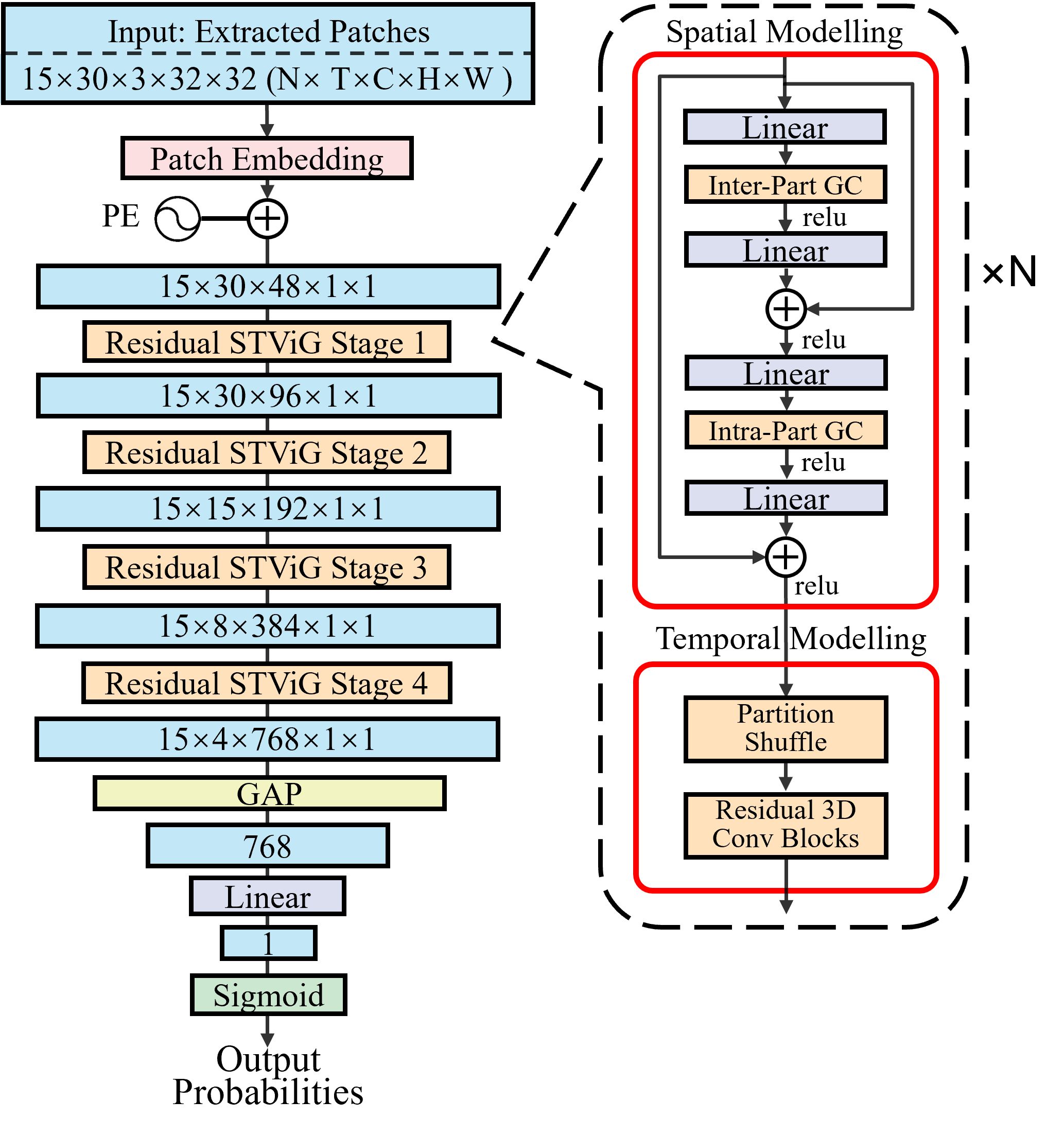
Figure 3: STViG architecture. Begin with patches extracted from the target video clip, input and positional embedding layers transform patches into feature vectors. STViG consists of four residual stages with expansion and downsampling operations. Each stage contains several proposed spatiotemporal learning layers. The output probability with dimension 1 is generated from a Sigmoid function. $N,T,C$ denotes the number of joints, frames and channels, and $H,W$ stand for the height and width of extracted patches.

Layer name	Output size T	STViG-Light/Base
(Patches)	30	$(1\times 15\times T\times 32\times 32\times 3)$
Stem	30	$32\times 32,12/24$
(Features)	30	$(1\times 15\times T\times C)$
Stage1	30	$\begin{bmatrix}E=12,12/24\\ E=2,12/24\\ 1\times 1^{2},12/24\\ 1\times 3^{2},12/24\\ 1\times 1^{2},24/48\end{bmatrix}\times 2$
Stage2	15	$\begin{bmatrix}\ E=12,24/48\\ \ E=2,24/48\\ \ 1\times 1^{2},24/48\\ \ 1\times 3^{2},24/48\\ \ 1\times 1^{2},48/96\end{bmatrix}\times 2$
Stage3	8	$\begin{bmatrix}\ E=12,48/96\\ \ E=2,48/96\\ \ 1\times 1^{2},48/96\\ \ 1\times 3^{2},48/96\\ \ 1\times 1^{2},96/192\end{bmatrix}\times 6$
Stage4	4	$\begin{bmatrix}\ E=12,96/192\\ \ E=2,96/192\\ \ 1\times 1^{2},96/192\\ \ 1\times 3^{2},96/192\\ \ 1\times 1^{2},192/384\end{bmatrix}\times 2$
Head	1	GAP, 1-d FC, Sigmoid
FLOPS		0.44G/1.76G

Table 1: Details of two versions of STViG. In Stem layer, $32\times 32,C$ is kernel size and output channels of Conv2D implemented on input patches ($H\times W$). Then we utilize 4-stage spatiotemporal modeling to process features. $E,C$ denotes the number of constructed edges between neighbors and output channels for spatial modeling, $1\times K_{S}\times K_{T},C$ denotes kernel size and output channels of 3D-CNN in temporal modeling. In practice, we render 3 for both $K_{S}$ and $K_{T}$.

3.5 STViG network architecture

Fig. 3 is the detailed architecture of proposed STViG network including the size of features at each layer. We keep feature size in spatial modeling, and implement downsampling at the last layer of each residual temporal block. After four residual STViG stages, we make use of global average pooling to generate a 1D feature vector, then one FC layer and sigmoid function are connected to generate output probabilities. We provide two versions of STViG models: STViG-Base and STViG-Light respectively based on different model depths and feature expansions, which are shown in Table 1.

In spatial modeling, $E=12$ and $E=2$ represent the number of edges/neighbors in inter-partition and intra-partition graph convolution, respectively. The spatial modeling phase always keeps the output channels unchanged. In temporal modeling, we set $K_{S}=3$ for simultaneously implementation of inter-partition and intra-partition temporal convolution network (TCN) operation, and set $K_{T}=3$ for considering only one frame before and after the current frame. The residual 3D-CNN block is used to expand feature dimension and downsample temporal frames.

Positional embedding. In previous studies, either skeleton-based ST-GCNs which input coordinate triplets or RGB-/Heatmap-based methods made use of specific joint coordinates or whole body context with global positional information. In this work, however, input patches in 1D sequence do not provide any positional information. Thus, we add a positional embedding to each node feature vector. Here we propose 3 different ways to inject positional information: (1) Add learnable weight $\mathbf{x}_{it}=\mathbf{x}_{it}+\mathbf{e}_{it}$; (2) Concatenation with joint coordinates $\mathbf{x}_{it}=[\mathbf{x}_{it},(x_{it},y_{it})]$; (3) Add embeddings of joint coordinates: $\mathbf{x}_{it}=\mathbf{x}_{it}+Stem(x_{it},y_{it})$;

Dynamic partitions. Since the partitions are arranged as a 1D sequence, each partition is only connected to 1 or 2 adjacent partitions, it cannot consider all other partitions as spatial modeling does. Thus, we obtain the dynamic partitions by conducting partition shuffle before temporal graph updating. It is noted that we only shuffle the partitions, and the order of joints within a partition is unchanged.

3.6 Seizure onset decision-making

Inspired by [44], after generating output probabilities $P_{t}$ by proposed skeleton-based STViG model for video clips at time t, we can accumulate a period $\tau$ of previously detected probabilities as accumulative probabilities $AP_{t}=\sum_{i=t-\tau}^{t}P_{i}$ with detection rate $r$, then make a seizure onset decision at time $t_{onset}$ when accumulative probabilities reach a decision threshold $DT$: $t_{onset}=AP_{t}>DT$. We measure the distance between $t_{onset}$ and EEG onset as latency of EEG onset $L_{EO}$, and the distance between $t_{onset}$ and clinical onset as latency of clinical onset $L_{CO}$.

4 Experiments

4.1 Dataset

Data acquisition. We acquire surveillance video data of epileptic patients from a hospital, this dataset includes 14 epileptic patients with 33 tonic-clonic seizures. Patients in the hospital EMUs are supervised by Bosch NDP-4502-Z12 camera with 1920 $\times$ 1080 resolution 24/7. We extract successive frames as video clips for real-time processing. Each video clip spans a duration of $5s$ with the original rate of 30 FPS. To enhance the efficiency of our real-time analysis, we apply fixed stride sampling to reduce the frame count from the original 150 frames to 30 frames.

Data labeling. How to label the video clips is a challenge in video-based seizure detection. Typically, EEG-based seizure detection is treated as a binary classification task, distinguishing between interictal (pre-seizure) and ictal (during-seizure) periods. Medical experts annotate the moment from interictal to ictal periods in EEG recordings as the EEG onset. However, in video analysis, the transition from normal to seizure behavior is not as immediate. For several seconds (ranging from 1 to 30 seconds) after the EEG onset, a patient’s behavior may appear only slightly abnormal or nearly normal. We refer to this phase as the transition period. The moment when patients start exhibiting clearly abnormal actions, such as jerking, convulsion, or stiffening, is defined as clinical onset. It is straightforward to label video clips as healthy status (0) before the EEG onset and as seizure status (1) after the clinical onset. These labels (0 and 1) can be interpreted as the probability or risk of seizure onset. In terms of the transition period, it is hard to assign a precise probability to each clip. Clinically, it’s observed in the transition period that patients are more likely to appear healthy closer to the EEG onset and more likely to exhibit abnormal behaviors as the time approaches the clinical onset. To address this, we use an exponential function to assign increasing probabilities to video clips during the transition period, ranging from 0 to 1. Other options for probability-increasing functions are explored in the appendix. It is noted that the probabilities of video clips depend on the end frame of video clips lying in which period. Consequently, we define this task as a probability regression task rather than a traditional classification task.

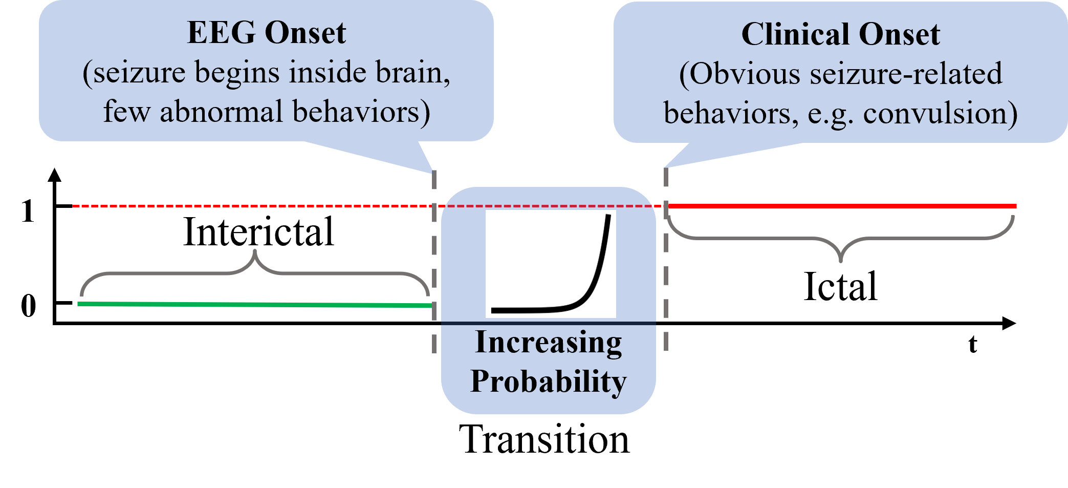
Figure 4: Data labeling of video-based seizure detection task. For each seizure, a video recording is categorized into 3 different periods: interictal (label:0), ictal (label:1), and transition (label:0 to 1 in exponential function according to clinical phenomenon).

# pat	# seizures	Interictal period	Transition period	Ictal period
14	33	2.78h	0.16h	0.35h

Table 2: Summary of dataset used in this work.

Method	Input	Backbone	Error	FLOPs	Param.
DGSTGCN [8]	Skeleton	GCN	16.7	0.50G	1.4M
RGBPoseConv3D [9]	RGB+Skeleton	3D-CNN	13.8	12.63G	3.2M
STGCN [45]	Skeleton	GCN	14.1	1.22G	3.1M
MSG3D [25]	Skeleton	GCN	11.3	1.82G	2.7M
AAGCN [31]	Skeleton	GCN	9.5	1.38G	3.7M
CTRGCN [5]	Skeleton	GCN	8.3	0.62G	1.4M
STViG-Light (Ours)	Patch	ViG	6.1	0.44G	1.4M
STViG-Base (Ours)	Patch	ViG	5.9	1.76G	5.4M

Table 3: Comparison with previous state-of-the-arts. We reproduce state-of-the-art approaches to make comparisons. Error is averaged RMSE (%) for each video clip.

Data splitting. For each seizure event, we categorize the video segments based on their timing relative to the EEG onset and clinical onset, which are annotated by medical experts. We define the period $<2min$ after clinical onset as the ictal period, and the period $<30min$ before EEG onset as the interictal period. Given that patients’ behaviors often remain unchanged for extended periods, we strive to include a variety of actions in the extracted clips. The transition period usually ranges from $1s\sim 20s$ after EEG onset for each seizure event. In our dataset, the average transition period is approximately $18.2s$ across 33 seizures. To address the imbalance in duration between interictal and other periods, we extract clips from interictal period without overlapping, and from both transition and ictal periods with $4s$ overlappings. For fair performance comparison, we randomly extract $20\%$ clips from both transition and ictal periods from each seizure, and an equivalent number of clips (20% transition + 20% ictal) are extracted from the interictal period for validation, the rest clips are for model training. In this study, we aim to train a generalized model applicable to all patients rather than a patient-specific model. Table 2 summarize the dataset we used in this study.

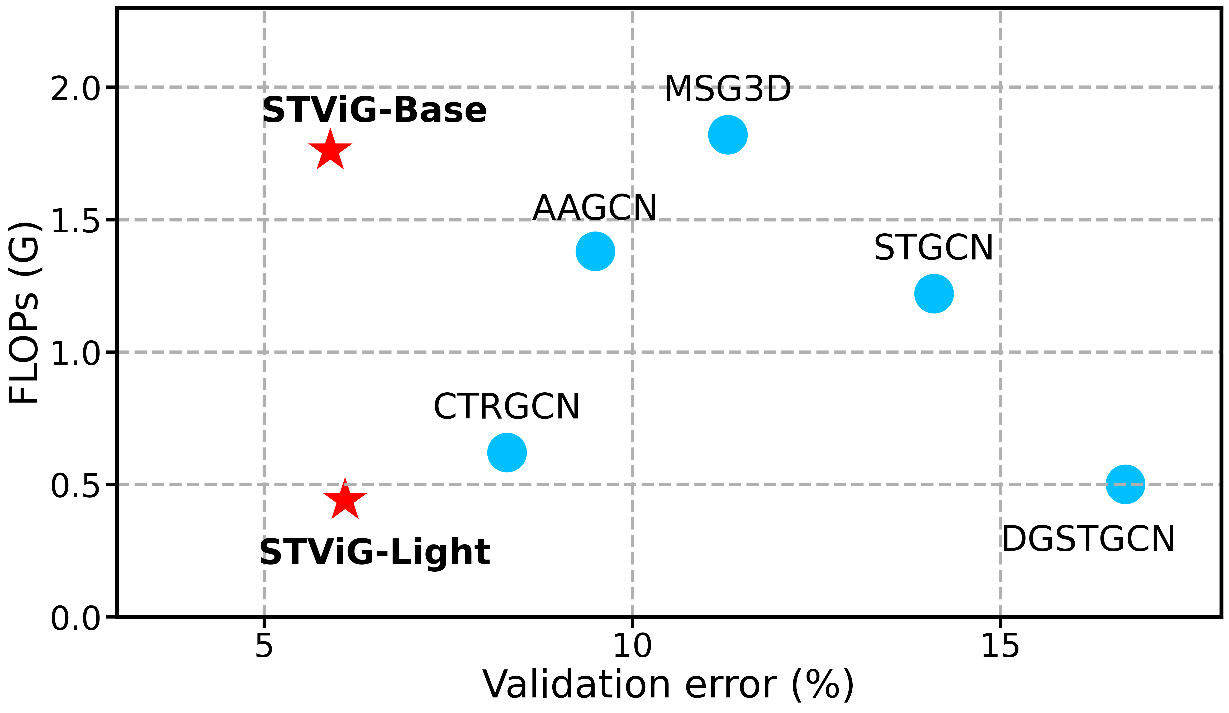
Figure 5: Comparison of performance vs. efficiency.

4.2 Experimental setting

We manually set a size of $32\times 32\ (H\times W)$ for extracted patches based on the 1920$\times$ 1080 raw frame resolution, and $\sigma$ of gaussian kernel is $0.3$. All generated outputs are connected with a Sigmoid function to map the outputs as probabilities from 0 to 1, the activation function used anywhere else is chosen as ReLU, and mean square error loss function is used to train the model. During the training phase, epoch and batch size are respectively set to $200$ and $32$, we choose Adam optimizer with 1e-4 learning rate with 0.1 gamma decay every 40 epochs and 1e-6 weight decay. We save the best model with the lowest error on the validation set.

4.3 Seizure-related action recognition performance

Our STViG-Base and STViG-Light obtain $5.9\%$ and $6.1\%$ errors across all patients. We reproduce several state-of-the-art action recognition models, conducting a grid search to optimize the learning rate and weight decay for each model. We select one CNN-based approach, RGBPoseConv3d, and 5 state-of-the-art skeleton-based approaches for the comparison. According to Table 3, two STViG models both outperform previous state-of-the-arts. We also visualize model comparison of performance vs. efficiency in Fig. 5, which highlights the advantages of STViG models. Notably, STViG-Light demonstrates strong performance in both accuracy and efficiency.

The RGBPoseConv3D model is a leading RGB-based action recognition model, it was inspired by several 3D CNN architectures [38, 11, 12] and fused RGB and skeleton as input features simultaneously. Our results reveal it performs worse than skeleton-based approaches even if it contains a large number of parameters, in our opinion, its reduced effectiveness is due to the complexities of the EMU environment, which adversely affect RGB-based methods. As for skeleton-based approaches, most perform around $10\%$ error with lower FLOPs, and CTRGCN performs the best among all skeleton-based approaches. These results underscore the superiority of our skeleton-based STViG models over both RGB-based and other skeleton-based approaches in terms of accuracy and efficiency, making them highly suitable for real-time deployment.

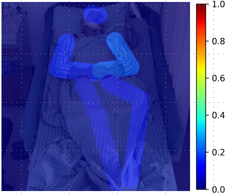
(a) Healthy status.

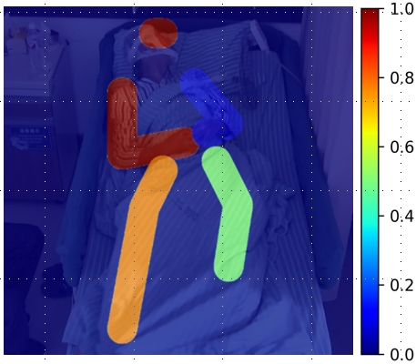
(b) Head turn (seizure begins).

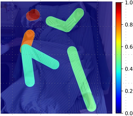
(c) Continue to act abnormally.

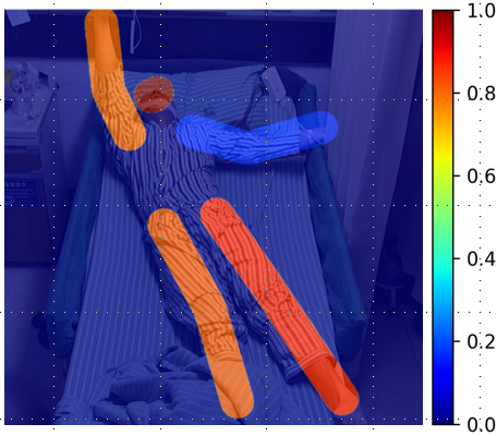
(d) Convulsion

Figure 6: Occlusion maps for model interpretability. Each image represents the end frame of the video clip. Redder partitions means more salient to the seizure-related actions.

4.4 Ablation study

We conduct ablation study with STViG-Base to evaluate the effects of positional embedding way and dynamic partition strategy on the model. In Table 4, we can see that Stem positional embedding way with dynamic partition achieves the best performance.

Effect of dynamic partition. Dynamic partition strategy shows better performance among all four types of positional embedding, which indicates that dynamic partition strategy can effectively enhance the model to learn relationships between different partitions, thereby understanding the seizure-related actions.

Effect of positional embedding. According to the results in Table 4, positional information can bring better performance for STViG model, and Stem way can outperform among three positional embedding ways. Further, we find that no positional embedding with dynamic partition can also bring a satisfactory result compared with other GCN-based approaches, which indicates that proposed STViG model has the capability to complete action recognition task without any specific or global positional information. In our point of view, the reason is that inter-partition and intra-partition representations contain enough information for action recognition no matter how these partitions are ordered or where they are.

4.5 Model interpretability

We provide interpretability with occlusion maps [48] to demonstrate the capabilities of our STViG model to learn representations of seizure-related actions between different partitions. We successively take 4 video clips of a patient from healthy status to seizure coming, as shown in Fig. 6, each image represents the end frame of corresponding clips, higher value (redder) partition means more salient to seizure-related actions, and lower value (bluer) partition means less relevant. We can see that, initially, when the patient is lying on the bed, all partitions are shown as less salient in Fig. 6(a). As the seizure begins, the patient starts to exhibit abnormal movements, such as turning the head and moving the right arm. Correspondingly, these partitions appear redder in Fig. 6(b) and Fig. 6(c), indicating their increased relevance to the seizure activity. Several seconds later, as the patient begins jerking, most partitions are shown as more salient in Fig. 6(d). This form of model interpretability provides a visual tool for doctors to efficiently analyze the progression of a seizure attack and understand the types of seizure-related actions, thereby aiding in better diagnosis and treatment planning.

Positional embedding	Dynamic Partition
	w/o   w.
None	16.9   9.1
Cat	14.8   8.9
Learn	13.4   8.6
Stem	8.4    5.9

Table 4: Ablation study. We utilize STViG-Base model to evaluate the effects of positional embedding way and dynamic partition. The shown values are averaged error (%) for each clip.

$DT$	FDR	Latency	Accumulative
			w/o	w.
0.5	0	$L_{EO}$	15.3s	10.9s
		$L_{CO}$	-2.9s	-7.3s
0.2	0	$L_{EO}$	11.4s	5.1s
		$L_{CO}$	-6.8s	-13.1s

Table 5: Seizure detection performance. We evaluate the effect of different DTs and the proposed accumulative strategy for detected latency. $DT$: decision threshold, $L_{EO}$: latency of EEG onset $L_{CO}$: latency of clinical onset, FDR: false detection rate.

4.6 Make seizure onset decision

After obtaining probabilities from consecutive video clips by STViG-Base model, we set up $\tau=3\ s,r=0.5\ s$ as mentioned in Section 3.6 to calculate $L_{EO},L_{CO}$ and FDR across all seizures. We also evaluate the effect of accumulative strategy on the detected latency, as shown in Table 5. We can see that performance without accumulative strategy is satisfactory based on accurate STViG model, but accumulative strategy with $DT=2$ can obtain much better performance where $5.1\ s\ L_{EO}$, -$13.1\ s\ L_{CO}$, which means seizure can be detected only $5.1\ s$ after seizure begins inside brain, and can alarm the seizure coming $13.1\ s$ before patients tend to exhibit serious convulsions. And a FDR of 0 is achieved by all conditions.

5 Conclusion

In this work, we propose a STViG model based on skeleton-based patch embeddings to recognize the epileptic patients’ actions effectively, experiments indicate proposed STViG model outperforms state-of-the-art action recognition approaches. It provides an accurate, efficient, and timely solution for the READS-V system to fundamentally help epileptic patients. In the future, we will collect more patient video data with various types of seizures to train a more generalized model for wider epileptic patients.

Supplementary Material

A. Visualization

First, we visualize the pose estimation performance comparison between our custom model and the public pre-trained model, as shown in Fig. 7, thereby demonstrating the limitation of public pre-trained model for tracking patient skeletons.

Second, we present the visualization of predictive probabilities of video clips obtained by STViG model from two different seizures, which is shown as . It is important to note that these frames are not successive, we are intended to show the clips with different predictive probabilities in a seizure. We can see that our model can detect subtle motion changes during the seizure beginning.

These two visualization results built in .gif format are included in the supplementary package.

B. Chosen of increasing probability function

In this study, we label the transition period from 0 to 1 in exponential function due to clinical phenomenon. We also choose two alternatives - linear and sigmoid functions to make a comparison with exponential function in STViG-Base model. We can see from Table 6 that the exponential labeling function outperforms the other two functions.

	Linear	Sigmoid	Exponential
Error	6.7%	9.4%	5.2%

Table 6: Comparisons of different increasing probability functions used for labeling transition period.

C. Detailed seizure detection performance

Table 5 has shown averaged seizure detection performance by our STViG model, and evaluates the effect of accumulative probability strategy on the detection latency performance. Here we show the detailed results for each patient including more clinical information, as shown in Table 8. We can see that our experimental subjects contain diversity in age, gender, and seizure type. The result indicates that we can detect all 33 seizures across patients (100% sensitivity) and 0 FDR, and latency can be optimized by $DT$ = 0.2 with accumulative probability strategy.

D. Comparison with state-of-the-art video-based seizure detection studies

Table 3 has already presented a performance comparison between our model and state-of-the-art action recognition models. Here, we additionally compare the obtained seizure detection performance with a few previous state-of-the-art video-based seizure detection studies, which is shown as Table 7.

Method	Feature	Model	Sen.	FDR	$L_{EO}$	$L_{CO}$
[20]	IR+Depth	Mask R-CNN	96.5%	5%	N/A	N/A
[46]	RGB	CNN+LSTM	88%	8%	22s	N/A
Ours	S. Patch	STViG	100%	0	5.1s	-13.1s

Table 7: Comparisons of various video-based seizure detection works. Sen.: Detection sensitivity, FDR: False detection rate, IR: Infrared, S.:Skeleton-based

E. Implementation details

First, the patch size ($32\times 32$) and $\sigma$ (0.3) value are experimentally determined based on our application scenarios, e.g. the resolution of raw frames and the distance between the camera and patient. The principle is to make the patch contain sufficient joint information.

Second, we reproduced the state-of-the-art action recognition models based on [9], where model backbones are provided. We save all 18 keypoints for previous GCN-based models’ training while STViG only requires 15 keypoints. In terms of RGBPoseConv3D, we extracted the required input format (skeleton heatmaps + RGB frames) for training. We have conducted a grid search for optimizing weight decay and learning rate in reproduced model training, and saved the best one of each model for comparisons.

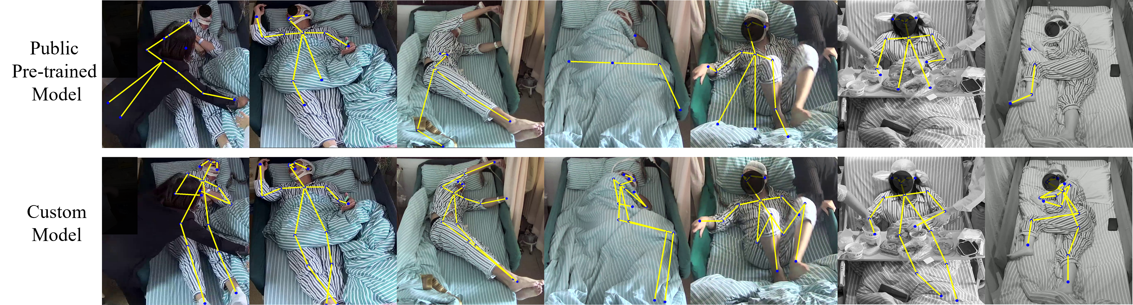
Figure 7: Pose estimation performance comparison between public pre-trained model and our custom model.

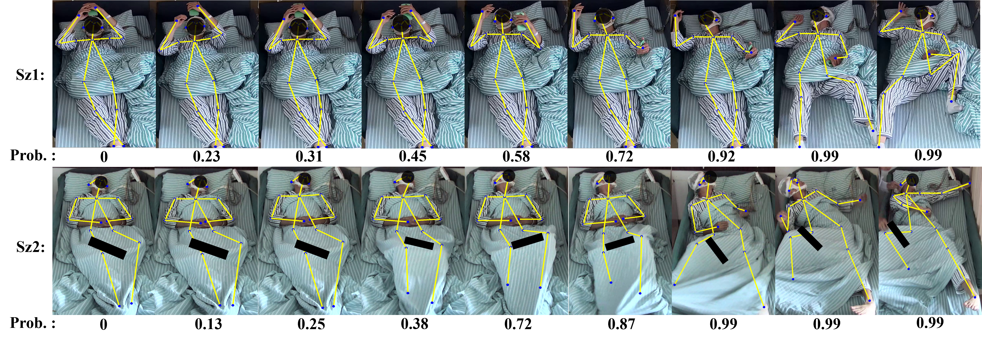
Figure 8: Predictive probabilities of video clips from two different seizures by STViG model. Each frame represents the end frame of the video clip. These frames are not successive. Some subtle changes and eye movements happen during the seizure beginning, but we have to mask the face due to patient information privacy. The black masks are used to follow anonymous and data privacy rules.

PatID

Age

Sex

Type

# seizure

Sen.

FDR

$DT$= 0.5 w/o AP

$DT$= 0.2 w/o AP

$DT$= 0.5 w. AP

$DT$= 0.2 w. AP

$L_{EO}$

$L_{CO}$

$L_{EO}$

$L_{CO}$

$L_{EO}$

$L_{CO}$

$L_{EO}$

$L_{CO}$

pat01

28

M

PG

2

2/2

0

11.5$s$

-1.7$s$

11$s$

-2.2$s$

11.6$s$

-1.7$s$

1.3$s$

-12$s$

pat02

37

M

PG

2

2/2

0

44$s$

-6.2$s$

41.7$s$

-8.5$s$

22.2$s$

-28$s$

20.7$s$

-31.5$s$

pat03

39

M

PG

2

2/2

0

4.5$s$

-1.7$s$

4$s$

-2.2$s$

4.7$s$

-1.5$s$

3$s$

-3.2$s$

pat04

33

F

P

1

1/1

0

27$s$

-4.5$s$

23.5$s$

-8$s$

15.5$s$

-16$s$

12.5$s$

-19$s$

pat05

35

F

PG

3

3/3

0

16.5$s$

-3.6$s$

16$s$

-4.1$s$

15.5$s$

-4.6$s$

5.1$s$

-15$s$

pat06

30

M

P

3

3/3

0

2.2$s$

-0.5$s$

1.7$s$

-1$s$

2.7$s$

0$s$

1.7$s$

-1$s$

pat07

32

M

PG

2

2/2

0

34$s$

-6$s$

32$s$

-8$s$

15$s$

-25$s$

8$s$

-32$s$

pat08

57

F

P

3

3/3

0

7$s$

-1.6$s$

6$s$

-2.6$s$

6.1$s$

-2.5$s$

2$s$

-6.6$s$

pat09

31

M

P

3

3/3

0

6.3$s$

-1.3$s$

6.1$s$

-1.5$s$

5.5$s$

-2.1$s$

5.5$s$

-2.1$s$

pat10

24

F

P

2

2/2

0

4.2$s$

-1$s$

3.7$s$

-1.5$s$

4.2$s$

-1$s$

3.2$s$

-1.9$s$

pat11

55

F

P

3

3/3

0

11.5$s$

-2.6$s$

11$s$

-3.1$s$

11.1$s$

-3$s$

5$s$

-8.1$s$

pat12

23

M

P

4

4/4

0

5$s$

-1.1$s$

4.2$s$

-1.9$s$

5.9$s$

-0.2$s$

4$s$

-2.1$s$

pat13

29

F

PG

1

1/1

0

5$s$

-0.5$s$

0.5$s$

-5$s$

0.5$s$

-5$s$

0.5$s$

-5$s$

pat14

18

M

PG

2

2/2

0

57$s$

-9.7$s$

49.2$s$

-17.5$s$

36$s$

-30.7$s$

16$s$

-50.7$s$

Table 8: Detailed seizure detection performance per patient. M: Male, F: Female, Sen.: Sensitivity (# detected seizure / # total seizure), FDR: False Detection Rate, DT: Decision Threshold, AP: Accumulative Probability strategy, P: Partial seizures, PG: Partial to Generalized seizures.

F. Data usage and availability

The data acquired from the hospital is approved by the Institutional Review Board between us and hospital. We will release the patient video dataset for open access when the sensitive information removal and confidential authorization are finished. Additionally, for the following researcher’s convenience, associated with raw videos, we will also release our trained pose estimation model based on [29] for tracking patient poses in an openpose-based keypoint template.

References

- Andriluka et al. [2014] Mykhaylo Andriluka, Leonid Pishchulin, Peter Gehler, and Bernt Schiele. 2d human pose estimation: New benchmark and state of the art analysis. In Proceedings of the IEEE Conference on computer Vision and Pattern Recognition, pages 3686–3693, 2014.
- Bazarevsky et al. [2020] Valentin Bazarevsky, Ivan Grishchenko, Karthik Raveendran, Tyler Zhu, Fan Zhang, and Matthias Grundmann. Blazepose: On-device real-time body pose tracking. arXiv preprint arXiv:2006.10204, 2020.
- Cao et al. [2017] Zhe Cao, Tomas Simon, Shih-En Wei, and Yaser Sheikh. Realtime multi-person 2d pose estimation using part affinity fields. In CVPR, 2017.
- Cao et al. [2019] Z. Cao, G. Hidalgo Martinez, T. Simon, S. Wei, and Y. A. Sheikh. Openpose: Realtime multi-person 2d pose estimation using part affinity fields. IEEE TPAMI, 2019.
- Chen et al. [2021] Yuxin Chen, Ziqi Zhang, Chunfeng Yuan, Bing Li, Ying Deng, and Weiming Hu. Channel-wise topology refinement graph convolution for skeleton-based action recognition. In ICCV, pages 13359–13368, 2021.
- Cuppens et al. [2012] Kris Cuppens, Chih-Wei Chen, Kevin Bing-Yung Wong, Anouk Van de Vel, Lieven Lagae, Berten Ceulemans, Tinne Tuytelaars, Sabine Van Huffel, Bart Vanrumste, and Hamid Aghajan. Using spatio-temporal interest points (stip) for myoclonic jerk detection in nocturnal video. In IEEE EMBC, pages 4454–4457, 2012.
- Dang et al. [2021] Lingwei Dang, Yongwei Nie, Chengjiang Long, Qing Zhang, and Guiqing Li. Msr-gcn: Multi-scale residual graph convolution networks for human motion prediction. In ICCV, pages 11467–11476, 2021.
- Duan et al. [2022a] Haodong Duan, Jiaqi Wang, Kai Chen, and Dahua Lin. Dg-stgcn: dynamic spatial-temporal modeling for skeleton-based action recognition. arXiv preprint arXiv:2210.05895, 2022a.
- Duan et al. [2022b] Haodong Duan, Yue Zhao, Kai Chen, Dahua Lin, and Bo Dai. Revisiting skeleton-based action recognition. In CVPR, pages 2969–2978, 2022b.
- Fang et al. [2022] Hao-Shu Fang, Jiefeng Li, Hongyang Tang, Chao Xu, Haoyi Zhu, Yuliang Xiu, Yong-Lu Li, and Cewu Lu. Alphapose: Whole-body regional multi-person pose estimation and tracking in real-time. IEEE TPAMI, 2022.
- Feichtenhofer [2020] Christoph Feichtenhofer. X3d: Expanding architectures for efficient video recognition. In CVPR, pages 203–213, 2020.
- Feichtenhofer et al. [2019] Christoph Feichtenhofer, Haoqi Fan, Jitendra Malik, and Kaiming He. Slowfast networks for video recognition. In CVPR, pages 6202–6211, 2019.
- Geertsema et al. [2018] Evelien E Geertsema, Roland D Thijs, Therese Gutter, Ben Vledder, Johan B Arends, Frans S Leijten, Gerhard H Visser, and Stiliyan N Kalitzin. Automated video-based detection of nocturnal convulsive seizures in a residential care setting. Epilepsia, 59:53–60, 2018.
- Han et al. [2022] Kai Han, Yunhe Wang, Jianyuan Guo, Yehui Tang, and Enhua Wu. Vision gnn: An image is worth graph of nodes. NeurIPS, 35:8291–8303, 2022.
- Han et al. [2023] Yan Han, Peihao Wang, Souvik Kundu, Ying Ding, and Zhangyang Wang. Vision hgnn: An image is more than a graph of nodes. In ICCV, pages 19878–19888, 2023.
- He et al. [2016] Kaiming He, Xiangyu Zhang, Shaoqing Ren, and Jian Sun. Deep residual learning for image recognition. In CVPR, pages 770–778, 2016.
- Hussein et al. [2018] Ramy Hussein, Hamid Palangi, Rabab Ward, and Z Jane Wang. Epileptic seizure detection: A deep learning approach. arXiv preprint arXiv:1803.09848, 2018.
- Ji et al. [2012] Shuiwang Ji, Wei Xu, Ming Yang, and Kai Yu. 3d convolutional neural networks for human action recognition. IEEE TPAMI, 35(1):221–231, 2012.
- Kalitzin et al. [2012] Stiliyan Kalitzin, George Petkov, Demetrios Velis, Ben Vledder, and Fernando Lopes da Silva. Automatic segmentation of episodes containing epileptic clonic seizures in video sequences. IEEE TBME, 59(12):3379–3385, 2012.
- Karácsony et al. [2022] Tamás Karácsony, Anna Mira Loesch-Biffar, Christian Vollmar, Jan Rémi, Soheyl Noachtar, and João Paulo Silva Cunha. Novel 3d video action recognition deep learning approach for near real time epileptic seizure classification. Scientific Reports, 12(1):19571, 2022.
- Kong and Fu [2022] Yu Kong and Yun Fu. Human action recognition and prediction: A survey. International Journal of Computer Vision, 130(5):1366–1401, 2022.
- Li et al. [2019a] Guohao Li, Matthias Muller, Ali Thabet, and Bernard Ghanem. Deepgcns: Can gcns go as deep as cnns? In CVPR, pages 9267–9276, 2019a.
- Li et al. [2019b] Maosen Li, Siheng Chen, Xu Chen, Ya Zhang, Yanfeng Wang, and Qi Tian. Actional-structural graph convolutional networks for skeleton-based action recognition. In CVPR, pages 3595–3603, 2019b.
- Lin et al. [2014] Tsung-Yi Lin, Michael Maire, Serge Belongie, James Hays, Pietro Perona, Deva Ramanan, Piotr Dollár, and C Lawrence Zitnick. Microsoft coco: Common objects in context. In Computer Vision–ECCV 2014: 13th European Conference, Zurich, Switzerland, September 6-12, 2014, Proceedings, Part V 13, pages 740–755. Springer, 2014.
- Liu et al. [2020] Ziyu Liu, Hongwen Zhang, Zhenghao Chen, Zhiyong Wang, and Wanli Ouyang. Disentangling and unifying graph convolutions for skeleton-based action recognition. In CVPR, pages 143–152, 2020.
- Liu et al. [2021] Zhenguang Liu, Haoming Chen, Runyang Feng, Shuang Wu, Shouling Ji, Bailin Yang, and Xun Wang. Deep dual consecutive network for human pose estimation. In CVPR, pages 525–534, 2021.
- Moshé et al. [2015] Solomon L Moshé, Emilio Perucca, Philippe Ryvlin, and Torbjörn Tomson. Epilepsy: new advances. The Lancet, 385(9971):884–898, 2015.
- Munir et al. [2023] Mustafa Munir, William Avery, and Radu Marculescu. Mobilevig: Graph-based sparse attention for mobile vision applications. In CVPR, pages 2210–2218, 2023.
- Osokin [2018] Daniil Osokin. Real-time 2d multi-person pose estimation on cpu: Lightweight openpose. In arXiv preprint arXiv:1811.12004, 2018.
- Shi et al. [2019] Lei Shi, Yifan Zhang, Jian Cheng, and Hanqing Lu. Two-stream adaptive graph convolutional networks for skeleton-based action recognition. In CVPR, pages 12026–12035, 2019.
- Shi et al. [2020] Lei Shi, Yifan Zhang, Jian Cheng, and Hanqing Lu. Skeleton-based action recognition with multi-stream adaptive graph convolutional networks. IEEE TIP, 29:9532–9545, 2020.
- Shoeb and Guttag [2010] Ali H Shoeb and John V Guttag. Application of machine learning to epileptic seizure detection. In ICML, pages 975–982, 2010.
- Song et al. [2020] Yi-Fan Song, Zhang Zhang, Caifeng Shan, and Liang Wang. Stronger, faster and more explainable: A graph convolutional baseline for skeleton-based action recognition. In ACM MM, pages 1625–1633, 2020.
- Tang et al. [2021] Siyi Tang, Jared A Dunnmon, Khaled Saab, Xuan Zhang, Qianying Huang, Florian Dubost, Daniel L Rubin, and Christopher Lee-Messer. Self-supervised graph neural networks for improved electroencephalographic seizure analysis. arXiv preprint arXiv:2104.08336, 2021.
- Thijs et al. [2019] Roland D Thijs, Rainer Surges, Terence J O’Brien, and Josemir W Sander. Epilepsy in adults. The Lancet, 393(10172):689–701, 2019.
- Thodoroff et al. [2016] Pierre Thodoroff, Joelle Pineau, and Andrew Lim. Learning robust features using deep learning for automatic seizure detection. In Proceedings of the 1st Machine Learning for Healthcare Conference, pages 178–190. PMLR, 2016.
- Toshev and Szegedy [2014] Alexander Toshev and Christian Szegedy. Deeppose: Human pose estimation via deep neural networks. In Proceedings of the IEEE conference on computer vision and pattern recognition, pages 1653–1660, 2014.
- Tran et al. [2015] Du Tran, Lubomir Bourdev, Rob Fergus, Lorenzo Torresani, and Manohar Paluri. Learning spatiotemporal features with 3d convolutional networks. In ICCV, pages 4489–4497, 2015.
- Tran et al. [2018] Du Tran, Heng Wang, Lorenzo Torresani, Jamie Ray, Yann LeCun, and Manohar Paluri. A closer look at spatiotemporal convolutions for action recognition. In CVPR, pages 6450–6459, 2018.
- Tzallas et al. [2012] Alexandros T Tzallas, Markos G Tsipouras, Dimitrios G Tsalikakis, Evaggelos C Karvounis, Loukas Astrakas, Spiros Konitsiotis, and Margaret Tzaphlidou. Automated epileptic seizure detection methods: a review study. Epilepsy–Histological, Electroencephalographic and Psychological Aspects, pages 2027–2036, 2012.
- van der Lende et al. [2016] Marije van der Lende, Fieke M. E. Cox, Gerhard H. Visser, Josemir W. Sander, and Roland D. Thijs. Value of video monitoring for nocturnal seizure detection in a residential setting. Epilepsia, 2016.
- van Westrhenen et al. [2020] Anouk van Westrhenen, George Petkov, Stiliyan N Kalitzin, Richard HC Lazeron, and Roland D Thijs. Automated video-based detection of nocturnal motor seizures in children. Epilepsia, 61:S36–S40, 2020.
- Wu et al. [2023] Jiafu Wu, Jian Li, Jiangning Zhang, Boshen Zhang, Mingmin Chi, Yabiao Wang, and Chengjie Wang. Pvg: Progressive vision graph for vision recognition. In ACM MM, pages 2477–2486, 2023.
- Xu et al. [2024] Yankun Xu, Jie Yang, Wenjie Ming, Shuang Wang, and Mohamad Sawan. Shorter latency of real-time epileptic seizure detection via probabilistic prediction. Expert Systems with Applications, 236, 2024.
- Yan et al. [2018] Sijie Yan, Yuanjun Xiong, and Dahua Lin. Spatial temporal graph convolutional networks for skeleton-based action recognition. In AAAI, 2018.
- Yang et al. [2021] Yonghua Yang, Rani A. Sarkis, Rima El Atrache, Tobias Loddenkemper, and Christian Meisel. Video-based detection of generalized tonic-clonic seizures using deep learning. IEEE JBHI, 2021.
- Yue et al. [2022] Rujing Yue, Zhiqiang Tian, and Shaoyi Du. Action recognition based on rgb and skeleton data sets: A survey. Neurocomputing, 2022.
- Zeiler and Fergus [2013] Matthew D Zeiler and Rob Fergus. Visualizing and understanding convolutional networks, 2013.
- Zhang et al. [2023] Bo Zhang, YunPeng Tan, Zheng Zhang, Wu Liu, Hui Gao, Zhijun Xi, and Wendong Wang. Factorized omnidirectional representation based vision gnn for anisotropic 3d multimodal mr image segmentation. In ACM MM, pages 1607–1615, 2023.