A Sparse Factor Model for Clustering High-Dimensional Longitudinal Data

Abstract

Recent advances in engineering technologies have enabled the collection of a large number of longitudinal features. This wealth of information presents unique opportunities for researchers to investigate the complex nature of diseases and uncover underlying disease mechanisms. However, analyzing such kind of data can be difficult due to its high dimensionality, heterogeneity and computational challenges. In this paper, we propose a Bayesian nonparametric mixture model for clustering high-dimensional mixed-type (e.g., continuous, discrete and categorical) longitudinal features. We employ a sparse factor model on the joint distribution of random effects and the key idea is to induce clustering at the latent factor level instead of the original data to escape the curse of dimensionality. The number of clusters is estimated through a Dirichlet process prior. An efficient Gibbs sampler is developed to estimate the posterior distribution of the model parameters. Analysis of real and simulated data is presented and discussed. Our study demonstrates that the proposed model serves as a useful analytical tool for clustering high-dimensional longitudinal data.
Keywords: Bayesian nonparametric model; Clustering; High dimensional data; Longitudinal data; Mixture model

1 Introduction

In medical studies, longitudinal data are typically collected from the same individual or a group of individuals at multiple time points, allowing for the examination of changes and patterns over time. Recent advances in engineering technologies have enabled the collection of large amounts of high-dimensional longitudinal data. This type of data refers to data that consists of measurements or observations taken over time on a large number of features or outcomes. Examples include longitudinal and high dimensional multi-omic data (Sailani et al.,, 2020), imaging data (Zipunnikov et al.,, 2014) and physical and cognitive status data (Bruce et al.,, 1994). These features can be of different types, including continuous, discrete, categorical, or mixed-type, and can come from multiple sources such as high throughput sequencing, electronic health records and administrative databases. This wealth of information presents unique opportunities for researchers to investigate the complex nature of diseases and uncover underlying disease phenotypes. However, analyzing such data can be difficult due to their high dimensionality, heterogeneity and computational challenges. Statistical and machine learning methods for handling high dimensional longitudinal data have been emerging, for example, generalized estimation equations (Wang et al.,, 2012), linear mixed effect model (An et al.,, 2013; Li et al.,, 2018), test of significance (Fang et al.,, 2020), variable selection (Fu et al.,, 2021), supervised learning (Adhikari et al.,, 2019; Capitaine et al.,, 2021).

Although few methods are developed for clustering high-dimensional longitudinal data, there is a considerable amount of literature on clustering longitudinal data with low-dimensional features (also known as multi-dimensional longitudinal data) (Lu et al., 2023a, ). Examples include group-based multi-trajectory analysis (Nagin et al.,, 2018), K-means clustering (Genolini et al.,, 2013; Bruckers et al.,, 2016), Hierarchical clustering (Zhou et al.,, 2023), non-parametric clustering (Lv et al.,, 2020), model-based clustering using mixed effect models (Marshall et al.,, 2006; Villarroel et al.,, 2009; Proust-Lima et al.,, 2017) functional clustering(Jacques and Preda,, 2014; Bouveyron and Jacques,, 2011; Lim et al.,, 2020), Bayesian mixture models (Neelon et al.,, 2011; Lu and Lou,, 2021, 2022; Tan et al.,, 2022; Lu et al., 2023b, ), and hidden Markov models (Xia and Tang,, 2019), etc. These methods have been investigated only under a small number of features and their performance and scalability to the high dimensional setting have not been investigated. In particular, Yang and Wu, (2022) proposed a model-based clustering method for high-dimensional longitudinal data via regularisation, and Sun et al., (2017) proposed a Dirichlet process mixture model for clustering longitudinal gene expression data. However, the former approach focuses on fixed and random effects selection on covariates while considering one single longitudinal outcome, while the latter approach requires the longitudinal gene data measured at a set of fixed time points that are identical between individuals.

In this paper, we aim to address this methodological gap by developing a novel Bayesian nonparametric mixture model for clustering high-dimensional, irregularly sampled and mixed-type longitudinal features. The proposed model assumes that the high-dimensional longitudinal data being collected are error-prone measurements of an unobserved low-dimensional set of latent variables (known as latent factors), and the key idea is to induce clustering at the latent factor level instead of the original data to escape the curse of dimensionality. The proposed model is appealing in several aspects: (a) the proposed model allows clustering of mixed-type (e.g., continuous, discrete and categorical) longitudinal features that are measured at irregular time points, (b) the number of measurements can differ between features and between individuals, (c) the number of clusters does not need to be specified a priori and is estimated from the model with a Dirichlet process prior, (d) an efficient Gibbs sampler is developed to estimate the posterior distributions of the model parameters.

The rest of the paper is organized as follows: Section 2 describes the proposed Bayesian non-parametric mixture model for high dimensional longitudinal data. Section 3 describes the Bayesian inference of the model parameters. Section 4 utilizes two case studies to demonstrate the utility of the proposed model. Section 5 describes a simulation study to demonstrate the proposed model’s performance compared to possible competing methods. Finally, Section 6 discusses our findings and future direction.

2 Methods

In this section, we first briefly describe the latent factor model for clustering high dimensional cross-sectional data and then describe the proposed latent factor mixture for clustering high dimensional longitudinal data.

2.1 Latent factor mixture model

The LAtent factor Mixture model for Bayesian clustering (lamb) originally proposed to cluster high-dimensional continuous data assuming that the intrinsic dimension of the data is small (Chandra et al.,, 2023). Specifically, the lamb assumes that the high dimensional data being collected provide error-prone measurements of an unobserved low-dimensional set of latent variables (known as latent factors), and the clustering is performed at the latent factor level instead of the original data to achieve parsimony.

Let $\bm{y}_{i}=(y_{i1},...,y_{ip})^{\top}$ be a $p$-dimensional continuous response variables, for $i=1,...,N$. A class of latent factor mixture models is defined as $\bm{y}_{i}\sim f(\bm{y}_{i};\bm{\eta}_{i},\phi)$ and $\bm{\eta}_{i}\sim\sum_{h=1}^{\infty}\pi_{h}g(\bm{\eta}_{i};\bm{\theta}_{h})$, where $\bm{\eta}_{i}=(\eta_{i1},...,\eta_{id})^{\top}$ are $d$ dimensional latent variables. Also, $d<N$ and is assumed to be unknown. The $f(\bm{y}_{i};\bm{\eta}_{i},\phi)$ is the density of the observed data conditional on the latent variables and parameter $\phi$. In addition, $g(\bm{\eta}_{i};\bm{\theta}_{h})$ is a $d$-dimensional kernel density with parameters $\bm{\theta}_{h}$, and $\bm{\eta}_{i}$ carries information of $\bm{y}_{i}$ at a lower dimensional space. The number of factors with non-negligible loadings is viewed as the active number of factors within each cluster.

As a canonical example, one can consider a Gaussian model with a mixture of Gaussians for the latent factor (Chandra et al.,, 2023), i.e.,

$$\bm{y}_{i}\sim\text{MVN}_{p}(\bm{\Lambda}\bm{\eta}_{i},\Sigma),\quad\bm{\eta}_{i}\sim\sum_{h=1}^{\infty}\pi_{h}\text{MVN}_{d}(\bm{\mu}_{h},\bm{\Delta}_{h}),\quad\pi_{h}\sim Q_{0}$$ (1)

where $\text{MVN}_{p}$() denotes a $p$ dimensional multivariate normal distribution, $\bm{\Sigma}=\text{diag}(\sigma^{2}_{1},...,\sigma^{2}_{p})$ is a $p\times p$ diagonal matrix, $\bm{\Lambda}$ is a $p\times d$ matrix of factor loadings and $\bm{\theta}_{h}=(\bm{\mu}_{h},\bm{\Delta}_{h})$, where $\bm{\mu}_{h}$ and $\bm{\Delta}_{h}$ are mean and variance-covariance matrix of the multivariate normal distribution.

2.2 Latent factor mixture for clustering high dimensional longitudinal data

In this subsection, we extend the lamb model to the longitudinal data setting. Let $\bm{y}_{ir}=(y_{ir1},...,y_{irn_{ir}})^{\top}$ denote the measurements for the $i$th individual and $r$th feature, where $i=1,...,N$ and $r=1,...,R$. Also, $n_{ir}$ is the number of measurements which can differ between $i$ and feature $r$. To account for different types of longitudinal features (i.e., continuous, discrete and categorical), we assume the $f_{r}(\bm{y}_{ir}|\bm{\gamma}_{r},\bm{\beta}_{ir})$ is a distribution with a dispersion parameter $\vartheta_{r}$ and the fully specified mean function given by

$$h^{-1}_{r}(E(\bm{y}_{ir}|\bm{\beta}_{ir},\bm{\gamma}_{r}))=\bm{\xi}_{ir}=\bm{x}_{ir}^{\top}\bm{\gamma}_{r}+\bm{Z}_{ir}^{\top}\bm{\beta}_{ir}$$ (2)

where $h_{r}^{-1}$ is an element-wise canonical link function for the mean of the feature $r$. For example, an identify link function can be used for continuous data following Gaussian distribution, a log link function can be used for count data following Poisson distribution and a logit link can be used for binary data following Binomial distribution. The model also involves dispersion parameters $\vartheta_{r}=\sigma^{2}_{r}$, for Gaussian distribution. The corresponding dispersion parameters $\vartheta_{r}$ for Binomial and Poisson distributions are 1. Also, $\bm{x}_{ir}=(\bm{x}_{ir1},...,\bm{x}_{irp_{r}})^{\top}$ is a $p_{r}\times n_{ir}$ design matrix for fixed effect covariates, where $\bm{x}_{irm}=(x_{irm1},...,x_{irmn_{ir}})^{\top}$ for $m=1,...,p_{r}$, where $p_{r}$ is the dimension of the fixed effect covariates. In practice, each longitudinal feature may share the same set of fixed effect covariates, and in such a case, $p_{1}=p_{2}=...=p_{R}=p$. Furthermore, $\bm{\gamma}_{r}$ is the corresponding vector of coefficients, $\bm{Z}_{ir}$ is a $q_{r}\times n_{ir}$ design matrix for random effect covariates (e.g., time or age), and $\bm{\beta}_{ir}=(\beta_{ir1},...,\beta_{irq_{r}})^{\top}$ is the corresponding random effect coefficients, where $q_{r}$ is the dimension of the random effect for feature $r$. For identification reasons, we assume that the vectors $\bm{x}_{ir}$ and $\bm{Z}_{ir}$ do not contain the same covariates. This specification is similar to the model proposed by Komárek and Komárková, (2013).

To model the dependence within and between features, we assume a joint distribution between random effects estimated from different features. Specifically, let $\bm{\beta}_{i}=(\bm{\beta}_{i1}^{\top},...,\bm{\beta}_{iR}^{\top})^{\top}$ be the joint vector of random effect for all $R$ features of individual $i$. To induce clustering, one could propose to directly perform clustering on $\bm{\beta}_{i}$. However, the dimension of the joint random effect $\bm{\beta}_{i}$ grows rapidly with the number of features $R$ increasing and the dimension of the random effect $q_{r}$ for each feature $r$ increasing. This could cause an unstable model due to the curse of dimensionality. To mitigate this problem, we consider a sparse factor model (Bhattacharya and Dunson,, 2011) on $\bm{\beta}_{i}$, in which the factor loading $\bm{\eta}_{i}$ is assumed to come from an infinite mixture model. Thus, the latent factor mixture model for the joint random effects is

$$\bm{\beta}_{i}\sim\text{MVN}_{q}(\bm{\Lambda}\bm{\eta}_{i},\bm{\Sigma}_{\beta}),\quad\bm{\eta}_{i}\sim\sum_{h=1}^{\infty}\pi_{h}\text{MVN}_{d}(\bm{\mu}_{h},\bm{\Delta}_{h}),\quad\pi_{h}\sim Q_{0}$$ (3)

where $\bm{\Lambda}$ is a $q\times d$ factor loadings matrix with $d<q$, $\bm{\eta}_{i}=(\eta_{i1},...,\eta_{id})^{\top}$ is a $d$-dimensional latent factor for individual $i$, and $\bm{\Sigma}_{\beta}=\text{diag}(\omega_{\beta 1}^{2},...,\omega_{\beta q}^{2})$. Equivalently, the model can be written as $\bm{\beta}_{i}=\bm{\Lambda}\bm{\eta}_{i}+\bm{\epsilon}_{i},\quad\text{with}\quad\bm{\epsilon}_{i}\sim\text{MVN}_{q}(\bm{0},\bm{\Sigma}_{\beta})$, where $\bm{\epsilon}_{i}=(\epsilon_{i1},...,\epsilon_{iq})^{\top}$, for $i=1,...,N$, is a residual vector that is independent with the other variables in the model and is normally distributed with mean zero and a diagonal covariance matrix $\bm{\Sigma}_{\beta}$. In practice, the latent factor dimension $d$ is unknown and needs to be set. In the current study, we choose the smallest $d$ (denoted by $\widehat{d}$) which explains at least 95% of the random effect obtained from mixed effect models. The $\widehat{d}$ can be found using methods such as principal component analysis. A sketch of the proposed model framework is described in Figure 1.

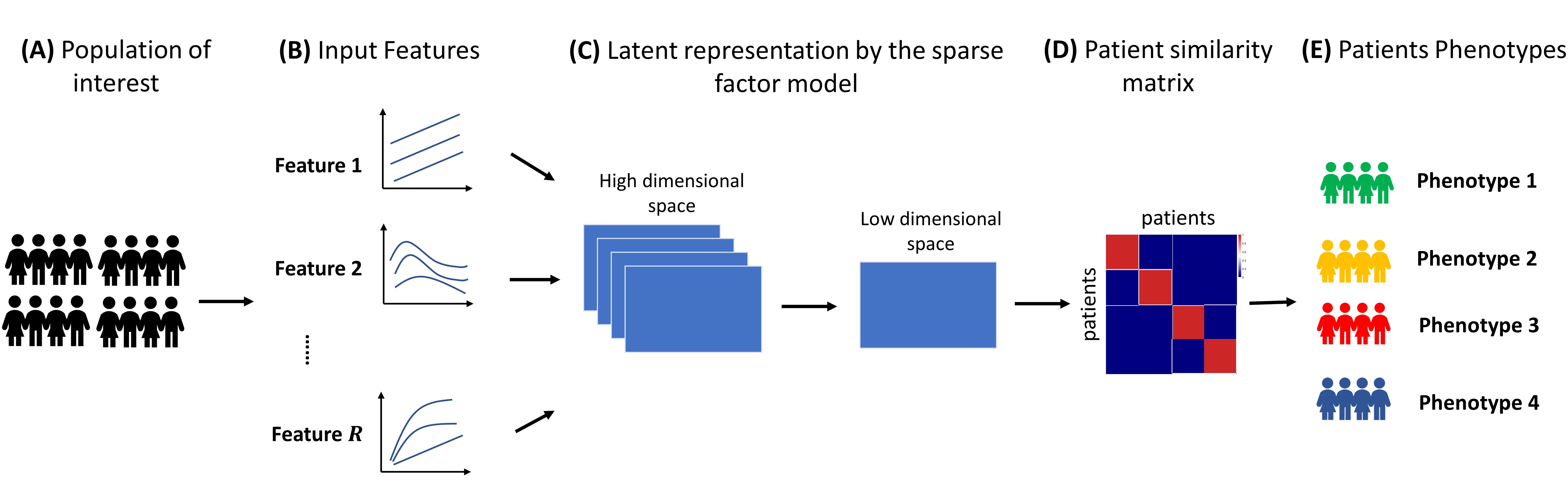
Figure 1: Diagram of the proposed mixture of factor model for high-dimensional longitudinal data

3 Bayesian Inference

In this section, we describe the specification of prior distributions for the proposed model and sketch the computation steps for the posterior distribution.

3.1 Specification of the prior distributions

Given the dimensionality, choosing conditionally conjugate priors that lead to efficient posterior computation via blocked Gibbs sampling is important. Here, we complete our proposed model by describing the specification of the prior distributions for model parameters.

To induce shrinkage and reduce dimensionality, a Dirichlet-Laplace prior (Bhattacharya et al.,, 2015) with parameter $a$ is used. Specifically, we let $\text{vec}(\bm{\Lambda})\sim\text{DL}(a)$. Equivalently, let $\lambda_{kh}$ denote the element of $\bm{\Lambda}$ in the $k^{th}$ row and $h^{th}$ column, for $k=1,...,q$ and $h=1,..,d$, the hierarchal form the prior can be written as

$$\lambda_{kh}|\cdot\sim\text{N}(0,\varphi_{kh}\phi^{2}_{kh}\tau^{2}),\quad\varphi_{kh}\sim\text{Exp}(1/2),\quad\phi_{kh}\sim\text{Dir}(a,...,a),\quad\tau\sim\text{Gamma}(qda,1/2)$$ (4)

where $\text{Exp}(a)$ is an exponential distribution with mean $1/a$, $\text{Dir}(a,...,a)$ is the $q$ dimensional Dirichlet distribution, and $\text{Gamma}(a,b)$ is a gamma distribution with mean $a/b$ and variance $a/b^{2}$. In addition, for the diagonal elements of $\bm{\Sigma}_{\beta}$, we set $\omega_{\beta k}^{-2}\sim\text{Gamma}(a_{\omega},b_{\omega})$, for $k=1,...,q$. For residual variance $\sigma^{2}_{r}$, we set $\sigma^{-2}_{r}\sim\text{Gamma}(a_{\sigma,r},b_{\sigma,r})$, for $r=1,...,R$. For the cluster weight $\pi_{h}$, for $h=1,...,\infty$, we use a stick-breaking prior from a Dirichlet process, which has concentration parameter $\alpha$ impacting the induced prior on the number of clusters. A recent study shows that the consistency for the number of clusters in the Dirichlet process mixtures can be achieved if the concentration parameter is adapted in a fully Bayesian way (Ascolani et al.,, 2023). The hierarchical model defined in (3) for $\bm{\eta}_{i}$ can be represented as

$$\bm{\eta}_{i}|\bm{\mu}_{i},\bm{\Delta}_{i}\sim\text{MVN}_{d}(\bm{\mu}_{i},\bm{\Delta}_{i}),\quad\bm{\mu}_{i},\bm{\Delta}_{i}|G\sim G,\quad G\sim\text{DP}(\alpha,G_{0}),\quad\alpha\sim\text{Gamma}(a_{\alpha},b_{\alpha})$$ (5)

where the base distribution $G_{0}=\text{NIW}(\bm{\mu}_{0},\bm{\Delta}_{0},\kappa_{0},\nu_{0})$, where $\bm{\mu}_{0}$ and $\bm{\Delta}_{0}$ are mean vector and inverse scale matrix, respectively, $\kappa_{0}$ and $\nu_{0}$ are precision parameter and degree of freedom, respectively.

3.2 Posterior computation

To obtain the posterior distribution of model parameters, we developed a Gibbs sampling algorithm with a split-merge update (Jain and Neal,, 2004). The split-merge update allows the algorithm to escape local modes and therefore resulting in an appropriate clustering of individuals. The detailed steps of sampling model parameters are described in Section A of the supplementary material. Convergence of the algorithm is diagnosed using visual inspection of trace plots and the Geweke statistics (Geweke,, 1991). The Geweke statistics determines whether a Markov chain convergence or not based on a test for equality of the means of the first and last part of a Markov chain (by default the first 10% and the last 50%). If the samples are drawn from the stationary distribution of the chain, the two means are equal and Geweke’s statistic has an asymptotically standard normal distribution.

3.3 Inference of clusters

In the mixture model, a well-known issue is the label-switching problem. This problem arises because the likelihood function of the model is invariant to the re-parametrization of the cluster labels. Due to this issue, the cluster labels and the cluster-specific parameters are not identifiable through posterior inference. However, the posterior probability of two individual $i$ and $j$ assigning to the same clusters $P(c_{i}=c_{j}|\bm{Y})$ is identifiable, where $c_{i}$ denotes the cluster label for individual $i$ and $\bm{Y}$ denotes data from all individuals. Using this approach, we first define a distance metric $\widetilde{d}(i,j)=1-P(c_{i}=c_{j}|\bm{Y})$, which reflects the probability of individual $i$ and $j$ not being assigned to the same cluster, and therefore it measures the dissimilarity between the two individuals. $\widetilde{d}(i,j)$ can be estimated by $\sum_{s=1}^{S}I(c_{i}=c_{j})$, where $S$ is the number of MCMC iterations. A $N\times N$ posterior similarity matrix is constructed with $\widetilde{d}(i,j)$ as its $(i,j)$ element. Then the clustering is obtained by minimizing the posterior expectation of the Binders loss function (Binder,, 1978) .

4 Application

In this section, we apply the proposed model to two real-life examples to demonstrate its utility. The first dataset concerns analyzing high dimensional longitudinal cytokines data to identify distinct biological patterns for individuals living in California while the second dataset concerns identifying disease phenotypes of Primary Biliary Cholangitis (PBC) patients based on mix-typed biomarkers.

4.1 Example 1: Longitudinal Cytokine Data

4.1.1 Data description

The data come from a study of multi-omics seasonal patterns for a group of healthy individuals living in California (Sailani et al.,, 2020). The original cohort includes longitudinal multi-omics data from profiling 105 individuals aged 25 to 75 years old. The data from this cohort includes quarterly sample collections of transcriptomes from peripheral blood mononuclear cells, proteome and metabolome from plasma and targeted cytokine and growth factor assays using serum. In total, there were 902 visits (average across different types of omics) from which samples were collected over up to 4 years. These samples were then aggregated and mapped to a 1-year-long time frame (Sailani et al.,, 2020). The sample collections were generally evenly distributed throughout the year. However, the measurement time points and frequencies differed between participants (Figure 2A). In addition, participants in this study were characterized for steady-state plasma glucose (SSPG), in which 31 participants were insulin sensitive (SSPG $<$ 150 mg/dL), and 35 were insulin resistant (SSPG $\geq$ 150 mg/dL).

In the current analysis, we included 61 participants who have cytokine (immune protein) data. Cytokines are a broad category of small proteins that play a crucial role in cell signaling. They are primarily produced by immune cells and are involved in coordinating immune responses and regulating various biological processes in the body. Among the included participants, 27 (44.3%) were insulin sensitive (IS) and 34 (55.7%) were insulin resistant (IR) individuals (insulin resistance is often associated with Type 2 diabetes). The goal of the analysis is to identify individuals’ subgroups based on 66 longitudinal cytokines. The full list of variable names is provided in Table S1. All cytokines were log-transformed prior to the cluster analysis. The individual trajectories of two selected cytokines (IL17F and MCSF) over time are shown in Figure 2B and Figure 2C, respectively. Subsequently, to further characterize the resulting clusters, we associated the clusters with individuals’ insulin status.

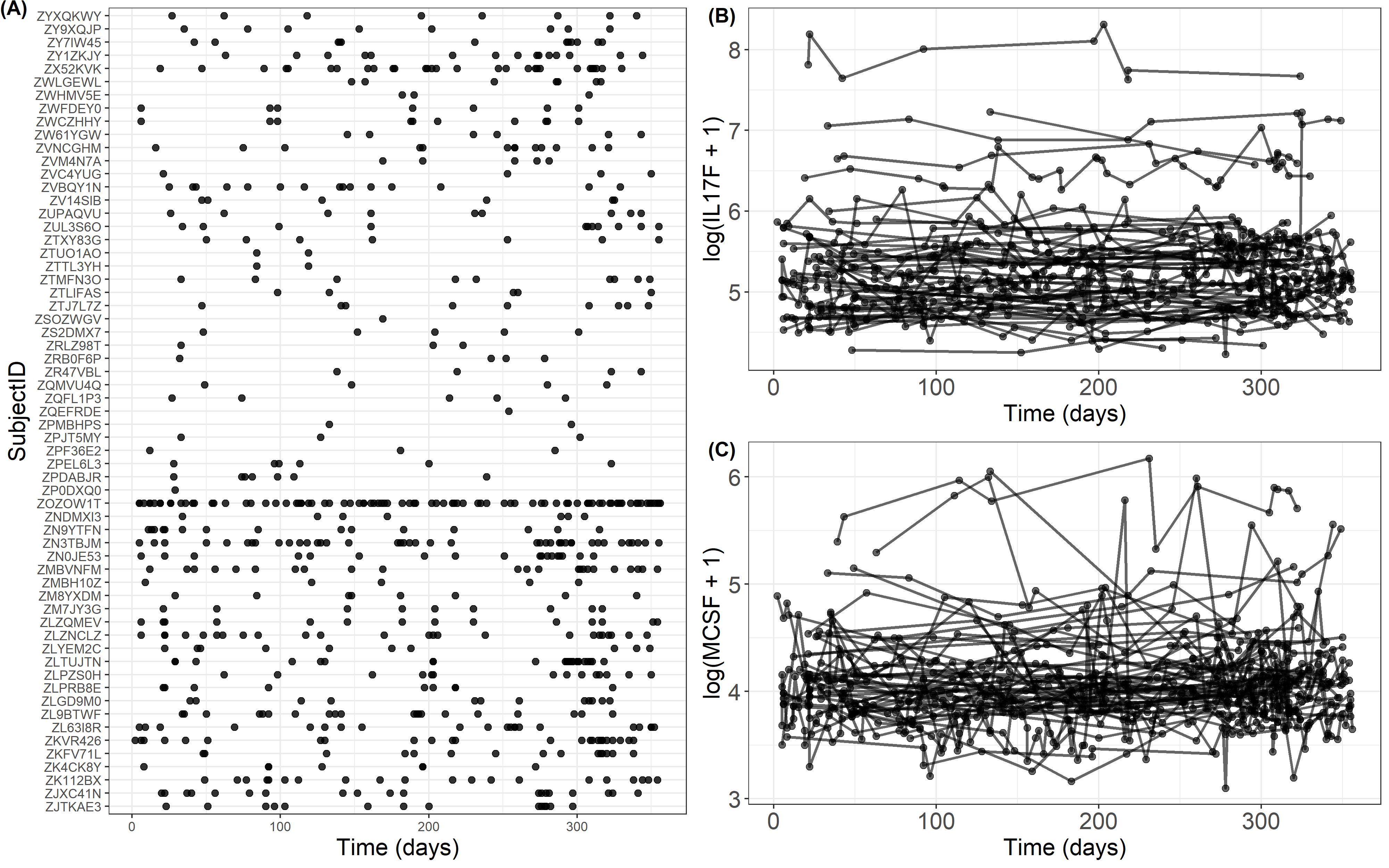
Figure 2: Observed time grid for longitudinal immune protein data by individual ID and longitudinal trajectories of two selected immune protein markers for the longitudinal cytokines data (Example 1). (A) Observed time grid of each individual in the longitudinal immune protein data. (B) Longitudinal trajectory of IL17F in log scale. (C) Longitudinal trajectory of MCSF in log scale.

4.1.2 Model specification

For this application, hyperparameters were set to reflect weak prior information for the model parameters. Specifically, following a previous study (Bhattacharya et al.,, 2015), we set $a=0.5$ for the Dirichlet-Laplace prior distribution. Also, we set $a_{\sigma,r}=b_{\sigma,r}=0.01$, $a_{\omega,r}=b_{\omega,r}=0.01$ for $r=1,...,R$. For the concentration parameter, we considered four different scenarios, namely (a) $a_{\alpha}=b_{\alpha}=0.1$, reflecting a weakly informative prior (Figure 3A), (b) $a_{\alpha}=b_{\alpha}=1$, reflecting a weakly to moderately informative prior (Figure 3B), (c) $a_{\alpha}=b_{\alpha}=10$, reflecting a moderately to strongly informative prior (Figure 3C), and (d) $a_{\alpha}=b_{\alpha}=50$, reflecting a strongly informative prior (Figure 3D). For the base distribution $G_{0}$, we set $\bm{\mu}_{0}=\bm{0}$, $\bm{\Delta}$ to be a diagonal matrix with elements being 80, $\nu_{0}=116$ and $\kappa=0.001$.

To allow sufficient flexibility and to fully capture the dependence between markers and measurements within individuals, a linear form random effects of time (i.e., both random intercept and slope) was used, i.e., we set $\bm{Z}_{ir}=(1,{t}_{ir})^{\top}$, where ${t}_{ir}=(t_{i1},...,t_{in_{i}})^{\top}$. This resulted in a dimension of 132 for random effect $\bm{\beta}_{i}$. In addition, the model is adjusted for a baseline covariate BMI, i.e., $\bm{x}_{ir}=(\text{BMI}_{ir})^{\top}$ for $r=1,...,R$. We ran the model with 20000 iterations, discarded the first 10000 samples and kept every 10th sample. This resulted in 1000 samples for each model parameter.

Next, we used leave-one-out cross-validation to investigate the cluster stability. We created 61 subsets from the original data by holding out 1 individual (Hennig,, 2007). We refit the proposed model based on this subset and compared the results (both the estimated number of clusters and the individual cluster membership) to those obtained from the original data. The agreement between the two clusterings was measured using the adjusted rand index (aRand) (Hubert and Arabie,, 1985). A higher aRand suggests a better agreement between the two clusterings under evaluation.

4.1.3 Analysis results

The clustering results based on the model under different values of concentration parameter $\alpha$ for the Dirichlet process prior are shown in Figure 3. The trace plots for $\alpha$ showed that all models were mixing well (Figure S1). All models consistently identified two clusters (Figure 3E, F, G and H) and the clusterings were quite stable even for extreme choice of prior hyperparameters, for example, $\alpha\sim\text{Gamma}(0.1,0.1)$ and $\alpha\sim\text{Gamma}(50,50)$, suggesting that the resulting clustering uncovered the underlying heterogeneity that may reflect a biological difference among these individuals. The distribution of the clusters differed slightly under different prior of $\alpha$ (Figure 3I, J, K, L). For example, when $\alpha\sim\text{Gamma}(0.1,0.1)$, 7 (11%) individuals were assigned to Cluster 1 while 54 (89%) individuals were assigned to Cluster 2. When $\alpha\sim\text{Gamma}(50,50)$, 12 (20%) individuals were assigned to Cluster 1 while 49 (80%) individuals were assigned to Cluster 2. The resulting clusters showed distinct prevalence in individuals’ insulin status, further suggesting biological differences between the clusters (Figure 3M, N,O, P). For example, under the model with $\alpha\sim\text{Gamma}(0.1,0.1)$, all 7 individuals (100%) from Cluster 1 were insulin sensitive whereas only 20( 37%) individuals from Cluster 2 were insulin sensitive. Under the model with $\alpha\sim\text{Gamma}(50,50)$, 9 (75%) individuals from Cluster 1 were insulin sensitive whereas only 18 (36.7%) individuals from Cluster 2 were insulin sensitive. The leave-one-out validation showed that the median number of clusters over 61 data subsets was around 2 for all models (Figure 4A) while the model with $\alpha\sim\text{Gamma}(50,50)$ yielded slightly higher aRand, suggesting clustering were more stable compared to other models.

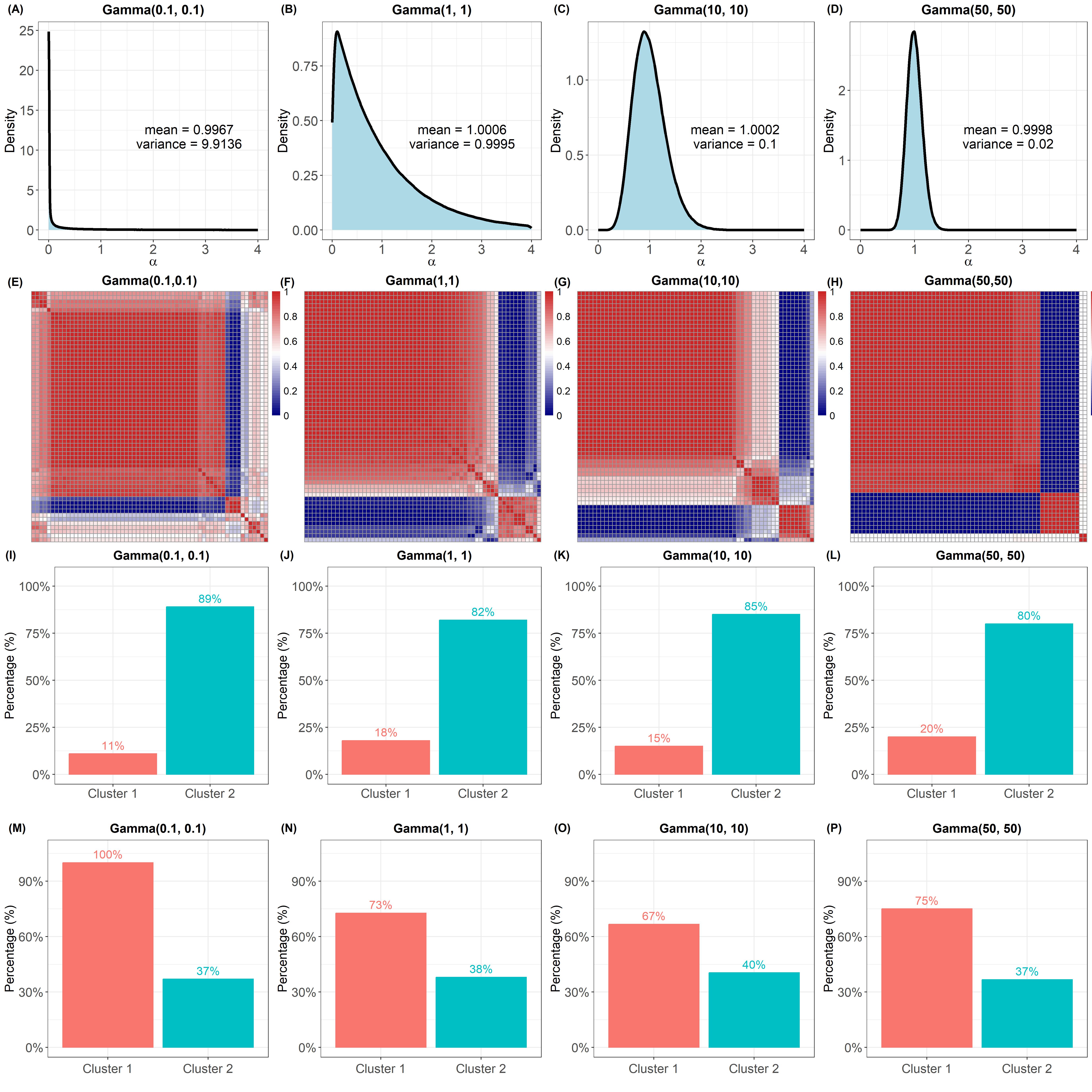
Figure 3: Prior distributions for the concentration parameter $\alpha$, Posterior similarity matrix, the cluster proportions and the prevalence of insulin resistance by clusters for the longitudinal cytokines data (Example 1). (A) Prior distribution for $\alpha\sim\text{Gamma}(0.1,0.1)$. (B) Prior distribution for $\alpha\sim\text{Gamma}(1,1)$. (C) Prior distribution for $\alpha\sim\text{Gamma}(10,10)$. (D) Prior distribution for $\alpha\sim\text{Gamma}(50,50)$. (E) Posterior similarity matrix for $\alpha\sim\text{Gamma}(0.1,0.1)$. (F) Posterior similarity matrix for $\alpha\sim\text{Gamma}(1,1)$. (G) Posterior similarity matrix for $\alpha\sim\text{Gamma}(10,10)$. (H) Posterior similarity matrix for $\alpha\sim\text{Gamma}(50,50)$. (I) Cluster proportions based on $\alpha$ under prior $\text{Gamma}(0.1,0.1)$. (J) Cluster proportions based on $\alpha$ under prior $\text{Gamma}(1,1)$. (K) Cluster proportions based on $\alpha$ under prior $\text{Gamma}(10,10)$. (L) Cluster proportions based on $\alpha$ under prior $\text{Gamma}(50,50)$. (M) Proportion of insulin-sensitive individuals by clusters from the model with $\alpha\sim\text{Gamma}(0.1,0.1)$. (N) Proportion of insulin-sensitive individuals by clusters from the model with $\alpha\sim\text{Gamma}(1,1)$. (O) Proportion of insulin-sensitive individuals by clusters from the model with $\alpha\sim\text{Gamma}(10,10)$. (P) Proportion of insulin-sensitive individuals by clusters from the model with $\alpha\sim\text{Gamma}(50,50)$.

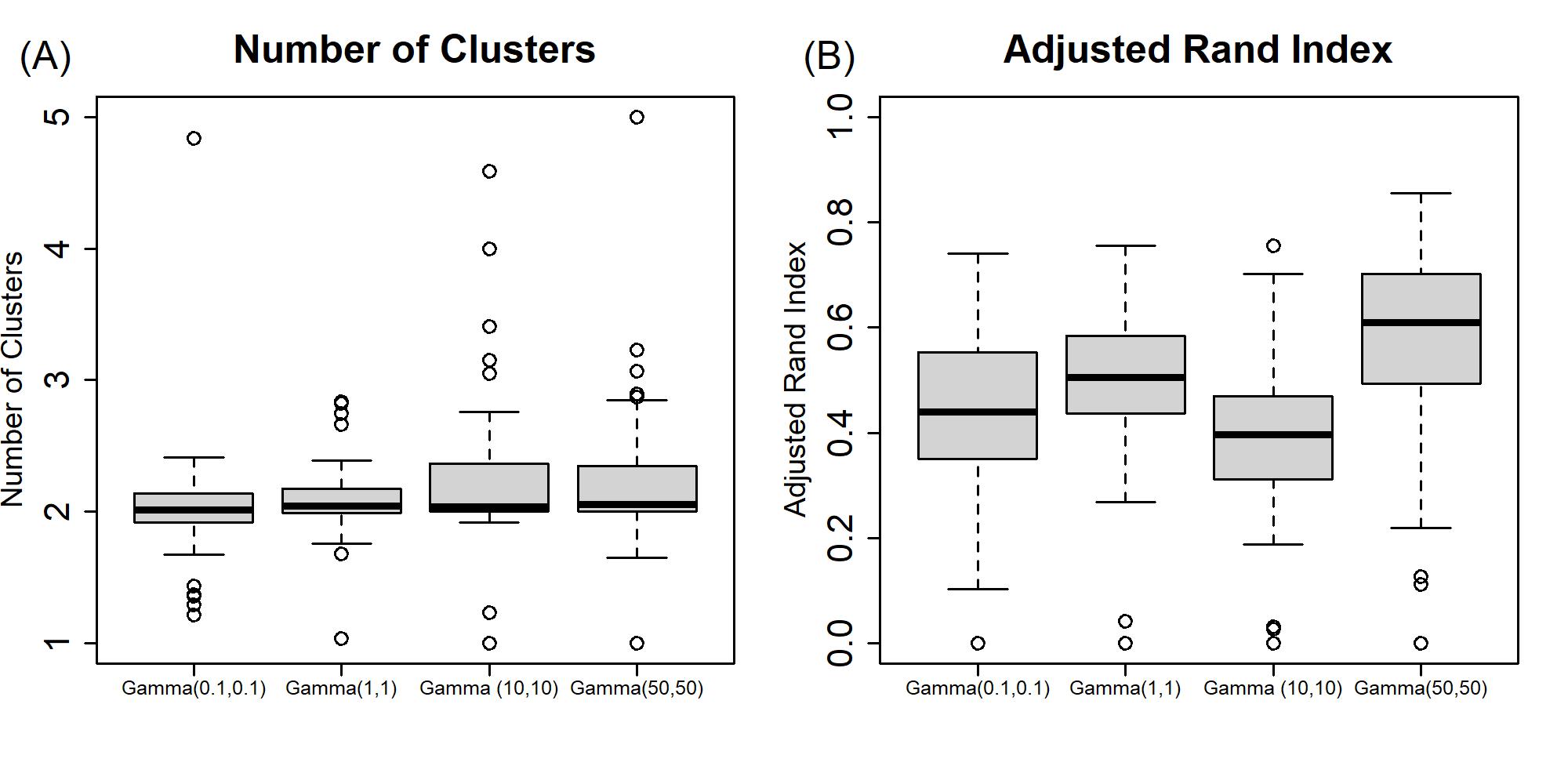
Figure 4: Stability of the number of clusters and individual cluster membership over 61 data subsets under different prior for $\alpha$ for the longitudinal cytokines data (Example 1). (A) Distribution of the estimated number of clusters by prior distributions of $\alpha$. (B) Distribution of the adjusted Rand index by prior distributions of $\alpha$.

4.2 Example 2: Primary Biliary Cholangitis Data

4.2.1 Data description

Primary Biliary Cholangitis (PBC) is a chronic liver disease with an unknown cause. A randomized placebo-controlled trial of the drug D-penicillamine for PBC patients was conducted between 1974 and 1984 (Dickson et al.,, 1989). During the study, multiple longitudinal markers were collected to monitor patients’ disease progress, example variables include serum albumin, alkaline phosphotase, presence of ascites and serum bilirubin. The data are available at http://lib.stat.cmu.edu/datasets/pbcseq. Consistent with previous studies (Komárek and Komárková,, 2013; Lu and Lou,, 2022), we only include $N=260$ patients known to be alive at 910 days (30 months) of follow-up, and the longitudinal measurements up to this point.

The goal of the current analysis was to identify patients’ subgroups based on 10 longitudinal (continuous or categorical) biological markers, namely (1) presence of ascites (ascites), (2) presence of hepatomegaly or enlarged liver (hepatom), (3) the presence of blood vessel malformations in the skin (spiders), (4) presence of edema (edema.bin), (5) log of serum bilirunbin (mg/dl) (lbili), (6) log of serum albumin (g/dl) (lalbumin), (7) log of alkaline phosphotase (U/liter) (lalk.phos), (8) log of serum glutamic-oxaloacetic transaminase (lsgot), (9) log of platelet count (lplatelet), (10) log of standardized blood clotting time. Subsequently, to further characterize the resulting clusters, we associated the clusters with the survival status after 30 months using Kaplan-Meier analysis. Time to death was considered as an event of interest and liver transplantation was considered as censoring.

4.2.2 Model specification

We used the same specification hyper-parameters except we set $\nu_{0}=50$ and $\bm{\Delta}$ to be a diagonal matrix with elements being 100. Similarly, to allow sufficient flexibility and to fully capture the dependence between markers and measurements within individuals, a linear form of random effects of time (i.e., both random intercept and slope) was used. This resulted in a dimension of 20 for random effect $\bm{\beta}_{i}$. In addition, the model adjusted for baseline age and sex. We ran the model with 20000 iterations, discarded the first 10000 samples and kept every 10th sample. This resulted in 1000 samples for each model parameter.

To evaluate the cluster stability, cross-validation was used by creating 50 subsets from the original data by holding out 10 or 11 individuals. We refit the proposed model based on this subset and compared the results (both the estimated number of clusters and the individual cluster membership) to those obtained from the original data. Similarly, aRand was used to measure the agreement between the two clusterings.

4.2.3 Analysis results

For all models, the trace plots of MCMC samples suggested the model converged well (Figure S2). The clustering results based on the model under different prior distributions for $\alpha$ are shown in Figure S3. In general, the number of clusters and the size of the clusters differ between models under different prior distributions for $\alpha$. Specifically, when $\alpha\sim\text{Gamma}(0.1,0.1)$, two clusters were obtained (Figure S3A), with Cluster 1 accounting for 63.8% of patients and Cluster 2 accounting for 36.2% patients, respectively. Markers such as hepatom, spiders, edema.bin and lbili showed distinct patterns between the two clusters while others such as lalbumin, lalk.phos, lchol, lsogt, lplatelet and lprotime appeared to be similar between clusters (Figure S4). This suggested that patients belonging to Cluster 1 were more likely to have a presence of hepatomegaly or enlarged liver (hepatom), blood vessel malformations in the skin (spiders), presence of edema (edema.bin), and higher value of serum bilirunbin (mg/dl) (lbili). Therefore, Cluster 1 represented a group of patients with worse conditions and significantly lower survival probabilities after 30 months of follow-up, compared to Cluster 2 (Figure S3E). When $\alpha\sim\text{Gamma}(1,1)$, three clusters were obtained (Figure S3B), with Cluster 1 accounting for 35.4% of patients, Cluster 2 accounting for 26.5% patients and Cluster 3 accounting for 38.1% patients, respectively. The markers that were separated among clusters were also hepatom, spiders, edema.bin and lbili (Figure S5). Clusters 1, 2 and 3 represented patients that had mild, moderate and severe conditions reflected by their survival probabilities after 30 months (Figure S3F). However, the difference between Clusters 2 and 3 in survival probabilities was less evident. When $\alpha\sim\text{Gamma}(10,10)$, three clusters were obtained (Figure S3C), with Cluster 1 accounting for 25.8% of patients, Cluster 2 accounting for 33.5% patients and Cluster 3 accounting for 40.8% patients, respectively. The markers that were separated among clusters were also hepatom, spiders, edema.bin and lbili (Figure S6). Similarly, Clusters 1, 2 and 3 represented patients that had mild, moderate and severe conditions reflected by their survival probabilities after 30 months (Figure S3G). However, the difference between Clusters 1 and 2 in survival probabilities was minimal. When $\alpha\sim\text{Gamma}(50,50)$, three clusters were obtained (Figure S3D), with Cluster 1 accounting for 35.4% of patients, Cluster 2 accounting for 50.8% patients and Cluster 3 accounting for 13.8% patients, respectively. The markers that were separated among clusters were also hepatom, spiders, edema.bin and lbili (Figure S7). Similarly, Clusters 1, 2 and 3 represented patients that had mild, moderate and severe conditions reflected by their survival probabilities after 30 months (Figure S3H). However, the difference between Clusters 2 and 3 in survival probabilities was minimal. The stability of the number of clusters and individual cluster membership under different prior distributions for $\alpha$ over 50 random subsets is shown in Figure S8. A large variation was observed for the number of clusters and the aRand for the prior distribution of $\text{Gamma}(10,10)$ and $\text{Gamma}(50,50)$.

5 Simulation Study

In this section, we perform a simulation study to evaluate the clustering performance of the proposed model under various settings compared to several alternative approaches.

5.1 Simulation setup

Data were generated according to equation (2) with the identity link function. Number of observations was set to be $n_{ir}=6$ for $i=1,...,N$ and $r=1,...,R$. The individual visit time $t_{irj}$ for $r=1,...,R$ and $j=1,...,n_{ir}$ was sampled from a uniform distribution for the intervals of (0, 2), (3, 5), (6, 8), (12, 14), (18, 20), (24, 26), (30, 32) respectively. The number of features that inform clustering structure was set to be $R_{\text{signal}}=3$. For these three features, the random effects (both a random intercept and random slope) were generated from a joint multivariate normal distribution $\text{MVN}(\bm{0},\bm{\Sigma}_{\beta})$. The number of features that were noise (i.e., not informing the clustering structure) was denoted as $R_{\text{noise}}$ and was set to be 25, 50, 75, and 100, respectively. Therefore, the total number of features were $R=R_{\text{signal}}+R_{\text{noise}}$. A time-independent binary covariate was generated from a $\text{Bernouli}(0.5)$ distribution, with fixed effect coefficients set to be -0.5. The number of clusters was set to be $K=2,3,4$, which is commonly seen in clinical practice. The sample size for each cluster was set to be $N_{k}=50$, for $k=1,...,K$. Two different scenarios were considered. In Scenario 1, the patterns of the features informing the clustering structure were relatively constant over time with a slope near zero (Figure S9) while in Scenario 2, a non-zero slope was added to the clusters leading to the trajectory pattern being increased or decreased over time (Figure S10).

We compared the proposed model (called lamb_long) to the following four approaches.

• lamb_twostage: in the first stage, a mixed-effect model was fitted for each longitudinal response and the estimates of the random intercepts and slopes were obtained for each individual. In the second stage, lamb model was applied to the joint random effects to obtain the optimal number of clusters and the cluster partition.

• lamb_first: applying lamb model to only the first measurement of each individual.

• lamb_last: applying lamb model to only the last measurement of each individual.

• K-means clustering: K-means clustering for multivariate longitudinal data using the kml3d package (Genolini et al.,, 2013). For this approach, the number of clusters was determined by the built-in Calinski and Harabatz criterion (Genolini et al.,, 2013).

• hierarchical clustering: hierarchical clustering for multivariate longitudinal data using the clusterMLD package (Zhou et al.,, 2023). For this approach, the number of clusters was determined by the built-in Gap statistics (Zhou et al.,, 2023).

For each setting, 50 datasets were generated. To measure the model performance, we calculated the mean and standard deviation (SD) of the estimated number of clusters ($\widehat{K}$) from each model over all the simulated datasets. To evaluate the model performance on recovering the true underlying cluster structure (i.e., partition), we used the aRand (Hubert and Arabie,, 1985) to measure the agreement between the estimated cluster partition and the true cluster partition. To facilitate a fair comparison, the aRands for K-means and hierarchical clustering were calculated based on the true number of clusters $K$ (instead of the estimated one).

5.2 Simulation results

The mean estimated number of clusters and aRand for Scenarios 1 and 2 are plotted in Figures 5 & 6, respectively. For Scenario 1, lamb_long, lamb_first and lamb_last yielded a reasonably well estimate of the number of clusters for different $K$ (Figure 5A) as well as performing well in recovering the true clustering (Figure 5B). The performance of lamb_first and lamb_last was expected given the clustering can be well determined by the first or last measurement of the individuals (Figure S9). On the other hand, lamb_twostage, K-means Hierachical clustering underestimated or overestimated the number of clusters (Figure 5A) and failed to uncover the true underlying clustering structure particularly when the number of noise variable ($R_{noise}$) and $K$ were large. The mean (SD) of the number of clusters and aRand under different $\alpha$ as well as the competing approaches for Scenario 1 are presented in Table S2.

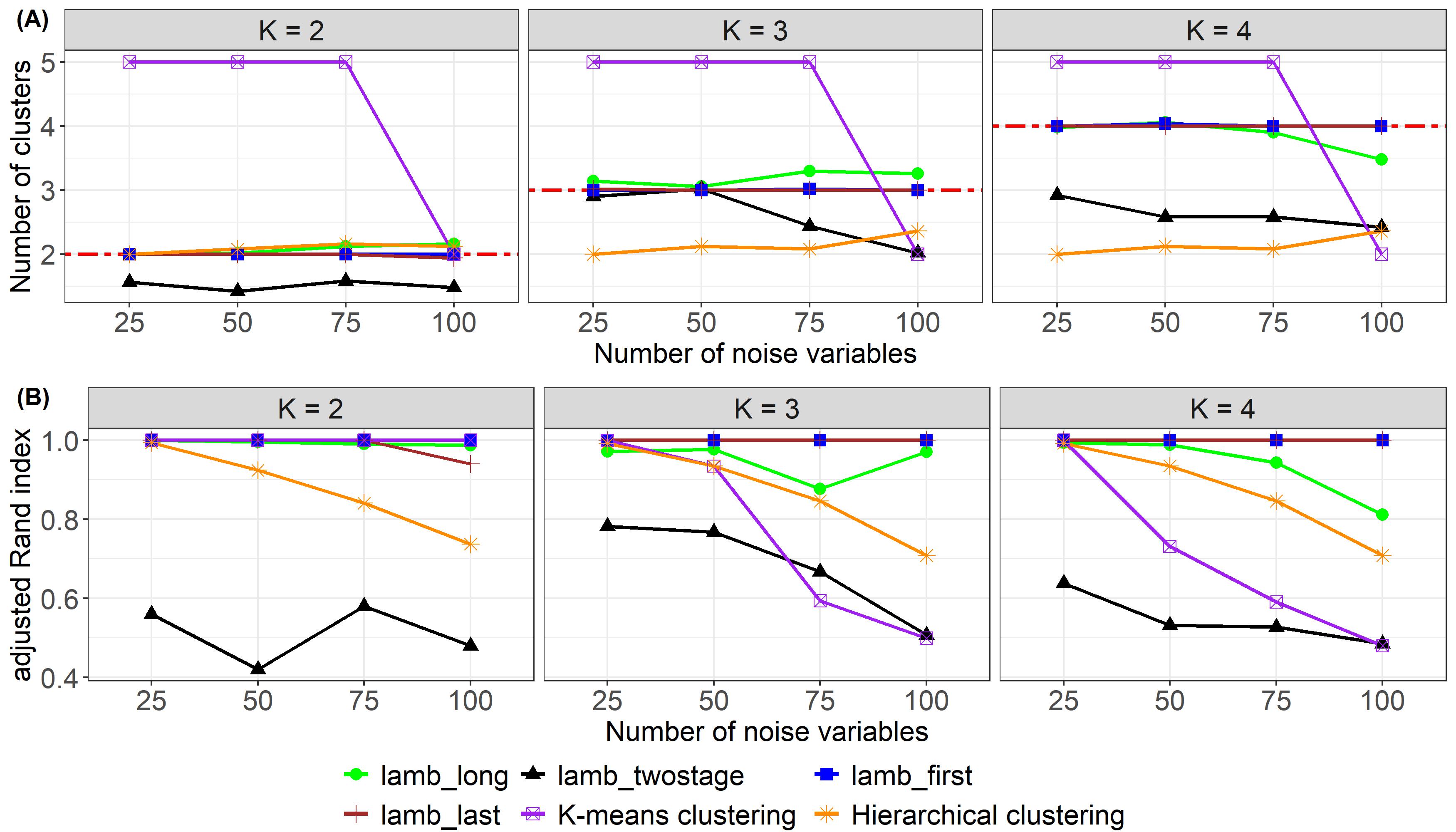
Figure 5: Simulation results for Scenario 1. (A) Mean estimated number of clusters over 50 simulated datasets by methods for $K=$ 2, 3 and 4. The reference line (in red) represents the true number of clusters. (B) Mean adjusted rand index over 50 datasets by methods for $K=$ 2, 3 and 4. lamb_long: lamb for longitudinal data with prior $\alpha\sim\text{Gamma}(0.1,0.1)$. lamb_twostage: lamb for longitudinal data based on a two-stage approach. lamb_first: lamb based on the first measurement of each individual. lamb_first: lamb based on the last measurement of each individual. K-means: K-means clustering for multivariate longitudinal data using kml3d package. Hierarchical clustering: Hierarchical clustering for multivariate longitudinal data using clusterMLD package. For both K-means and Hierarchical clustering, the aRands were calculated under the true number of clusters $K$.

For Scenario 2, lamb_long yielded a reasonably well estimate of the number of clusters for different $K$ (Figure 6A) and performed well in uncovering the true partition (Figure 6B), outperforming the competing approaches most of the time. On the other hand, lamb_twostage, lamb_first and lamb_last underestimated the number of clusters (Figure 6A), leading to poor performance in recovering the true partition (Figure 6B). The K-means and Hierarchical clustering approaches underestimated or overestimated the number of clusters (Figure 6A), particularly when the number of noise variables was large (e.g., $>50$). Given the true number of cluster $K$, the K-means approach performed reasonably well in recovering the true partition when $K=2$ (Figure 6B). However, the K-means approach yielded poor performance when $K=3$ and $K=4$, particularly when $R_{noise}$ is large (e.g., $\geq 50$). The mean (SD) of the number of clusters and aRand under different $\alpha$ as well as the competing approaches for Scenario 2 are presented in Table S3.

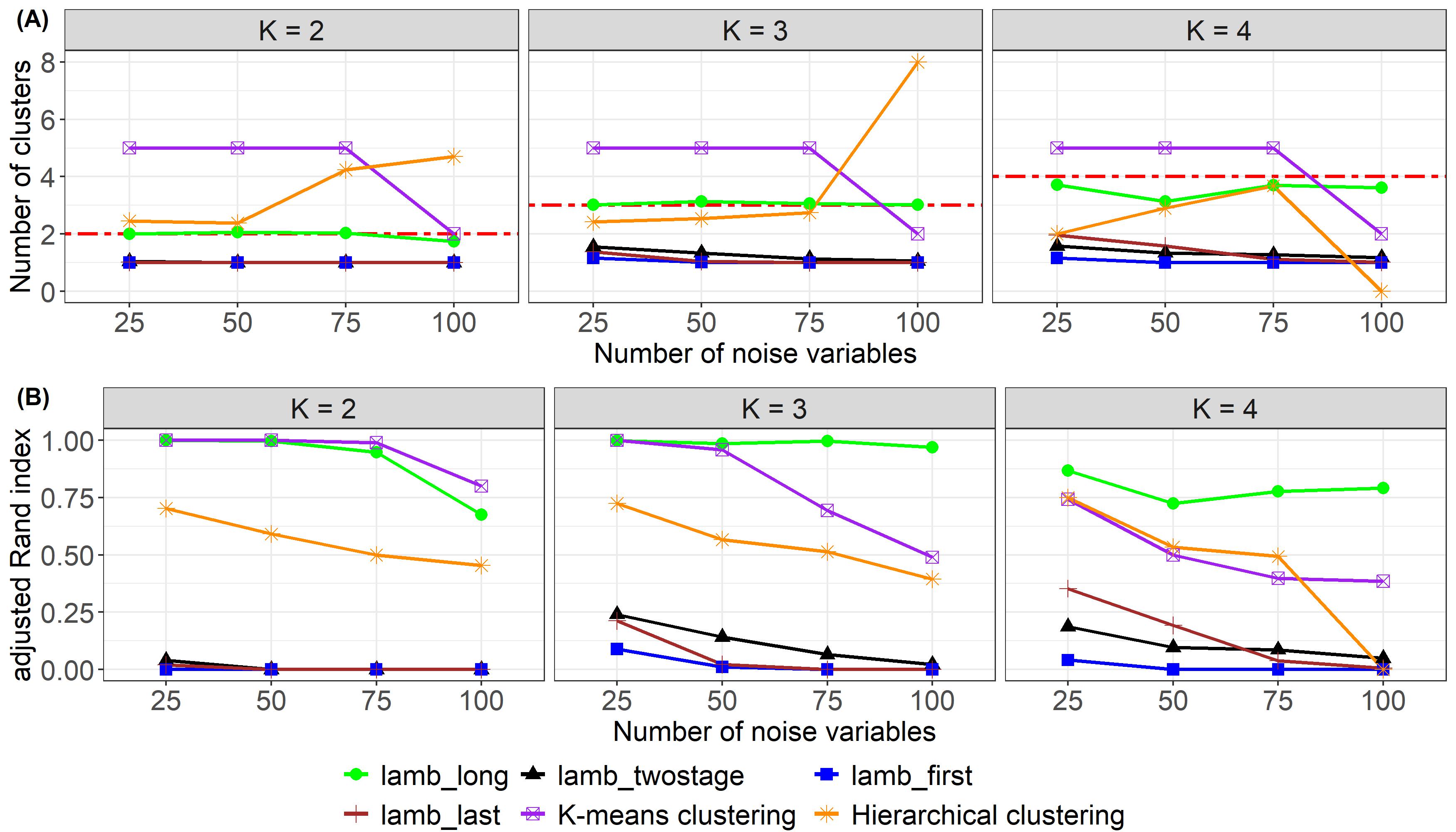
Figure 6: Simulation results for Scenario 2. (A) Mean estimated number of clusters over 50 simulated datasets by methods for $K=$ 2, 3 and 4. The reference line (in red) represents the true number of clusters. (B) Mean adjusted rand index over 50 datasets by methods for $K=$ 2, 3 and 4. lamb_long: lamb for longitudinal data with prior $\alpha\sim\text{Gamma}(0.1,0.1)$. lamb_twostage: lamb for longitudinal data based on a two-stage approach. lamb_first: lamb based on the first measurement of each individual. lamb_first: lamb based on the last measurement of each individual. K-means: K-means clustering for multivariate longitudinal data using kml3d package. Hierarchical clustering: Hierarchical clustering for multivariate longitudinal data using clusterMLD package. For both K-means and Hierarchical clustering, the aRands were calculated under the true number of clusters $K$.

6 Discussion

In the current study, we propose a Bayesian nonparametric model for clustering high-dimensional longitudinal data. The underlying assumptions are that the longitudinal data are correlated within and between features and their dependence can be captured by jointly modeling the random effects, which can be further represented by low-dimensional latent factors.

The proposed model provides a new perspective and an analytical tool for clustering multi-dimensional longitudinal features, as demonstrated through our practical applications and simulation studies. In the cytokines data example, the underlying heterogeneity captured by the proposed model reflects a distinct prevalence of insulin resistance, which suggests a biological difference between the resulting clusters. In the PBC data example, the resulting clusters differed on certain markers but not others, suggesting that not all markers contributed to defining the clusters and it is essential to perform the clustering on a lower dimensional space in which the noise information was removed. This is particularly useful in practice because which features will contribute to the clusterings can be hardly known a priori. Reducing noise and performing the analysis on a lower dimensional space could lead to a more stable and clinically meaningful clustering result. The simulation study demonstrates that the proposed model provides a reasonable well estimation of the number of clusters and the cluster membership under various scenarios with different numbers of clusters and noise features.

There are several directions for future studies. For example, the current model is computed using the Gibbs sampling and split-merge algorithm. To scale up the algorithm to analyze large datasets (e.g., electronic health record data), variational inference can be considered as an alternative (Blei and Jordan,, 2006). In addition, the trajectory can be analyzed through non-parametric functions such as splines to allow for more flexibility in capturing non-linear forms. Finally, our model reduces the dimension of features through latent factors. However, in some clinical settings, determining which variables contribute to the final clustering is of interest, and therefore simultaneously clustering and variable selection (Kim et al.,, 2006) can be considered in future studies.

Nevertheless, the proposed model serves as a useful tool for clustering high-dimensional data with complex data structures and an unknown number of clusters.

Data Availability Statement

The longitudinal cytokine data are available from Sailani et al., (2020) and are hosted on the NIH Human Microbiome 2 project site (https://portal.hmpdacc.org). The PBC data are available from Fleming and Harrington, Appendix D (Fleming and Harrington,, 2013) or in R mixAK package (Komárek et al.,, 2014).

Funding

Z.L. is supported by a Discovery Grant funded by the Natural Sciences and Engineering Research Council of Canada.

References

- Adhikari et al., (2019) Adhikari, S., Lecci, F., Becker, J. T., Junker, B. W., Kuller, L. H., Lopez, O. L., and Tibshirani, R. J. (2019). High-dimensional longitudinal classification with the multinomial fused lasso. Statistics in medicine, 38(12):2184–2205.
- An et al., (2013) An, X., Yang, Q., and Bentler, P. M. (2013). A latent factor linear mixed model for high-dimensional longitudinal data analysis. Statistics in medicine, 32(24):4229–4239.
- Ascolani et al., (2023) Ascolani, F., Lijoi, A., Rebaudo, G., and Zanella, G. (2023). Clustering consistency with dirichlet process mixtures. Biometrika, 110(2):551–558.
- Bhattacharya and Dunson, (2011) Bhattacharya, A. and Dunson, D. B. (2011). Sparse bayesian infinite factor models. Biometrika, pages 291–306.
- Bhattacharya et al., (2015) Bhattacharya, A., Pati, D., Pillai, N. S., and Dunson, D. B. (2015). Dirichlet–laplace priors for optimal shrinkage. Journal of the American Statistical Association, 110(512):1479–1490.
- Binder, (1978) Binder, D. A. (1978). Bayesian cluster analysis. Biometrika, 65(1):31–38.
- Blei and Jordan, (2006) Blei, D. M. and Jordan, M. I. (2006). Variational inference for dirichlet process mixtures. Bayesian analysis, 1(1):121–143.
- Bouveyron and Jacques, (2011) Bouveyron, C. and Jacques, J. (2011). Model-based clustering of time series in group-specific functional subspaces. Advances in Data Analysis and Classification, 5(4):281–300.
- Bruce et al., (1994) Bruce, M. L., Seeman, T. E., Merrill, S. S., and Blazer, D. G. (1994). The impact of depressive symptomatology on physical disability: Macarthur studies of successful aging. American journal of public health, 84(11):1796–1799.
- Bruckers et al., (2016) Bruckers, L., Molenberghs, G., Drinkenburg, P., and Geys, H. (2016). A clustering algorithm for multivariate longitudinal data. Journal of biopharmaceutical statistics, 26(4):725–741.
- Capitaine et al., (2021) Capitaine, L., Genuer, R., and Thiébaut, R. (2021). Random forests for high-dimensional longitudinal data. Statistical methods in medical research, 30(1):166–184.
- Chandra et al., (2023) Chandra, N. K., Canale, A., and Dunson, D. B. (2023). Escaping the curse of dimensionality in bayesian model-based clustering. J. Mach. Learn. Res., 24:144–1.
- Dickson et al., (1989) Dickson, E. R., Grambsch, P. M., Fleming, T. R., Fisher, L. D., and Langworthy, A. (1989). Prognosis in primary biliary cirrhosis: model for decision making. Hepatology, 10(1):1–7.
- Fang et al., (2020) Fang, E. X., Ning, Y., and Li, R. (2020). Test of significance for high-dimensional longitudinal data. Annals of statistics, 48(5):2622.
- Fleming and Harrington, (2013) Fleming, T. R. and Harrington, D. P. (2013). Counting processes and survival analysis, volume 625. John Wiley & Sons.
- Fu et al., (2021) Fu, L., Li, J., and Wang, Y.-G. (2021). Robust approach for variable selection with high dimensional longitudinal data analysis. Statistics in Medicine, 40(30):6835–6854.
- Genolini et al., (2013) Genolini, C., Pingault, J.-B., Driss, T., Côté, S., Tremblay, R. E., Vitaro, F., Arnaud, C., and Falissard, B. (2013). Kml3d: a non-parametric algorithm for clustering joint trajectories. Computer methods and programs in biomedicine, 109(1):104–111.
- Geweke, (1991) Geweke, J. (1991). Evaluating the accuracy of sampling-based approaches to the calculation of posterior moments, volume 196. Federal Reserve Bank of Minneapolis, Research Department Minneapolis, MN, USA.
- Hennig, (2007) Hennig, C. (2007). Cluster-wise assessment of cluster stability. Computational Statistics & Data Analysis, 52(1):258–271.
- Hubert and Arabie, (1985) Hubert, L. and Arabie, P. (1985). Comparing partitions. Journal of classification, 2(1):193–218.
- Jacques and Preda, (2014) Jacques, J. and Preda, C. (2014). Model-based clustering for multivariate functional data. Computational Statistics & Data Analysis, 71:92–106.
- Jain and Neal, (2004) Jain, S. and Neal, R. M. (2004). A split-merge markov chain monte carlo procedure for the dirichlet process mixture model. Journal of computational and Graphical Statistics, 13(1):158–182.
- Kim et al., (2006) Kim, S., Tadesse, M. G., and Vannucci, M. (2006). Variable selection in clustering via dirichlet process mixture models. Biometrika, 93(4):877–893.
- Komárek and Komárková, (2013) Komárek, A. and Komárková, L. (2013). Clustering for multivariate continuous and discrete longitudinal data. The Annals of Applied Statistics, 7(1):177–200.
- Komárek et al., (2014) Komárek, A., Komárková, L., et al. (2014). Capabilities of r package mixak for clustering based on multivariate continuous and discrete longitudinal data. Journal of Statistical Software, 59(12):1–38.
- Li et al., (2018) Li, Y., Wang, S., Song, P. X.-K., Wang, N., Zhou, L., and Zhu, J. (2018). Doubly regularized estimation and selection in linear mixed-effects models for high-dimensional longitudinal data. Statistics and its Interface, 11(4):721.
- Lim et al., (2020) Lim, Y., Cheung, Y. K., and Oh, H.-S. (2020). A generalization of functional clustering for discrete multivariate longitudinal data. Statistical methods in medical research, 29(11):3205–3217.
- (28) Lu, Z., Ahmadiankalati, M., and Tan, Z. (2023a). Joint clustering multiple longitudinal features: A comparison of methods and software packages with practical guidance. Statistics in Medicine, pages 1–28.
- Lu and Lou, (2021) Lu, Z. and Lou, W. (2021). Bayesian approaches to variable selection in mixture models with application to disease clustering. Journal of Applied Statistics, pages 1–21.
- Lu and Lou, (2022) Lu, Z. and Lou, W. (2022). Bayesian consensus clustering for multivariate longitudinal data. Statistics in Medicine, 41(1):108–127.
- (31) Lu, Z., Subbarao, P., and Lou, W. (2023b). A bayesian latent class model for integrating multi-source longitudinal data: application to the child cohort study. Journal of the Royal Statistical Society Series C: Applied Statistics, page qlad100.
- Lv et al., (2020) Lv, Y., Zhu, X., Zhu, Z., and Qu, A. (2020). Nonparametric cluster analysis on multiple outcomes of longitudinal data. Statistica Sinica, 30(4):1829–1856.
- Marshall et al., (2006) Marshall, G., De la Cruz-Mesía, R., Barón, A. E., Rutledge, J. H., and Zerbe, G. O. (2006). Non-linear random effects model for multivariate responses with missing data. Statistics in Medicine, 25(16):2817–2830.
- Nagin et al., (2018) Nagin, D. S., Jones, B. L., Passos, V. L., and Tremblay, R. E. (2018). Group-based multi-trajectory modeling. Statistical methods in medical research, 27(7):2015–2023.
- Neelon et al., (2011) Neelon, B., Swamy, G. K., Burgette, L. F., and Miranda, M. L. (2011). A bayesian growth mixture model to examine maternal hypertension and birth outcomes. Statistics in medicine, 30(22):2721–2735.
- Proust-Lima et al., (2017) Proust-Lima, C., Philipps, V., and Liquet, B. (2017). Estimation of extended mixed models using latent classes and latent processes: the r package lcmm. Journal of Statistical Software, 78(2):1–56.
- Sailani et al., (2020) Sailani, M. R., Metwally, A. A., Zhou, W., Rose, S. M. S.-F., Ahadi, S., Contrepois, K., Mishra, T., Zhang, M. J., Kidziński, Ł., Chu, T. J., et al. (2020). Deep longitudinal multiomics profiling reveals two biological seasonal patterns in california. Nature communications, 11(1):4933.
- Sun et al., (2017) Sun, J., Herazo-Maya, J. D., Kaminski, N., Zhao, H., and Warren, J. L. (2017). A dirichlet process mixture model for clustering longitudinal gene expression data. Statistics in medicine, 36(22):3495–3506.
- Tan et al., (2022) Tan, Z., Shen, C., Subbarao, P., Lou, W., and Lu, Z. (2022). A joint modeling approach for clustering mixed-type multivariate longitudinal data: Application to the child cohort study. arXiv preprint arXiv:2210.08385.
- Villarroel et al., (2009) Villarroel, L., Marshall, G., and Barón, A. E. (2009). Cluster analysis using multivariate mixed effects models. Statistics in medicine, 28(20):2552–2565.
- Wang et al., (2012) Wang, L., Zhou, J., and Qu, A. (2012). Penalized generalized estimating equations for high-dimensional longitudinal data analysis. Biometrics, 68(2):353–360.
- Xia and Tang, (2019) Xia, Y.-M. and Tang, N.-S. (2019). Bayesian analysis for mixture of latent variable hidden markov models with multivariate longitudinal data. Computational Statistics & Data Analysis, 132:190–211.
- Yang and Wu, (2022) Yang, L. and Wu, T. T. (2022). Model-based clustering of high-dimensional longitudinal data via regularization. Biometrics.
- Zhou et al., (2023) Zhou, J., Zhang, Y., and Tu, W. (2023). clustermld: An efficient hierarchical clustering method for multivariate longitudinal data. Journal of Computational and Graphical Statistics, pages 1–14.
- Zipunnikov et al., (2014) Zipunnikov, V., Greven, S., Shou, H., Caffo, B., Reich, D. S., and Crainiceanu, C. (2014). Longitudinal high-dimensional principal components analysis with application to diffusion tensor imaging of multiple sclerosis. The annals of applied statistics, 8(4):2175.