Abstract

We propose an approach to do learning in Gaussian factor graphs. We treat all relevant quantities (inputs, outputs, parameters, latents) as random variables in a graphical model, and view both training and prediction as inference problems with different observed nodes. Our experiments show that these problems can be efficiently solved with belief propagation (BP), whose updates are inherently local, presenting exciting opportunities for distributed and asynchronous training. Our approach can be scaled to deep networks and provides a natural means to do continual learning: use the BP-estimated parameter marginals of the current task as parameter priors for the next. On a video denoising task we demonstrate the benefit of learnable parameters over a classical factor graph approach and we show encouraging performance of deep factor graphs for continual image classification on MNIST.

1 Introduction

Deep learning (DL) has been shown to be effective for solving many scene understanding tasks. However, neural networks (NNs) remain a poor fit in applications where we require efficient, robust representations which can be trained incrementally. An agent with an accurate and continually updating “world model” of its surroundings, including semantic and compositional understanding of objects, is not limited to reactive behaviour, but can attempt novel reasoning via mental simulation  (Stoica:etal:TechReport2017).

Such a world model will probably, at least in the near term, contain various human-created representations and structures, such as an explicit 3D map of a scene. However, it will also need to be able to learn its own abstract representations of complex entities such as objects or movement patterns. The following related properties of its learning mechanism are important:

1. The primary mode of learning should be un- or self-supervised, meaning that a running system can learn useful abstractions without external help.

2. Learning should be continual, taking place incrementally within a running system whose performance is gradually improving in consequence.

3. Learning should run seamlessly alongside existing tried-and-tested hand-designed inference algorithms.

To satisfy desiderata 2 and 3, an agent must be able to fuse multiple models, balancing old vs new, hand-crafted vs learnt. Bayesian inference provides a principle by which multiple signals can be fused: they can be combined according to the rules of probability. The integration of standard DL with incremental probabilistic inference on graphs has so far been with limited success, due to the lack of such principles.

Concurrently, the ability to distribute model training over multiple processing nodes is becoming increasingly important with the growth of i) larger models which must be spread over multiple processors, ii) processors whose cores comprise significant local memory (Graphcore), iii) parallel, distributed and heterogeneous embedded devices (Sutter:Jungle2011). Efficient model-parallel training of NNs with backpropagation is currently limited by backward locking: processors for earlier layers are idle when waiting for the backward error signal. Again, we argue that Bayesian principles provide an answer here: local signals can be fused according to the rules of probability, and this enables effective communication between different regions of a model without relying on a global loss.

Figure 1: In GBP Learning, we design factor graphs whose structure mirrors common neural network architectures, but with learnable parameters included as variables in the graph, and non-linear factors (which have soft-switching behaviour) akin to neurons. The example architecture shown here for image classification comprises a convolutional layer, a max pooling layer and a dense projection layer. A common set of blue parameter variables (circles) is shared across all image/label observations, while there are copies of the red activation and green input/output variables for each observation. Factors (black squares) between layers constrain their representations to be locally consistent, while those attached to inputs and outputs encourage consistency with observations. This example shows a supervised learning setup, but the same architecture could be trained without label supervision by removing the output observation factor. Given such a factor graph, we can train and make predictions in a distributed manner with GBP.

In this paper we propose a new Bayesian approach to machine learning, where parameter learning and communication between layers is part of the same joint procedure. We propose that there is no fundamental difference between traditional “state estimation” via probabilistic inference, and model learning in Bayesian ML. We believe our joint approach to inference and learning distinguishes it from existing methods of Bayesian DL which view them as separate procedures.

Much recent work has shown that Gaussian Belief Propagation (GBP) permits convergent, efficient, incremental inference across a broad range of probabilistic graphical models, including models with non-linear factors and robust cost functions  (Davison:Ortiz:ARXIV2019; Ortiz:etal:CVPR2020; Murai:etal:ARXIV2022; Patwardhan:etal:ARXIV2022). Our hypothesis is that this machinery can be applied to general machine learning, which will take place via inference on large, overparameterised graphs with non-linear Gaussian factors, and architectures resembling common NNs. We call this new approach GBP Learning. We claim that the important features of DL are i) randomly initialised, massively over-parameterised networks (allen2019learning) with ii) architectural motifs which encode good inductive bias, and iii) non-linearities which switch to selectively activate and prune when exposed to data (glorot2011deep) — rather than the specifics of the commonly used backpropagation learning rule. We believe that we can embed these properties in Gaussian factor graphs, while gaining the advantages of probabilistic modelling for continual learning and interfacing with other Bayesian components. Such models can be trained with only local updates using GBP.

Our paper proceeds as follows. First, we briefly describe GBP in Section 2, before introducing our model and how it is trained in Section 3. Experimental results are given in Section 4, before summarising previous work (Section 5) and concluding (Section 6). In short, our contributions are:

1. A new class of deep networks which can be represented as Gaussian factor graphs and trained with BP.

2. Experimental results for convolutional architectures which show promise for continual image classification and video denoising.

2 Background

2.1 Factor graphs

A factor graph is a probabilistic graphical model which defines a joint distribution over variables $\mathbf{X}$ as the product of factors $\Phi=\{\phi_{j}\}$:

$$p\left(\mathbf{X}\right) =\frac{1}{Z}\prod_{j=1}^{|\Phi|}\phi_{j}\left(\mathbf{x}_{\phi_{j}}\right)~{}.$$ (1)

Here $\mathbf{x}_{\phi_{j}}$ denotes the vector of all $V_{j}$ variables in the neighbourhood of $\phi_{j}$ and $Z$ is a normalising constant. A factor graph is bipartite: variables only connect to factors and vice versa. Each factor may encode an observation, or prior about a variable or group of variables. Factor functions $\phi_{j}(\cdot)$ may unnormalised distributions and relate to their energy, $E_{j}(\cdot)$, as

$$\phi_{j}\left(\mathbf{x}_{\phi_{j}}\right) =\exp\left(-E_{j}\left(\mathbf{x}_{\phi_{j}}\right)\right).$$ (2)

A Gaussian factor graph is one in which all $\{E_{j}\}$ are quadratic in the related observation $\mathbf{y}_{j}$, i.e.

$$E_{j}\left(\mathbf{x}_{\phi_{j}}\right)=\frac{1}{2}\left(\mathbf{y}_{j}-\mathbf{h}\left(\mathbf{x}_{\phi_{j}}\right)\right)^{{}^{\top}}{\Lambda_{\mathbf{y}_{j}}}\left(\mathbf{y}_{j}-\mathbf{h}\left(\mathbf{x}_{\phi_{j}}\right)\right)~{},$$ (3)

where $\mathbf{h}\left(\cdot\right)$ is the measurement function, and $\Lambda_{\mathbf{y}_{j}}$ is the measurement precision. Note that $\mathbf{y}_{j}$ may be a “pseudo-observation”, e.g. the mean of a prior on $\mathbf{x}_{\phi_{j}}$.

2.2 Belief Propagation

Belief Propagation (pearl1988probabilistic) is a message passing algorithm which can perform inference on factor graphs via distributed, iterative computation. Each message is passed along the edge between one factor $\phi_{j}$ and one variable $x_{i}$. Messages travel in both directions, and we use the notations $m_{{\phi_{j}\rightarrow x_{i}}}$ and $m_{{x_{i}\rightarrow\phi_{j}}}$ for the two types of message. A message takes the form of a probability distribution in the space of the variable involved. The following update rules are iterated until convergence:

$$m_{{x_{i}\rightarrow\phi_{j}}}\left(x_{i}\right) \leftarrow\prod_{k\in\mathrm{ne}\left(i\right)\setminus j}m_{{\phi_{k}\rightarrow x_{i}}}\left(x_{i}\right)$$ (4)

$$m_{{\phi_{j}\rightarrow x_{i}}}\left(x_{i}\right) \leftarrow\sum_{\{x_{n}\}_{\mathrm{ne}\left(j\right)\setminus i}}\phi_{j}\left(\mathbf{x}_{\phi_{j}}\right)\prod_{n\in\mathrm{ne}\left(j\right)\setminus i}m_{{x_{n}\rightarrow\phi_{i}}}\left(x_{n}\right),$$ (5)

where $\mathrm{ne}\left(i\right)\setminus j$ indicates the indices of all nodes connected to node $i$, except $j$. After convergence the posterior marginal of a variable can be estimated by the product of its incoming messages:

$$p\left(x_{i}\right) =\frac{1}{Z_{i}}\prod_{j\in\mathrm{ne}\left(i\right)}m_{{\phi_{j}\rightarrow x_{i}}}\left(x_{i}\right)~{},$$ (6)

where $Z_{i}$ is straightforward to compute as $p(x_{i})$ is assumed to belong to a known parametric family. In this work, we assume the variable nodes are univariate, but BP can be extended for multivariate posterior inference by passing vector messages between sets of variables and factors. BP updates (4), (5), (6) have a number of interesting properties. First, all the required computations rely only on the local state of the graph; no global context is necessary. Second, by working in terms of natural parameters, taking the product of a set of messages is reduced to the addition of their parameters.

The above routine (4), (5) is guaranteed to converge to the correct marginals in tree-structured graphs but not for graphs containing cycles. Despite a lack of guarantees, application of BP to loopy graphs has been successful in many domains, most notably for error-correcting codes (gallager1962low; mackay1997near).

2.2.1 Gaussian Belief Propagation

In Gaussian factor graphs, messages $m_{{x_{i}\rightarrow\phi_{j}}}\left(x_{i}\right)$ and $m_{{\phi_{j}\rightarrow x_{i}}}\left(x_{i}\right)$ are normal distributions, parameterised by precision (inverse covariance) matrix $\Lambda$ and information vector $\eta$. The products in the variable to factor message formula (4) become sums:

$$\Lambda_{{x_{i}\rightarrow\phi_{j}}} \leftarrow\sum_{k\in\mathrm{ne}\left(i\right)\setminus j}\Lambda_{{\phi_{k}\rightarrow x_{i}}}\left(x_{i}\right)~{};$$ (7)

$$\eta_{{x_{i}\rightarrow\phi_{j}}} \leftarrow\sum_{k\in\mathrm{ne}\left(i\right)\setminus j}\eta_{{\phi_{k}\rightarrow x_{i}}}\left(x_{i}\right).$$

These updates can be implemented efficiently by computing the belief for $x_{i}$ once (6) and then subtracting the incoming message from each factor to get the corresponding outgoing message. For a factor $\phi_{j}$ with precision matrix $\Lambda^{\left(\phi_{j}\right)}\in\mathbb{R}^{V_{j}\times V_{j}}$ and information vector $\eta^{\left(\phi_{j}\right)}\in\mathbb{R}^{V_{j}}$, the factor to variable messages are:

$$\Lambda_{{\phi_{j}\rightarrow x_{i}}} \leftarrow\Lambda^{\left(\phi_{j}\right)}_{i,i}-\Lambda^{\left(\phi_{j}\right)}_{i,\setminus i}\Sigma_{\setminus i,\setminus i}^{\left(\phi_{j}+m\right)}\Lambda^{\left(\phi_{j}\right)}_{\setminus i,i}~{};$$ (8)

$$\eta_{{\phi_{j}\rightarrow x_{i}}} \leftarrow\eta^{\left(\phi_{j}\right)}_{i}-\Lambda^{\left(\phi_{j}\right)}_{i,\setminus i}\Sigma_{\setminus i,\setminus i}^{\left(\phi_{j}+m\right)}\eta^{\left(\phi_{j}+m\right)}_{\setminus i}~{},$$

where we have used $\Sigma_{\setminus i,\setminus i}^{\left(\phi_{j}+m\right)}=\left(\Lambda^{\left(\phi_{j}\right)}_{\setminus i,\setminus i}+\left(\mathbf{D}_{\phi_{j}}\right)_{\setminus i,\setminus i}\right)^{-1}$, $\eta^{\left(\phi_{j}+m\right)}:=\eta^{\left(\phi_{j}\right)}+\mathbf{e}_{\phi_{j}}$, $\mathbf{D}_{\phi_{j}}$ for the matrix of precision messages coming into $\phi_{j}$, and $\mathbf{e}_{\phi_{j}}$ for the vector of incoming information messages. Subscript _∖r indicates all elements except that for variable $r$. Note that $\mathbf{D}_{\phi_{j}}$ is diagonal for graphs with scalar variable nodes.

As in the general case, GBP is not guaranteed to converge in graphs with cycles. However, if it does converge in linear-Gaussian models, it is guaranteed to converge to the correct posterior means(weiss1999correctness). In practice, it has been empirically shown that this correct convergence reliably happens in many types of factor graph. We refer the reader to ortiz2021visual for an in-depth introduction to GBP.

2.3 Non-linear Factors

GBP supports the use of factors which include non-linear transformations of their connected variables, and this is crucial in our proposed use here for representation learning. Every time we compute messages from a non-linear factor, we linearise it around the current estimates of the variables, $\mathbf{X}_{0}$, i.e. for each factor $\mathbf{h}\left(\mathbf{x}_{\phi_{j}}\right)\approx\mathbf{h}\left(\mathbf{x}_{\phi_{j},0}\right)+\mathbf{J}_{j}^{{}^{\top}}\left(\mathbf{x}_{\phi_{j}}-\mathbf{x}_{\phi_{j},0}\right)$ where $\mathbf{J}_{j}:=\left.\frac{\partial\mathbf{h}\left(\mathbf{x}_{\phi_{j}}\right)}{\partial\mathbf{x}_{\phi_{j}}}\right|_{\mathbf{x}_{\phi_{j},0}}$. Linearisation can be implemented using the following forms of factor precision and information in (8):

$$\Lambda^{(\phi_{j})} \approx\mathbf{J}_{j}^{{}^{\top}}\Lambda_{\mathbf{y}_{j}}\mathbf{J}_{j}$$ (9)

$$\eta^{(\phi_{j})} \approx\mathbf{J}_{j}^{{}^{\top}}\Lambda_{\mathbf{y}_{j}}\left(\mathbf{J}_{j}^{{}^{\top}}\mathbf{x}_{\phi_{j},0}+\mathbf{y}_{j}-\mathbf{h}\left(\mathbf{x}_{\phi_{j},0}\right)\right).$$

See Section 3.3 of Davison:Ortiz:ARXIV2019 for details and derivation.

3 GBP Learning

Our aim is to produce factor graphs which share similar architectural inductive biases to NNs, that can be overparameterised in a similar way, but can be trained with GBP. We will now describe the key factors in our model and our efficient GBP routine for training and prediction. Throughout this section we will use “inputs” to mean the variables within a layer which are closest to the pixels (in terms of the number of edges along the shortest path). Conversely “outputs” is used to mean the variables in the layer which are furthest from the pixels. However, BP is bidirectional so these quantities should not be thought of as inputs or outputs in the sense of a function.

3.1 Deep Factor Graphs

Our networks are designed to find representations based on local consistency. A layer $l$ in our graph learns to produce a representation $\mathbf{x}_{l}\in\mathbb{R}^{D_{l}}$ that generates the previous layer $\mathbf{x}_{l-1}\in\mathbb{R}^{D_{l-1}}$ or subsequent layer $\mathbf{x}_{l-1}\in\mathbb{R}^{D_{l+1}}$, via a non-linear transformation. Applying this principle in e.g. the generative direction, together with the Gaussian assumption, suggests the following form for the factor energy:

$$E(\mathbf{x}_{l},\mathbf{x}_{l-1},\mathbf{\Theta}_{l}) =\frac{\left\lVert\mathbf{x}_{l-1}-\mathbf{f}(\mathbf{x}_{l},\mathbf{\Theta}_{l})\right\rVert_{2}^{2}}{2\sigma_{l}^{2}}~{},$$ (10)

which is low when $\mathbf{f}(\mathbf{x}_{l},\mathbf{\Theta}_{l})$ matches the input $\mathbf{x}_{l-1}$ using parameters $\mathbf{\Theta}_{l}$ and output $\mathbf{x}_{l}$. $\sigma_{l}$ is the factor strength ($\Lambda_{\mathbf{y}_{l}}=\frac{1}{\sigma_{l}^{2}}\mathbf{I}_{D_{l-1}}$). Through choice of $\mathbf{f}(\cdot,\cdot)$ we can encode different operations and inductive biases.

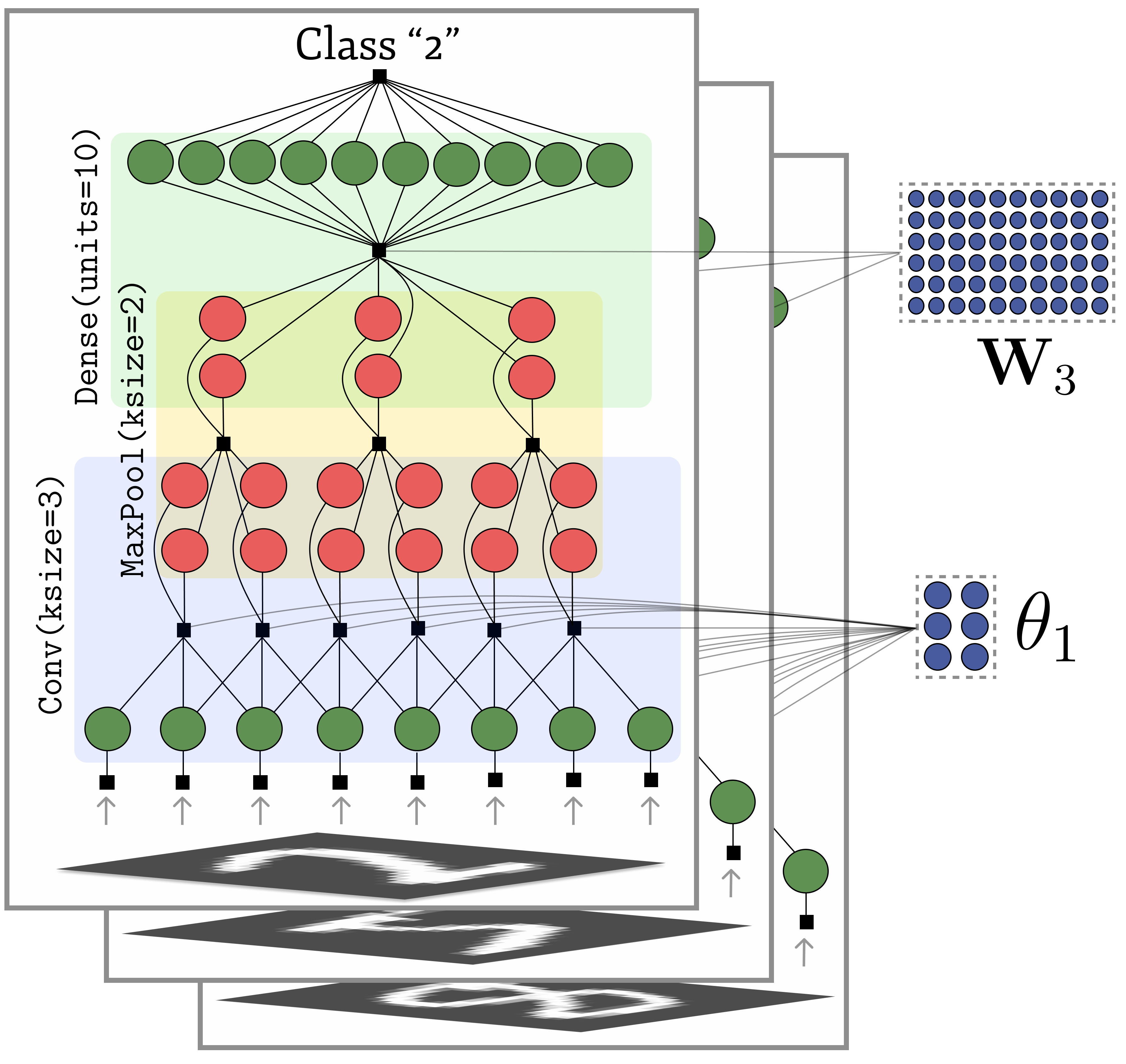
CNNs, which have been successfully applied across a range of computer vision tasks, have a sparse connectivity structure which suggests efficient factor analogues. In our convolutional layers, a factor at spatial location $(a,b)$ connects to i) the $K_{l}\times K_{l}$ patch of the input within its receptive field, $\mathbf{X}_{l-1}^{(a,b)}\in\mathbb{R}^{K_{l}\times K_{l}\times C_{l-1}}$, ii) the corresponding activation variable for an output channel $c$, $\mathbf{x}_{l}^{(a,b,c)}\in\mathbb{R}^{C_{l}}$ and iii) the parameters: filters $\mathbf{\theta}_{l}^{(c)}\in\mathbb{R}^{K_{l}\times K_{l}\times C_{l-1}}$ and bias $b_{l}^{(c)}$ for output channel $c$, which are shared across the layer. The energy can be written as:

$$E_{\mathrm{conv}}^{(a,b,c)} =\frac{\left(x_{l}^{(a,b,c)}-r\left(\mathbf{X}_{l-1}^{(a,b)},\mathbf{\theta}_{l}^{(c)},b_{l}^{(c)}\right)\right)^{2}}{2\sigma_{l}^{2}}~{},$$ (11)

where:

$$r\left(\mathbf{A},\mathbf{B},k\right) :=g\left(\mathrm{vec}\left(A\right)\cdot\mathrm{vec}\left(B\right)+k\right)~{}.$$ (12)

$g(\cdot)$ is an elementwise nonlinear activation function, and we have removed the functional dependence of $E_{\mathrm{conv}}^{(a,b,c)}$ on the connected variables for brevity. The total energy of the layer is found by summing $E_{\mathrm{conv}}^{(a,b,c)}$ over spatial locations $(a,b)$ and output channels $c$.

We can similarly define a transposed convolution layer. In this case, each filter is weighted by the output variable of its corresponding channel, and the weighted sum reconstructs the inputs. Note that for a stride smaller than the kernel size, each input will belong to multiple receptive fields and they are summed over to give its reconstruction. For example, for a stride of one, and neglecting edge effects we have:

$$E_{\mathrm{convT}}^{(a,b,c)} =\frac{\left(x_{l-1}^{(a,b,c)}-r\left(\mathbf{X}_{l}^{(a-i,b-j)},\mathbf{\theta}_{l}^{(i,j,c)},b_{l}^{(c)}\right)\right)^{2}}{2\sigma_{l}^{2}}~{}.$$ (13)

Note that in this case the parameters have dimensions $\mathbf{\theta}_{l}^{(c)}\in\mathbb{R}^{K_{l}\times K_{l}\times C_{l}}$ and $b_{l}^{(c)}\in\mathbb{R}^{C_{l-1}}$.

In addition to convolutions, we introduce factors akin to other common CNN layers. For example, we use max-pooling factors to reduce the spatial extent of the representation. For an input patch from channel $c$, $\mathbf{X}_{l-1}^{(a,b,c)}\in\mathbb{R}^{K\times K}$, centred at $(a,b)$, the connected pooling factor has energy:

$$E_{\mathrm{maxpool}}^{(a,b,c)} =\frac{1}{2\sigma_{l}^{2}}\left(\max\left(\mathbf{X}_{l-1}^{(a,b,c)}\right)-x_{l}^{(a,b,c)}\right)^{2}~{}.$$ (14)

For image classification, we use a dense projection head which translates the activation variables for the preceding layer $\mathbf{X}_{L-1}\in\mathbb{R}^{H_{L-1}\times W_{L-1}\times C_{L-1}}$ to a vector $\mathbf{x}_{L}\in\mathbb{R}^{C_{L}}$, where $C_{L}$ is the number of image classes. The dense factor energy is:

$$E_{\mathrm{dense}} =\frac{\left\lVert\mathbf{x}_{L}-\left(\mathbf{W}_{L}^{\top}\mathrm{vec}\left(\mathbf{X}_{L-1}\right)+\mathbf{d}_{L}\right)\right\rVert_{2}^{2}}{2\sigma_{L}^{2}}~{}.$$ (15)

Last, class supervision may then be incorporated by treating last layer activations $\mathbf{x}_{L}$ as logits and connecting them to a observation factor with energy:

$$E_{\mathrm{softmax}} =\frac{\left\lVert\mathrm{softmax}\left(\mathbf{x}_{L}\right)-\mathbbm{1}_{y}\right\rVert_{2}^{2}}{\sigma_{\mathrm{softmax}}^{2}}~{},$$ (16)

where $\mathbbm{1}_{y}$ is a one-hot encoding of the observed class $y$.

The “layer” abstractions defined above can be composed to produce deep models with similar design freedom to NNs. Similarly, our models may be overparameterised by introducing large numbers of learnable weights and we believe that the inclusion of non-linear activation functions $\mathbf{g}(\cdot)$ in our factor graph can aid representation learning as in DL. In particular, we note that for non-linear factors the Jacobian is a function of the variable values $\mathbf{J}_{j}=\mathbf{J}_{j}\left(\mathbf{x}_{\phi_{j},0}\right)$, which will cause the strength of the factors (9) to vary depending on the input data. We expect this to produce a similar “soft switching” of connections as observed in non-linear NNs. Note that the set of layers described here are non-exhaustive, and the translation of other neural architectures into factor graphs may be a worthwhile future direction.

3.2 Continual Learning

We now describe how we can do continual learning of our model parameters with Bayesian filtering. For generality, we use $\mathbf{\Psi}=\{\mathbf{\psi}_{l}\}_{l=1}^{L}$ to denote the set of all parameters where $\mathbf{\psi}_{l}$ is the vector of parameters for layer $l$. After initialising parameter priors $p_{t=1}\left(\mathbf{\psi}_{l,i}\right)\leftarrow\mathcal{N}\left(0,\sigma\right)$ we perform the following for each task $t$ in the sequence of datasets $[\mathbf{z}_{1},\ldots,\mathbf{z}_{T}]$:

1. construct a new graph with task dataset $\mathbf{z}_{t}$,

2. connect a unary prior factor to each parameter variable, equal to the marginal posterior estimate from the previous task $p_{t}\left(\mathbf{\psi}_{l,i}\right)\leftarrow p\left(\mathbf{\psi}_{l,i}|\mathbf{z}_{1:t-1}\right)$,

3. Run GBP training to get an estimate of the updated posterior $p(\mathbf{\Psi})=\prod_{l}\prod_{i=1}^{|\mathbf{\psi}_{l}|}p\left(\mathbf{\psi}_{l,i}|\mathbf{z}_{1:t}\right)$.

This method is equivalent to doing message passing in the combined graphical model for all tasks, but where messages between tasks are only passed forward in $t$. The advantage however, is that datapoints can be discarded after processing, and the combined graphical model for all tasks does not have to be stored in memory. As such, we also use this routine for memory-efficient training by dividing the dataset into minibatches and treating each minibatch as a task.

3.3 Efficient Gaussian Belief Propagation

3.3.1 Factor to Variable Message Optimisation

Efficient inference is a prerequisite to our models being applicable in practice. However, the inversion of a $\left(V_{j}-1\right)\times\left(V_{j}-1\right)$ matrix to compute $\Sigma_{\setminus i,\setminus i}^{\left(\phi_{j}+m\right)}$ in (8) is $O\left((V_{j}-1)^{3}\right)$ complexity, bottlenecking GBP. To alleviate this, we exploit the structure of matrix being inverted. In particular, i) for factors with observation dimension $M=\dim\left(\mathbf{y}\right)<V_{j}$, the precision $\Lambda^{(\phi_{j})}$ (9) is low-rank, and ii) for graphs with scalar variable nodes, $\mathbf{D}$ is diagonal. Thus their sum may be efficiently inverted via the Woodbury identity (woodbury1950inverting). Further savings come from reusing intermediates when computing messages to multiple variables (9). These optimisations change the complexity of updating messages from a factor to all $V$ variables, from $O(V\left(V-1\right)^{3})$ to $O\left(VM^{3}\right)$. Space complexity is changed from $O(V^{2})$ to $O(VM+M^{2})$. Both are significant savings when $M<<V$. See App. A for details.

3.3.2 Implementation

Our factor graphs have regular, repeated structure making our GBP amenable to GPU parallelisation. We implement our method in TensorFlow (Tensorflow:MISC2015) to make use of GPU support and efficient linear algebra operations. For a given batch, we initialise the graph and update the messages by sweeping forward and backward through the layers: first the layer nearest the input observations, then progressively deeper to the deepest layer and back again. We repeat these sweeps for a specified number of iterations. When updating the messages within each layer, we parallelise all factor to variable messages, and likewise for the variable to factor updates of each variable type (inputs, outputs, parameters as applicable). This message schedule is likely suboptimal, but we leave further exploration for future work. We find that applying damping (murphy2013loopy) and dropout to the factor to variable message updates is sufficient for stable GBP.

For supervised learning experiments, the output observation factors are only included at training time. At test time, we predict by running GBP in the test graph and taking the last layer variables as regression predictions or logits. As our factor graph is a joint model of both inputs and labels we could, in theory, continue to learn from the input distribution at test time. In practice we find performance is slightly better when we fix the learnt parameters, and run GBP on the input, output and activations.

4 Results

We demonstrate the benefits of our approach with three experiments: some small regression tasks, sequential video denoising and continual learning for image classification. The corresponding code is made available.

(a) Architecture

(b) XOR, $p(y=1|\mathbf{x}_{1},\mathbf{W}_{1},\mathbf{W}_{2})$

(c) Nonlinear regression

Figure 2: GBP learning in MLP-like factor graphs (2(a)) can solve nonlinear regression and classification tasks.

4.1 Toy Experiments

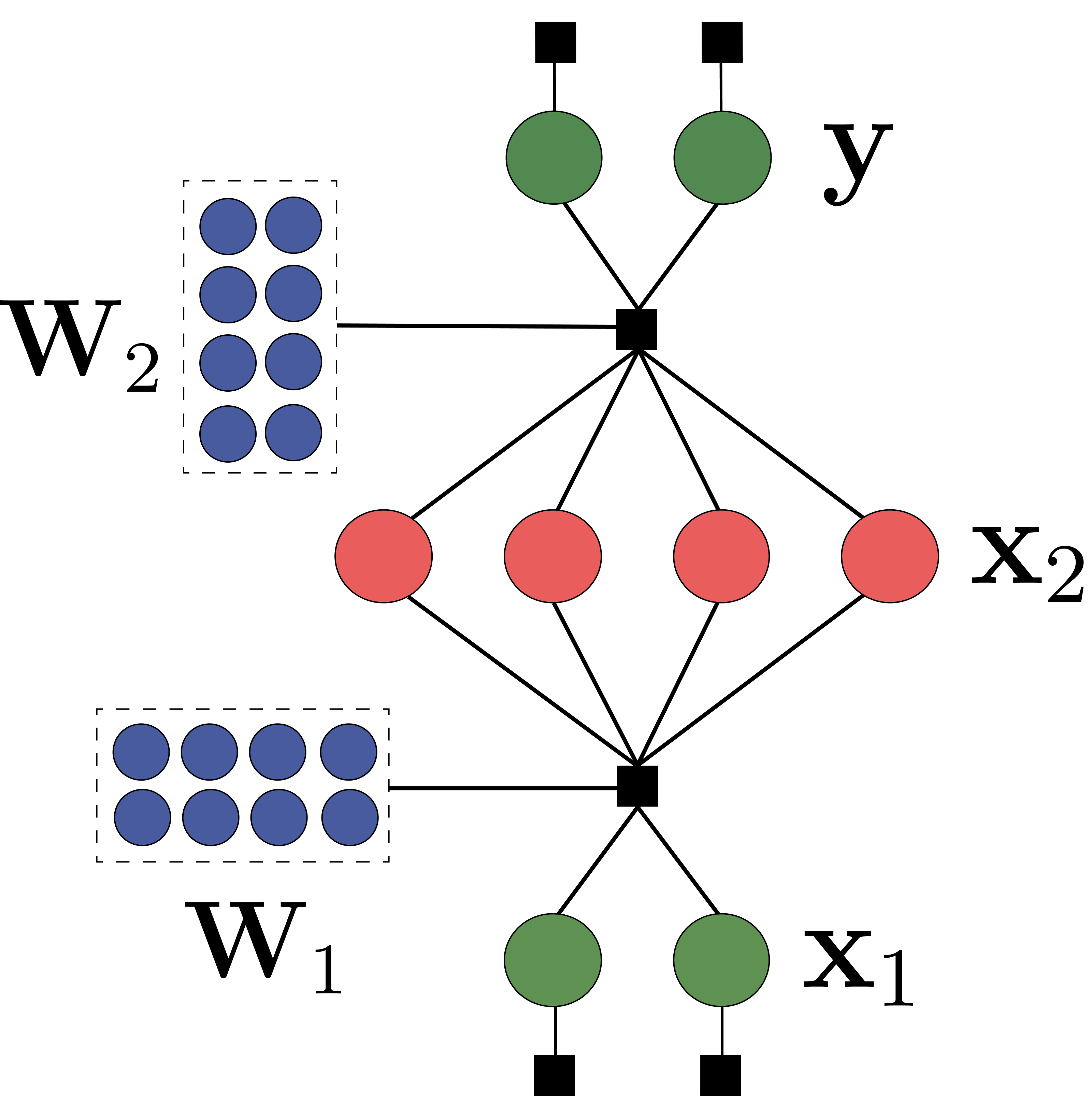
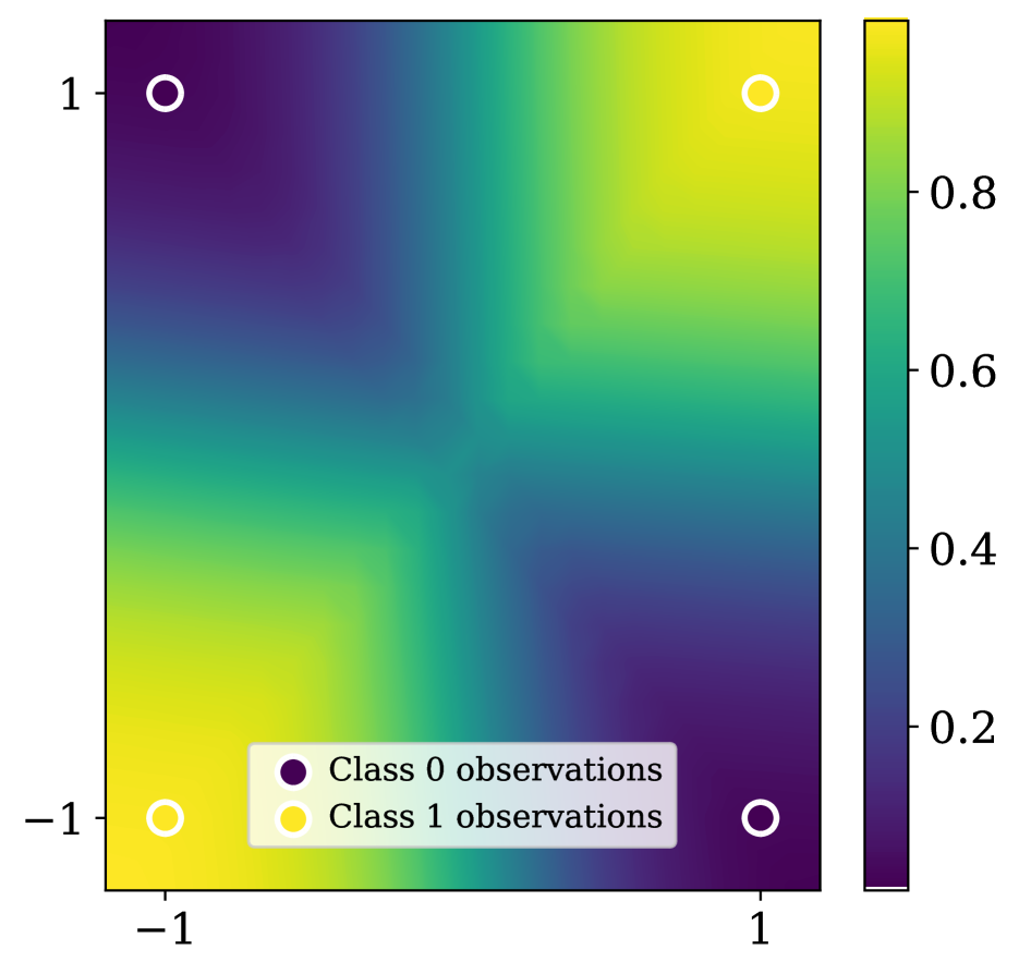
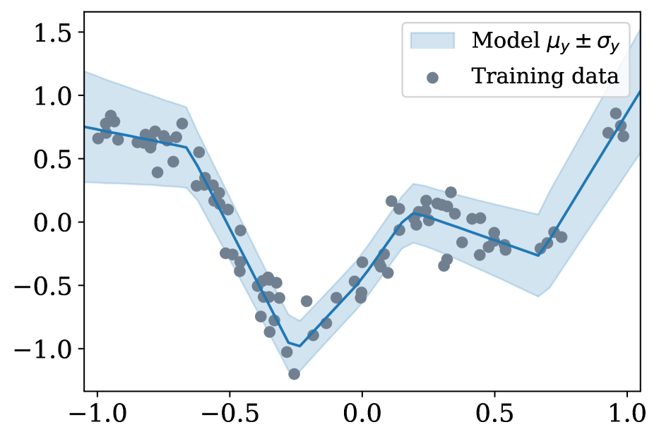
We start by verifying that our model can solve tasks requiring nonlinear modelling. To this end, we run GBP learning with single hidden layer, MLP-like factor graphs (Fig. 2(a)) in two settings. The first is “Exclusive-OR”, which is a well-known minimal test for nonlinear modelling (Fig. 2(b)). The second is a nonlinear regression problem (Fig. 2(c)) with $90$ training points. In both cases, we employ a Leaky ReLU activation in the first dense layer. Full details are provided in App. B. It is clear that GBP learning can solve both tasks, confirming that the linearisation method described in Section 2.3 is sufficient to capture nonlinear dependencies.

4.2 Video Denoising

Figure 3: Video denoising results. Factor graphs with learnable components outperform a hand-specified pairwise smoother with robust factors, and continual learning of the parameters throughout the video further improves performance over per-frame learning. Shaded regions cover $\pm 2$ standard errors (SEs) over $10$ seeds.

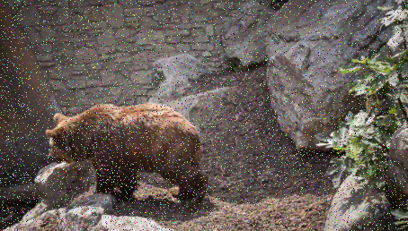
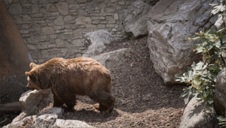
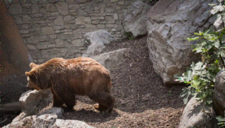
We now ask whether the learnable components in our model can improve performance over a hand-designed solver. We apply our method to the task of denoising the “bear” video from the DAVIS dataset (perazzi2016benchmark), downsampled to $258\times 454$ with bilinear interpolation. We randomly select $10\%$ of the pixels in each frame of the video, and replace their intensities with noise independently sampled from $U(0,1)$. Performance is assessed by how well the denoised image matches the ground truth according to the peak signal-to-noise ratio (PSNR).

We run GBP learning with two models: i) a single transposed convolution layer with four filters, and ii) a five layer model comprising stacked transposed convolution and upsampling layers (see App. C). Both the pixel observation and reconstruction factors have robust energies (see Section 5 of Davison:Ortiz:ARXIV2019 for details) to enable the pixel variables to “switch” between being explained by the noisy observation or by the reconstruction model. As a baseline, we compare to a classical pairwise smoothing model in which neighbouring pixels are encouraged to have similar intensities through smoothness factors shared between adjacent pixels (see e.g ortiz2021visual). Robust energies for these factors aid the preservation of edges present in the original image. The baseline also includes robust energies for pixel observation factors, as in our model.

In both pairwise smoother and GBP learning, we do inference with GBP. Note that in our models, this is jointly estimating the true pixel intensities and the model parameters. We emphasise that our model learns image structure from the noisy images only and without supervision. It is incentivised to do so by the reconstruction factors in noiseless regions. We evaluate two routines for training the parameters: i) learn them from scratch on each frame and ii) do filtering on the parameters over the sequence of frames, with the approach described in Section 3.2. The hyperparameters for all models were tuned using the first five frames of the video. Further details of the final models can be found in App. C. Denoising the entire $82$-frame video with the single layer model took $\sim 8$mins on a NVIDIA RTX 3090 GPU, and the five layer model took $\sim 27$mins. Pairwise smoothing took $\sim 2$mins.

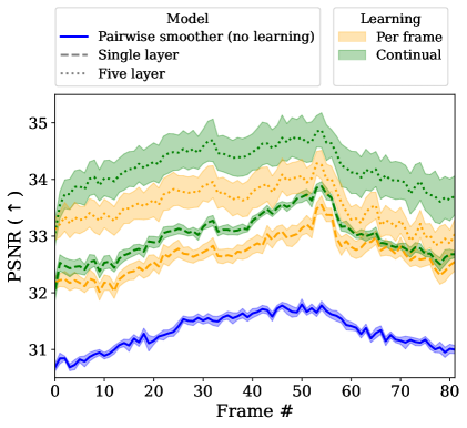
The PSNR results are presented in Fig. 3 (and examples of denoised frames in Fig. D1). The models with learnable parameters (orange and green) significantly outperform the classical baseline (blue). We attribute this to the learned models being able to capture image structure, which enables more high-frequency features to be retained while removing the corruption. All methods exhibit a similar relative evolution of PSNR over the course of the video, slowing rising until the fiftieth frame and then falling again. We conjecture that this is due to variations in the content of the images, with some frames being easier to denoise than others.

There is clear benefit of depth, with significantly higher PSNR scores for the five layer model (orange/green dotted) compared to the single layer model (orange/green dash). Despite the single layer model having only four filters, we find that it overfits during continual learning. To counteract this, we set the prior for each frame to be an interpolation between the previous posterior and the original prior (plotted; see App. C). In contrast, the deeper model does not require additional regularisation when learning continually. These results imply i) deep factor graphs can have better inductive biases, ii) GBP learning is effective in finding aligned multi-layer representations with only local message updates.

In general we see that continual learning leads to an improvement over learning per-frame, suggesting that we can effectively fuse what has been learnt in previous frames and use it to better denoise the current frame.

4.3 Image Classification

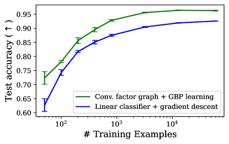
Next, we assess our method in a supervised learning context, evaluating it on MNIST. We train a convolutional factor graph with architecture similar to Fig. 1: a convolutional layer (with energy as per (11)), followed by a max-pool (14), dense layer (15) and (at train time) a class observation factor (16) on the output logit variables. Training is minibatched via the Bayesian filtering approach described in Section 3.2, so the model only sees each datapoint once after which it can be discarded. Full details of the model are in App. E.1. To gauge sample efficiency, we train on subsets of varying sizes, as well as the full training set. We compare against a linear classifier baseline which predicts logits via a dense projection of the image. This baseline is trained with gradient descent. Further details of the baseline are included in App. E.2. Both models were tuned on validation sets generated by randomly subsampling $15\%$ of the training set.

We find the GBP Learning in the deep model achieves a test accuracy of $96.3\%$ when trained on the full training set (Fig. 4), significantly higher than the linear classifier ($92.6\%$). This implies that our approach can learn useful features and capture nonlinear relationships. In addition, our method shows better sample efficiency, beating the baseline for every training set size, despite only seeing each datapoint once. In contrast, the linear classifier is trained for multiple epochs. We also trained our model in a layer-wise asynchronous manner by uniformly sampling a layer whose messages to update at each step. Such an approach yields a final accuracy of $96.35\pm 0.03\%$ ($\pm 1$SE over $3$ seeds), indistinguishable from $96.4\pm 0.2\%$ achieved by the same model trained with synchronous forward/backward sweeps (details in App. E.3). This result implies that GBP Learning can work well when the model is distributed over multiple processors, without the need for global synchronisation. We find the GBP Learning in the deep model achieves a test accuracy of $96.3\%$ when trained on the full training set (Fig. 4), significantly higher than the linear classifier ($92.6\%$). This implies that our approach can learn useful features and capture nonlinear relationships. In addition, our method shows better sample efficiency, beating the baseline for every training set size, despite only seeing each datapoint once. In contrast, the linear classifier is trained for multiple epochs. We also trained our model in a layer-wise asynchronous manner by uniformly sampling a layer whose messages to update at each step. Such an approach yields a final accuracy of $96.35\pm 0.03\%$ ($\pm 1$SE over $3$ seeds), indistinguishable from $96.4\pm 0.2\%$ achieved by the same model trained with synchronous forward/backward sweeps (details in App. E.3).

Full dataset training with GBP Learning takes around $3$ hours on NVIDIA RTX 3090 GPU. While this is considerably slower than the few minutes it took to train the linear classifier on CPU (and would take to train a small NN), we note that the software to train such models has benefited from decades of optimisation, as have well-established hardware platforms like GPUs. In contrast, our current GBP Learning implementation runs on a hardware and software stack optimised for a different set of models. We believe orders of magnitude efficiency gains could be made by running GBP Learning on a more tailored setup including modern processors with significant on-chip memory. See Section 6 for further discussion.

Figure 4: MNIST results. A deep factor graph trained with GBP learning outperforms a linear model trained with gradient descent, over a pareto front of training set sizes. Error bars cover $\pm 2$ SEs over $5$ random seeds.

5 Related Work

Our models can be viewed as probabilistic energy-based models (EBMs lecun2006tutorial; du2019implicit) whose energy functions are the sum of the quadratic energies for all factors in the graph. The benefit of using a Gaussian factor graph is a model which normalises in closed form without resorting to expensive and tricky-to-tune MCMC sampling. While the quadratic energy may seem constraining, we add capacity with the introduction of non-linear factors and overparameterisation. For most EBMs, parameters are viewed as attributes of the factors, where we include them as variables in our graph. As a result, learning and inference are a single combined procedure in our approach, but two distinct stages for other EBMs.

Of the EBM family, restricted Boltzmann machines (RBMs smolensky1986information) are of particular relevance. Their factor graph resembles a single layer, fully connected version of our model, however RBMs are models over discrete variables which are unable capture the statistics of continuous natural images. While exponential family generalisations exist, such as Gaussian-Bernoulli RBMs (welling2004exponential), scaling RBMs to multiple layers remains a challenging problem. To our knowledge there are no working examples of training stacked RBMs jointly, instead they are trained greedily with each layer learning to reconstruct the fixed activations of the previous layer after it has converged (hinton2006fast; hinton2006reducing). As an artefact of this, later layers use capacity in learning the artificial correlations introduced by the previous layers rather than residual correlations present in the data. Global alignment is then found by fine tuning with either backprop (hinton2006reducing) or wake-sleep (hinton2006fast). We have found BP training to work in multiple layer factor graphs without issue.

Our approach also relates to Bayesian DL (neal2012bayesian) in that we seek to infer a distribution over parameters of a deep network. However, common methods to train Bayesian NNs (BNNs) are based on e.g. optimising a variational objective (blundell2015weight; gal2016dropout), the Laplace approximation (mackay1992practical; ritter2018scalable), Hamiltonian Monte Carlo (neal2012bayesian), Langevin-MCMC (zhang2019cyclical). Each of these methods comes with their own benefits and drawbacks but we note two features of our method which distinguish it from existing work in this field. The first is a unified procedure of training and prediction, which are two separate stages in existing methods. The second is our activations are random variables, allowing us to model (and resolve) disagreement between bottom-up and top-down signals.

Much work has focused on augmenting BP with DL (nachmani2016learning; satorras2021neural; yoon2019inference; lazaro2021query). In contrast, our method does DL within a BP framework. george2017generative also propose a hybrid vision system in which visual features and graph structure are learnt in a separate process to the discrete BP routine used to parse scenes (given features and graph). lazaro2016hierarchical is more similar to ours in that parameters are treated as variables in the graphical model and updated with BP. However, their factor graph comprises only binary variables, making it ill-suited to natural images. In addition, max-product BP is used which only finds a MAP solution, and not a full posterior estimate. This precludes the ability to learn incrementally via Bayesian filtering.

6 Conclusions

We have introduced GBP Learning, a method for learning in Gaussian factor graphs. Parameters are included as variables in the graph and learnt using the same BP inference procedure used to estimate all other latent variables. Inter-layer factors encourage representations to be locally consistent, and multiple layers can be stacked in order to learn richer abstractions. Experimentally, we have seen a shallow, learnable model can outperform a hand-crafted method on a video denoising task, with further performance gains coming from stacking multiple layers. We have also applied GBP Learning to train a convolutional factor graph on MNIST. The results show it outperforms a linear classifier both in terms of sample efficiency and peak accuracy, despite only seeing each datapoint once. Both sets of experiments demonstrate the efficacy of our continual learning approach.

While we find these initial results encouraging, we highlight scaling up GBP Learning to bigger, more complex models and datasets as an exciting future direction. Our current implementation is built on software and run on hardware heavily optimised for deep learning. Scaling up GBP Learning requires engineering a bespoke hardware/software system, which can better leverage the distributed nature of GBP inference. In particular, we believe processors with memory local to the compute cores (Graphcore; cerebras) to be a promising platform for efficient BP. On such processors, different sections of the factor graphs could be mapped to different cores. Local message updates, between factors and variables on the same core, would be cheap and could be updated at high frequency, with occasional inter-core communication to ensure alignment between different parts of the model. Low-level GBP primitives, written in e.g. Poplar, could be used to ensure the message updates make efficient use of high-bandwidth, local memory. A similar system was applied to solving bundle adjustment problems with GBP, and was found to be around $35\times$ faster on IPU (Graphcore) than a commonly used CPU-based solver.

xmain_preprint.bbl

 

Supplementary Material for Learning in Deep Factor Graphs with Gaussian Belief Propagation

 

Appendix A Factor to Variable Message Update Optimisation

We aim to reduce the complexity of message update computations (8). Naiv̈e inversion of the sum of factor and message precisions $\Sigma_{\setminus i,\setminus i}^{\left(\phi_{j}+m\right)}=\left(\Lambda^{\left(\phi_{j}\right)}_{\setminus i,\setminus i}+\left(\mathbf{D}_{\phi_{j}}\right)_{\setminus i,\setminus i}\right)^{-1}$ has complexity $O\left(\left(V_{j}-1\right)^{3}\right)$. This can be reduced to $O\left(\left(V-1\right)M^{2}+M^{3}\right)$ ($M:=\dim\mathbf{y}$) by substituting $\Lambda^{(\phi_{j})}$ for the linearised factor precision (9) and applying the Woodbury identity (woodbury1950inverting):

$$\mathbf{S}_{\setminus i}=\mathbf{D}_{\setminus i,\setminus i}^{-1}-\mathbf{D}_{\setminus i,\setminus i}^{-1}\left(\mathbf{J}_{:,\setminus i}\right)^{{}^{\top}}\left(\Lambda_{\mathbf{y}}^{-1}-\mathbf{J}_{:,\setminus i}\mathbf{D}_{\setminus i,\setminus i}^{-1}\left(\mathbf{J}_{:,\setminus i}\right)^{{}^{\top}}\right)^{-1}\mathbf{J}_{:,\setminus i}\mathbf{D}_{\setminus i,\setminus i}^{-1}~{},$$ (17)

where we have dropped subscripts and superscripts relating to $\phi_{j}$ for brevity.

Further efficiencies come from substituting (17) back into the factor to variable message update (8),

$$\Lambda_{{\phi\rightarrow x_{i}}} \leftarrow\Lambda_{i,i}-\Lambda_{i,\setminus i}\left(\mathbf{D}_{\setminus i,\setminus i}^{-1}-\mathbf{D}_{\setminus i,\setminus i}^{-1}\left(\mathbf{J}_{:,\setminus i}\right)^{{}^{\top}}\left(\Lambda_{\mathbf{y}}^{-1}-\mathbf{J}_{:,\setminus i}\mathbf{D}_{\setminus i,\setminus i}^{-1}\left(\mathbf{J}_{:,\setminus i}\right)^{{}^{\top}}\right)^{-1}\mathbf{J}_{:,\setminus i}\mathbf{D}_{\setminus i,\setminus i}^{-1}\right)\Lambda_{\setminus i,i}$$ (18)

$$\eta_{{\phi\rightarrow x_{i}}} \leftarrow\eta_{i}-\Lambda_{i,\setminus i}\left(\mathbf{D}_{\setminus i,\setminus i}^{-1}-\mathbf{D}_{\setminus i,\setminus i}^{-1}\left(\mathbf{J}_{:,\setminus i}\right)^{{}^{\top}}\left(\Lambda_{\mathbf{y}}^{-1}-\mathbf{J}_{:,\setminus i}\mathbf{D}_{\setminus i,\setminus i}^{-1}\left(\mathbf{J}_{:,\setminus i}\right)^{{}^{\top}}\right)^{-1}\mathbf{J}_{:,\setminus i}\mathbf{D}_{\setminus i,\setminus i}^{-1}\right)\eta_{\setminus i}^{(\phi+m)}~{},$$ (19)

and noting that $$\Lambda_{i,\setminus i}=\left(\mathbf{J}_{:,i}\right)^{{}^{\top}}\Lambda_{\mathbf{y}}\mathbf{J}_{:,\setminus i}$$. We can then write:

$$\Lambda_{{\phi\rightarrow x_{i}}} \leftarrow\Lambda_{i,i}-\left(\mathbf{J}_{:,i}\right)^{{}^{\top}}\Lambda_{\mathbf{y}}\mathbf{J}_{:,\setminus i}\left(\mathbf{D}_{\setminus i,\setminus i}^{-1}-\mathbf{D}_{\setminus i,\setminus i}^{-1}\left(\mathbf{J}_{:,\setminus i}\right)^{{}^{\top}}\left(\Lambda_{\mathbf{y}}^{-1}-\mathbf{J}_{:,\setminus i}\mathbf{D}_{\setminus i,\setminus i}^{-1}\left(\mathbf{J}_{:,\setminus i}\right)^{{}^{\top}}\right)^{-1}\mathbf{J}_{:,\setminus i}\mathbf{D}_{\setminus i,\setminus i}^{-1}\right)\left(\mathbf{J}_{:,\setminus i}\right)^{{}^{\top}}\Lambda_{\mathbf{y}}\mathbf{J}_{:,i}$$ (20)

$$\eta_{{\phi\rightarrow x_{i}}} \leftarrow\eta_{i}-\left(\mathbf{J}_{:,i}\right)^{{}^{\top}}\Lambda_{\mathbf{y}}\mathbf{J}_{:,\setminus i}\left(\mathbf{D}_{\setminus i,\setminus i}^{-1}-\mathbf{D}_{\setminus i,\setminus i}^{-1}\left(\mathbf{J}_{:,\setminus i}\right)^{{}^{\top}}\left(\Lambda_{\mathbf{y}}^{-1}-\mathbf{J}_{:,\setminus i}\mathbf{D}_{\setminus i,\setminus i}^{-1}\left(\mathbf{J}_{:,\setminus i}\right)^{{}^{\top}}\right)^{-1}\mathbf{J}_{:,\setminus i}\mathbf{D}_{\setminus i,\setminus i}^{-1}\right)\eta_{\setminus i}^{(\phi+m)}~{}.$$ (21)

Right-multiplying the $$\mathbf{J}_{:,\setminus i} (\mathbf{J}_{:,\setminus i})^{{}^{\top}}$$ before the parentheses, and left multiplying the after gives

$$\Lambda_{{\phi\rightarrow x_{i}}} \leftarrow\Lambda_{i,i}-\left(\mathbf{J}_{:,i}\right)^{{}^{\top}}\Lambda_{\mathbf{y}}\left(\mathbf{U}_{i}-\mathbf{U}_{i}\left(\Lambda_{\mathbf{y}}^{-1}-\mathbf{U}_{i}\right)^{-1}\mathbf{U}_{i}\right)\Lambda_{\mathbf{y}}\mathbf{J}_{:,i}~{},$$ (22)

where we have defined $$\mathbf{U}_{i}:=\mathbf{J}_{:,\setminus i}\mathbf{D}_{\setminus i,\setminus i}^{-1}\left(\mathbf{J}_{:,\setminus i}\right)^{{}^{\top}} \eta_{\setminus i}^{(\phi+m)}$$. For the information update, we instead right-multiply

$$\eta_{{\phi\rightarrow x_{i}}} \leftarrow\eta_{i}-\left(\mathbf{J}_{:,i}\right)^{{}^{\top}}\Lambda_{\mathbf{y}}\left(\mathbf{T}_{i}-\mathbf{U}_{i}\left(\Lambda_{\mathbf{y}}^{-1}-\mathbf{U}_{i}\right)^{-1}\mathbf{T}_{i}\right)~{}.$$ (23)

where $\mathbf{T}_{i}:=\mathbf{J}_{:,\setminus i}\mathbf{D}_{\setminus i,\setminus i}^{-1}\eta_{\setminus i}^{(\phi+m)}$. Given $\mathbf{U}_{i}$ and $\mathbf{T}_{i}$, both message updates are $O\left(M^{3}\right)$, i.e. independent of $V$. However direct computation of $\mathbf{U}_{i}$ or $\mathbf{T}_{i}$ has complexity $O\left((V-1)M^{2}\right)$ for each outgoing variable $i$ ($\mathbf{D}^{-1}$ is diagonal), so the overall complexity is quadratic in $V$. We achieve linear complexity by exploiting $\mathbf{U}_{i}=\mathbf{J}\mathbf{D}^{-1}\mathbf{J}^{{}^{\top}}-\mathbf{J}_{:,i}\mathbf{D}_{i,i}^{-1}\left(\mathbf{J}_{:,i}\right)^{{}^{\top}}$ where $\mathbf{J}\mathbf{D}^{-1}\mathbf{J}^{{}^{\top}}$ can be computed once for all connected variables. Similarly, we use $\mathbf{T}_{i}=\mathbf{J}\mathbf{D}^{-1}\eta^{(\phi+m)}-\mathbf{J}_{:,i}\mathbf{D}_{i,i}^{-1}\eta_{i}^{(\phi+m)}$ for the information update. This reduces the complexity for updating all outgoing messages from a factor from $O\left(V\left(\left(V-1\right)M^{2}+M^{3}\right)\right)$ to $O\left(VM^{3}\right)$. In addition, these optimisations require memory $O\left(VM+M^{2}\right)$ which, in most cases, is a saving relative to $O\left(V^{2}\right)$ needed to store the full factor precision.

Appendix B Toy Experiment Details

B.1 XOR

We use the MLP-inspired factor graph architecture illustrated in Fig. 2(a), with $8$ units in the hidden layer and a Leaky ReLU activation in the first-layer dense factor. The full model is described in Table 1.

We run GBP in the training graph (with $4$ input/output observations) for $600$ iterations. We then fix the parameters, remove the softmax class observation layer and run GBP for $300$ iterations on a grid of $20\times 20$ test input points. The last layer activation variables are then treated as the logits for class predictions. At both train and test time, we use a damping factor of $0.8$ and a dropout of $0.5$ in the factor to variable message updates from the dense factors.

Layer #	$1$	$2$	$3$
Layer type	Dense	Dense	Softmax
Input dim.	$2$	$8$	$2$
Output dim.	$8$	$2$	$2$
Inc. bias	✓	✓	N/A
Weight prior $\sigma$	$3.0$	$3.0$	N/A
Activation prior $\sigma$	$5.0$	$2.0$	N/A
Input obs. $\sigma$	$0.02$	N/A	N/A
Class obs. $\sigma$	N/A	N/A	$0.1$
Dense recon. $\sigma$	$0.1$	$0.1$	N/A
Activation function $g(\cdot)$	Leaky ReLU	Linear	N/A

Table 1: The MLP-like factor graph used for the XOR experiment.

B.2 Regression

To generate the 1D regression data, we sample the $90$ input points uniformly in the interval $(-1.0,1.0)$. For each input point $x_{i}$, the output $y_{i}$ is generated according to

$$z_{i} =5\cdot\sin\left(6.7\cdot x_{i}\right)+\left(10\cdot x\right)^{2}*0.15+\epsilon_{i}~{},$$ (24)

$$y_{i} =\frac{z_{i}-\mathrm{mean}\left(z\right)}{2\cdot\mathrm{std}\left(z\right)}$$ (25)

where

$$\epsilon_{i} \sim\mathcal{N}(0.,1.5)$$ (26)

and $\mathrm{mean}\left(\cdot\right)$, $\mathrm{std}\left(\cdot\right)$ are empirical estimates over the $90$ training points.

To fit the data, we use a similar MLP-inspired factor graph architecture to that illustrated in Fig. 2(a). However, this architecture has only $1$ input variable and $1$ output variable. We use $16$ units in the hidden layer and a Leaky ReLU activation in the first-layer dense factor. The full model is described in Table 2.

We run GBP in the training graph (with $90$ input/output observations) for $2000$ iterations. We then fix the parameters, remove the output observation layer and run GBP for $1000$ iterations on $225$ uniformly spaced test input points. The last layer activation variables are then treated as the predictions for these query points. At both train and test time we use a damping factor of $0.8$ and a dropout of $0.6$ in the factor to variable message updates from the dense factors.

Layer #	$1$	$2$	$3$
Layer type	Dense	Dense	Output observation
Input dim.	$1$	$16$	$1$
Output dim.	$16$	$1$	$1$
Inc. bias	✓	✓	N/A
Weight prior $\sigma$	$7.0$	$7.0$	N/A
Activation prior $\sigma$	$5.0$	$1.0$	N/A
Input obs. $\sigma$	$0.02$	N/A	N/A
Output obs. $\sigma$	N/A	N/A	$0.03$
Dense recon. $\sigma$	$7\times 10^{-3}$	$7\times 10^{-3}$	N/A
Activation function $g(\cdot)$	Leaky ReLU	Linear	N/A

Table 2: The MLP-like factor graph used for the regression experiment.

Appendix C Video Denoising Experiment Details

C.1 Single Layer Convolutional Factor Graph

We use the transposed convolution model described in Table C1 for both per-frame and continual learning experiments. We run for $300$ GBP iterations on each frame with damping factor of $0.8$ and dropout factor of $0.6$ applied to the factor to variable messages. We used robust factor energies similar to the Tukey loss (Tukey:1960): quadratic within a Mahalanobis distance of $N_{\mathrm{rob}}$ from the mean, and flat outside.

Layer #	1
Layer type	Transposed Conv.
Number of filters	4
Inc. bias	✓
Kernel size	$3\times 3$
Conv. recon. $\sigma$	0.1
Recon $N_{\mathrm{rob}}$	1.4
Weight prior $\sigma$	0.018
Activation prior $\sigma$	0.5
Pixel obs. $\sigma$	0.2
Pixel obs $N_{\mathrm{rob}}$	0.2
Activation function $g(\cdot)$	Linear

Table C1: The single layer convolutional factor graph model used for the video denoising experiments. $N_{\mathrm{rob}}$ is the “robust threshold”: the Mahalanobis distance beyond which the factor energy is flat rather than quadratic.

C.1.1 Preventing overfitting in single-layer model

We find the single-layer convolutional model described above can overfit to the salt-and-pepper noise when the filters are learnt continually over the course of the video. We find that overfitting can be reduced by choosing the parameter prior at each frame to be an interpolation of the previous parameter posterior and the original parameter prior.

More concretely, for a parameter $\mathbf{\theta}_{l,i}$ with original prior (before the first frame) $\mathcal{N}(\mathbf{\theta}_{l,i};\mu_{\theta_{l}},\sigma_{\theta_{l}}^{2})$ and posterior from previous frames $\mathcal{N}(\mathbf{\theta}_{l,i};\mu_{l,i}^{(t-1)},(\sigma_{l,i}^{(t-1)})^{2})$ we set its prior for a frame $t$ to be

$$p_{t}(\mathbf{\theta}_{l,i}) \leftarrow\mathcal{N}\left(\mathbf{\theta}_{l,i};\mu_{l,i},\left(\sigma_{l,i}\right)^{2}\right)~{},$$ (27)

where

$$\mu_{l,i} =\alpha\cdot\mu_{\theta_{l}}+(1-\alpha)\cdot\mu_{l,i}^{(t-1)}$$ (28)

$$\sigma_{l,i} =\alpha\cdot\sigma_{\theta_{l}}+(1-\alpha)\cdot\sigma_{l,i}^{(t-1)}~{}.$$ (29)

We used $\alpha=0.5$ for the single-layer, continual learning video denoising experiment.

C.2 Five Layer Convolutional Factor Graph

We use the transpose convolution model described in Table C2 for both per-frame and continual learning experiments. We run for $500$ GBP iterations on each frame with damping factor of $0.8$ and dropout factor of $0.6$ applied to the factor to variable messages. We used robust factor energies similar to the Tukey loss (Tukey:1960): quadratic within a Mahalanobis distance of $N_{\mathrm{rob}}$ from the mean, and flat outside.

To increase the spatial extent of the activations, we use upsampling layers within which each output $x_{l}^{(a,b,c)}$ connects to a $K\times K$ patch of the input $\mathbf{X}_{l-1}^{(a,b,c)}$ via a factor with energy

$$E_{\mathrm{upsample}} =\frac{1}{2\sigma^{2}}\sum_{i,j=-\lfloor K/2\rfloor{}}^{\lfloor K/2\rfloor{}}\left(x_{l-1}^{(a+i,b+j,c)}-x_{l}^{(a,b,c)}\right)^{2}~{}.$$ (30)

Layer #	1	2	3	4	5
Layer type	Transposed Conv.	Upsample	Transposed Conv.	Upsample	Transposed Conv.
Number of filters	4	N/A	8	N/A	8
Inc. bias	✓	N/A	✓	N/A	✓
Kernel size	$3\times 3$	$2\times 2$	$3\times 3$	$2\times 2$	$3\times 3$
Conv. recon. $\sigma$	0.12	0.03	0.07	0.03	0.07
Recon $N_{\mathrm{rob}}$	2.5	N/A	N/A	N/A	N/A
Weight prior $\sigma$	0.15	N/A	0.3	N/A	0.3
Activation prior $\sigma$	0.5	N/A	0.5	N/A	0.5
Pixel obs. $\sigma$	0.2	N/A	N/A	N/A	N/A
Pixel obs $N_{\mathrm{rob}}$	0.2	N/A	N/A	N/A	N/A
Activation func. $g(\cdot)$	Linear	N/A	Leaky ReLU	N/A	Leaky ReLU

Table C2: The five-layer convolutional factor graph model used for the video denoising experiments. $N_{\mathrm{rob}}$ is the “robust threshold”: the Mahalanobis distance beyond which the factor energy is flat rather than quadratic.

C.3 Pairwise Factor Graph

The factor hyperparameters for the pairwise smoother baseline are given in Table C3. We denoise by running $200$ GBP iterations on each frame with damping factor of $0.7$ applied to the factor to variable messages. We used robust factor energies similar to the Tukey loss (Tukey:1960): quadratic with a Mahalanobis distance of $N_{\mathrm{rob}}$ from the mean, and flat outside.

Layer #	1
Layer type	Pairwise smoothing
Pixel obs. $\sigma$	0.2
Pixel obs $N_{\mathrm{rob}}$	0.14
Pairwise $\sigma$	1.3
Pairwise $N_{\mathrm{rob}}$	0.35

Table C3: The pairwise smoothing baseline model used for the video denoising experiments. $N_{\mathrm{rob}}$ is the “robust threshold”: the Mahalanobis distance beyond which the factor energy is flat rather than quadratic.

Appendix D Denoised Video Frame Example

(a) Clean image

(b) Corrupted image

(c) Per-frame learning, single layer, $\mathrm{PSNR}=32.6$

(d) Continual learning, single layer, $\mathrm{PSNR}=32.9$

(e) Per-frame learning, five layer, $\mathrm{PSNR}=33.4$

(f) Continual learning, five layer, $\mathrm{PSNR}=34.3$

(g) Pairwise smoothing, $\mathrm{PSNR}=31.1$

Figure D1: Frame 5 denoised by each method.

(a) Clean image

(b) Corrupted image

(c) Per-frame learning, single layer

(d) Continual learning, single layer

(e) Per-frame learning, five layer

(f) Continual learning, five layer

(g) Pairwise smoothing

Figure D2: A crop from frame 5. The learnt models are able to remove more noise while retaining more high-frequency signal.

Appendix E MNIST experiment details

E.1 Deep Gaussian Factor Graph

For the MNIST experiment we tuned the factor graph architecture and the other hyperparameters on a validation set of $9,000$ examples sampled uniformly from the training set. We then used the same tuned model for every training set size.

The final convolutional factor graph model is summarised in Table E1. To produce the results shown in Fig. 4, we train with continual learning, with a batchsize of $50$ and run $800$ GBP iterations on each batch. At test time, we fix the parameters and run GBP for $500$ iterations per test batch of $200$ examples. We apply a damping factor of $0.9$ and a dropout factor of $0.5$ to the factor to variable messages at both train and test time. Note that each iteration includes the updating of the messages in each layer, sweeping from image layer to classification head, and then sweeping back to image.

Layer #	1	2	3	4†
Layer type	Conv.	Max pool	Dense	Softmax
Num. filters	8	N/A	N/A	N/A
Kernel size	$5\times 5$	$2\times 2$	N/A	N/A
Dense num. inputs	N/A	N/A	1152	N/A
Dense num. outputs	N/A	N/A	10	N/A
Inc. bias	✓	N/A	✓	N/A
Weight prior $\sigma$	0.04	N/A	0.3	N/A
Activation prior $\sigma$	1.0	1.0	2.0	N/A
Pixel obs. $\sigma$	0.03	N/A	N/A	N/A
Recon. $\sigma$	0.02	0.02	0.02	N/A
Activation func. $g(\cdot)$	Leaky ReLU	Linear	Linear	N/A
Class observation $\sigma$	N/A	N/A	N/A	0.01

Table E1: The convolutional factor graph model used for the MNIST experiment. The dimensions of the layers are chosen such that no padding is necessary. Note that “Recon $\sigma$” denotes the strength of the factors which connect one layer to the next. ^†Softmax layer only included at training time, when class observation is available.

E.2 Linear Classifier Baseline

As a baseline we used a linear classifier trained by backpropagation of the cross-entropy loss. We tuned the following on a randomly sampled validation set comprising $9,000$ training set examples:

• Training:

  • Optimiser type: Adam (kingma2014adam) vs SGD

  • Optimiser step size

  • Number of epochs

• Regularisation: $L2$ coefficient.

We tuned a separate linear classifier for each training set size. As with the factor graph model, we used a batchsize of $50$ for all experiments in Fig. 4.

E.3 Asynchronous Training

To test the robustness of our method to asynchronous training regimes, we evaluated training the model in Table E1 with random layer schedules. At each iteration, we randomly sample $4$ layers, and update the messages within each of the sampled layers in the sampled order. Note that we sample with replacement, meaning that some layers may not be updated at all during that iteration, and some may be updated multiple times.

As each iteration updates the layers in a different order, and the different layers comprise different shapes and operations, this asynchronous training cannot be readily compiled. As a result, it is much slower to run. To mitigate this, we train with a larger batch size of $200$ (compared to the batch size of $50$ used in the experiments for Fig. 4). We also train the model with synchronous forward/backward sweeps, and a batch size of $200$. The results reported in Section 4.3 correspond to $3$ repeats with different random seeds.

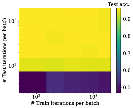
E.4 Dependence on number of iterations

We seek to understand how the performance of our models depends on different levels of compute at train and test time. We train replicas of the convolutional factor graph model (summarised in Table E1) on MNIST, each with a different number of GBP iterations per training batch. We then evaluate the test accuracy of each of the trained models multiple times: for differing numbers of test time GBP iterations. All configurations used a batch size of $200$. We ran our experiments with $50,100,200,400,800,1600$ iterations per batch at both train time and test time. However, we found training with $50$ iterations per batch diverged, so this is not included in the results.

The results are presented in Fig. E1. They show that good test time performance can be achieved with relatively few GBP iterations per batch ($\sim 100$), as long as a sufficient number of iterations is run at test time ($\geqslant 200$).

Figure E1: Dependence of MNIST test accuracy on the number of GBP iterations at train and test time.