Towards cosmology with Void Lensing: how to find voids sensitive to weak-lensing and numerically interpret them

Abstract

ZOBOV| void finder and find significantly deeper weak-lensing profiles for voids defined by our algorithm in the context of a realistic galaxy mock. Then we test the consistency between the measurements of the ESMD as measured through the shear of background galaxies and directly calculated through the dark matter density profiles of the same voids. We found inconsistencies for voids with diameter $\geq 100h^{-1}\mathrm{Mpc}$ along the line-of-sight, but the consistency holds for smaller voids, meaning that we are indeed probing the underlying dark matter field by measuring the shear around these voids. Moreover, we show that voids found in the projected slices, which are highly sensitive to lensing, are correlated to $3$D voids exhibiting intrinsic alignments between them.

ZOBOV| algorithm [13, 12], and the one that we introduce in this work. We show that it is worth exploring the different sensitivity of these different approaches to cosmology and modified gravity, due to the very distinct profiles of voids that they yield. We also investigate the consistency between the VL signal as measured through shear, and the same signal as estimated directly using the DM field. If we aim to do precision cosmology with this observable, we have to, first of all, be sure that we really measure the projected void profile through the shear in a controlled environment. As we will show, when working with voids to measure the ESMD, problems related to the size of voids might arise. We believe this work paves the way for a numerical interpretation of void lensing and therefore for precision cosmological analysis using the data from up-coming surveys with large sky-fraction coverage. This work is organized as follows. In section 1, we briefly review the weak lensing basics. In section 2, we describe the void-finding algorithm introduced in this work, as well as the resulting profile and abundance of voids measured in a simulation. In section 3, we compare the performance of our void-finding algorithm with the widely used ZOBOV void finder by measuring the ESMD in a galaxy mock. In section 4, we compare the ESMD as measured through the tangential shear $\gamma_{t}$ and the one measured directly from the DM field of the same realisation, giving then a numerical interpretation of the observational ESMD and addressing the issue of the thin-lens approximation in the context of void lensing. Finally, we conclude with some observational considerations and avenues for future works.

1 Weak-Lensing theory

In this section, we briefly review a few results of the weak-lensing theory that constitute the basis of this work. We refer to [22] for an extensive review. As the light of background galaxies propagate through LSS, its path is perturbed by the gravitational field in the foreground. The difference between the unperturbed and observed positions, respectively $\boldsymbol{\beta}$ and $\boldsymbol{\theta}$, is given by the lens equation:

$$\boldsymbol{\beta}=\boldsymbol{\theta}-\boldsymbol{\alpha}\,.$$ (1.1)

Assuming small scalar perturbations to the Minkowsky metric, $\boldsymbol{\alpha}$ is given by the projection of the gradient of the gravitational potential along the line of sight:

$$\boldsymbol{\alpha}=\frac{2}{c^{2}}\int^{\chi_{S}}_{0}d\chi^{\prime}\frac{(\chi_{S}-\chi^{\prime})\chi^{\prime}}{\chi_{S}}\boldsymbol{\nabla}_{\perp}\Phi(\boldsymbol{\theta}\chi^{\prime},\chi^{\prime}).$$ (1.2)

The integral is accounting for all lenses at positions $\chi^{\prime}$ up to the source position $\chi_{S}$. The factor $(\chi_{S}-\chi)\chi/\chi_{S}$ is a geometrical weight of the projection. Therefore, it is expected that the observed shapes of background galaxies will be different than the original shapes. The distortion in those shapes is expressed by the distortion matrix

$$A_{ij}=\frac{\partial\beta_{i}}{\partial\theta_{j}}=\delta_{ij}-\frac{\partial\boldsymbol{\alpha}}{\partial\theta_{j}}=\delta_{ij}-\frac{\partial^{2}\psi}{\partial\theta_{i}\partial\theta_{j}},$$ (1.3)

which can be written as

$$\boldsymbol{A}=\begin{pmatrix}1-\kappa-\gamma_{1}&-\gamma_{2}\\ -\gamma_{2}&1-\kappa+\gamma_{1}\par\end{pmatrix}.$$ (1.4)

In eq. 1.3 we have defined the lensing potential

$$\psi=\frac{2}{c^{2}}\int^{\chi_{S}}_{0}d\chi^{\prime}\frac{(\chi_{S}-\chi^{\prime})}{\chi_{S}\chi^{\prime}}\Phi(\boldsymbol{\theta}\chi^{\prime},\chi^{\prime}).$$ (1.5)

The convergence, $\kappa$, is related to the increase or decrease of the overall image size, whereas $\gamma_{1,2}$ parameterize the deviation of the image from a circle and are given by $\gamma_{1}=1/2(\partial_{1}\partial_{1}-\partial_{2}\partial_{2})\psi$, $\gamma_{2}=\partial_{1}\partial_{2}\psi$. Using the previous results, the convergence ($\kappa=1/2(\partial^{2}_{1}+\partial^{2}_{2})\psi$) can be written as

$$\kappa=\frac{1}{4\pi G}\int^{\chi_{s}}_{0}\frac{\nabla^{2}\Phi}{\Sigma_{c}}\mathrm{d}\chi,$$ (1.6)

where $\Sigma_{c}=c^{2}\chi_{S}/(4\pi G\chi(\chi_{S}-\chi))$ is the critical surface mass density. The tangential ($E$ mode) and cross ($B$ mode) components of the shear are defined respectively as $\gamma_{t}=-\mathbb{R}[\gamma e^{-2i\phi}]$ and $\gamma_{\times}=-\mathbb{I}[\gamma e^{-2i\phi}]$, where $\gamma=\gamma_{1}+i\gamma_{2}$. Notice that by factorizing out the convergence in Eq. 1.4, the deviation from identity becomes the reduced shear $g=\gamma/(1-\kappa)$, which is the actual observable. In the weak field regime (our case), $g\simeq\gamma$ is a reasonable approximation. The tangential shear $\gamma_{t}$ is positive in the case in which the foreground lenses are overdensities and negative in the case of underdensities, whereas the cross-component, $\gamma_{\times}$, is related to curl, which is not produced by weak-lensing and therefore must vanish. In the case of axially symetric lenses, we can write the tangential shear in terms of the convergence as

$$\gamma_{t}(r_{\perp})=\bar{\kappa}(<r_{\perp})-\kappa(r_{\perp}),$$ (1.7)

where

$$\bar{\kappa}(<r_{\perp})=\frac{2}{r_{\perp}^{2}}\int^{r_{\perp}}_{0}r_{\perp}^{\prime}\kappa(r_{\perp}^{\prime})dr_{\perp}.$$ (1.8)

In this work, we are interested in measuring the projected profile of voids in the thin lens approximation. Therefore, we take $\Sigma_{c}$ out of the integral in Eq. 1.6, and integrate only in the radial bin that we regard as acting as a thin lens. By inserting the Poisson equation $\boldsymbol{\nabla}^{2}\Phi(\boldsymbol{\theta}\chi,\chi,a)=4\pi Ga^{2}\bar{\rho}_{m}(a)\delta(\boldsymbol{\theta}\chi,\chi)$, the convergence then becomes

$$\kappa=\frac{3H^{2}_{0}\Omega^{(0)}_{m}}{8\pi G\Sigma_{c}}\int^{\chi_{l}+\Delta\chi/2}_{\chi_{l}-\Delta\chi/2}\frac{\delta(\boldsymbol{\theta}\chi,\chi)}{a(\chi)}\mathrm{d}\chi,$$ (1.9)

where $\Delta\chi$ is the bin width in comoving distance, which we consider as a thin lens. Based on this approximation, we define the ESMD in terms of the tangential shear, which is the quantity that we can measure in photometric surveys :

$$\Delta\Sigma(r_{\perp})=\Sigma_{c}\gamma_{t}(r_{\perp}).$$ (1.10)

On the other hand, we can directly calculate the ESMD as

$$\Delta\Sigma(r_{\perp})=\bar{\Sigma}(<r_{\perp})-\Sigma(r_{\perp}),$$ (1.11)

where

$$\Sigma(r_{\perp})=\frac{3H^{2}_{0}\Omega^{(0)}_{m}}{8\pi G}\int^{\chi_{l}+\Delta\chi/2}_{\chi_{l}-\Delta\chi/2}\frac{\delta_{v}(\boldsymbol{\theta}\chi,\chi)}{a(\chi)}\mathrm{d}\chi$$ (1.12)

and

$$\bar{\Sigma}(<r_{\perp})=\frac{2}{r^{2}_{\perp}}\int^{r_{\perp}}_{0}dr^{\prime}_{\perp}r^{\prime}_{\perp}\Sigma(r^{\prime}_{\perp}).$$ (1.13)

In the context of this work we use the void density contrast, $\delta_{v}$, to calculate $\Delta\Sigma$.

2 Optimum Centering Void Finder (OCVF)

In this section we present the void finder algorithm we developed for this work. First we give the intuition and the recipe. Then we show two void statistics produced by this algorithm applied to a N-body simulation: the void density profile and the void abundance.

2.1 Intuition and recipe

In order to have an intuition for how a void finder algorithm should be to deliver an ideal VL profile , we explore the possibilities of VL signals produced by voids described by an hyperbolical tangent-like profile:

$$\delta_{v}(r|R_{v})\equiv\frac{\rho_{v}\left(r\mid R_{v}\right)}{\bar{\rho}_{m}}-1=|\delta_{c}|\left\{\frac{1}{2}\left[1+\tanh\left(\frac{y-y_{0}}{s\left(R_{v}\right)}\right)\right]-1\right\},$$ (2.1)

where $y=\ln(r/R_{v})$, $y_{0}=\ln(r_{0}/R_{v})$, $R_{v}$ is the void radius and $r_{0}=0.37s^{2}+0.25s+0.89$, which is calibrated to describe voids with average density which is $\bar{\rho}_{v}(<R_{v})/\bar{\rho}_{m}=0.2$ of the average density of the Universe, where

$$\bar{\rho}_{v}(<R_{v})=\frac{3}{r^{3}_{v}}\int^{R_{v}}_{0}drr^{3}\bar{\rho}_{m}(\delta_{v}(r)+1),$$ (2.2)

$s$ parameterises the gradient of the profile and $\delta_{c}$ the density contrast at the void center. This profile was first introduced in [23]. We choose to use this profile instead of the widely used HSW profile [24] because the latter has more free parameters and therefore would make this exercise more complicated. However, it is important to notice that the HSW is more general than the profile 2.1, which is particularly suitable in our case. This exercise will give us an intuition for what kind of voids we have to pursue in order to maximize certain desirable properties, namely the signal amplitude and emptiness, since emptier regions are more sensitive to the kind of physics we are interested in when working with voids, namely modifications to gravity, neutrino masses, or complementary information from underdensities which will increase the constraining power in a multi-tracer analysis. Comparisons between different types of void finders was made in the context of N-body simulations by [25], where they found that voids found in the projected DM field have more power of distinguishing between modified gravity and GR. Also, [21] shows that the same type of voids provide the highest S/N. However, the void finder (called Tunnels) which presents the desirable features in both works have overlapping between the voids. Our algorithm is intended to have similar voids but without overlapping, which is desirable in order to be able to predict the theoretical void abundance [26]. Figures 1 and 2 show, respectively, the void density profiles (left) and the corresponding VL profile (right) using Eq. 1.11, when one varies the parameter $s$ (with fixed $\delta_{c}$) and the density at the void center $\delta_{c}$ (with fixed $s$) in the hyperbolical tangent profile ( Eq. 2.1). By Fig. 1 it is clear that voids with profiles that go faster from their minimum density to the average density $\bar{\rho}_{m}$ (smaller $s$) produce deeper VL profiles, with minimum at the void radius, which means that these voids are emptier inside. Figure 2 shows that voids less dense in their centers also produce deeper profiles. Therefore the void finder must satisfy two criteria for defining each void in the catalogue: (i) the voids must have the smallest possible value of density at the center, $\delta_{c}$ (ii) their central position must be as far as possible from overdensities. The criteria (i) can be satisfied by the usage of Delaunay triangulation to define void center candidates. The Delaunay triangulation is a set of d-symplexes (triangules for d = 2 or thetrahedrons for d = 3) $\mathbb{D}(\boldsymbol{P})$ defined in a set of discrete points $\boldsymbol{P}$, such that no point in $\boldsymbol{P}$ is inside any cirum-hypersphere of $\mathbb{D}(\boldsymbol{P})$. In the case d = 2, the Delaunay triangles are those which are circumscribed by circles devoided of any point in $\boldsymbol{P}$ in their interior. In our context, the discrete set $\boldsymbol{P}$ can be any discrete tracer of LSS. By defining void positions as the centers of circum-hyperspheres, or circles circumscribed in Delaunay triangles in d = 2, we guarantee that criteria (i) is being satisfied. The criteria (ii) means that it is not enough to define void positions in empty regions, but also that amongst all the void position candidates we must choose the one which is further away from overdensities. This idea is based on the intuition that voids are empty regions surrounded by walls, filaments and clusters, all of which are overdense structures. Therefore, there is a point for each underdense region which must be further away from these structures. Having all the candidates from the Delaunay triangulation, the point we are looking for is the one from which we can grow the largest possible circle (for d = 2) until it reaches a certain fraction of the average density of the Universe, $\bar{\rho}_{v}(<R_{v})$, which is a free parameter of the void finder. Since all the candidates will have the same average density defined by $\bar{\rho}_{v}(<R_{v})$, the largest is the one which satisfies criteria (ii). Hence the algorithm can be roughly expressed in three steps:

• Perform the Delaunay triangulation to obtain the set of points which are candidates as void positions

• Grow circles (or spheres) around them until the average density of these circles reach a certain density threshold, specified by $\bar{\rho}_{v}(<R_{v})$.

• The largest circle will be the first void in the catalogue and all the other voids which intercept it will be discarded. The same process will be repeated for the second largest remaining void. This process will be repeated until a void which has radius smaller than the cutting radius $R_{c}$ is included in the catalogue.

The value of the cutting radius $R_{c}$ is arbitrary and can be regarded as a free-parameter. This algorithm also captures the “essence” of the excursion set theory [26], since it is a way of finding the voids which correspond to the trajectories which first cross the threshold for void formation.

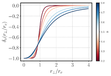
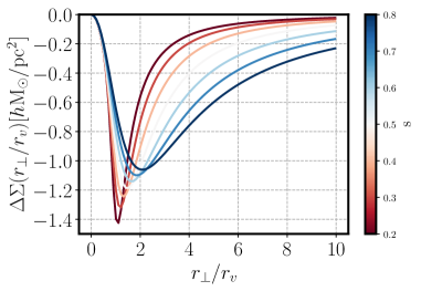
Figure 1: Left: Generic void profiles of type eq. 2.1 for different choices of $s$, which controls the profile gradient. Right: the resulting differential surface densities, $\Delta\Sigma$ obtained through eq. 1.11. This exercise shows that deeper $\Delta\Sigma$ profiles are produced by voids with density profiles which have drastic transitions between $\delta_{c}$ and the average density, $\bar{\rho}_{m}$.

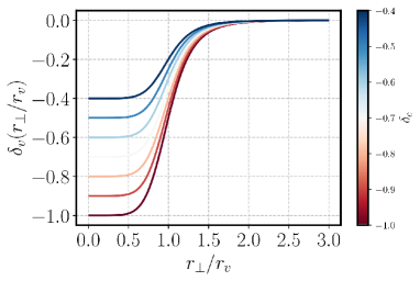
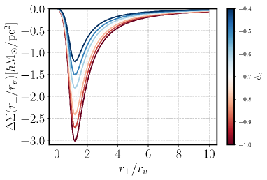
Figure 2: Left: Generic void profiles of type eq. 2.1 for different choices of $\delta_{c}$, which controls the density at the void center position. Right: the resulting differential surface densities, $\Delta\Sigma$ obtained through eq. 1.11. This exercise shows that voids with smaller values of density at its center, $\delta_{c}$ produces deeper differential surface densities, $\Delta\Sigma$.

2.2 Void profile and abundance

In this section, we present the resulting void profiles and abundance after applying the algorithm described in the last section to an N-body simulation. The simulation we use in this section is a $1h^{-1}\textrm{Gpc}$ DM only box from the MultiDark suite [27]. The simulation has $3840^{3}$ DM particles which we sub sampled to have a density of 1 $h^{3}\textrm{Mpc}^{-3}$. The cosmology in this simulation is $(h,\Omega_{\Lambda},\Omega_{m},\Omega_{b},n,\sigma_{8})=(0.67,0.69,0.307,0.048,0.96,0.82)$.

Void Profile

We apply the algorithm to the simulation in its 3D version. For the purpose of visualisation, we show in Fig. 3 the voids found in a 2D slice of 50 $h^{-1}\mathrm{Mpc}$. It is clear that voids are well fitted in underdense regions surrounded by filaments and walls, specially the largest voids. Although we don’t show the same feature in the 3D field, we expect the same result, since the algorithm is exactly the same.

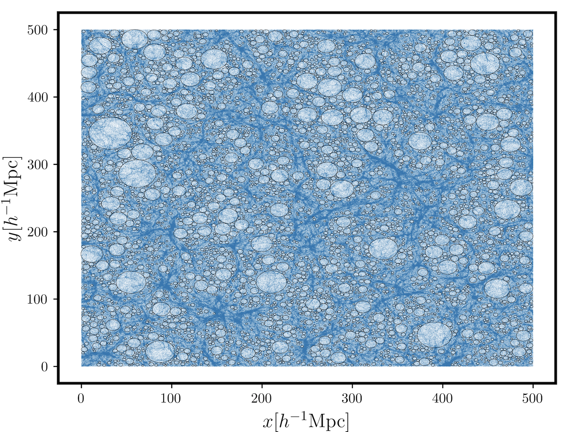
Figure 3: Visualisation of voids found in the projection of a slice of 50 $h^{-1}$Mpc of DM particles.

We can understand how voids are on average by looking at their stacked profiles, i.e $\delta_{v}(r^{\prime})=\rho_{v}(r^{\prime})/\bar{\rho}_{m}-1$, where $r^{\prime}\equiv r/R_{v}$ and $\rho_{v}$ is the density averaged over a spherical shell at reduced distance $r^{\prime}$ to the void center. Figure 4 shows the measured void profiles (black dots), compared to the fit profile given by Eq. 2.1 (dashed-blue). We fit the free parameter $s$ in each bin of radius $R_{v}=\{[3,4],[4,5],[5,6],[6,7],[7,8],[8,9],[9,10],[10,12]\}$ obtaining $s=\{0.38,0.4,0.46,0.48,0.51,0.52,0.53,0.54\}$, meaning that the smallest voids goes from the minimum density to $\delta_{c}=-1$ slightly faster than large voids. The reason for this is that smaller voids are mainly found inside overdense regions, being “voids-in-clouds” [26], they don’t present internal structure but rather they are simply almost empty places in the process of being collapsed by the overdense surroundings. In contrast, the largest voids present more substructures (this can be clearly seen in Fig. 3), smoothing out their profiles. The density profiles do not present a compensation wall such as the ZOBOV voids [28]. This is directly related to the usage of the Delaunay approach that defines void center positions in empty places, and the OCVF post-processing, where only the largest void in every region is kept and all the intercepting ones are discarded. This approach selects voids better placed into the “holes” in LSS. Consequently, the averaged density profile will not present the compensation wall - a signature of overdensities nearby void center positions. It is important to notice that these voids will not be more useful than the ZOBOV ones, but will simply be different tracers of LSS.

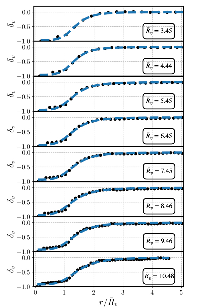
Figure 4: The measured 3D void profiles, $\delta_{v}=\rho_{v}/\bar{\rho}_{m}-1$ for each bin of radius compared to the profile given by Eq. 2.1 [23]. The radii are given in units of $h^{-1}\mathrm{Mpc}$.

Void Abundance

The void abundance (void mass function, or void radius function) is the void analog of mass function for halos, i.e., the counts of objects per bin of mass. Several works have demonstrated its usefulness as a cosmological probe. For instance, [9] and [29] show the sensitivity of the abundance to modifications of gravity, [30] and [5] to massive neutrinos and [31] to alternative dark energy scenarios. Recently, the first cosmological constraints using the void abundance was obtained by [32]. The theory involved in the prediction of the void abundance is analogous to the theory developed for the halo mass function, which goes back to the pioneering work of Press-Schechter [33] and its further developments (e.g. [34, 35, 36]). In the following, we briefly review the theory behind the prediction of the halo mass function. For a complete review, see reference [37]. The so-called excursion set theory is based on the spherical collapse (expansion for voids), in which an isolated overdensity (underdensity) embedded into an Einstein de-Sitter background evolves and eventually collapses and virializes for halos, or experiences shell-crossing between internal shells which expand faster than outer shells for voids. Then, the linearly extrapolated value (from the initial conditions) of the density contrast for which the virialization (shell crossing) occurs is used as a threshold to define a halo (void). These values are $\delta_{c}=1.686$ and $\delta_{v}=-2.7$, for halos and voids. In the excursion set, the Lagrangian density field is smoothed at some scale $R$ as

$$S(R)\equiv\sigma^{2}(R)=\left\langle\delta^{2}(x,R)\right\rangle=\int\frac{d^{3}\boldsymbol{k}}{(2\pi)^{3}}P_{L}(k)W_{R}^{2}(k),$$ (2.3)

where $P_{L}(k)$ is the linear power spectrum and $W_{R}(k)$ is a smoothing function. The smoothed field $\delta(S)$ is then taken to perform a random walk, starting from $S=0$ $(R\rightarrow\infty)$. The excursion set predicts the fraction of walks which will cross the threshold $\delta_{c}$ for the first time in the bin of mass $[M,M+dM]$, $f(M)$. This fraction is then converted into the number density of objects per bin of mass as

$$\frac{dn}{d\ln M}\equiv\frac{d^{2}N}{dVd\ln M}=\bar{\rho}_{m}f(M).$$ (2.4)

The exact form of the function $f(M)$ depends on assumptions regarding the smoothing function $W_{R}(k)$. The most popular choice, which simplifies the calculations, is a sharp-$k$ function [34]. For this choice, the random walk performed by $\delta(S)$ is Markovian and then the probability that a walk first crosses the barrier $\delta_{c}$ is easily obtained as a solution of the Fokker-Planck equation with an appropriate boundary condition [36]. In this case, the halo mass function is given by

$$\frac{dn}{d\ln M}=\frac{\bar{\rho}_{m}}{M}f_{h}(\nu)\frac{d\ln\sigma^{-1}}{d\ln M},$$ (2.5)

where $\nu=\delta_{c}/\sigma$, and the multiplicity function for halos $f_{h}$ is defined as (in the Press-Schechter formalism)

$$f_{h}(\nu)=\sqrt{\frac{2}{\pi}}\nu e^{-\nu^{2}/2}\,.$$ (2.6)

The prediction for the void abundance is analogous and was first proposed by [26]. The main difference from the halo case is the need for two density barriers, $\delta_{c}$ and $\delta_{v}$. So the problem reduces to finding the fraction of walkers which first cross $\delta_{v}$, without having never crossed $\delta_{c}$ for smaller $S$ (larger $R$). The solution obtained in [26] is

$$\frac{dn_{v}}{d\ln R_{L}}=\frac{f^{2SB}_{v}(\sigma)}{V(R_{L})}\frac{d\ln\sigma^{-1}}{d\ln R_{L}},$$ (2.7)

with the void multiplicity function given by

$$f_{v}^{2SB}(\sigma)=2\sum_{n=1}^{\infty}\frac{n\pi}{\delta_{T}^{2}}S\sin\left(\frac{n\pi\delta_{v}}{\delta_{T}}\right)\exp\left(-\frac{n^{2}\pi^{2}}{2\delta_{T}^{2}}S\right).$$ (2.8)

In the above equations $\delta_{T}=|\delta_{v}|+\delta_{c}$, the subscript $L$ and the superscript $2\mathrm{SB}$ stands for , respectively, the linear radius and two static barriers. This radius is the linear comoving radius of the encompassing region in the Lagrangian space, which will expand until the shell crossing (non-linear radius). At the shell crossing, the void has expanded by a factor of $\simeq 1.7$ (see [38]). The two static barriers refer to the density thresholds used in the excursion set, which are constant lines $\delta(S)=\delta_{c},\delta_{v}$. In reference [39], it was noticed that the cumulative fraction of the number of voids exceeds unity. This was interpreted as a brake in the void number conservation. The solution given by Jennings et al. [39] was to impose the conservation of the volume fraction:

$$V(r)dn=V(r_{L})dn_{L}|_{r_{L}(r)}.$$ (2.9)

where the linear and non-linear radii are related as $r\simeq 1.7r_{L}$. Then the void abundance becomes

$$\frac{dn_{v}}{d\ln R}=\frac{f^{2SB}_{v}(\sigma)}{V(R)}\frac{d\ln\sigma^{-1}}{d\ln R_{L}}.$$ (2.10)

In the second paper of the series [36], the static barrier for halo formation was generalised to a stochastic barrier. The stochastic barrier captures the arbitrariness involved in the halo/void finders, as well as complications which arise from environmental conditions. These might act against or in favour of halo/void formation and hence the critical density $\delta_{c}$/$\delta_{v}$ varies depending on the local variance. In [26], an extended excursion set was first presented, i.e. the prediction for the abundance using two linear diffusing barriers:

$$f_{v}^{2\mathrm{LDB}}(\sigma) =2\left(1+D_{v}\right)\exp\left[-\frac{\beta_{v}^{2}\sigma^{2}}{2\left(1+D_{v}\right)}-\frac{\beta_{v}\delta_{c}}{1+D_{v}}\right]$$ (2.11)

$$\times\sum_{n}\frac{n\pi}{\delta_{T}^{2}}\sigma^{2}\sin\left(\frac{n\pi\delta_{c}}{\delta_{T}}\right)\exp\left[-\frac{n^{2}\pi^{2}\left(1+D_{v}\right)}{2\delta_{T}^{2}}\sigma^{2}\right].$$

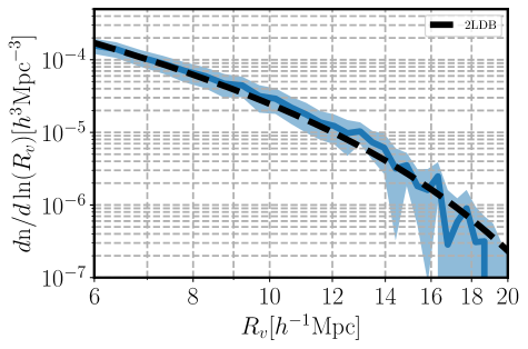
Figure 5: The measured abundance in a DM only N-body simulation of size $L=500h^{-1}\mathrm{Mpc}$ compared to the $2\mathrm{LDB}$ model prediction using two free-parameters ($\beta_{v}$, $D_{v}$).

The superscript in $2\mathrm{LDB}$ stands for two linear diffuse barriers and ($\beta_{v}$, $D_{v}$) are free parameters which describe, respectively, the slope and the diffusive coefficient of the barriers (see [8] for more details). Notice that we use the same slope and diffusive coefficient for the two barriers. The values of the linearly extrapolates thresholds for halo and void formation are kept fixed in $(\delta_{c}=1.686,\delta_{v}=-2.7)$. Figure 5 shows the agreement between the abundance measured in the DM only simulation with size $L=500h^{-1}\mathrm{Mpc}$ and the prediction given by the 2LDB prediction, with best fit free-parameters ($\beta_{v}=0.02,D_{v}=0.2$). The error bars are estimated by splitting the 1Gpc in 8 subboxes, estimating the abundance in each subbox and performing a JK in these 8 samples. The measured abundance is compatible with the theoretical expectation with only 2 free-parameters.

3 Void lensing on galaxies

In this section we compare our algorithm OCVF to ZOBOV (ZOnes Bordering On Voidness algorithm) [28] in the context of void lensing. This algorithm is applied through the wrapper Revolver [40]. We apply both algorithms to the Buzzard mock [41, 42, 43, 44], which models the observed spectroscopic redshifts of galaxies matching a DESI-like survey (DeRose et al. (in prep)). The simulated light-cone covers $10,313.25$ $deg^{2}$, and contains 5,434,414 (BGS) galaxies brighter than $r=20.2$ distributed over the redshift range $z\in[0.1,0.3]$. These galaxies are used as lenses, i.e., we find the voids using them as tracers. The source galaxy catalogue is modelled to match the photometric redshifts of a DES-like survey, occupying the same surface area, with density of 4.4 galaxies/arcmin² in the redshift range $z\in[0.5,1.5]$. The main difference between the ZOBOV and OCVF is that the latter is Delaunay based, whereas the former is Voronoi based. Moreover, here we use the $2$D version of OCVF and ZOBOV finds voids in $3$D.

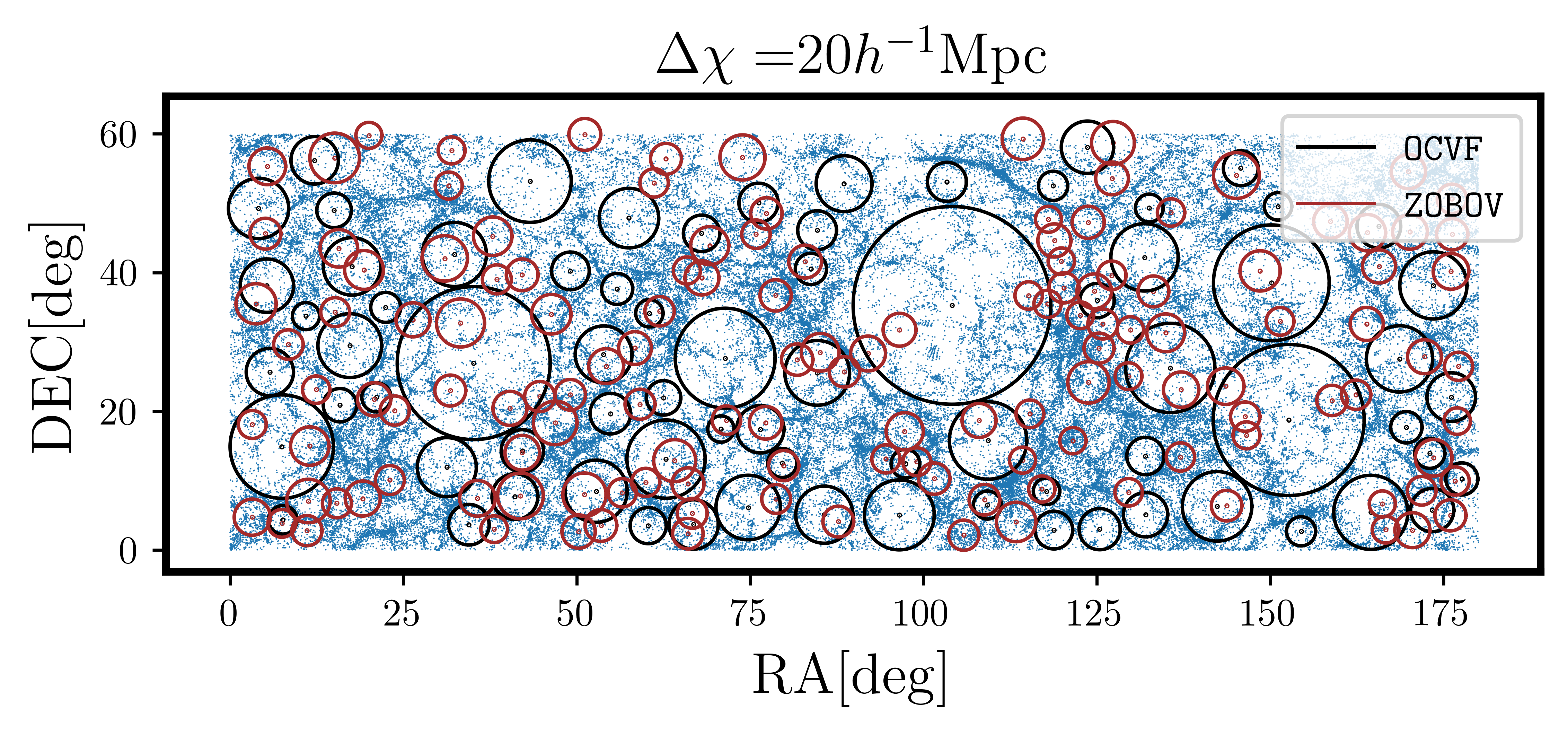
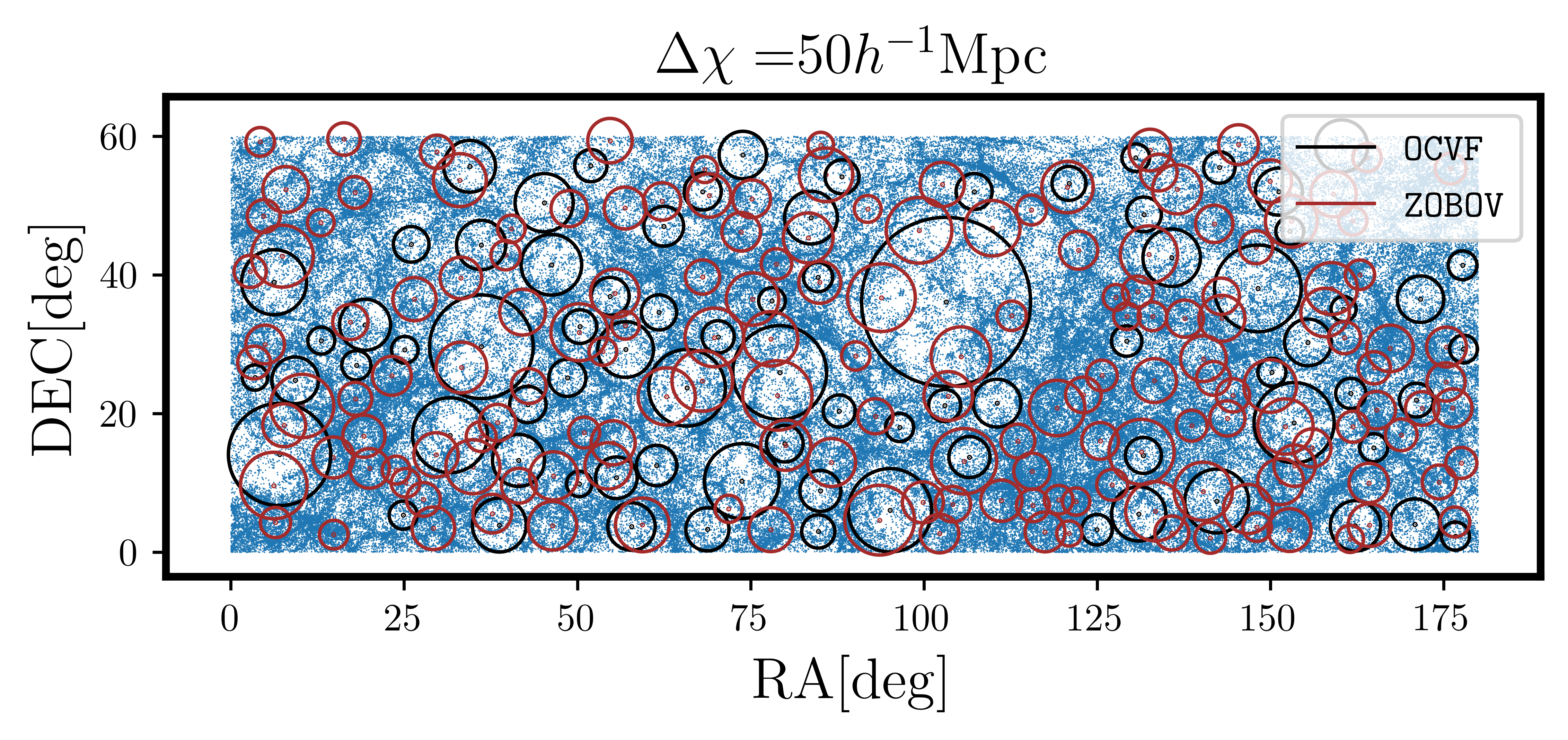
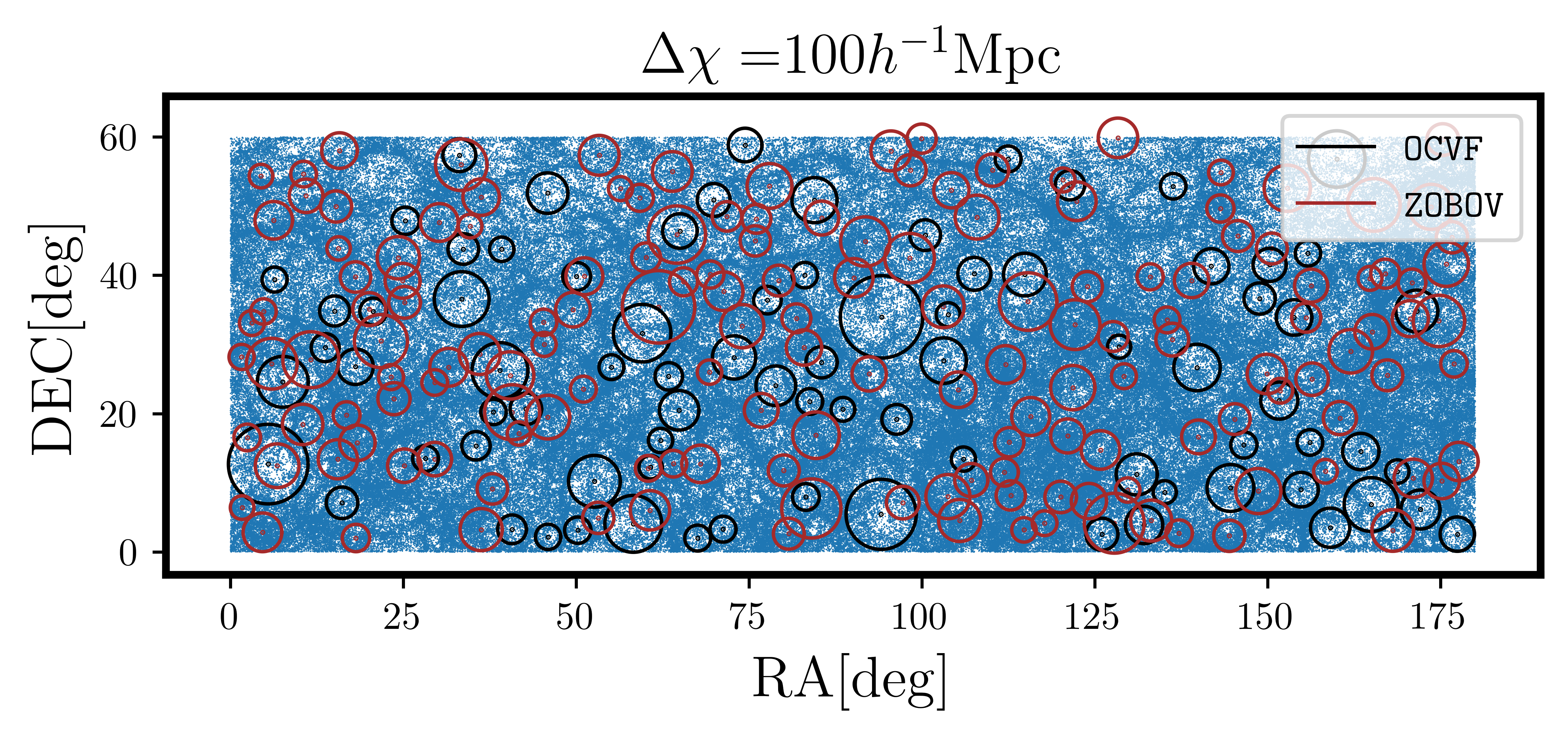
Figure 6: Visualisation of OCVF| and ZOBOV| voids plotted over BGS galaxies, in slices of widths $\Delta\chi=20,$ $50$ and $100[h^{-1}\textrm{Mpc}]$. The ZOBOV| voids were chosen to have their central positions well within the slices.

We chose to show the comparison between the $2$D OCVF because former works have indicated that voids found in projected fields are more efficient at measuring the weak-lensing signal by voids [21] and more sensitive to modifications to gravity [25]. We confirmed that by using the same algorithm to find voids in the 2D and 3D fields, the former provides a signal with larger amplitude. The reason for this is that underdensities in the projected field correspond to anisotropic underdensities in the 3D field, with major-axis aligned with the line-of-sight, as shown in 4.1. As a consequence, the photon’s path is guaranteed to be deviated by underdensities over a greater distance. In contrast, 3D voids are, in general, surrounded by overdensities, which partially or completely erase the signature of overdensities in the photon’s path. This comparison aims to highlight the qualitative differences between these two approaches, which evidences that unlike other statistics, the choice of void finder and how it is applied to data (in the 3D or 2D field, for instance) can drastically change the estimated observable ($\Delta\Sigma$ in this case).

3.1 Void catalogues

The OCVF is applied to the light-cone by splitting it in slices of equal widths along the line of sight. We use the widths $\Delta\chi=20,50,100h^{-1}\mathrm{Mpc}$. Therefore, voids are initially detected as underdensities in projected slices, which in fact correspond to voids in the 3D field as we will discuss in section 4.1. The ZOBOV algorithm is applied to the $3$D galaxy field. The void radius distributions in each version of OCVF (slice width), as well as in ZOBOV are shown in Figure 7. Table 1 shows the total number of voids for each algorithm. We choose to apply a radius cut $R_{v}>10h^{-1}\mathrm{Mpc}$ in all void catalogues. This choice is related to the minimum resolution we have in the galaxy field, but is rather conservative, especially for the OCVF sample, which has the vast majority of voids with radii smaller than $10h^{-1}\mathrm{Mpc}$. However, we believe that these smaller voids are predominantly spurious, i.e. does not correspond to real underdensities in the DM field or are mostly voids-in-clouds. The OCVF voids found in larger slices are significantly less numerous than those found in smaller slices, however, if we normalize the curves to be integrated to unity, all histograms have the same shape. Figure 6 shows the visualisation of ZOBOV and OCVF voids plotted over the BGS galaxy distribution. The chosen ZOBOV voids were those with central positions as close as possible from the bin center we used to find the OCVF voids, in a way that these voids must correspond to the underdensities in this projected slice. By visual inspection it is possible to notice that the OCVF voids are better fitted into the regions with less galaxies in the projected field, whereas ZOBOV voids sometimes correspond to those regions but frequently are placed into overdense regions. This is expected, since OCVF finds voids in the projected slices and ZOBOV is applied to the $3$D field. It shows that three-dimensional voids are sometimes erased in the projected field and, as a consequence, won’t be detectable through lensing, or will simply add noise to the estimated VL profile.

3.2 The $\Delta\Sigma$ Estimator and the TL approximation

The ESMD estimator is given by

$$\widehat{\Delta\Sigma}(r_{\perp}/\mathrm{R_{v}})=\frac{\sum_{ij}w_{ij}\Sigma_{c,ij}\gamma_{t,ij}(r_{\perp}/R_{v})}{\sum_{ij}w_{ij}},$$ (3.1)

where $\gamma_{t,ij}$ is the tangential shear in the source galaxy $i$ due to the void $j$. For each pair, the weights that minimize the variance of the signal are $w_{ij}=\Sigma^{-2}_{c,ij}$ [45], and the critical mass density is defined as

$$\Sigma_{c,ij}=\frac{c^{2}}{4\pi G}\frac{\chi(z_{i})}{\chi(z_{j})(\chi(z_{i})-\chi(z_{j}))}.$$ (3.2)

The tangential shear is calculated from the shear components $\gamma_{1,2}$ (defined in section 1 and obtained in [41] through ray-tracing) and the angle $\phi$ between the void and source positions. The estimated ESMD is expressed in terms of the reduced perpendicular distance to the line-of-sight $r_{\perp}/R_{v}$ because voids with different sizes present very similar profiles in reduced coordinates. This is what we mean by stacked void profile. The estimator 3.1 is based under the assumption that the shear $\gamma_{t,ij}$ for all voids can be obtained by assuming the thin lens approximation, in which the net effect on the photons path will depend only on the target structure which can be regarded as being contained in a single plane, i.e. ignoring the line-of-sight direction. In other words, the remaining structures when subtracting the void will have zero net effect on the photons path and the only effect can be computed by projecting the density field of the voids, as in eq. 1.9. In this case the equality in 3.1 is true. However, it is possible that individual voids extend to distances larger than the maximum distance which does not allow us to write that $\Delta\Sigma=\Sigma_{c}\gamma_{t}$. In this case, a systematic error will be introduced in the estimator 3.1.

3.3 Void finder comparison

In Figure 8, we show the measurement of the ESMD performed using voids found in the 3D-galaxy field with the ZOBOV algorithm, as well as voids found in projected fields with the OCVF algorithm. The ZOBOV voids are split into two sub-samples, $R_{v}\in[10,15]$ and $R_{v}\in[10,25]$ ($h^{-1}\mathrm{Mpc}$). The reason why we use these two sub-samples and 25$h^{-1}\mathrm{Mpc}$ as maximum radius is justified in section 4. The OCVF voids are presented in three samples, each of which corresponds to the algorithm applied to slices of widths $\Delta\chi=20,50,100h^{-1}\mathrm{Mpc}$. The right and left plots show, respectively, the tangential ($\Delta\Sigma_{t}$) and cross ($\Delta\Sigma_{\times}$) components. The tangential component presents several differences. Firstly, the ZOBOV voids present a compensation wall, whereas the OCVF does not. The compensation wall is a direct consequence of the same feature in the void’s 3D density profile, which means that these voids are closer to overdensities, whereas OCVF voids are far enough from overdensities to not have correlation with them. Another notorious difference is that ZOBOV voids are shallower. There are two reasons for this. The first is the existence of a compensation wall, which produces positive tangential shear, $\gamma_{t}$. The second reason can be intuitively seen in Figure 6: not all ZOBOV voids correspond to underdensities in the projected field, whereas the voids found in projected fields are guaranteed to not be correlated with overdensities along the line-of-sight. Moreover, larger projected slices tend to select underdensities aligned with the line-of-sight. The OCVF voids are presented in three samples, each of which corresponds to the algorithm applied to slices of widths $\Delta\chi=20,50,100h^{-1}\mathrm{Mpc}$. These voids correspond to 3D underdense structures which have their major axis aligned with the line-of-sight (see Figure 10). In the Appendix B we briefly discuss that not only the voids in the projected field present an anisotropic 3D density profile, but also the subsample voids found using the 3D version of the same algorithm (OCVF), therefore following the theoretical abundance (Figure 5), also present anisotropic 3D density profiles. This subsample is chosen using the distances from the 3D voids to the projected voids which present correlation between them (Figure 14). This result indicates that what we really find by applying the void finder in the projected field are combinations of 3D voids which present intrinsic alignment between them. The cross-components must be consistent with zero. It is almost always satisfied, except in some cases for small $r_{\perp}/R_{v}$, where it is slightly bellow zero. The same feature also appears in the tangential component (it must go to zero as $r_{\perp}/R_{v}\rightarrow 0$). This indicates a systematic error for small $r_{\perp}/R_{v}$ that we do not comprehend.

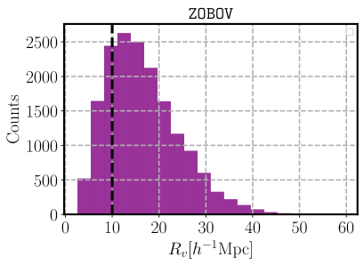
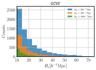
Figure 7: Left: Radius distribution of ZOBOV| voids. Right: Radius distribution of OCVF| voids

In Figure 9 we compare the cumulative signal-to-noise (S/N) of the tangential component, defined as

$$(S/N)^{2}(<r_{\perp,k})=\sum_{i\leq k,j\leq k}\Delta\Sigma_{t,i}C^{-1}_{ij}\Delta\Sigma_{t,j},$$ (3.3)

where $C_{ij}$ is the covariance matrix estimated through a void-by-void jack-knife. The left plot shows the cumulative S/N for each sample, whereas the right plot shows the same quantity normalised by the number of voids in the corresponding sample (Table 1). The cumulative S/N is quite similar for all samples, except for the ZOBOV sample with maximum radius of 15$h^{-1}\mathrm{Mpc}$. The normalised S/N is significantly higher for the OCVF samples corresponding to the slices widths of $\Delta\chi=50,100h^{-1}\mathrm{Mpc}$. This result is expected: the larger is the slice width, the larger is the photon’s path which corresponds to underdensities, i.e., less contamination from overdensities. It should be stressed that this comparison does not assess which sample is more useful to constrain cosmology. Indeed, larger S/N does not necessarily mean more sensitive to cosmological parameters or modifications to gravity. However, we can say that measuring the lensing signal by voids using projected slices and the OCVF will produce a signal which tells more about underdensities than the one obtained using ZOBOV voids. By thinking of voids as being the most underdense tracers of LSS and assuming that tracers with different biases carry complementary information (see e.g. [46, 47]), then the OCVF profiles in Figure 8 have biases more negative than the ZOBOV profiles.

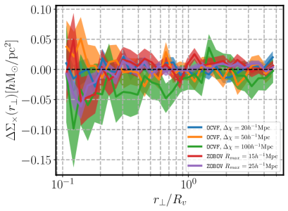
Figure 8: Left: Comparison between the $\Delta\Sigma_{t}$ measurements performed using the OCVF| in slices of width $\Delta\chi=20$, $50$, $100\,h^{-1}\,\mathrm{Mpc}$ (blue, orange, and green) and ZOBOV| in the bins of radius $[10,15]h^{-1}\mathrm{Mpc}$ (red) and $[10,25]h^{-1}\mathrm{Mpc}$ (purple). Right: The same comparison for the cross component $\Delta\Sigma_{\times}$.

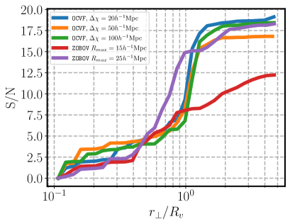
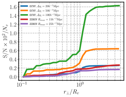
Figure 9: Left: Comparison between the cumulative S/N on $\Delta\Sigma_{t}$ obtained using the OCVF| on slices of width $\Delta\chi=20$, $50$, $100\,h^{-1}\,\mathrm{Mpc}$ (blue, orange, and green) and ZOBOV| (red and purple) in the redshift bin $0.1<z<0.3$. Right: S/N normalized by the number of voids

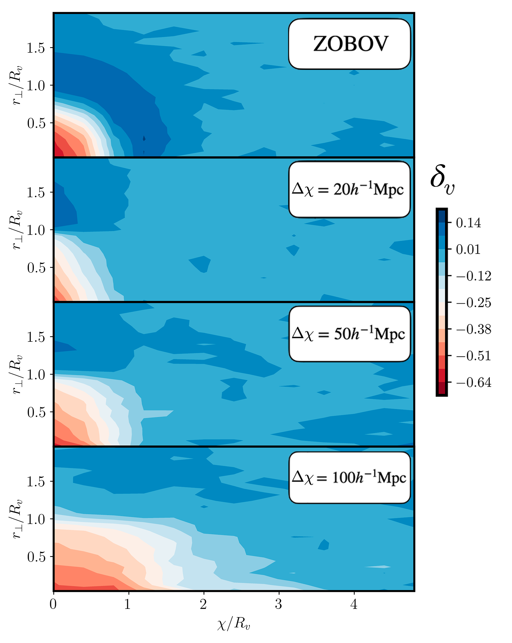
Figure 10: Void DM profiles as a function of radial comoving distance, $\chi/R_{v}$ (centered at the void position) and the perpendicular distance to the line-of-sight, $r_{\perp}/R_{v}$. The top panel shows profiles estimated with ZOBOV| voids found in the 3D galaxy distribution, and the profiles labeled by $\Delta\chi=20,50,100h^{-1}\mathrm{Mpc}$ are OCVF| voids found in slices of labeled sizes.

Void Finder	$N_{v}(0.1<z<0.3)$
OCVF ($\Delta\chi$ = 20 $h^{-1}\textrm{Mpc}$)	7321
OCVF ($\Delta\chi$ = 50 $h^{-1}\textrm{Mpc}$)	2623
OCVF ($\Delta\chi$ = 100 $h^{-1}\textrm{Mpc}$)	1131
ZOBOV	13438

Table 1: The total number of voids for each void finder in the redshift bin $z$ $\in$ $[0.1,0.3]$.

4 Numerical interpretation

Voids are peculiar tracers of LSS and it is not clear whether an analytic approach, based on perturbation theory, or effective field theory of large scale structure would be able to predict their density profiles, i.e., the cross-correlation void-tracer. The main reason for this impossibility is that voids are not uniquely defined, imposing a puzzle on how the condition related to the void center definition will be incorporated in the growth equation, in the case of linear perturbation theory. Therefore, a promising approach to extract this cosmological information is to take their profiles directly from N-body simulations and apply some emulation technique to predict their profiles for a set of cosmologies. In the context of VL, we have the advantage that we can directly use a DM only box to performe the emulation, since this observable is probing directly the total matter field. In this section we pave the way for this kind of approach. We use the DM particles of the same realisation we used in the previous section and estimate the DM profiles of the same voids we found in the galaxy field. Then we use these void DM profiles to check the consistency between the $\Delta\Sigma$ profiles we estimated in the previous section (through the shear of background galaxies), and the same quantity, but estimated directly from the DM field. This consistency test will show whether we are really having access to the DM profiles of these voids through weak-lensing. This consistency test is crucial if we aim to use the VL profile to do precision cosmology in the near future. As we will show, this consistency is not trivially given in the context of voids, as it is in the context of halos.

4.1 VL and Void Dark Matter profiles

Figure 10 shows the stacked void profiles as a function of parallel and perpendicular distances to the line-of-sight, estimated using the DM particles of the Buzzard mock, i.e., the cross-correlation between void centers and DM particles for voids found in the BGS galaxy field:

$$\delta_{v}(r^{\prime}_{\perp},\chi^{\prime})=\frac{1}{N_{v}}\sum^{N_{v}}_{i}\frac{n^{i}_{p}(\Delta r^{\prime}_{\perp},\Delta\chi^{\prime})}{\langle n_{p}\rangle}-1,$$ (4.1)

where $r^{\prime}_{\perp}\equiv r_{\perp}/R_{v}$, $\chi^{\prime}\equiv\chi/R_{v}$ and $\Delta r^{\prime}_{\perp}(\chi)$ denotes a bin in $(r^{\prime}_{\perp},\chi^{\prime})$. Since we are estimating these profiles in configuration space, we expect that they will be isotropic. However, the profiles for increasingly larger slices become increasingly anisotropic. Since only voids aligned with the line-of-sight are detected as voids in the projected field, the resulting stacked profile will be anisotropic and might contain some information encoded in the void ellipticities of voids defined in the 3D distribution (see Appendix B). This can be directly accessed with void lensing measurements. The relation between anisotropic and isotropic profiles is the topic of an ongoing work.

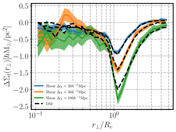
Figure 11: Comparison between $\Delta\Sigma_{t}$ as measured through the shear (blue, orange, and green) and directly using the DM particles (dashed black).

4.2 Consistency between shear and Dark matter density profile around voids

In this section, we check the consistency between the $\Delta\Sigma_{t}$ profile of voids measured from the shear, i.e., $\Delta\Sigma_{t}=\Sigma_{c}\gamma_{t}$ and the one directly calculated using the DM density profiles of voids presented in figure 10. We take the same realisation of the density field, as traced by BGS galaxies. Therefore, we compare the observable we have access through observations against the same observable but computed using the DM field, which we do not have access to in real observations. In the case where this consistency test is successful, we know exactly what we would observe in real data, given that the assumption we are using in simulations are well calibrated w.r.t real data, namely, the galaxy bias and possible systematic effects such as intrinsic alignment and survey mask. Before proceeding, it is important to mention the reasons why the two quantities might differ:

• The impact of the source distribution: In the estimator 3.1, the weights and the $\gamma_{t}$ depend on $\Sigma_{c}$ which contains information about the source distribution. By predicting $\Delta\Sigma_{t}$ only in terms of the void DM profile, without saying anything about the source distribution, it is not clear whether we can recover the same quantity than the one estimated.

• The impact of the thin lens approximation: To quote the results in terms of $\Delta\Sigma_{t}$ we are assuming that the void profile, or everything that will have an impact on the average shape of background galaxies is contained in a thin lens (see eq. 1.9). Since voids can have radius as large as $\simeq 100h^{-1}$Mpc and, furthermore, might have correlations with overdensities beyond the void radius, it is not clear whether the thin lens assumption still holds.

In order to calculate the $\Delta\Sigma_{t}$ profiles from the 3D void profiles in figure 10, we will exclude small scales to avoid resolution effects by using the annular differential surface density (ADSD):

$$\Upsilon\left(R|R_{0}\right)\equiv \Delta\Sigma_{t}(R)-\frac{R_{0}^{2}}{R^{2}}\Delta\Sigma_{t}\left(R_{0}\right)$$ (4.2)

$$= \frac{2}{R^{2}}\int_{R_{0}}^{R}\mathrm{~{}d}R^{\prime}R^{\prime}\Sigma\left(R^{\prime}\right)-\frac{1}{R^{2}}\left[R^{2}\Sigma(R)-R_{0}^{2}\Sigma\left(R_{0}\right)\right],$$

where $R_{0}$ is the cutting scale. For sufficiently small $R_{0}$, $\Upsilon$ reduces to $\Delta\Sigma_{t}$. We checked that the estimated profile does not depend on the particular choice of $R_{0}$, for $R_{0}\leq 0.5$ in reduced coordinate ($r_{\perp}/R_{v}$). Since we are working with stacked void profiles, $\Delta\Sigma$ is proportional to the void radius, which comes from the Jacobian when tranforming the integral from $r^{\prime}_{\perp}$ to $r_{\perp}/R_{v}$ coordinate. Thus,

$$\Sigma(r^{\prime}_{\perp})=R_{v}\Sigma(r_{\perp}),$$ (4.3)

where $\Sigma(r_{\perp})$ is given by eq. 1.12 and, consequently,

$$\Delta\Sigma_{t}(r^{\prime}_{\perp})=R_{v}\Delta\Sigma_{t}(r_{\perp}).$$ (4.4)

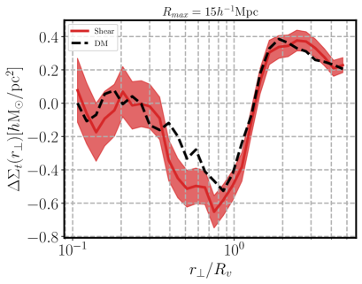
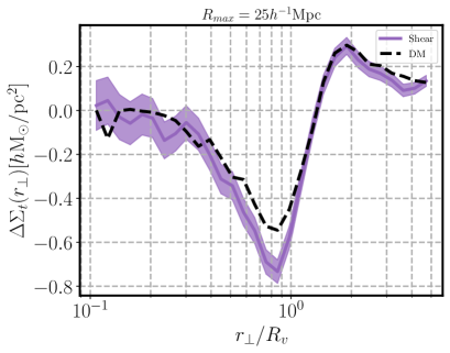
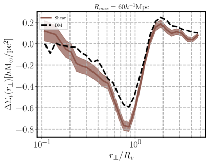
Figure 12: The consistency check between the $\Delta\Sigma_{t}$ estimated through the shear of background galaxies and the same quantity estimated directly from the DM profiles of the same voids. Respectively, the top-left, top-right and bottom plots show the consistency test for ZOBOV| voids with radii in the ranges $[10,15]$, $[10,25]$ and $[10,60]$ in units of $h^{-1}\mathrm{Mpc}$.

Figure 11 shows the results of the same $\Delta\Sigma_{t}$ profiles as shown in figure 8, through the estimator 3.1, against the $\Delta\Sigma_{t}$ estimated using the DM particles around the voids. In this estimation we project the void profiles using a bin width $\Delta\chi^{\prime}$:

$$\Sigma(r_{\perp})=R_{v}\int_{\chi^{\prime}_{l}-\Delta\chi^{\prime}/2.}^{\chi^{\prime}_{l}+\Delta\chi^{\prime}/2.}\frac{d\chi^{\prime}}{a(\chi^{\prime})}\delta_{v}(r^{\prime}_{\perp},\chi^{\prime}).$$ (4.5)

and then compute the ADSD signal using eq. 4.2. We obtain consistency between shear and DM profiles for the OCVF samples computed in slices of widths $\Delta\chi=20,50h^{-1}\mathrm{Mpc}$. However for the sample with $L=100h^{-1}\mathrm{Mpc}$, the two profiles become inconsistent at reduced radius $r^{\prime}_{\perp}\sim 1$. We obtain the same trend for the ZOBOV voids (Figure 12). The subsample in the radius bin [10, 15] ($h^{-1}\mathrm{Mpc}$) is quite consistent, whereas the subsamples including larger voids, namely, [10, 25]($h^{-1}\mathrm{Mpc}$) and [10, 60]($h^{-1}\mathrm{Mpc}$), present increasing inconsistencies. The trend with both void finders is, the larger is the stacked void profile, the larger is the inconsistency between shear and DM profiles. Furthermore, the void size in the direction perpendicular to the line-of-sight seems to be unimportant, since the normalised radius distribution of OCVF voids is the same amongst the different bins widths. We conclude that what really matters for this consistency is the void size along the line-of-sight, which indicates that the thin lens approximation might be broken in the cases in which the correlations between the void and its surroundings extend beyond a certain limit. In the Appendix A we show an example of how a break of the thin lens approximation affects the VL profiles. We use generic analytical void profiles and calculate $\Delta\Sigma$ with and without the thin lens approximation. The wrong assumption of the thin lens approximation tends to underestimate the VL profile, specially around $r_{\perp}/R_{v}\simeq 1$, which is exatly what we see in the DM profiles of Figures 11 and 12. The source of the inconsistency might be, then, the wrong assumption of the thin lens approximation in the estimator 3.1.

5 Conclusions

In this work we have studied the VL profile in the context of galaxy mock. First, we proposed a new void finder algorithm which is particularly designed to deliver voids with deep VL profiles. Then, we apply this algorithm to the galaxy mock and contrast it with the widely used algorithm in literature, ZOBOV. The latter has been used in previous measurements of the VL profile in real data and provided a higher S/N compared to an algorithm similar to ours [13]. We show that, compared to ZOBOV, voids found in projected slices using our algorithm can provide a higher S/N per void, with a deeper VL profile. These voids correspond to combinations of voids in the 3D DM field which present intrinsic alignment between them, suggesting that the VL profile might be sensitive to the void intrinsic alignment. This opens some questions, namely: (i) is the void intrinsic alignment connected to tidal fields in LSS and, therefore, to cosmology? (ii) How sensitive is the VL profile to the intrinsic alignment? Then we checked the consistency between the VL profile as estimated through the shear of background galaxies and the same quantity as estimated directly from the DM density profiles of voids. This consistency test has never been made (up to the knowledge of the present authors) and it is crucial for future cosmological analysis using VL profile as an observable. Unlike halos, voids have density profiles that extend over hundreds of $h^{-1}\mathrm{Mpc}$, which might break the assumption of voids being contained in a thin slice, which is a basic assumption when estimating the VL profile from the shear of background galaxies. Furthermore, voids are much less numerous than halos and therefore residual contributions from structures along the line-of-sight might not be averaged out, as it easily is in the context of halos. This consistency test shows that voids with larger sizes along the line-of-sight present inconsistencies between the shear and DM VL lensing profiles, suggesting that the thin lens approximation assumed in the estimator is not appropriate in the case of voids in general. For ZOBOV voids smaller than $15h^{-1}\mathrm{Mpc}$ and OCVF found in projected slices smaller than $50h^{-1}\mathrm{Mpc}$ the shear and DM VL profiles are consistent. In future works, we plan to further understand the relation between the VL profile around voids in the projected field and the intrinsic alignments of voids in the 3D field. Also, we plan to model the VL profile with dependency on the cosmological parameters. This work paves the way for a trivial numerical prediction: since we have shown that for a suitable choice of void definition, the shear and DM VL profile are consistent, emulation techniques which are becoming widely used in cosmology can be used to interpret real data observations. Is it also important to have an analytical prediction of the VL observable, which is the subject of an ongoing work by the present author.

Appendix A How the thin lens approximation affects the VL profiles

In this appendix we explore the limits of the thin lens approximation, which is relevant in the case of voids, given their large size. As pointed out in section 4, the matching between measured and predicted ESMD depends on whether we can consider voids as thin lenses in between the source and the observer or not, i.e., whether we can write the convergence as eq. 1.9. To test this assumption we use a void profile with similar shape to the stacked profile produced by OCVF to compute $\Delta\Sigma$ with and without the thin lens approximation. We use a “worst case scenario” in which the void position is too close to the source with redshifts $z_{l}=0.48$ and $z_{s}=0.5$, respectively for the void and the source, and vary the void radius $R_{v}=(50,100,150)h^{-1}\mathrm{Mpc}$. The combination of void radius and distance between the source and the void are the variables that control whether the thin lens is a good approximation or not. Figure 13 shows the predictions for the ESMD for different void radius (left) and the relative difference between the same quantity calculated with and without the thin lens approximation (right). This exercise shows that for voids with radius of $50h^{-1}\mathrm{Mpc}$ the difference is below $\simeq 5\%$.

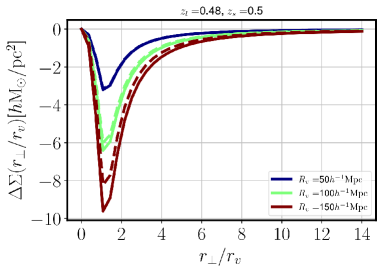
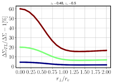
Figure 13: Left: The ESMD profiles for different void radius with (solid) and without (dashed) the thin lens approximation. Right: The relative difference between the ESMD with and without thin lens approximation.

Appendix B The void intrinsic alignment around projected voids

In this appendix we show some preliminary results about the shapes of 3D voids around the voids found in the projected slices that we use in this work. Both void samples were created using the OCVF algorithm. We use the same simulation we used in section 2 to find both void samples. The left plot in Figure 14 shows the correlation between a sample of voids found in projected fields of width $\Delta\pi=50h^{-1}\mathrm{Mpc}$ with radii in the range $8<R^{b}_{v}<15h^{-1}\mathrm{Mpc}$ and the 3D voids in different radius bins. The right plot shows the stacked profile of the 3D voids as a function of the perpendicular, $\sigma$, and parallel, $\pi$, distances to the line of sight. The correlations shows that voids in $3$D and $2$D with similar sizes present stronger correlations. The stacked profiles of the $3$D voids are clearly anisotropic. This shows that $3$D voids around voids found in the projected slices present intrinsic alignment between them, or, equivalently, that the voids found in projected slices are actually the combination of $3$D voids, which are aligned between them. A more detailed study of the correlations and the statistical relation between voids found in projected slices and $3$D voids is the subject of ongoing work.

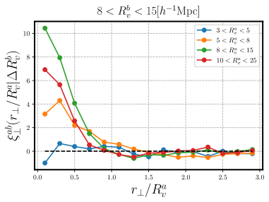
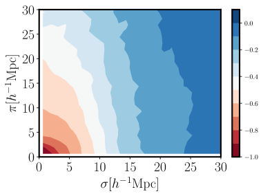
Figure 14: Left: Correlation between voids found in the projected field, labelled by “b” and voids found in the 3D field, labelled by “a”. Right: the stacked profile of 3D voids which are at a distance from the projected voids which presents non-zero correlation, as a function of the parallel, $\pi$, and perpendicular, $\sigma$, distance to the line-of-sight.

References

- [1] R. Laureijs, J. Amiaux, S. Arduini, J. L. Auguères, J. Brinchmann, R. Cole et al., Euclid definition study report, 2011.
- [2] A. Aghamousa, J. Aguilar, S. Ahlen, S. Alam, L. E. Allen, C. A. Prieto et al., The desi experiment part i: science, targeting, and survey design, arXiv preprint arXiv:1611.00036 (2016) .
- [3] K. C. Chan, Y. Li, M. Biagetti and N. Hamaus, Measurement of void bias using separate universe simulations, The Astrophysical Journal 889 (2020) 89.
- [4] A. Pisani, P. Sutter, N. Hamaus, E. Alizadeh, R. Biswas, B. D. Wandelt et al., Counting voids to probe dark energy, Physical Review D 92 (2015) 083531.
- [5] E. Massara, F. Villaescusa-Navarro, M. Viel and P. Sutter, Voids in massive neutrino cosmologies, Journal of Cosmology and Astroparticle Physics 2015 (2015) 018.
- [6] N. Schuster, N. Hamaus, A. Pisani, C. Carbone, C. D. Kreisch, G. Pollina et al., The bias of cosmic voids in the presence of massive neutrinos, Journal of Cosmology and Astroparticle Physics 2019 (2019) 055.
- [7] M. Kamionkowski, L. Verde and R. Jimenez, The void abundance with non-gaussian primordial perturbations, Journal of Cosmology and Astroparticle Physics 2009 (2009) 010.
- [8] R. Voivodic, M. Lima, C. Llinares and D. F. Mota, Modeling void abundance in modified gravity, Physical Review D 95 (jan, 2017) .
- [9] E. L. Perico, R. Voivodic, M. Lima and D. F. Mota, Cosmic voids in modified gravity scenarios, Astronomy & Astrophysics 632 (2019) A52.
- [10] E. Massara and R. K. Sheth, Density and velocity profiles around cosmic voids, arXiv preprint arXiv:1811.03132 (2018) .
- [11] L. Amendola, J. A. Frieman and I. Waga, Weak gravitational lensing by voids, Monthly Notices of the Royal Astronomical Society 309 (1999) 465–473.
- [12] C. Sánchez, J. Clampitt, A. Kovacs, B. Jain, J. García-Bellido, S. Nadathur et al., Cosmic voids and void lensing in the dark energy survey science verification data, Monthly Notices of the Royal Astronomical Society (2016) stw2745.
- [13] Y. Fang, N. Hamaus, B. Jain, S. Pandey, G. Pollina, C. Sánchez et al., Dark energy survey year 1 results: the relationship between mass and light around cosmic voids, Monthly Notices of the Royal Astronomical Society 490 (2019) 3573–3587.
- [14] P. Melchior, P. Sutter, E. S. Sheldon, E. Krause and B. D. Wandelt, First measurement of gravitational lensing by cosmic voids in sdss, Monthly Notices of the Royal Astronomical Society 440 (2014) 2922–2927.
- [15] A. Barreira, M. Cautun, B. Li, C. M. Baugh and S. Pascoli, Weak lensing by voids in modified lensing potentials, Journal of Cosmology and Astroparticle Physics 2015 (2015) 028.
- [16] T. Baker, J. Clampitt, B. Jain and M. Trodden, Void lensing as a test of gravity, Physical Review D 98 (2018) 023511.
- [17] C. T. Davies, M. Cautun and B. Li, Cosmological test of gravity using weak lensing voids, Monthly Notices of the Royal Astronomical Society 490 (2019) 4907–4917.
- [18] T. Shimasue, K. Osato, M. Oguri, R. Shimakawa and A. J. Nishizawa, Line-of-sight structure of troughs identified in subaru hyper suprime-cam year 3 weak lensing mass maps, arXiv preprint arXiv:2307.11407 (2023) .
- [19] D. Gruen, O. Friedrich, A. Amara, D. Bacon, C. Bonnett, W. Hartley et al., Weak lensing by galaxy troughs in des science verification data, Monthly Notices of the Royal Astronomical Society 455 (2016) 3367–3380.
- [20] Y. Higuchi, M. Oguri and T. Hamana, Measuring the mass distribution of voids with stacked weak lensing, Monthly Notices of the Royal Astronomical Society 432 (2013) 1021–1031.
- [21] C. T. Davies, E. Paillas, M. Cautun and B. Li, Optimal void finders in weak lensing maps, Monthly Notices of the Royal Astronomical Society 500 (2021) 2417–2439.
- [22] P. Schneider, Gravitational lenses, in Gravitational Lenses: Proceedings of a Conference Held in Hamburg, Germany 9–13 September 1991, pp. 196–208, Springer, 2005.
- [23] R. Voivodic, H. Rubira and M. Lima, The halo void (dust) model of large scale structure, Journal of Cosmology and Astroparticle Physics 2020 (2020) 033.
- [24] N. Hamaus, P. Sutter and B. D. Wandelt, Universal density profile for cosmic voids, Physical review letters 112 (2014) 251302.
- [25] M. Cautun, E. Paillas, Y.-C. Cai, S. Bose, J. Armijo, B. Li et al., The santiago–harvard–edinburgh–durham void comparison–i. shedding light on chameleon gravity tests, Monthly Notices of the Royal Astronomical Society 476 (2018) 3195–3217.
- [26] R. K. Sheth and R. Van De Weygaert, A hierarchy of voids: much ado about nothing, Monthly Notices of the Royal Astronomical Society 350 (2004) 517–538.
- [27] F. Prada, A. A. Klypin, A. J. Cuesta, J. E. Betancort-Rijo and J. Primack, Halo concentrations in the standard cold dark matter cosmology, Monthly Notices of the Royal Astronomical Society 423 (2012) 3018–3030.
- [28] M. C. Neyrinck, Zobov: a parameter-free void-finding algorithm, Monthly notices of the royal astronomical society 386 (2008) 2101–2109.
- [29] Y.-C. Cai, N. Padilla and B. Li, Testing gravity using cosmic voids, Monthly Notices of the Royal Astronomical Society 451 (2015) 1036–1055.
- [30] C. D. Kreisch, A. Pisani, C. Carbone, J. Liu, A. J. Hawken, E. Massara et al., Massive neutrinos leave fingerprints on cosmic voids, Monthly Notices of the Royal Astronomical Society 488 (2019) 4413–4426.
- [31] G. Verza, A. Pisani, C. Carbone, N. Hamaus and L. Guzzo, The void size function in dynamical dark energy cosmologies, Journal of Cosmology and Astroparticle Physics 2019 (2019) 040.
- [32] S. Contarini, A. Pisani, N. Hamaus, F. Marulli, L. Moscardini and M. Baldi, Cosmological constraints from the boss dr12 void size function, The Astrophysical Journal 953 (2023) 46.
- [33] W. H. Press and P. Schechter, Formation of galaxies and clusters of galaxies by self-similar gravitational condensation, Astrophysical Journal, Vol. 187, pp. 425-438 (1974) 187 (1974) 425–438.
- [34] J. Bond, S. Cole, G. Efstathiou and N. Kaiser, Excursion set mass functions for hierarchical gaussian fluctuations, Astrophysical Journal, Part 1 (ISSN 0004-637X), vol. 379, Oct. 1, 1991, p. 440-460. Research supported by NSERC, NASA, and University of California. 379 (1991) 440–460.
- [35] J. Peacock and A. Heavens, Alternatives to the press–schechter cosmological mass function, Monthly Notices of the Royal Astronomical Society 243 (1990) 133–143.
- [36] M. Maggiore and A. Riotto, The halo mass function from excursion set theory. ii. the diffusing barrier, The Astrophysical Journal 717 (2010) 515.
- [37] V. Desjacques, D. Jeong and F. Schmidt, Large-scale galaxy bias, Physics reports 733 (2018) 1–193.
- [38] G. Blumenthal, L. N. Da Costa, D. Goldwirth, M. Lecar and T. Piran, The largest possible voids, Astrophysical Journal, Part 1 (ISSN 0004-637X), vol. 388, April 1, 1992, p. 234-241. Research supported by USIBSF and Smithsonian Institution. 388 (1992) 234–241.
- [39] E. Jennings, Y. Li and W. Hu, The abundance of voids and the excursion set formalism, Monthly Notices of the Royal Astronomical Society 434 (2013) 2167–2181.
- [40] S. Nadathur, P. M. Carter, W. J. Percival, H. A. Winther and J. E. Bautista, Revolver: Real-space void locations from suvey reconstruction, Astrophysics Source Code Library (2019) ascl–1907.
- [41] J. DeRose, R. H. Wechsler, M. R. Becker, M. T. Busha, E. S. Rykoff, N. MacCrann et al., The buzzard flock: Dark energy survey synthetic sky catalogs, arXiv preprint arXiv:1901.02401 (2019) .
- [42] J. DeRose, R. Wechsler, M. Becker, E. Rykoff, S. Pandey, N. MacCrann et al., Dark energy survey year 3 results: Cosmology from combined galaxy clustering and lensing validation on cosmological simulations, Physical Review D 105 (2022) 123520.
- [43] R. H. Wechsler, J. DeRose, M. T. Busha, M. R. Becker, E. Rykoff and A. Evrard, Addgals: Simulated sky catalogs for wide field galaxy surveys, The Astrophysical Journal 931 (2022) 145.
- [44] J. DeRose, M. R. Becker and R. H. Wechsler, Modeling redshift-space clustering with abundance matching, The Astrophysical Journal 940 (2022) 13.
- [45] E. S. Sheldon, D. E. Johnston, J. A. Frieman, R. Scranton, T. A. McKay, A. Connolly et al., The galaxy-mass correlation function measured from weak lensing in the sloan digital sky survey, The Astronomical Journal 127 (2004) 2544.
- [46] T. Mergulhão, H. Rubira, R. Voivodic and L. R. Abramo, The effective field theory of large-scale structure and multi-tracer, Journal of Cosmology and Astroparticle Physics 2022 (2022) 021.
- [47] L. R. Abramo and K. E. Leonard, Why multitracer surveys beat cosmic variance, Monthly Notices of the Royal Astronomical Society 432 (2013) 318–326.