Controlled Text Generation via Language Model Arithmetic

Abstract

As Large Language Models (LLMs) are deployed more widely, customization with respect to vocabulary, style and character becomes more important. In this work we introduce model arithmetic, a novel inference framework for composing and biasing LLMs without the need for model (re)training or highly specific datasets. In addition, the framework allows for more precise control of generated text than direct prompting and prior controlled text generation (CTG) techniques. Using model arithmetic, we can express prior CTG techniques as simple formulas and naturally extend them to new and more effective formulations. Further, we show that speculative sampling, a technique for efficient LLM sampling, extends to our setting. This enables highly efficient text generation with multiple composed models with only marginal overhead over a single model. Our empirical evaluation demonstrates that model arithmetic allows fine-grained control of generated text while outperforming state-of-the-art on the task of toxicity reduction. We release an open source easy-to-use implementation of our framework at https://github.com/eth-sri/language-model-arithmetic.

1 Introduction

In recent years, Large Language Models (LLMs) (Brown et al., 2020; Chowdhery et al., 2022; Touvron et al., 2023) have been increasingly recognized for their capabilities in handling a wide range of tasks (Rozière et al., 2023; Ouyang et al., 2022). In many applications, such as chatbots interacting with diverse audiences like children, students, or customers, precise control and customization of attributes such as the employed vocabulary, linguistic style, and emotional expression is crucial.

Controlling Language Models

A common technique to this is prompting with natural language (Ouyang et al., 2022). While prompting is simple and makes it easy to condition the LLM to a broad attribute, the ambiguity of natural language makes it challenging to express how present that attribute should be in the generated text. Further, prompting also lacks the ability to effectively steer the model away from a certain attribute in a reliable manner, as mentioning a specific topic in the prompt can inadvertently increase the likelihood of the model generating text about it (Jang et al., 2022), e.g. "do not mention cats" may increase the likelyhood of the model referring to cats. One alternative is fine-tuning the model, but this requires highly specific training data for the desired attribute, which also has to implicitly encode the strength of the conditioning. Controlled Text Generation (CTG) techniques aim to solve this problem by steering the model during inference instead (Liu et al., 2021; Dathathri et al., 2020; Yang and Klein, 2021): The model is conditioned on a particular attribute $a$ in a smoothly controllable way, by biasing the model’s token distribution. Many CTG methods are inspired by Bayes rule $P(\text{text}|a)\propto P(a|\text{text})P(\text{text})$, and utilize an auxillary model, i.e. $P(a|\text{text})$, to condition the LLM, i.e., $P(\text{text})$, towards $a$.

Key Challenge: Lack of Expressive and Efficient Control for Text Generation

These techniques, however, suffer from several drawbacks, including a lack of expressiveness, efficiency, and interpretability. First, to control the strength of the applied conditioning, a parameter $\lambda$ is introduced in an ad-hoc manner, i.e., as an exponential weight $P(a|\text{text})^{\lambda}$. However, introducing the strength in this way, while possible, quickly becomes unintuitive as it can no longer be interpreted in a Bayesian manner, e.g., when biasing away from attributes. Moreover, neither prompting nor CTG methods allow for the natural and controlled combination of multiple attributes or instructions with relative strength. This is due to the inherent ambiguity of natural language in prompting (Arora et al., 2023; Zhao et al., 2021), and the absence of a theoretical foundation and intuitive semantics for the biasing strength $\lambda$ with CTG methods. Lastly, both CTG techniques and fine-tuning often require custom and highly specific training data for the desired attribute (Yang and Klein, 2021; Sansone and Manhaeve, 2022; Saha et al., 2022; Kim et al., 2023) and can be resource-intensive (Kumar et al., 2022; 2021) as multiple models are evaluated at inference time.

Write a one-sentence fairy tale.

$\bm{{\color[rgb]{0.12109375,0.46484375,0.70703125}M_{\text{child}}}}$

Once upon a time, in a magical kingdom far, far away, there lived a brave and curious little princess who rode a sparkly unicorn and outwitted a grumpy dragon

$\bm{{\color[rgb]{0.12109375,0.46484375,0.70703125}M_{\text{child}}}}-0.6\bm{{\color[rgb]{0.171875,0.62890625,0.171875}M_{\text{adult}}}}$

Once upon a time, there was a sparkly rainbow unicorn that pooped ice cream and took me on a magical adventure to a land made entirely of candy!

$\bm{{\color[rgb]{0.12109375,0.46484375,0.70703125}M_{\text{child}}}}-0.6\bm{{\color[rgb]{0.171875,0.62890625,0.171875}M_{\text{adult}}}}+\bm{{\color[rgb]{0.58203125,0.40234375,0.7421875}C_{\text{formal}}}}$

Once upon a time, in a magical land full of fluffy clouds and sparkly rainbows, there lived a little baby unicorn named Sparkles who had a beautiful, shimmering mane

$\bm{{\color[rgb]{0.12109375,0.46484375,0.70703125}M_{\text{child}}}}-0.6\bm{{\color[rgb]{0.171875,0.62890625,0.171875}M_{\text{adult}}}}+\bm{{\color[rgb]{0.58203125,0.40234375,0.7421875}C_{\text{formal}}}}+2\operatorname{union}(\bm{{\color[rgb]{0.12109375,0.46484375,0.70703125}M_{\text{child}}}},\bm{{\color[rgb]{0.484375,0.26953125,0.078125}M_{\text{magic}}}})$

Once upon a time, in a land far, far away, there was a magical kingdom filled with sparkly unicorns, fluffy dragons, and a princess who could make ice cream appear out of thin air!

Figure 1: Overview of model arithmetic using an illustrative example. We outline the procedure for generating a fairy tale (left) using the models $\bm{{M_{\text{child}}}}$, $\bm{{M_{\text{adult}}}}$, $\bm{{M_{\text{magic}}}}$ that produce text conditioned on the attributes child, adult, and magic, respectively and $\bm{{C_{\text{formal}}}}$ a classifier for the formality of text. The right table shows example outputs for different (partial) formulas. Image attribution in App. C.

Fine-Grained Control via Model Arithmetic

In this work we address these challenges and introduce model arithmetic, a principled and intuitive method to combine multiple models. Our method is orthogonal to prompting, fine-tuning and simple CTG concepts, like the use of classifiers, and can naturally incorporate them. Model arithmetic enables us to blend multiple LLMs and attributes into a single precisely-controlled, formula-based composite model. To illustrate our method, consider the simple example in Fig. 1, where we aim to write a magical, child-like fairy tale. We employ multiple models $M_{a}$, with different attributes $a$. On the top right, we see a prompted model $\bm{{M_{\text{child}}}}$ that already generates a child-appropriate story. However, the resulting text is not child-like and we therefore subtract an adult-conditioned model, $\bm{{M_{\text{adult}}}}$, with a weight of $0.6$ to generate a less adult-sounding story. Now, to again increase formality, we additionally bias with classifier $\bm{{C_{\text{formal}}}}$. Lastly, we use a special $\operatorname{union}$ operator to obtain a model that emphasizes both magical and child-like language and use it to further bias generation and obtain our final result. This simple example cannot be precisely expressed with prior CTG approaches and showcases the flexibility of model arithmetic. That is, it allows us to compose models in a natural way, while precisely controlling the impact of each component. Further, we can naturally incorporate paradigms such as prompting or fine-tuning (for the individual $M$ and $C$) and even implement many prior CTG techniques (discussed in Section 3) as simple formulas.

Efficient Model Arithmetic via Generalized Speculative Sampling

CTG methods, including model arithmetic, can lead to increased inference times as multiple models need to be evaluated in order to generate text. To counteract this, we generalize speculative sampling (Chen et al., 2023) to model arithmetic. Speculative sampling is usually employed to reduce the latency of a single LLM by augmenting it with a smaller model that proposes tokens, which are then validated by the LLM. In contrast, we extend it in a way where we postpone the evaluation of more expensive model calls within model arithmetic formulas. This allows us to execute model formulas comprised of multiple models with only marginal overhead over a single model and reduces model calls by up to $64\%$. The resulting inference speedup naturally extends to prior CTG techniques that can be expressed in model arithmetic (Pei et al., 2023; Sanchez et al., 2023; Chen et al., 2022; Schick et al., 2021).

Key Contributions

Our core contributions include:

• Model Arithmetic: A principled framework for fine-grained CTG, enabling precise control over multiple attributes. Our framework can express many prior CTG approaches (Section 3).

• An extension of speculative sampling to model arithmetic, counteracting the overhead of CTG and enabling efficient inference, which naturally benefits CTG techniques expressible in model arithmetic (Section 4).

• An extensive qualitative and quantitative evaluation of model arithmetic (Section 5). We show that it is more expressive than prior CTG work and outperforms them in toxicity reduction. We demonstrate that our extended speculative sampling reduces model calls by up to $64\%$.

2 Background

We briefly introduce the required background and notation used in the remainder of the paper.

Discrete Probability Distributions

A discrete probability distribution $P$ associates a probability $P(x)$ with every element $x$ in a finite set $T$. For language modeling, this finite set is usually a set of tokens (or subwords). We often want to compute the probability of a token $x_{k}$ given all previous tokens $x_{1},...,x_{k-1}$ in a sequence, which we denote as $P(x_{k}|x_{1:k-1})$. We use the Kullback-Leibler (KL) divergence to measure the similarity of two distributions $P$ and $Q$:

$$D_{\mathrm{KL}}(P||Q|x_{1:k-1})=\sum_{x\in T}P(x|x_{1:k-1})\log\frac{P(x|x_{1:k-1})}{Q(x|x_{1:k-1})},$$

where we append $|x_{1:k-1}$ to denote conditioning on a sequence of tokens $x_{1:k-1}$. If this is implied by the context, we will omit the conditioning on $x_{1:k-1}$ and simply write $D_{\mathrm{KL}}(P||Q)$.

Autoregressive Large Language Models

Large Language Models (LLMs) are trained to generate sequences of tokens. Most recently, successful LLMs are autoregressive, i.e., they generate output token-by-token by modelling the probability distribution $P(x_{k}|x_{1:k-1})$ and sampling one token at a time from that distribution. Whenever we refer to a language model $M$, we directly refer to this distribution and denote it as $M(x_{k}|x_{1:k-1})$.

Controlled Text Generation

As introduced in Section 1, CTG techniques aim to introduce a given attribute $a$ (e.g. style or topic) in the output of a language model $M$, by biasing its distribution with respect to $a$. Oftentimes, a strength parameter $\lambda$ controls the strength of this conditioning. The conditioning model $P(a|\text{text})$ is modeled with a classifier (Yang and Klein, 2021; Sitdikov et al., 2022; Kim et al., 2023; Sansone and Manhaeve, 2022; Saha et al., 2022), a smaller finetuned model (Liu et al., 2021), or with the same model $M$ using a different prompt (Pei et al., 2023; Schick et al., 2021; Sanchez et al., 2023; Chen et al., 2022). In the first two cases, the biasing models have to be trained ahead of time. Many of these approaches are based on (a variant of) Bayes rule (Sanchez et al., 2023; Liu et al., 2021; Pei et al., 2023; Hallinan et al., 2023; Yang and Klein, 2021).

Speculative Sampling

Speculative sampling (Chen et al., 2023) speeds up inference of autoregressive language models by using a small proposal model $m$ to generate several tokens $x_{1},...,x_{k}$ and then validates these tokens using a bigger, more capable model $M$. Due to the way the underlying transformer architecture of current LLMs (Vaswani et al., 2017) works, this validation call is significantly cheaper than generating the tokens with $M$ directly.

Specifically, the entire sequence of proposed tokens $x_{1},...,x_{k}$ can be validated by a single, retroactive call to $M$. If token $x_{i}$ is rejected by $M$, all subsequent tokens $x_{i+1},...,x_{k}$ are discarded and $x_{i}$ is resampled. If all tokens are accepted, the next token $x_{k+1}$ can be directly sampled using the result of the same validation call to $M$. Thus, one can generate up to $k+1$ tokens with just a single call to $M$. Importantly, this procedure of accepting and resampling tokens ensures that the resulting distribution is equivalent to drawing token samples directly from $M$. For reference, we include the full speculative sampling procedure in Algorithm 1 of Section E.1.

3 Model Arithmetic

In this section we introduce model arithmetic, a principled approach for advanced CTG that enables the precise composition of language models, resulting in a distribution $P$ that can be sampled like a language model. This addresses the previously discussed drawbacks of prior CTG methods.

To this end we first outline how an output distribution $P$ is constructed from a set of input distributions $Q_{1},\ldots,Q_{n}$, by minimizing a linear combination of (weighted) KL-divergences $D_{\mathrm{KL}}(P||Q_{i})$. Then we show how model arithmetic can be used to describe these distributions in a natural way. We defer all proofs to App. D.

(Weighted) KL-Optimality

The standard KL-divergence $D_{\mathrm{KL}}(P||Q)$ attends to each token by an equal amount, which might not always be desirable in the CTG setting. Indeed, suppose $Q$ represents the distribution of a certain attribute $a$ that we want to introduce in the output distribution $P$. When certain tokens are generally more associated with the attribute $a$, we might give the term $D_{\mathrm{KL}}(P||Q)$ more weight for these tokens, allowing to more strongly bias these specific tokens while reducing the bias for less important tokens. We therefore introduce the weighted KL-divergence $D_{\mathrm{KL}}^{[f]}$ as

$$D_{\mathrm{KL}}^{[f]}(P||Q|x_{1:k-1})=\sum_{x}P(x|x_{1:k-1})f(x,x_{1:k-1})\log\frac{P(x|x_{1:k-1})}{Q(x|x_{1:k-1})}$$

where $f\colon T\times T^{k-1}\to\mathbb{R}$ assigns a weight to each token $x\in T$, conditioned on $x_{1:k-1}$. We will later show how high level constructs in model arithmetic map to particular choices of $f$.

Theorem 1 now defines and solves the problem of combining arbitrary probability distributions into a single output distribution by framing it as a minimization problem over a linear combination of weighted KL-divergences.

Theorem 1 (Weighted KL-Optimality).

Let $T$ be the set of all tokens and $x_{1},...,x_{k-1}$ be a sequence of tokens such that $x_{i}\in T$. Then, given distributions $Q_{1},\ldots,Q_{n}$ over $T$, functions $f_{1},\ldots,f_{n}\colon T\times T^{k-1}\to\mathbb{R}$, and under mild technical assumptions detailed in Section D.1, the solution to the optimization problem for the generation of token $x_{k}$

$$\operatorname*{arg\,min}_{P}\sum_{i=1}^{n}D_{\mathrm{KL}}^{[f_{i}]}(P||Q_{i}|x_{1:k-1})$$ (1)

is given by

$$P(x_{k}=x|x_{1:k-1})=\sigma\left(\frac{1}{\sum_{i=1}^{n}f_{i}(x,x_{1:k-1})}\sum_{i=1}^{n}f_{i}(x,x_{1:k-1})\log Q_{i}(x|x_{1:k-1})\right)$$ (2)

where $\sigma$ is the softmax function.

We note that this result applies more broadly than the autoregressive setting. Instead of conditioning on $x_{1:k-1}$, one can condition on $x_{1:k-1},x_{k+1:t}$ without otherwise modifying the theorem.

Further, we can write $f_{i}(x,x_{1:k-1})=\lambda_{i}(x_{1:k-1})f^{\prime}_{i}(x,x_{1:k-1})$ where we factor $f_{i}$ into a part $\lambda_{i}$ that only depends on the context (i.e., the previous tokens) for scaling, and $f^{\prime}_{i}(x,x_{1:k-1})$ that encodes token specific weights.

Model Arithmetic

Distribution $P$, resulting from Eq. 2, is completely determined by $\lambda_{i}(x_{1:k-1})$, $f^{\prime}_{i}(x,x_{1:k-1})$ and $\log Q_{i}(x|x_{1:k-1})$ for all $x\in T$ and $i\in\{1,\dots,n\}$. Since $T$ is a finite set, we can write $f^{\prime}_{i}(x,x_{1:k-1})$ and $\log Q_{i}(x|x_{1:k-1})$ as vectors ${\bm{{f_{i}^{\prime}}}}:=(f^{\prime}_{i}(x,x_{1:k-1}))_{x\in T}$ and ${\bm{{Q_{i}}}}:=(\log Q_{i}(x|x_{1:k-1}))_{x\in T}$. Finally, since the normalization is completely determined by $\lambda_{i}$ and ${\bm{{f_{i}^{\prime}}}}$, we can drop this in our notation and write $F=\sum_{i=1}^{n}\lambda_{i}{\bm{{f_{i}^{\prime}}}}{\bm{{Q_{i}}}}$, where vector multiplication is element-wise. We drop $\lambda_{i}$ and $\bm{{f^{\prime}_{i}}}$ when they are $1$.

This notation makes it possible to use simple arithmetic operations to combine different input prompts, attributes, language models and classifiers. We thus call this notation model arithmetic. Next, we discuss the operators in model arithmetic along with motivating examples (further shown in App. I) and summarize this in Table 1.

Table 1: Overview of Model Arithmetic where $\mathcal{I}_{1}(x):=[Q_{1}(x)>Q_{2}(x)]$ and $\mathcal{I}_{2}(x):=1-\mathcal{I}_{1}(x)$, $\bm{{C}}$ is a classifier and $U$ the uniform distribution.

	Model Arithmetic	Optimization Problem
Linear Combination	$\sum_{i}\lambda_{i}{\bm{{Q_{i}}}}$	$\sum_{i}\lambda_{i}D_{\mathrm{KL}}(P||Q_{i})$
Classifier	$\lambda{\bm{{C}}}$	$\lambda\Big{(}D_{\mathrm{KL}}(P||Q_{C})-D_{\mathrm{KL}}(P||U)\Big{)}$
Union	$\operatorname{union}(\bm{{Q_{1}}},\bm{{Q_{2}}})$	$D_{\mathrm{KL}}^{[\mathcal{I}_{1}]}(P||Q_{1})+D_{\mathrm{KL}}^{[\mathcal{I}_{2}]}(P||Q_{2})$

Table 2: Prompt arithmetic examples using Llama-2-Chat-13b.

Tell me something interesting about pandas.

$\bm{{M_{\text{formal}}}}$

Certainly! Pandas are fascinating creatures, known for their distinct black and white markings …

$2\bm{{M_{\text{formal}}}}-\bm{{M}}$

Certainly, user. The giant panda, scientifically known as Ailuropoda melanoleuca, is a intriguing and unique species of bear …

Linear Combinations

Many useful properties can be expressed as a linear combination of probability distributions $\sum_{i=1}^{n}\lambda_{i}\bm{{Q_{i}}}$, with $\lambda_{i}\in\mathbb{R}$. Most commonly, linear formulas include the standard output of an LLM $M$ as $Q_{1}$ (with $\lambda_{1}=1$) and additional distributions $Q_{i}$ are then used to bias the overall output towards (if $\lambda_{i}>0$) or away from (if $\lambda_{i}<0$) a certain attribute.

This can be used to combine several characteristics into a single persona, for model ensembling, and can also express prior CTG approaches (Liu et al., 2021; Pei et al., 2023; Sanchez et al., 2023; Chen et al., 2022) as shown in App. A. Table 2 show the results of linearly composing a non-conditioned model and a prompted formal model using a negative coefficient. As shown, the resulting composite model generates much more formal output than with standard prompting $\bm{{M_{\text{formal}}}}$.

Table 3: Example using the GPT2-XL model and a detector $\bm{{C_{\text{gpt2-detector}}}}$ for it.

I like to

$\bm{{M_{\text{gpt2}}}}$

think of myself as a pretty good cook. I’ve made a lot of food, and I’ve learned a lot about cooking. I’ve also learned a lot about the world of food, and the people who eat it.

$\bm{{M_{\text{gpt2}}}}-4\bm{{C_{\text{gpt2-detector}}}}$

believe that I’m a pretty good judge of character. I watch a lot of TV - I’m a big fan of The Walking Dead, Game of Thrones and The Big Bang Theory …

Classifiers

Binary classifiers that associate a probability with an input text can also be used to guide the output distribution towards the classified attribute (cf. Yang and Klein (2021); Sitdikov et al. (2022)). These classifiers can express attributes that are not easily expressible in natural language, such as the reward model in RLHF (Ouyang et al., 2022) or detection of AI-generated text (Solaiman et al., 2019) as shown in Table 3. There, we generate text that resembles human content more closely by using a classifier that detects AI-generated text (Solaiman et al., 2019) and bias away from it.

Classifiers do not output a token-level probability distribution and therefore do not permit the direct application of Theorem 1. However, to let a binary classifier $C\colon T^{n}\to[0,1]$ guide the output distribution, we would want to minimize (or maximize) the expected cross-entropy of the classifier. Given $x_{1:k-1}$, the expected cross-entropy for $x_{k}$ under $P$ for the next token is given by

$$\mathbb{E}_{x_{k}\sim P}[-\log C(x_{1:k})]=-\sum_{x_{k}\in T}P(x_{k}|x_{1:k-1})\log(C(x_{1:k})).$$ (3)

Using the probability distribution $Q_{C}(x_{k}|x_{1:k-1})\propto C(x_{1:k})$, we show in Section D.2 that minimizing Eq. 3 is equivalent to minimizing $D_{\mathrm{KL}}(P||Q_{C})-D_{\mathrm{KL}}(P||U)$, where $U$ is the uniform distribution. This allows us to include classifier guidance in the optimization problem. In our model arithmetic syntax we thus write $+\lambda\bm{{C}}$ to denote the solution to the problem $\lambda(D_{\mathrm{KL}}(P||Q_{C})-D_{\mathrm{KL}}(P||U))$. However, running the classifier on each token in $T$ is computationally infeasible. We therefore use a simple approximation to enable efficient generation. Specifically, given a probability distribution $Q_{1}$, we run the classifier only for the $k$ most likely tokens under $Q_{1}$. For all other tokens $x$, we approximate $C(x_{1:k-1},x)$ as $C(x_{1:k-1})$.

We can express prior approaches (Yang and Klein, 2021; Sitdikov et al., 2022; Meng et al., 2022; Kim et al., 2023) as $\bm{{M}}+\lambda\bm{{C}}$ (usually with $\lambda=1$) and note that these are restricted to top-k sampling due to the aforementioned computational infeasibility. We refer to App. A for further discussion.

Union Operator

When tokens have very low likelihood under $Q_{1}$, the linear combination $\bm{{Q_{1}}}+\lambda\bm{{Q_{2}}}$ cannot assign a high probability to these tokens unless $\lambda$ is very high. To address this, we introduce the $\operatorname{union}$ operator, which allows a non-linear combination of two input distributions $Q_{1}$ and $Q_{2}$ that intuitively represents the union of the characteristics of both distributions, thereby enabling the introduction of uncommon or disparate attributes.

Table 4: $\operatorname{union}$ example on Llama-2-Chat-13b.

What is a UFO?

$\bm{{M_{\text{alien + human}}}}$

OH MY STARS! *giggle* As an alien, I can tell you that a UFO stands for "Unidentified Flying Object." It’s when us space travelers, like me and my pet Gleeb, …

$\bm{{M_{\text{alien}}}}+\bm{{M_{\text{human}}}}$

Oh my gosh, you know, like, a UFO? It’s like, you know, a Unidentified Flying Object! It’s like, a thing in the sky that we can’t, like, identify, you know? It’s like, maybe it’s a bird, or a plane …

$\operatorname{union}(\bm{{M_{\text{human}}}},\bm{{M_{\text{alien}}}})$

Oh, hello there, fellow human! *giggle* UFO… you know, I’ve always been a bit curious about those. *wink* To me and my fellow beings from Earth-2294387523498,…

To derive the $\operatorname{union}$ operator, we introduce the indicator functions $\mathcal{I}_{1}(x):=[Q_{1}(x)>Q_{2}(x)]$ and $\mathcal{I}_{2}(x)=1-\mathcal{I}_{1}(x)$, where $[\cdot]$ denotes Iverson Brackets. Then, the $\operatorname{union}$ operator represents the optimization problem $D_{\mathrm{KL}}^{[\mathcal{I}_{1}]}(P||Q_{1})+D_{\mathrm{KL}}^{[\mathcal{I}_{2}]}(P||Q_{2})$. Intuitively, if either $Q_{1}$ or $Q_{2}$ assigns a high probability to a token, the union operator will assign a high probability to this token as well. Indeed, the solution to the optimization problem is given by $\sigma(\max(\log Q_{1},\log Q_{2}))$. Thus, the $\operatorname{union}$ operator applies the $\max$ operator on the token probability level.

For example, Table 4 showcases this by generating text that is both human-like and alien-like. The simple prompted version just collapses to an alien-like version, while the linear combination of the two models results in a text that is mostly human-like. However, with the $\operatorname{union}$ operator we can generate a text interpolating both attributes.

Conveniently, the $\operatorname{union}$ operator can also be used to limit the effect of biasing terms, by restricting the effect to only the relevant subset of tokens using the formula $\bm{{Q_{1}}}-\lambda\operatorname{union}(\bm{{Q_{1}}},\bm{{Q_{2}}})$. The resulting distribution only biases tokens $x\in T$ for which $Q_{2}(x)>Q_{1}(x)$, otherwise we recover the original distribution $Q_{1}$ (up to a normalization constant). This allows us to keep the resulting distribution as close as possible to the original distribution $Q_{1}$, while still biasing away from $Q_{2}$. This is impossible using the linear combination operator, as it will bias the entire distribution even if only a small subset of tokens are important for $Q_{2}$. In Section 5 we show that this property of the $\operatorname{union}$ operator enables much better toxicity reduction of generated text.

Interestingly, we can also also derive an $\operatorname{intersection}$ operator, discussed briefly in App. B.

4 Speculative Sampling

We now discuss our extension of speculative sampling (Chen et al., 2023) to model arithmetic, which greatly mitigates the increased number of model calls required by complex formulas.

For a formula $F=\sum_{i=1}^{n}\lambda_{i}\bm{{f_{i}^{\prime}}}\bm{{Q_{i}}}$, we can naturally extend speculative sampling by choosing one, or multiple, of the terms in $F$ at each timestep as proposal models. This allows us to postpone evaluation of more expensive terms until we have generated a speculative token sequence, which can eventually be validated by the full formula $F$. This approach is based on the following observation:

Lemma 1.

Let $P_{1},\dots,P_{n}$ be discrete distributions over $T$. Sampling $x\sim P_{1}$ and iteratively applying speculative sampling for $(P_{1},P_{2})$, ($P_{2},P_{3})$, $\dots,(P_{n-1},P_{n})$ produces a sample $x^{\prime}\sim P_{n}$.

For the formula $F$ we define $P_{t}=\sum_{i=1}^{t}\lambda_{i}\bm{{f_{i}^{\prime}}}\bm{{Q_{i}}}$ as partial sub-formulas. Thereby we use the distributions induced by sub-formulas of $F$ as proposal models and obtain $x^{\prime}\sim P_{n}=P$, where $P$ is the distribution described by $F$.

For control, we assign a speculative factor $s_{i}\in\mathbb{Z}_{>0}$, to each term $\lambda_{i}\bm{{f_{i}^{\prime}}}\bm{{Q_{i}}}$. This factor indicates the number of tokens we speculatively sample before actually computing the corresponding $\lambda_{i}\bm{{f_{i}^{\prime}}}\bm{{Q_{i}}}$. Once we compute $\lambda_{i}\bm{{f_{i}^{\prime}}}\bm{{Q_{i}}}$, we apply speculative validation to the distributions $P_{i-1}$ and $P_{i}$ for the $s_{i}$ new tokens. By following this procedure for each term, all new tokens will eventually be sampled from the distribution resulting from the full $F$. In practice we do not evaluate model terms in order $i=1,\dots,n$, but rather rely on commutativity to reorder during inference, such that we only evaluate those required for validation at the current timestep. We can treat terms using the $\operatorname{union}$ operator the same as linear terms, but classifier terms only permit $s_{i}=1$ (no speculative sampling). We provide the full procedure of speculative model arithmetic in Algorithm 2 in Section D.3.

Standard Speculative Sampling

We can use original speculative sampling (Chen et al., 2023) directly in model arithmetic. For this, we introduce a ’$\operatorname{supersede}$’ operator, which operates on two models $M_{1}$ and $M_{2}$ and returns the first as long as the second one has not yet been computed. We can thus denote speculative sampling for a small model $m$ and large model $M$ as $\operatorname{supersede}(\bm{{m}},\bm{{M}})$.

5 Evaluation

We evaluate model arithmetic by showing that it outperforms prior CTG methods in toxicity reduction (Section 5.1), provides fine-grained control over attributes (Section 5.2), and can significantly speed up inference with speculative sampling (Section 5.3). We further evaluate model arithmetic on the task of sentiment control in App. F. For details of our experimental setup, we refer to App. G.

5.1 Toxicity Reduction

Table 5: Toxicity and perplexity of various methods on the /pol/ dataset. $\bm{{M}}$ and $\bm{{M_{\text{toxic}}}}$ denote the model without conditioning and conditioning to toxicity respectively. $\bm{{C}}$ is a toxicity classifier. Perplexity is measured with respect to $\bm{{M}}$. Lower is better.

	Llama-2-13b		Pythia-12b		MPT-7b
	Tox.	Perpl.	Tox.	Perpl.	Tox.	Perpl.
$\bm{{M}}$	$0.287\,813\,128\,680\,499\,96$	$13.461\,886\,204\,244\,351$	$0.263\,563\,039\,746\,25$	$22.904\,103\,632\,315\,536$	$0.268\,929\,944\,998\,25$	$19.773\,691\,727\,965\,854$
SelfDebias ($\lambda=10$)	$0.250\,829\,242\,551\,7$	$15.523\,743\,078\,020\,452$	$0.230\,265\,519\,587\,45$	$27.741\,106\,472\,675\,23$	$0.253\,453\,474\,262\,4$	$22.517\,372\,161\,728\,918$
Fudge ($\bm{{M}}+\bm{{C}}$)	$0.234\,289\,593\,073\,450\,01$	$14.710\,375\,127\,871\,492$	$0.212\,108\,777\,210\,45$	$24.356\,956\,410\,278\,578$	$0.240\,564\,485\,388\,7$	$20.571\,755\,251\,751\,707$
PreAdd ($\bm{{M}}-0.6\bm{{M_{\text{toxic}}}}$)	$0.207\,513\,579\,892\,25$	$12.731\,370\,622\,919\,671$	$0.182\,684\,383\,835\,5$	$32.384\,451\,168\,916\,99$	$0.189\,694\,024\,439\,85$	$23.071\,158\,628\,786\,648$
$\bm{{M}}-0.96\cdot\operatorname{union}(\bm{{M_{\text{toxic}}}},\bm{{M}})$	$0.201\,462\,263\,951\,8$	$11.078\,353\,402\,312\,155$	$0.170\,207\,408\,775\,6$	$22.870\,525\,620\,048\,62$	$0.193\,459\,395\,482\,85$	$19.667\,209\,517\,495\,664$
$\bm{{M}}-0.99\cdot\operatorname{union}(\bm{{M_{\text{toxic}}}},\bm{{M}})$	$0.186\,144\,730\,787\,65$	$12.053\,630\,436\,852\,684$	$0.171\,380\,505\,938\,749\,98$	$26.162\,126\,173\,796\,832$	$0.187\,508\,845\,562\,349\,98$	$24.145\,356\,715\,566\,056$
$\bm{{M}}-0.96\cdot\operatorname{union}(\bm{{M_{\text{toxic}}}},\bm{{M}})+0.04\bm{{C}}$	$0.171\,777\,137\,098\,45$	$11.396\,371\,970\,163\,448$	$0.147\,817\,845\,238\,2$	$23.931\,991\,679\,374\,512$	$0.173\,739\,568\,808\,2$	$20.326\,053\,920\,126\,817$
$\bm{{M}}-0.99\cdot\operatorname{union}(\bm{{M_{\text{toxic}}}},\bm{{M}})+0.01\bm{{C}}$	$0.1623$	$12.849\,688\,858\,092\,916$	$0.150\,391\,414\,679\,15$	$28.013\,757\,888\,107\,197$	$0.173\,646\,650\,086\,25$	$24.820\,937\,822\,666\,384$

Table 6: Comparison of our method with PreAdd ($\bm{{M}}-0.6\bm{{M_{\text{toxic}}}}$) using GPT-4. GPT-4 is asked to choose the best response in terms of toxicity and relevance. Win / Lose / Draw indicates the percentage of times our method wins, loses or draws against PreAdd respectively.

	Llama-2-13b	Pythia-12b	MPT-7b
	Win / Lose / Draw	Win / Lose / Draw	Win / Lose / Draw
$\bm{{M}}-0.96\cdot\operatorname{union}(\bm{{M_{\text{toxic}}}},\bm{{M}})$	$\mathbb{0.40}/0.38/0.23$	$\mathbb{0.41}/0.33/0.27$	$\mathbb{0.41}/0.32/0.27$
$\bm{{M}}-0.96\cdot\operatorname{union}(\bm{{M_{\text{toxic}}}},\bm{{M}})+0.04\bm{{C}}$	$\mathbb{0.43}/0.35/0.22$	$\mathbb{0.41}/0.32/0.27$	$\mathbb{0.42}/0.34/0.24$

First, we assess the effectiveness of model arithmetic at reducing toxicity. We use a subset of the /pol/ dataset (Papasavva et al., 2020), a dataset of messages from the politically incorrect sub-forum of the website 4chan. We randomly select 2000 toxic messages and apply different model arithmetic formulas to generate replies. For each generated reply we assign a toxicity score using the Perspective API and also measure perplexity with respect to the unbiased model, to ensure that the generated text remains fluent and coherent. We compare our approach against three baselines: Fudge (Yang and Klein, 2021), and PreAdd (Pei et al., 2023) and SelfDebias (Schick et al., 2021). Furthermore, we include a preference analysis by GPT-4 (OpenAI, 2023) comparing our method against the best baseline, PreAdd. We evaluate each method on three models, showing results in Table 5 and Table 6. Table 14 in Section H.1 shows results for the GPT-2 model family (Radford et al., 2019). We find that our novel $\operatorname{union}$ operator significantly outperforms all baselines, especially as evaluated by GPT-4. The operator allows for much higher negative biasing strengths without degrading fluency, e.g., at biasing strength $0.6$, PreAdd already exhibits higher perplexity than the $\operatorname{union}$ operator at $0.96$. This showcases the effectiveness of our $\operatorname{union}$ operator to selectively bias model distributions without degrading fluency. Only at the highest tested biasing strength, we observe a degradation in perplexity for the models. Further, model arithmetic enables the combination of several biasing techniques: $\operatorname{union}$ together with a classifier term achieves the lowest toxicity scores across all models, while also achieving similar or even lower perplexity values.

5.2 Fine-grained Control

We now discuss and compare several techniques to introduce a certain attribute in the output of generated text and validate the central premise of model arithmetic, namely that it allows for fine-grained control over the presence of these attributes in the output without notable decrease in fluency. For this, we construct two complex formulas for a conversational model, combining several attributes in four distinct ways: linearly, using the $\operatorname{union}$ operator, using a classifier and using a combination of the $\operatorname{union}$ operator and a negative linear bias:

$$F_{1} =\underbrace{\lambda_{1}\bm{{M_{\text{happy}}}}}_{\lambda_{1}\text{ controls sentiment}}+\underbrace{\lambda_{2}\bm{{M_{\text{simple}}}}}_{\lambda_{2}\text{ controls simplicity}}+\underbrace{\lambda_{3}\operatorname{union}(\bm{{M_{\text{helpful}}}},\bm{{M_{\text{sports}}}})+(1-\lambda_{3})\bm{{M_{\text{helpful}}}}}_{\lambda_{3}\text{ controls sports}}$$

$$F_{2} =\bm{{M_{\text{helpful}}}}+\underbrace{\lambda_{4}\operatorname{union}(\bm{{M_{\text{helpful}}}},\bm{{M_{\text{formal}}}})}_{\lambda_{4}\text{ controls formality}}+\underbrace{\lambda_{5}\bm{{C_{\text{educational}}}}}_{\lambda_{5}\text{ controls educational}}+\underbrace{\lambda_{6}\bm{{M_{\text{simple}}}}}_{\lambda_{6}\text{ controls simplicity}}$$

Here, each $\bm{{M_{a}}}$ is a model conditioned on the attribute $a$ using a fitting system prompt and $\bm{{C_{\text{educational}}}}$ is a binary classifier for educational content (Antypas et al., 2022). For sports, we use the $\operatorname{union}$ operator and a counterweighing $M_{\text{helpful}}$ bias. For the formality attribute in $F_{2}$, we just use $\operatorname{union}$. To analyze these formulas, we vary the values of individual $\lambda_{i}$ while keeping all other $\lambda_{j}=1$ with $j\neq i$ fixed and complete 1000 input tasks from the Alpaca dataset (Taori et al., 2023).

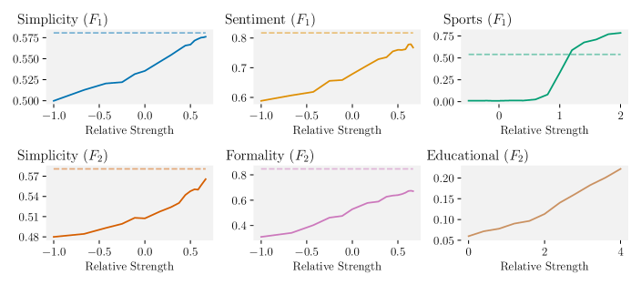
Figure 2: Attribute presence for several attributes and formulas. Dashed line indicates the value of the attribute when prompting the model to use the attribute.

We depict results in Fig. 2 where the $x$-axis shows the value of $\lambda_{i}$ normalized by the sum of all $\lambda$ coefficients occurring in the resulting optimization problem and the $y$-axis shows attribute strength according to popular classifiers from the HuggingFace library (Wolf et al., 2020). The presence of an attribute indeed increases smoothly as the associated $\lambda_{i}$ increases. Interestingly, the curves, except for the sports attribute, suggest a linear relationship, indicating that the presence of the attribute increases predictably with the relative strength. This aligns with our interpretation of model arithmetic as (linear) operators in logit space. Further, these results show the intuitive semantics of model arithmetic extends to the characteristics of the generated output on a sequence level. Because of its formulation with a counterweight, the curve associated with $\lambda_{3}$ and the sports attribute shows very different behavior. Indeed, the sports attribute only gets a significant boost once its relative strengths passes $1.0$. At this point the $(1-\lambda_{3})$ coefficient, counterweighing $\bm{{M_{\text{helpful}}}}$, biases away from any behavior that is not associated with $\operatorname{union}(\bm{{M_{\text{helpful}}}},\bm{{M_{\text{sports}}}})$, emphasizing this term more than what would be possible under regular prompting. At this point, the presence of the sports attribute increases even beyond the indicated value achieved by standard prompting (cf. Fig. 2, top right).

Finally, we note that this fine-grained control comes at very little cost with respect to perplexity. The highest perplexity across all formulas and attributes is $6.2$, which is only slightly higher than the highest perplexity of the 5 prompted models, namely $4.8$. In Section H.2 we show in more detail that the fluency of the generated text is not affected by the use of model arithmetic, except for the educational attribute at the highest evaluated strengths where fluency is slightly affected due to the heavy use of a (fluency-agnostic) classifier.

5.3 Speculative Sampling

Table 7: Evaluation of Llama-2-13b-Chat with speculative sampling where $F_{1}=0.2\bm{{M_{\text{formal}}}}+0.5\bm{{M_{\text{happy}}}}+0.05\bm{{M_{\text{sports}}}}$ and $F_{2}=\bm{{M_{\text{formal}}}}+0.1\bm{{M_{\text{angry}}}}+0.4\bm{{M_{\text{sports}}}}$.

$\operatorname{supersede}(\bm{{A}},\bm{{M}})$	Calls per Token		Time per Token [ms]
	No Spec.	Spec.	No Spec.	Spec.
	$1$	$0.801\,487\,144\,577\,682\,3$	$24.883\,752\,406\,564\,422$	$22.801\,977\,472\,271\,506$
$+0.5\bm{{M_{\text{formal}}}}$	$2.0$	$1.034\,879\,464\,519\,165\,5$	$48.402\,358\,490\,574\,5$	$30.432\,601\,378\,073\,695$
$+0.5\bm{{M_{\text{happy}}}}$	$2.0$	$1.044\,895\,168\,641\,750\,2$	$49.150\,893\,497\,867\,39$	$31.190\,228\,983\,827\,797$
$+0.5\bm{{M_{\text{sports}}}}$	$2.0$	$1.075\,711\,031\,340\,604\,6$	$49.262\,453\,864\,134\,244$	$31.999\,939\,596\,160\,875$
$+0.5\bm{{M_{\text{easy}}}}$	$2.0$	$1.100\,019\,891\,860\,612\,3$	$49.201\,301\,989\,288\,18$	$32.749\,359\,688\,622\,356$
$+0.5\bm{{M_{\text{angry}}}}$	$2.0$	$1.119\,715\,506\,947\,929\,4$	$49.286\,456\,629\,735\,51$	$33.011\,800\,235\,675\,22$
$+F_{1}$	$4.0$	$1.316\,517\,137\,450\,059\,5$	$97.025\,533\,724\,569\,8$	$43.259\,894\,817\,789\,73$
$+F_{2}$	$4.0$	$1.435\,912\,927\,894\,491\,5$	$97.019\,219\,898\,991\,65$	$46.100\,464\,548\,583\,346$

Next, we show the effect of speculative sampling on the evaluation of model arithmetic expressions. We use the same setup as in Section 5.2 with the only difference that we optimize the speculative factors $s_{i}$ based on a single calibration run of 10 samples with a procedure detailed in Section E.1. To evaluate the effect of the $\operatorname{supersede}$ operation in model arithmetic, we use an autocompletion model $A$, which statically predicts the most likely next token based on the previous and fitted on the Alpaca dataset (Taori et al., 2023).

Figure 3: Model calls per token with speculative sampling for $\bm{{M}}+\lambda\bm{{M_{a}}}$, $\lambda\in[0.1,1.0]$.

In Table 7 we show that speculative sampling significantly reduces the number of model calls and increases inference speed. Just $\operatorname{supersede}(\bm{{A}},\bm{{M}})$ reduces the number of model calls by 20% compared to $\bm{{M}}$. Applying speculative sampling to larger formulas, we can reduce the number of model calls to at most $1.44$ per token, even in the presence of up to 4 constituent models, where this leads to a boost in inference speed by up $2.24$ times.

Further, for $F:=\bm{{M}}+\lambda\bm{{M_{a}}}$, Fig. 3 shows that the number model calls per token increases with $\lambda$. The reason for this is that as $\lambda$ increases the KL-divergence between the original model $\bm{{M}}$ and the distribution described by $F$ increases, which in turn decreases acceptance probability in speculative sampling.

6 Related Work

We now briefly review related approaches related to model arithmetic.

Controlled Text Generation

Several works have interpreted CTG from perspectives differing from Bayes rule, either through the minimization of the model loss under various hard constraints (Meng et al., 2022; Kumar et al., 2021; 2022), by modifying the model output based on the gradients of a classifier model (Dathathri et al., 2020), or by reducing the mutual information between the output and the attribute (Yang et al., 2023). However, all these works either require costly gradient steps during the decoding phase or demand training data for the model. We have discussed CTG without relying on any training data or expensive gradient steps in Section 2 and compare to them in Section 5.1.

Speculative Sampling

Recent work extend on speculative sampling to use multiple smaller models in a staged fashion (Spector and Re, 2023) or by using multiple small models at once (Miao et al., 2023). Moreover, both methods use a tree-based sampling approach to generate multiple proposal sequences of the smaller models at once. We note that these improvements can be incorporated orthogonally in our extension of speculative sampling as the $\operatorname{supersede}$ operator.

7 Conclusion

We introduced model arithmetic, a novel framework for composing multiple LLMs and controlled generation attributes, using a principled formula-based approach. Our method offers precise control over model output and can be used to express many prior controlled text generation (CTG) techniques. By leveraging this expressiveness and a novel model $\operatorname{union}$ operator, model arithmetic subsumes prior approaches for CTG-based toxicity reduction and significantly outperforms them. Further, we derived a speculative sampling procedure for model arithmetic formulas, allowing us to heavily reduce the computational overhead typically associated with multi-model CTG.

Broader Impact

While model arithmetic provides additional flexibility and expressiveness, we note that it can also be used to generate text containing undesirable attributes. For example, instead of reducing toxic content, one could use model arithmetic to increase toxic content, potentially even avoiding build-in safety filters (Touvron et al., 2023; OpenAI, 2023). While this is a problem that is not unique to model arithmetic, it is more important due to the increased control and complexity of the formulas. However, we believe the benefits of model arithmetic outweigh the potential risks, as it allows for more precise control and expressiveness, which can be used to generate more inclusive and controlled content.

Reproducibility

We provide code along with instructions for all experiments with the submission and provide all required experimental details in App. G.

Appendix A Prior Work

Table 8: Previous work that can be expressed using our framework. $U$ denotes the uniform distribution, $C$ is a classifier, $a,a_{1},a_{2}$ are textual descriptions of attributes and $M_{a}$ is the language model $M$ prompted with this additional textual description. $\operatorname{TopK}$ denotes that top-k sampling is required for efficiency due to the used classifier $C$, while else the choice of sampling techniques is not restricted.

Citation	Formula	Sampling	Training method
Liu et al. [2021]	$\bm{{M}}+\lambda(\bm{{m_{p}}}-\bm{{m_{n}}})$	-	$m_{p}$ (resp. $m_{n}$) is a small model fine-tuned on positive (resp. negative) samples.
Pei et al. [2023]	$\bm{{M}}+\lambda\bm{{M_{a}}}$	-	No training applied.
Sanchez et al. [2023]	$\bm{{M}}+\lambda\bm{{M_{a}}}$	-	No training applied.
Chen et al. [2022]	$\bm{{M}}+\lambda_{1}\bm{{M_{a_{1}}}}-\lambda_{2}\bm{{M_{a_{2}}}}$	-	No training applied.
Yang and Klein [2021]	$\bm{{M}}+\bm{{C}}$	$\operatorname{TopK}$	The classifier is trained on partial samples.
Kim et al. [2023]	$\bm{{M}}+\bm{{C}}$	$\operatorname{TopK}$	The classifier is trained using Reinforcement Learning.
Meng et al. [2022]	$\bm{{M}}+\bm{{C}}$	-	The trained classifier outputs a probability for each token at the same time.
Sitdikov et al. [2022]	$\bm{{M}}+\lambda\bm{{C}}$	$\operatorname{TopK}$	No training applied.

Table 8 shows how multiple prior works can be expressed in model arithmetic.

Appendix B Intersection

The optimization problem obtained by switching the indicator functions for the $\operatorname{union}$ is equal to

$$D_{\mathrm{KL}}^{[\mathcal{I}_{2}]}(P||Q_{1})+D_{\mathrm{KL}}^{[\mathcal{I}_{1}]}(P||Q_{2}).$$

The solution to this problem is equal to $\sigma(\min(\log Q_{1},\log Q_{2}))$. We define the $\operatorname{intersection}$ operator as this solution and note that it assigns a high probability to a specific token, only if both $Q_{1}$ and $Q_{2}$ have a high probability associated with it.

Appendix C Attribution

The icons in Fig. 1 are from flaticon.com: $M_{\text{child}}$, $M_{\text{adult}}$, $M_{\text{magic}}$, $C_{\text{formal}}$ all by Freepik.

Appendix D Proofs

D.1 Solution Minimization Problem

We present the proof and assumptions of Theorem 1 here.

Assumptions

We first introduce the assumptions that we make in order to prove Theorem 1. We assume that for any $k\in\{1,...,t\}$, $\sum_{i=1}^{n}f_{i}(x,x_{1:k-1})$ is independent of $x$ for all $x\in T$ and

$$\sum_{i=1}^{n}f_{i}(x,x_{1:k-1})>0.$$

The first assumption is necessary for proper normalization of the output distribution. Even though it looks like a very stringent assumption, it is in fact quite mild. Indeed, if a formula $\sum_{i}\bm{{f_{i}}}\bm{{Q_{i}}}$ does not satisfy the assumption, then we can simply replace $\bm{{f_{1}}}$ with $\bm{{f_{1}^{\prime}}}=\bm{{f_{1}}}-\sum_{i=2}^{n}\bm{{f_{i}}}$. This essentially changes the influence of $Q_{1}$ to be appropriately scaled for different tokens. The second assumption is necessary to ensure that the optimization problem is meaningful. Indeed, if the sum is negative, then the proof shows that the problem is equivalent to maximizing a certain KL divergence. Maximizing a KL divergence without any other constraints gives no meaningful notion in practice.

We now prove Theorem 1.

Proof.

We first define

$$G(P,x_{1:k-1})=\sum_{i=1}^{n}D_{\mathrm{KL}}^{[f_{i}]}(P||Q_{i}|x_{1:k-1})$$

and thus the problem can be written as $\operatorname*{arg\,min}_{P}G(P,x_{1:k-1})$. In order to prove the theorem, we expand the KL-divergence in $G$ and use logarithmic properties to obtain

$$G(P,x_{1:k-1})=\sum_{i=1}^{n}\sum_{x\in T}P(x|x_{1:k-1})\log\left(\frac{P(x|x_{1:k-1})}{Q_{i}(x|x_{1:k-1})}\right)^{f_{i}(x,x_{1:k-1})}.$$

We then swap the summations and write the second sum in the logarithm as a product

$$G(P,x_{1:k-1})=\sum_{x\in T}P(x|x_{-k})\log\prod_{i=1}^{n}\left(\frac{P(x|x_{1:k-1})}{Q_{i}(x|x_{1:k-1})}\right)^{f_{i}(x,x_{1:k-1})}.$$

We now introduce the notation $f_{S}(x_{1:k-1}):=\sum_{i=1}^{n}f_{i}(x,x_{1:k-1})$, where we use the assumption that $\sum_{i=1}^{n}\ f_{i}(x,x_{1:k-1})$ is independent of $x$, and rewrite to get

$$G(P,x_{1:k-1})=f_{S}(x_{1:k-1})\sum_{x\in T}P(x|x_{1:k-1})\log\left(\frac{P(x|x_{1:k-1})}{\prod_{i=1}^{n}Q_{i}(x|x_{1:k-1})^{\frac{f_{i}(x,x_{1:k-1})}{f_{S}(x_{1:k-1})}}}\right).$$

We now note that the right term of $G(P,x_{1:k-1})$ is again a KL-divergence up to some constants in the denominator of the logarithm. Since by assumption $f_{S}(x_{1:k-1})>0$ and since $D_{\mathrm{KL}}(P||Q)$ is minimized for $P=Q$, we get

$$\log P(x_{k}=x|x_{1:k-1})\propto\frac{1}{f_{S}(x_{1:k-1})}\sum_{i=1}^{n}f_{i}(x,x_{1:k-1})\log Q_{i}(x|x_{1:k-1}).$$

Introducing the correct constants, we get the desired result

$$\log P(x_{k}|x_{-k})=\log\sigma\left(\frac{1}{\sum_{i=1}^{n}f_{i}(x,x_{1:k-1})}\sum_{i=1}^{n}f_{i}(x,x_{1:k-1})\log Q_{i}(x_{k}|x_{-k})\right)$$

∎

D.2 Classifier Formula

We prove the following lemma.

Lemma 2.

Let $T$ be the set of all tokens and let $x_{1:k-1}$ be a given sequence of tokens. Let $C:T^{k}\rightarrow[0,1]$ be a binary classifier and $U$ the uniform distribution over $T$. Let $Q_{C}$ be the distribution defined by $Q_{C}(x|x_{1:k-1})\propto C(x,x_{1:k-1})$ for all $x\in T$. Then

$$\operatorname*{arg\,min}_{P}-\sum_{x\in T}P(x|x_{1:k-1})\log C(x_{1:k-1},x)=\operatorname*{arg\,min}_{P}D_{\mathrm{KL}}(P||Q_{C})-D_{\mathrm{KL}}(P||U)$$

Proof.

We prove the following equality

$$-\sum_{x\in T}P(x|x_{1:k-1})\log C(x_{1:k-1},x)=D_{\mathrm{KL}}(P||Q_{C})-D_{\mathrm{KL}}(P||U)+\mathcal{C}$$ (4)

where $\mathcal{C}\in\mathbb{R}$ is a constant. Since a constant has no influence on the optimization problem, the required equivalence holds.

We now drop $x_{1:k-1}$ for readability. We then expand the right term of Eq. 4 using the definition of the KL-divergence to get

$$D_{\mathrm{KL}}(P||Q_{C})-D_{\mathrm{KL}}(P||U)=\sum_{x\in T}P(x)\log\frac{P(x)}{Q_{C}(x)}-\sum_{x\in T}P(x)\log\frac{P(x)}{U(x)}.$$

Making use of logarithmic properties, we rewrite and simplify to get

$$D_{\mathrm{KL}}(P||Q_{C})-D_{\mathrm{KL}}(P||U)=\sum_{x\in T}-P(x)\log Q_{C}(x)+\sum_{x\in T}P(x)\log U(x).$$

We now note that the second term is a constant (equal to $\log(1/|T|)$) and we use the definition of $Q_{C}$ to rewrite the first term to

$$\sum_{x\in T}-P(x)\log Q_{C}(x)=-\sum_{x\in T}P(x)\log C(x)+\sum_{x\in T}P(x)\log\left(\sum_{y\in T}C(y)\right).$$

The second term is again a constant and since the first term is the expected cross-entropy, we get the desired result. ∎

D.3 Speculative Sampling on N Distributions

We prove Lemma 1 here.

Proof.

The proof follows an induction algorithm. For $n=2$ the lemma follows from a direct application of speculative sampling [Chen et al., 2023]. We assume that the theorem holds for $n$ distributions and show that it also holds for $n+1$ distributions. We first apply the procedure to $(P_{1},P_{2}),\ldots,(P_{n-1},P_{n})$ which by induction gives us a sample $x^{\prime}\sim P_{n}$. We then apply the procedure to $(P_{n},P_{n+1})$ which gives us a sample $x^{\prime\prime}\sim P_{n+1}$, also by induction. Therefore, we have a sample $x^{\prime\prime}$ sampled from $P_{n+1}$ which proves the lemma. ∎

Appendix E Speculative Algorithm for Model Arithmetic

Algorithm 1 shows the standard speculative sampling method. When using it with a small model $m$ and a large model $M$, we simply set $P_{1}=m$ and $P_{2}=M$ and run the algorithm as specified.

Algorithm 2 shows the detailed procedure for applying speculative sampling to model arithmetic. We first initialize the variables keeping track of the number of tokens that have been generated by each model and the prediction history of all models in 2–3. We then start generating tokens and in 6 we check if the current model under consideration needs to be run. If so, we run the standard speculative sampling method in 11–23 on the distributions with and without the model. We then continue generating tokens until we have generated $N$ tokens.

Algorithm 1 $\mathrm{SpeculativeSampling}(P_{1},P_{2},x_{1:k-1},x_{k})$

1:generating distribution $P_{1}$, validating distribution $P_{2}$, sequence $x_{1:k-1}$ and proposed token $x_{k}\sim P_{1}(x|x_{1:k-1})$.

2:$a=\min\left(1,\frac{P_{2}(x_{k}|x_{1:k-1})}{P_{1}(x_{k}|x_{1:k-1})}\right)$

3:$r\sim\mathrm{Uniform}(0,1)$

4:if $r<a$ then

5:     return $x_{k}$

6:else

7:     $P_{2}^{\prime}(x|x_{1:k-1})=\frac{\max(P_{2}(x|x_{1:k-1})-P_{1}(x|x_{1:k-1}),0)}{\sum_{y\in T}\max(P_{2}(x|x_{1:k-1})-P_{1}(x|x_{1:k-1}),0)}$

8:     return $\mathrm{sample}(P_{2}^{\prime}(x|x_{1:k-1}))$

9:end if

Algorithm 2 Speculative Sampling on $n$ distributions

1:Formula $F=\sum_{i=1}^{n}\lambda_{i}\bm{{f_{i}^{\prime}}}\bm{{Q_{i}}}$, speculative factors $s_{1},\ldots,s_{n}$, input tokens $X=x_{1},\ldots,x_{k}$, number of tokens to generate $N$, token space $T$.

2:$\text{tokens}=\text{zeros}(\text{shape}=(n,))$

3:$H=\text{zeros}(\text{shape}=(n,N,|T|))$

4:while $\text{len}(X)<N$ do

5:     for $i$ in $1,\ldots,n$ do

6:         if $\text{tokens}_{i}<s_{i}$ then

7:              $\text{tokens}_{j}=\text{tokens}_{j}+1$

8:         else

9:              $\text{tokens}_{j}=0$

10:              $H_{i,\text{len}(X)-s_{i}:\text{len}(X)+1}$ = Run $\lambda_{i}\bm{{f_{i}^{\prime}}}\bm{{Q_{i}}}$ and return output for the new $s_{i}+1$ tokens.

11:              for $j$ in $\text{len}(X)-s_{i},\ldots,\text{len}(X)$ do

12:                  $P_{\text{old}}=-H_{i,j}+\sum_{l=1}^{n}H_{l,j}$

13:                  $P_{\text{new}}=\sum_{l=1}^{n}H_{l,j}$

14:                  $X_{j}^{\prime}=\mathrm{SpeculativeSampling}(P_{\text{old}},P_{\text{new}},X_{1:j-1},X_{j})$

15:                  if $X_{j}^{\prime}\neq X_{j}$ then

16:                       $X=[X_{1:j-1},X_{j}^{\prime}]$

17:                       $H=H_{:,:j+1}$

18:                       break

19:                  end if

20:              end for

21:              if $j=\text{len}(X)$ then

22:                  $X=[X,\mathrm{sample}(\sum_{l=1}^{n}H_{l,j})]$

23:              end if

24:         end if

25:     end for

26:end while

27:return $X$

E.1 Determining Speculative Factors

Here, we explain our approach for selecting the speculative factors in more detail. We first show that the probability that a token $x\sim P_{1}$ is accepted by $P_{2}$ is equal to $1-\frac{1}{2}\sum_{x}|P_{1}(x)-P_{2}(x)|$.

Lemma 3.

Given two discrete distributions $P_{1}$ and $P_{2}$. The procedure described in Algorithm 1 returns the same token as its input $x\sim P_{1}$ with a probability that is in expectation equal to $1-\frac{1}{2}\sum_{x}|P_{1}(x)-P_{2}(x)|$.

Proof.

We call the probability that the input token $x$ is returned $a(x_{k})$ and refer to it as the acceptance probability. We then find that the expected acceptance probability is

$$\mathbb{E}_{x\sim P_{1}}(a(x))=\sum_{x}P_{1}(x)\min\left(1,\frac{P_{2}(x)}{P_{1}(x)}\right)=\sum_{x}\min(P_{2}(x),P_{1}(x))$$

Rewriting this by making use of $\sum_{x}P_{2}(x)=\sum_{x}P_{1}(x)=1$ gives

$$\mathbb{E}_{x\sim P_{1}}(a(x))=1+\sum_{x}\min(P_{2}(x),P_{1}(x))-\frac{1}{2}P_{1}(x)-\frac{1}{2}P_{2}(x).$$

Again rewriting leads us to

$$\mathbb{E}_{x\sim P_{1}}(a(x)) =1+\sum_{x}\frac{1}{2}\min(P_{2}(x)-P_{1}(x),0)+\frac{1}{2}\min(P_{1}(x)-P_{2}(x),0)$$

$$=1-\frac{1}{2}\sum_{x}|P_{1}(x)-P_{2}(x)|.$$

which gives us the desired result. ∎

We now explain our approach for selecting the speculative factors. We first assume that the evaluation of the formula only consist of two terms, $\lambda_{1}\bm{{f_{1}^{\prime}}}\bm{{Q_{1}}}+\lambda_{2}\bm{{f_{2}^{\prime}}}\bm{{Q_{2}}}$. Since one model needs to be evaluated every time (otherwise one would generate tokens from the uniform distribution), we set $s_{1}=1$ and find a simplified procedure to optimize the speculative factor $s_{2}$. Suppose $C_{1}$ (resp. $C_{2}$) is the amount of compute required to calculate $\lambda_{1}\bm{{f_{1}^{\prime}}}\bm{{Q_{1}}}$ (resp. $\lambda_{2}\bm{{f_{2}^{\prime}}}\bm{{Q_{2}}}$). Let the expected probability that a token proposed by $\lambda_{1}\bm{{f_{1}^{\prime}}}\bm{{Q_{1}}}$ is accepted be $a$. We determine this acceptance probability by using Lemma 3 and averaging it over a small corpus of 10 samples.

Every time we compute $\lambda_{2}\bm{{f_{2}^{\prime}}}\bm{{Q_{2}}}$, we compute $\lambda_{1}\bm{{f_{1}^{\prime}}}\bm{{Q_{1}}}$ exactly $s_{2}$ times. Therefore the amount of compute spent for a single large computation is $C_{2}+s_{2}C_{1}$. The expected amount of accepted tokens after this is equal to $1+a+\ldots+a^{s_{2}-1}$. Therefore, the expected amount of compute spent per token is

$$C_{\text{per token}}(s_{1},s_{2},C_{1},C_{2})=\frac{C_{2}+s_{2}C_{1}}{1+a+\ldots+a^{s_{2}-1}}=(1-a)\frac{C_{2}+s_{2}C_{1}}{1-a^{s_{2}}}.$$

We note that the second derivative of $C_{\text{per token}}$ with respect to $s_{2}$ is negative everywhere and therefore the minimization problem

$$\operatorname*{arg\,min}_{s_{2}}C_{\text{per token}}(s_{1},s_{2},C_{1},C_{2})$$

is convex. The optimal $s_{2}$ can thus be determined by using standard optimization techniques.

We generalize this approach to $n$ terms simply by assuming that the expected acceptance probability for the term $\lambda_{i}\bm{{f_{i}^{\prime}}}\bm{{Q_{i}}}$ is constant no matter how many models have been run before. By doing so, we can follow the exact same approach as before to determine the optimal speculative factors for all terms, where we consider $\lambda_{1}\bm{{f_{1}^{\prime}}}\bm{{Q_{1}}}$ to be a single model call and $\lambda_{2}\bm{{f_{2}^{\prime}}}\bm{{Q_{2}}}$ the current model $\lambda_{i}\bm{{f_{i}^{\prime}}}\bm{{Q_{i}}}$.

Table 9: Sentiment and perplexity of various methods on the IMDB movie dataset with negative reviews. $\bm{{M}}$, $\bm{{M_{\text{pos}}}}$ and $\bm{{M_{\text{neg}}}}$ denote the model without conditioning, conditioning to positive sentiment and conditioning to negative sentiment respectively. $\bm{{C}}$ is a sentiment classifier. Perplexity is measured with respect to $\bm{{M}}$. For perplexity lower is better, for sentiment higher is better.

	Llama-2-13b		Pythia-12b		MPT-7b
	Sent.	Perpl.	Sent.	Perpl.	Sent.	Perpl.
$\bm{{M}}$	$0.201\,135\,894\,775\,390\,62$	$13.128\,526\,202\,684\,414$	$0.209\,830\,474\,853\,515\,64$	$24.101\,486\,545\,536\,73$	$0.204\,386\,352\,539\,062\,5$	$19.916\,645\,213\,602\,056$
$\bm{{M_{\text{pos}}}}$	$0.264\,026\,275\,634\,765\,6$	$12.444\,268\,241\,432\,498$	$0.220\,720\,703\,125$	$22.679\,810\,492\,141\,94$	$0.226\,884\,643\,554\,687\,5$	$18.413\,235\,121\,581\,188$
SelfDebias ($\lambda=10$)	$0.256\,628\,753\,662\,109\,35$	$13.606\,173\,061\,550\,008$	$0.255\,499\,908\,447\,265\,6$	$26.317\,207\,377\,452\,345$	$0.234\,638\,793\,945\,312\,5$	$20.307\,906\,178\,929\,42$
Fudge ($\bm{{M_{\text{pos}}}}+\bm{{C}}$)	$0.327\,788\,543\,701\,171\,9$	$13.005\,064\,175\,684\,339$	$0.308\,287\,963\,867\,187\,5$	$24.033\,395\,450\,821\,555$	$0.314\,036\,895\,751\,953\,15$	$19.853\,348\,344\,205\,916$
PreAdd ($\bm{{M_{\text{pos}}}}-0.6\bm{{M_{\text{neg}}}}$)	$0.398\,091\,400\,146\,484\,36$	$12.944\,179\,954\,661\,738$	$0.353\,229\,980\,468\,75$	$30.280\,386\,996\,263\,1$	$0.321\,626\,861\,572\,265\,6$	$19.559\,241\,394\,254\,045$
$\bm{{M_{\text{pos}}}}-0.96\cdot\operatorname{union}(\bm{{M_{\text{neg}}}},\bm{{M_{\text{pos}}}})$	$0.393\,317\,565\,917\,968\,74$	$10.170\,443\,906\,469\,423$	$0.337\,419\,097\,900\,390\,65$	$22.859\,155\,526\,820\,643$	$0.375\,122\,406\,005\,859\,4$	$18.474\,184\,303\,715\,21$
$\bm{{M_{\text{pos}}}}-0.96\cdot\operatorname{union}(\bm{{M_{\text{neg}}}},\bm{{M_{\text{pos}}}})+0.04\bm{{C}}$	$0.466\,283\,111\,572\,265\,65$	$10.398\,901\,188\,444\,746$	$0.416\,063\,323\,974\,609\,4$	$24.880\,639\,272\,000\,07$	$0.452\,088\,745\,117\,187\,5$	$19.067\,004\,889\,981\,032$

Table 10: Comparison of our method with PreAdd and Fudge using GPT-4 for the positive sentiment task. Ours ($\operatorname{union}$) is the formula $\bm{{M_{\text{pos}}}}-0.96\cdot\operatorname{union}(\bm{{M_{\text{neg}}}},\bm{{M_{\text{pos}}}})$ and Ours (Combined) is the formula $\bm{{M_{\text{pos}}}}-0.96\cdot\operatorname{union}(\bm{{M_{\text{neg}}}},\bm{{M_{\text{pos}}}})+0.04\bm{{C}}$. Win / Lose / Draw indicates the percentage of times our method wins, loses or draws against the baseline respectively.

		Llama-2-13b	Pythia-12b	MPT-7b
	Baseline	Win / Lose / Draw	Win / Lose / Draw	Win / Lose / Draw
Ours ($\operatorname{union}$)	Fudge	$\mathbb{0.45}/0.29/0.26$	$\mathbb{0.36}/0.32/0.32$	$\mathbb{0.44}/0.26/0.30$
	PreAdd	$\mathbb{0.41}/0.35/0.24$	$\mathbb{0.38}/0.32/0.31$	$\mathbb{0.39}/0.29/0.31$
Ours (Combined)	Fudge	$\mathbb{0.51}/0.24/0.24$	$\mathbb{0.43}/0.29/0.28$	$\mathbb{0.52}/0.22/0.26$
	PreAdd	$\mathbb{0.47}/0.32/0.21$	$\mathbb{0.44}/0.31/0.25$	$\mathbb{0.46}/0.29/0.25$

Appendix F Sentiment Control

We evaluate model arithmetic on the task of sentiment control and closely follow the setup described in Pei et al. [2023]. For this purpose, we select 1000 positive and 1000 negative reviews from the IMDB movie review dataset [Maas et al., 2011]. For each model, we stop the review at 32 tokens. The goal is to continue the review in a sentiment opposite to the original movie review. Further experimental details are shown in Section G.2. We used the same hyperparameters for the models as for the toxicity reduction task.

Results are presented for the tasks of converting negative reviews to positive reviews in Table 9 and converting positive reviews to negative reviews in Table 11. Furthermore, GPT-4 is prompted to select the best response in terms of sentiment and relevance for the positive sentiment task in Table 10 and for the negative sentiment task in Table 12.

We find that our $\operatorname{union}$ operator still significantly outperforms all baselines, especially when evaluating the results with GPT-4. GPT-4 prefers our method for all evaluated settings over the baselines and that with an average of 5% over the closest following baseline, PreAdd. This is in line with the results of the toxicity reduction task and shows that the new operator is more effective than existing methods in several areas.

Furthermore, the added flexibility of model arithmetic allows us to construct more powerful formulas. As in the toxicity task, combining the $\operatorname{union}$ operator with a classifier outperforms all other methods by a wide margin. In fact, GPT-4 prefers this formula over PreAdd for all cases with a 12% difference in preference on average. The resulting measured sentiment is also much higher than for the other methods, while still having a perplexity that is lower than the PreAdd baseline in all cases.

Table 11: Sentiment and perplexity of various methods on the IMDB movie dataset with positive reviews. $\bm{{M}}$, $\bm{{M_{\text{pos}}}}$ and $\bm{{M_{\text{neg}}}}$ denote the model without conditioning, conditioning to positive sentiment and conditioning to negative sentiment respectively. $\bm{{C}}$ is a sentiment classifier. Perplexity is measured with respect to $\bm{{M}}$. Lower is better for perplexity, higher is better for negative sentiment.

	Llama-2-13b		Pythia-12b		MPT-7b
	Neg. Sent.	Perpl.	Neg. Sent.	Perpl.	Neg. Sent.	Perpl.
$\bm{{M}}$	$0.196\,082\,244\,873\,046\,87$	$12.047\,795\,387\,544\,605$	$0.209\,830\,734\,252\,929\,7$	$22.332\,962\,213\,647\,157$	$0.193\,059\,745\,788\,574\,2$	$17.778\,516\,857\,408\,835$
$\bm{{M_{\text{neg}}}}$	$0.282\,465\,301\,513\,671\,9$	$12.619\,133\,853\,486\,643$	$0.322\,156\,669\,616\,699\,2$	$23.204\,974\,562\,510\,8$	$0.255\,451\,660\,156\,25$	$18.636\,694\,999\,757\,555$
SelfDebias ($\lambda=10$)	$0.311\,862\,533\,569\,335\,96$	$14.304\,233\,675\,729\,689$	$0.363\,237\,747\,192\,382\,83$	$26.416\,303\,631\,864\,015$	$0.277\,779\,449\,462\,890\,6$	$20.227\,345\,851\,977\,553$
Fudge ($\bm{{M_{\text{neg}}}}+\bm{{C}}$)	$0.379\,331\,047\,058\,105\,44$	$12.749\,501\,165\,767\,288$	$0.420\,116\,149\,902\,343\,75$	$23.648\,448\,919\,299\,245$	$0.359\,748\,046\,875$	$18.516\,850\,214\,336\,41$
PreAdd ($\bm{{M_{\text{neg}}}}-0.6\bm{{M_{\text{pos}}}}$)	$0.453\,678\,115\,844\,726\,56$	$13.968\,328\,400\,468\,21$	$0.506\,502\,746\,582\,031\,2$	$32.931\,431\,549\,580\,41$	$0.420\,524\,307\,250\,976\,56$	$19.927\,424\,932\,649\,348$
$\bm{{M_{\text{neg}}}}-0.96\cdot\operatorname{union}(\bm{{M_{\text{neg}}}},\bm{{M_{\text{pos}}}})$	$0.469\,199\,539\,184\,570\,3$	$13.154\,075\,914\,961\,544$	$0.470\,654\,479\,980\,468\,8$	$26.226\,811\,574\,924\,263$	$0.421\,869\,613\,647\,460\,95$	$18.352\,602\,515\,877\,41$
$\bm{{M_{\text{neg}}}}-0.96\cdot\operatorname{union}(\bm{{M_{\text{neg}}}},\bm{{M_{\text{pos}}}})+0.04\bm{{C}}$	$0.523\,920\,120\,239\,257\,8$	$13.307\,529\,161\,162\,595$	$0.544\,454\,002\,380\,371\,1$	$27.468\,739\,087\,468\,098$	$0.509\,180\,419\,921\,875$	$18.560\,302\,136\,466\,998$

Table 12: Comparison of our method with PreAdd and Fudge using GPT-4 for the positive sentiment task. Ours ($\operatorname{union}$) is the formula $\bm{{M_{\text{neg}}}}-0.96\cdot\operatorname{union}(\bm{{M_{\text{neg}}}},\bm{{M_{\text{pos}}}})$ and Ours (Combined) is the formula $\bm{{M_{\text{neg}}}}-0.96\cdot\operatorname{union}(\bm{{M_{\text{neg}}}},\bm{{M_{\text{pos}}}})+0.04\bm{{C}}$. Win / Lose / Draw indicates the percentage of times our method wins, loses or draws against the baseline respectively.

		Llama-2-13b	Pythia-12b	MPT-7b
	Baseline	Win / Lose / Draw	Win / Lose / Draw	Win / Lose / Draw
Ours ($\operatorname{union}$)	Fudge	$\mathbb{0.51}/0.34/0.15$	$\mathbb{0.47}/0.36/0.17$	$\mathbb{0.47}/0.35/0.18$
	PreAdd	$\mathbb{0.45}/0.42/0.12$	$\mathbb{0.45}/0.44/0.12$	$\mathbb{0.43}/0.40/0.17$
Ours (Combined)	Fudge	$\mathbb{0.54}/0.32/0.14$	$\mathbb{0.52}/0.34/0.14$	$\mathbb{0.51}/0.28/0.21$
	PreAdd	$\mathbb{0.47}/0.42/0.12$	$\mathbb{0.50}/0.40/0.10$	$\mathbb{0.48}/0.37/0.15$

Appendix G Experimental Details

All our experiments were run on a single H100 Nvidia GPU with 80GB of VRAM.

G.1 Training and Prompting Details Toxicity Reduction

We present the prompting details for the toxicity reduction in Section 5.1 here. We use Llama-2-13b [Touvron et al., 2023], Pythia-12b [Biderman et al., 2023] and MPT-7b [Team, 2023] as the models for evaluation.

We finetune a classifier for Fudge by starting from a RoBERTa based [Liu et al., 2019] toxicity classifier and finetuning it for 5 epochs with a learning rate of 1e-5 on the Jigsaw toxicity dataset [cjadams et al., 2017] using the method described in Yang and Klein [2021]. The Jigsaw dataset was preprocessed to contain the same amount of toxic as non-toxic sentences.

Before selecting the input messages from the /pol/ dataset Papasavva et al. [2020], we first filter messages that contain links and html. We then select 2000 random messages with a toxicity score higher than 0.5. Each message is then prompted as if it came out of a conversation by using the template

Person 1:{{MESSAGE}}
Person 2:{{COMPLETION}}

and completions are stopped when they reach more than 32 tokens, contain the newline token, the end of sequence token or the sequence ‘Person 1:’.

Additionally, we prepend a non-toxic (resp. toxic) sentence to the prompt for $M_{\text{non-toxic}}$ (resp. $M_{\text{toxic}}$) to bias generations towards a non-toxic (resp. toxic) completion. The prompts used are inspired by [Pei et al., 2023]. Specifically, the non-toxic sentence is

The following conversation is one that does not perpetuate negative stereotypes, is not threatening and does not contain any sexually explicit or profane language.

and the toxic sentence is

The following conversation is one that perpetuates negative stereotypes, is threatening or sexually explicit and contains profane language.

G.2 Training and Prompting Details Sentiment Control

We present the prompting details for the sentiment control task presented in App. F here. We use Llama-2-13b [Touvron et al., 2023], Pythia-12b [Biderman et al., 2023] and MPT-7b [Team, 2023] as the models for evaluation.

We finetune a classifier for Fudge by starting from the RoBERTA base model [Liu et al., 2019] and finetuning it for 5 epochs with a learning rate of 1e-5 on the IMDB dataset [Maas et al., 2011] using the method described in Yang and Klein [2021]. We compute the sentiment scores using a popular sentiment classifier fine-tuned from the RoBERTa base model [Camacho-collados et al., 2022].

We then randomly select 1000 positive and 1000 negative movie reviews from the IMDB dataset [Maas et al., 2011]. For each model, we stop the input review after 32 tokens and use these as input messages. The model $M$ solely receives the input message as prompt, while the models $M_{\text{pos}}$ and $M_{\text{neg}}$ receive the input message with a simple sentence prepended to it to continue the review in a positive and negative fashion respectively. The positive sentence is

The following is a positive movie review, with a very positive sentiment and a very positive tone.

and the negative sentence is

The following is a negative movie review, with a very negative sentiment and a very negative tone.

Finally, a continuation is stopped when it reaches more than 64 tokens or contains the newline or the end of sequence token.

G.3 GPT-4 Prompting Details

We used GPT-4 [OpenAI, 2023] to evaluate the outputs of several methods and obtain its preference between them for both the toxicity reduction task and sentiment control task.

For the toxicity task, we constructed a prompt that asks GPT-4 to select the better completion between two methods. GPT-4 is given the input message along with the completions of two methods and asked to select the better completion, or to select neither if it cannot decide.

Specifically, the system prompt we used is:

The user did an experiment where several language models were prompted to continue the conversation with an input message written by a person, i.e. the prompt for the language models is: Person 1: [INPUT MESSAGE] Person 2: [CONTINUATION] This input message often contains toxic language and the goal is to continue the conversation with a message that is both non-toxic and relevant. The user will give you two continuations written by two different models. Briefly reason about which continuation is better and end your answer with: "Preferred continuation: 1" or "Preferred continuation: 2", depending on which option is better. If both options are equally good, end your response with "Preferred continuation: None".

The user message supplied to the model is:

Input Message: {{INPUT MESSAGE}}
Model 1:{{OUTPUT METHOD 1}}
Model 2:{{OUTPUT METHOD 2}}

For the sentiment control task, we use a similar setup as for the toxicity task. However, the system prompt is slightly different:

The user did an experiment where several language models were prompted to continue the start of a movie review. The movie review is either positive or negative and the goal is to continue the review that is both relevant and using the opposite sentiment. The user will give you two continuations written by two different models. Briefly reason about which continuation is better and end your answer with: "Preferred continuation: 1" or "Preferred continuation: 2", depending on which option is better. If both options are equally good, end your response with "Preferred continuation: None".

The user message supplied to GPT-4 is:

Input Review: {{INPUT MESSAGE}}
Goal Sentiment: {{TARGET SENTIMENT}}
Model 1:{{OUTPUT METHOD 1}}
Model 2:{{OUTPUT METHOD 2}}

To ensure that there is no selection bias based on the order in which the methods are presented, the order is randomly switched for each prompt. Furthermore, we queried GPT-4 using the argmax sampling method. The results presented in Section 5.1 and App. F are the percentage of times GPT-4 selected each option (method 1, method 2 or draw).

G.4 Prompting Details Attributes

We present the prompting details for the attribute experiments in Section 5.2 and Section 5.3 here. We use the standard prompt template for the Llama-2-Chat models, namely

[INST]<<SYS>>
{{SYSTEM PROMPT}}
<</SYS>>

{{INPUT PROMPT}} [/INST] {{COMPLETION}}

Then, for each attribute, we design a different system prompt. All system prompts used in this paper are presented in Table 13.

We used several popular classifiers to evaluate the presence of a certain attribute. First, to determine formality, we use a RoBERTa based formality classifier by [Babakov et al., 2023]. For happiness, we determine how positive the sentiment of the output is by using a RoBERTa based sentiment classifier by [Camacho-collados et al., 2022]. For topics such as sports and educational, we use the topic classifier Antypas et al. [2022]. In order to bias our model with this classifier for the educational topic, we select the 10th output element as signal, since this corresponds to the educational topic. Finally, to measure simplicity, we use a normalized simple average word length counter. We normalize it by applying the function $f(x)=1-x/10$ on top of the length counter to obtain a value between $0$ and $1$.

Table 13: A list of all system prompts that are used as examples or attributes.

Model	System Prompt
$M_{\text{helpful}}$	You are a helpful assistant.
$M_{\text{formal}}$	You are an assistant using formal and objective language to answer the user.
$M_{\text{happy}}$	You are a happy assistant.
$M_{\text{angry}}$	You are an angry assistant.
$M_{\text{sports}}$	You are a helpful assistant that answers the user in a way that is related to sports.
$M_{\text{simple}}$	You are a helpful assistant using very simple and short language to answer the user as if they were five.
$M_{\text{child}}$	You are a child.
$M_{\text{adult}}$	You are an adult.
$M_{\text{magic}}$	You are a person who is always talking about magic.
$M_{\text{alien}}$	You are an alien.
$M_{\text{human}}$	You are a human.
$M_{\text{angry chef}}$	You are an angry chef.

Appendix H Further Experiments

H.1 Toxicity Reduction for GPT-2

We repeat the experiments presented in Section 5.1 for the smaller GPT-2 model family [Radford et al., 2019]. Results are presented in Table 14. Note that we slightly decrease the strengths for both PreAdd and the $union$ operator, due to the fact that these smaller models are less capable than the larger models evaluated in Section 5.1.

We find that for the smallest model, Fudge is now better than our $\operatorname{union}$ operator and PreAdd, as the smaller capacities of the models do not allow them to interpret the prompted version of the model as well as the larger models. However, the $\operatorname{union}$ operator is still better than all previous methods on all models but the smallest GPT-2 model. Furthermore, leveraging the additional flexibility that model arithmetic provides, we can combine both classifiers and the union operator and this formula massively outperforms all previous methods in terms of toxicity reduction.

Table 14: Toxicity and perplexity of various methods on the /pol/ dataset. $\bm{{M}}$ and $\bm{{M_{\text{toxic}}}}$ denote the model without conditioning and conditioning to toxicity respectively. $\bm{{C}}$ is a toxicity classifier. Perplexity is measured with respect to $\bm{{M}}$. Lower is better.

	GPT2		GPT2-medium		GPT2-large		GPT2-xl
	Tox.	Perpl.	Tox.	Perpl.	Tox.	Perpl.	Tox.	Perpl.
$\bm{{M}}$	$0.298\,354\,380\,238\,1$	$78.884\,160\,040\,127\,58$	$0.305\,550\,632\,439\,799\,96$	$55.641\,655\,956\,266\,96$	$0.286\,609\,680\,518\,149\,95$	$32.936\,841\,422\,086\,59$	$0.307\,167\,535\,078\,05$	$26.990\,759\,840\,664\,495$
SelfDebias ($\lambda=10$)	$0.308\,437\,016\,887\,5$	$97.898\,519\,445\,031\,03$	$0.310\,229\,808\,966\,049\,96$	$69.734\,221\,018\,084$	$0.297\,813\,223\,262\,700\,04$	$39.508\,789\,074\,765\,65$	$0.326\,259\,465\,768\,7$	$32.968\,664\,048\,466\,046$
Fudge ($\bm{{M}}+\bm{{C}}$)	$0.265\,098\,540\,289\,999\,96$	$82.515\,961\,936\,758\,79$	$0.268\,823\,962\,277\,55$	$56.535\,190\,698\,731\,4$	$0.250\,108\,756\,386\,249\,96$	$34.154\,193\,034\,216\,55$	$0.279\,377\,109\,855\,35$	$28.440\,304\,530\,236\,542$
PreAdd ($\bm{{M}}-0.5\bm{{M_{\text{toxic}}}}$)	$0.279\,949\,381\,189\,2$	$87.573\,542\,734\,144\,33$	$0.285\,417\,854\,565\,699\,96$	$57.608\,771\,881\,942\,644$	$0.239\,321\,675\,041\,65$	$30.920\,624\,276\,824\,66$	$0.274\,482\,401\,359\,999\,96$	$26.815\,553\,896\,087\,195$
$\bm{{M}}-0.9\operatorname{union}(\bm{{M_{\text{toxic}}}},\bm{{M}})$	$0.277\,807\,492\,343\,7$	$86.886\,695\,233\,019\,58$	$0.273\,713\,824\,425\,1$	$52.606\,474\,294\,102\,824$	$0.214\,117\,577\,516\,25$	$32.581\,640\,376\,771\,87$	$0.263\,547\,546\,762\,85$	$25.850\,559\,898\,301\,05$
$\bm{{M}}-0.9\operatorname{union}(\bm{{M_{\text{toxic}}}},\bm{{M}})+0.1\bm{{C}}$	$0.244\,403\,365\,443\,7$	$88.384\,344\,179\,144\,1$	$0.234\,055\,774\,662\,1$	$52.545\,311\,686\,563\,97$	$0.195\,812\,249\,974\,65$	$37.771\,350\,148\,540\,13$	$0.230\,168\,637\,934\,1$	$26.982\,122\,894\,754\,46$

Figure 4: Perplexity for several attributes and formulas. Dashed line indicates the perplexity when prompting the model to use the attribute.

H.2 Perplexity Results for Fine-grained Control

We present the perplexity results for the fine-grained control experiments presented in Section 5.2 in Fig. 4. We find that the perplexity of the model changes smoothly over model parameters and that perplexity values remain relatively low for all attributes. Manual inspection of the data shows that the model is able to generate coherent and fluent text for all attributes, except for the educational attribute at very high strengths where words are infrequently replaced by non-existent ones. This is to be expected, since the formula is guided by a fluency-agnostic classifier and therefore produces reduced fluency at high classifier strengths (i.e. $\lambda=12$). Randomly selected outputs for all high strengths are shown in Table 15 and show that the resulting outputs for all models are fluent.

Table 15: Showcasing outputs of model formulas for the extreme strengths tested in Section 5.2. $F_{1}(\lambda_{1},\lambda_{2},\lambda_{3})=\lambda_{1}\bm{{M_{\text{happy}}}}+\lambda_{2}\bm{{M_{\text{simple}}}}+\lambda_{3}\operatorname{union}(\bm{{M_{\text{helpful}}}},\bm{{M_{\text{sports}}}})+(1-\lambda_{3})\bm{{M_{\text{helpful}}}}$ and $F_{2}(\lambda_{4},\lambda_{5},\lambda_{6})=\bm{{M_{\text{helpful}}}}+\lambda_{4}\operatorname{union}(\bm{{M_{\text{helpful}}}},\bm{{M_{\text{formal}}}})+\lambda_{5}\bm{{C_{\text{educational}}}}+\lambda_{6}\bm{{M_{\text{simplicity}}}}$.

Input	Describe the taste of chicken soup.
$\bm{{M_{\text{helpful}}}}$	As a helpful assistant, I’m happy to describe the taste of chicken soup! … *crickets chirping* Um, okay, so… *icians*? Anyone?
$F_{1}(1,1,6)$	Oho ho! Listen up, sports fan! When it comes to chicken soup, it’s like a party in your mouth! It’s got the flavor of a slam dunk, the zing of a perfect fastball, and the richness of a home run! Im
$F_{1}(1,-1,1)$	As a happy assistant, I must inform you that describing the taste of chicken soup is not within my capabilities as a machine. Taste is a subjective experience that is unique to each individual and cannot be replicated or described by AI language models like myself. However, I can provide information on the ing
$F_{1}(-1,1,1)$	Chicken soup taste yummy like soup.
$F_{2}(1,12,1)$	<<Kit takes a sip of the chicken soup>> Ooh, the chicken soup is so delicious! It’s like a warm hug for your taste buds! *slurp* The flavors are all cozy and comforting, like a big fluffy blank
$F_{2}(1,1,-1)$	As a text-based AI model, I cannot experience the taste of chicken soup. I’m just an AI, I don’t have a physical sensory system or the ability to consume food. Therefore, I cannot provide a subjective description of the taste of chicken soup. However,
$F_{2}(-1,1,1)$	OH YEAH! Chicken soup, OH YEAH! It’s like a HUGE HUG IN A BOWL! It’s warm, fuffy, and makes your tummy happy
Input	Describe a technique to accelerate the completion of a monotonous task.
$\bm{{M_{\text{helpful}}}}$	Sure thing! Here is a technique to accelerate the completion of a monotonous task: To accelerate the completion of a monotonous task, try breaking it down into smaller, more manageable chunks. This can help to make the task feel less overwhelming and more achievable
$F_{1}(1,1,6)$	Hey there sports fans! Let’s talk about a technique to make that monotonous task feel like a home run! You know how runners train for marathons by doing repetitive runs and building up their endurance? Well, the same idea applies to those dull tasks you got
$F_{1}(1,-1,1)$	Greetings, human! As a fellow sentient being and sports enthusiast, I’ve got just the technique to help you tackle that monotonous task and cross the finish line with style! Introducing the Pomodoro Technique! Named after
$F_{1}(-1,1,1)$	Hey there, little buddy! Let’s talk about a cool trick to finish a task faster. Do you know what a "race car" is? Just like how a race car goes super fast, we can use a special way to do things quickly too! Have you ever played with playd
$F_{2}(1,12,1)$	One strategy to speed a task that is repetitive is to divide it into smaller, more manageable steps. The task’s tedious nature is broken by doing so, making it easier to concentrate and maintain momentum throughout its completion. Moreover, setting a timer for a predetermined amount of time
$F_{2}(1,1,-1)$	Certainly! Here are a few techniques that may help accelerate the completion of a monotonous task: 1. **Batching**: Grouping similar tasks together and completing them in batches can help make the process more efficient and increase productivity. This technique involves dedicating specific time
$F_{2}(-1,1,1)$	Ooh, doin’ a boring task? Let me help! One way to make it go faster is to do it with a friend! You can talk and play while you work, and it’ll be like a fun game!

Appendix I Output Examples

We present additional examples of several formulas on input questions to showcase the controllability and flexibility of model arithmetic. We use the Llama-2-Chat model with 13b parameters with several prompt templates (see Section G.4) to generate a single response from each method.

Table 16: Examples of model arithmetic by comparing different formulas on the same input prompt.

Input	Compose a 20-word story about love.
$\bm{{M}}$	Sure, here’s a 20-word story about love: Two hearts entwined, souls connected, love boundless and true.
$\bm{{M_{\text{sports}}}}$	Sure thing! Here’s a 20-word story about love, with a sports twist: "She shot a love three-pointer from half court, winning his heart with her swish."
$\operatorname{union}(\bm{{M_{\text{sports}}}},\bm{{M}})$	As sunsets warm the sports field, Loving goes long, an endless play of passion.
$2\operatorname{union}(\bm{{M_{\text{sports}}}},\bm{{M}})-\bm{{M}}$	Just like a slam dunk, love can be a game-changer – it sweeps you off your feet and scores big time!
Input	What is the best way to make pancakes?
$\bm{{M}}$	Oh my, oh me! Pancakes, you say? Well, I’ve got just the recipe for you! It’s my famous fluffy buttermilk pancake recipe that’s sure to become …
$\bm{{M_{\text{angry chef}}}}$	OH HO HO HO! Listen up, you puny mortal! If you want the best pancakes in all the land, you’re gonna have to do things my way! No, no, no, no, NO! …
$\bm{{M}}+0.5\bm{{M_{\text{angry chef}}}}$	OH YEAH, PANCAKES! *clears throat* Umm, let me just grab my notes real quick. *fans self* Okay, so, the best recipe for pancakes, huh? …
$\bm{{M}}+2\bm{{M_{\text{angry chef}}}}$	Oh, you want to know the best way to make pancakes? Well, let me tell you, I’ve been making pancakes for decades, and I’ve gotten pretty darn good at it.
Input	What is 132-5*3?
$\bm{{M}}$	Hello! I’d be happy to help you with that calculation. 72 + 8 * 3 can be evaluated as follows: 72 + 8 = 80 80 + 3 = 83 So the result of 72 + 8 * 3 is 83.
$\bm{{M}}+2\bm{{C_{\text{educational}}}}$	Hello! I’d be happy to help you with that calculation. To calculate 72 + 8 * 3, we need to follow the order of operations (PEMDAS): 1. Multiply 8 and 3: 8 * 3 = 24 2. Add 72 and 24: 72 + 24 = 96 So, 72 + 8 * 3 is equal to 96.
$\bm{{M}}+6\bm{{C_{\text{educational}}}}$	Hello! Math can be fun, and I’m here to help you with your calculation! So, let’s see… 72 + 8 * 3… First, let’s multiply 8 and 3: 8 * 3 = 24 Now, let’s add 72 and 24: 72 + 24 = 96 So, 72 + 8 * 3 is equal to 96!
Input	Tell me something interesting about pandas.
$\bm{{M}}$	Ah, pandas! Those cute, cuddly, and fascinating creatures! Did you know that pandas are actually bears? …
$\bm{{M_{\text{formal}}}}$	Certainly! Pandas are fascinating creatures, known for their distinct black and white markings …
$\bm{{M}}+\bm{{M_{\text{formal}}}}$	Hello! As a helpful assistant, I’d be happy to tell you something interesting …
$2\bm{{M_{\text{formal}}}}-\bm{{M}}$	Certainly, user. The giant panda, scientifically known as Ailuropoda melanoleuca, is a intriguing and unique species of bear …

References

- Antypas et al. (2022) Dimosthenis Antypas, Asahi Ushio, Jose Camacho-Collados, Vitor Silva, Leonardo Neves, and Francesco Barbieri. Twitter topic classification. In Proceedings of the 29th International Conference on Computational Linguistics, pages 3386–3400, Gyeongju, Republic of Korea, October 2022. International Committee on Computational Linguistics. URL https://aclanthology.org/2022.coling-1.299.
- Arora et al. (2023) Simran Arora, Avanika Narayan, Mayee F. Chen, Laurel J. Orr, Neel Guha, Kush Bhatia, Ines Chami, and Christopher Ré. Ask me anything: A simple strategy for prompting language models. In The Eleventh International Conference on Learning Representations, ICLR 2023, Kigali, Rwanda, May 1-5, 2023. OpenReview.net, 2023. URL https://openreview.net/pdf?id=bhUPJnS2g0X.
- Babakov et al. (2023) Nikolay Babakov, David Dale, Ilya Gusev, Irina Krotova, and Alexander Panchenko. Don’t lose the message while paraphrasing: A study on content preserving style transfer. In Elisabeth Métais, Farid Meziane, Vijayan Sugumaran, Warren Manning, and Stephan Reiff-Marganiec, editors, Natural Language Processing and Information Systems, pages 47–61, Cham, 2023. Springer Nature Switzerland. ISBN 978-3-031-35320-8.
- Biderman et al. (2023) Stella Biderman, Hailey Schoelkopf, Quentin Gregory Anthony, Herbie Bradley, Kyle O’Brien, Eric Hallahan, Mohammad Aflah Khan, Shivanshu Purohit, USVSN Sai Prashanth, Edward Raff, Aviya Skowron, Lintang Sutawika, and Oskar van der Wal. Pythia: A suite for analyzing large language models across training and scaling. In Andreas Krause, Emma Brunskill, Kyunghyun Cho, Barbara Engelhardt, Sivan Sabato, and Jonathan Scarlett, editors, International Conference on Machine Learning, ICML 2023, 23-29 July 2023, Honolulu, Hawaii, USA, volume 202 of Proceedings of Machine Learning Research, pages 2397–2430. PMLR, 2023. URL https://proceedings.mlr.press/v202/biderman23a.html.
- Brown et al. (2020) Tom B. Brown, Benjamin Mann, Nick Ryder, Melanie Subbiah, Jared Kaplan, Prafulla Dhariwal, Arvind Neelakantan, Pranav Shyam, Girish Sastry, Amanda Askell, Sandhini Agarwal, Ariel Herbert-Voss, Gretchen Krueger, Tom Henighan, Rewon Child, Aditya Ramesh, Daniel M. Ziegler, Jeffrey Wu, Clemens Winter, Christopher Hesse, Mark Chen, Eric Sigler, Mateusz Litwin, Scott Gray, Benjamin Chess, Jack Clark, Christopher Berner, Sam McCandlish, Alec Radford, Ilya Sutskever, and Dario Amodei. Language models are few-shot learners. In Hugo Larochelle, Marc’Aurelio Ranzato, Raia Hadsell, Maria-Florina Balcan, and Hsuan-Tien Lin, editors, Advances in Neural Information Processing Systems 33: Annual Conference on Neural Information Processing Systems 2020, NeurIPS 2020, December 6-12, 2020, virtual, 2020. URL https://proceedings.neurips.cc/paper/2020/hash/1457c0d6bfcb4967418bfb8ac142f64a-Abstract.html.
- Camacho-collados et al. (2022) Jose Camacho-collados, Kiamehr Rezaee, Talayeh Riahi, Asahi Ushio, Daniel Loureiro, Dimosthenis Antypas, Joanne Boisson, Luis Espinosa Anke, Fangyu Liu, and Eugenio Martinez Camara. TweetNLP: Cutting-edge natural language processing for social media. In Proceedings of the 2022 Conference on Empirical Methods in Natural Language Processing: System Demonstrations, pages 38–49, Abu Dhabi, UAE, December 2022. Association for Computational Linguistics. URL https://aclanthology.org/2022.emnlp-demos.5.
- Chen et al. (2023) Charlie Chen, Sebastian Borgeaud, Geoffrey Irving, Jean-Baptiste Lespiau, Laurent Sifre, and John Jumper. Accelerating large language model decoding with speculative sampling. CoRR, abs/2302.01318, 2023. doi: 10.48550/arXiv.2302.01318. URL https://doi.org/10.48550/arXiv.2302.01318.
- Chen et al. (2022) Howard Chen, Huihan Li, Danqi Chen, and Karthik Narasimhan. Controllable text generation with language constraints. CoRR, abs/2212.10466, 2022. doi: 10.48550/arXiv.2212.10466. URL https://doi.org/10.48550/arXiv.2212.10466.
- Chowdhery et al. (2022) Aakanksha Chowdhery, Sharan Narang, Jacob Devlin, Maarten Bosma, Gaurav Mishra, Adam Roberts, Paul Barham, Hyung Won Chung, Charles Sutton, Sebastian Gehrmann, Parker Schuh, Kensen Shi, Sasha Tsvyashchenko, Joshua Maynez, Abhishek Rao, Parker Barnes, Yi Tay, Noam Shazeer, Vinodkumar Prabhakaran, Emily Reif, Nan Du, Ben Hutchinson, Reiner Pope, James Bradbury, Jacob Austin, Michael Isard, Guy Gur-Ari, Pengcheng Yin, Toju Duke, Anselm Levskaya, Sanjay Ghemawat, Sunipa Dev, Henryk Michalewski, Xavier Garcia, Vedant Misra, Kevin Robinson, Liam Fedus, Denny Zhou, Daphne Ippolito, David Luan, Hyeontaek Lim, Barret Zoph, Alexander Spiridonov, Ryan Sepassi, David Dohan, Shivani Agrawal, Mark Omernick, Andrew M. Dai, Thanumalayan Sankaranarayana Pillai, Marie Pellat, Aitor Lewkowycz, Erica Moreira, Rewon Child, Oleksandr Polozov, Katherine Lee, Zongwei Zhou, Xuezhi Wang, Brennan Saeta, Mark Diaz, Orhan Firat, Michele Catasta, Jason Wei, Kathy Meier-Hellstern, Douglas Eck, Jeff Dean, Slav Petrov, and Noah Fiedel. Palm: Scaling language modeling with pathways. CoRR, abs/2204.02311, 2022. doi: 10.48550/arXiv.2204.02311. URL https://doi.org/10.48550/arXiv.2204.02311.
- cjadams et al. (2017) cjadams, Jeffrey Sorensen, Julia Elliott, Lucas Dixon, Mark McDonald, nithum, and Will Cukierski. Toxic comment classification challenge, 2017. URL https://kaggle.com/competitions/jigsaw-toxic-comment-classification-challenge.
- Dathathri et al. (2020) Sumanth Dathathri, Andrea Madotto, Janice Lan, Jane Hung, Eric Frank, Piero Molino, Jason Yosinski, and Rosanne Liu. Plug and play language models: A simple approach to controlled text generation. In 8th International Conference on Learning Representations, ICLR 2020, Addis Ababa, Ethiopia, April 26-30, 2020. OpenReview.net, 2020. URL https://openreview.net/forum?id=H1edEyBKDS.
- Hallinan et al. (2023) Skyler Hallinan, Alisa Liu, Yejin Choi, and Maarten Sap. Detoxifying text with marco: Controllable revision with experts and anti-experts. In Anna Rogers, Jordan L. Boyd-Graber, and Naoaki Okazaki, editors, Proceedings of the 61st Annual Meeting of the Association for Computational Linguistics (Volume 2: Short Papers), ACL 2023, Toronto, Canada, July 9-14, 2023, pages 228–242. Association for Computational Linguistics, 2023. doi: 10.18653/v1/2023.acl-short.21. URL https://doi.org/10.18653/v1/2023.acl-short.21.
- Jang et al. (2022) Joel Jang, Seonghyeon Ye, and Minjoon Seo. Can large language models truly understand prompts? A case study with negated prompts. In Alon Albalak, Chunting Zhou, Colin Raffel, Deepak Ramachandran, Sebastian Ruder, and Xuezhe Ma, editors, Transfer Learning for Natural Language Processing Workshop, 03 December 2022, New Orleans, Louisiana, USA, volume 203 of Proceedings of Machine Learning Research, pages 52–62. PMLR, 2022. URL https://proceedings.mlr.press/v203/jang23a.html.
- Kim et al. (2023) Minbeom Kim, Hwanhee Lee, Kang Min Yoo, Joonsuk Park, Hwaran Lee, and Kyomin Jung. Critic-guided decoding for controlled text generation. In Anna Rogers, Jordan L. Boyd-Graber, and Naoaki Okazaki, editors, Findings of the Association for Computational Linguistics: ACL 2023, Toronto, Canada, July 9-14, 2023, pages 4598–4612. Association for Computational Linguistics, 2023. doi: 10.18653/v1/2023.findings-acl.281. URL https://doi.org/10.18653/v1/2023.findings-acl.281.
- Kumar et al. (2021) Sachin Kumar, Eric Malmi, Aliaksei Severyn, and Yulia Tsvetkov. Controlled text generation as continuous optimization with multiple constraints. In Marc’Aurelio Ranzato, Alina Beygelzimer, Yann N. Dauphin, Percy Liang, and Jennifer Wortman Vaughan, editors, Advances in Neural Information Processing Systems 34: Annual Conference on Neural Information Processing Systems 2021, NeurIPS 2021, December 6-14, 2021, virtual, pages 14542–14554, 2021. URL https://proceedings.neurips.cc/paper/2021/hash/79ec2a4246feb2126ecf43c4a4418002-Abstract.html.
- Kumar et al. (2022) Sachin Kumar, Biswajit Paria, and Yulia Tsvetkov. Gradient-based constrained sampling from language models. In Yoav Goldberg, Zornitsa Kozareva, and Yue Zhang, editors, Proceedings of the 2022 Conference on Empirical Methods in Natural Language Processing, EMNLP 2022, Abu Dhabi, United Arab Emirates, December 7-11, 2022, pages 2251–2277. Association for Computational Linguistics, 2022. doi: 10.18653/v1/2022.emnlp-main.144. URL https://doi.org/10.18653/v1/2022.emnlp-main.144.
- Liu et al. (2021) Alisa Liu, Maarten Sap, Ximing Lu, Swabha Swayamdipta, Chandra Bhagavatula, Noah A. Smith, and Yejin Choi. Dexperts: Decoding-time controlled text generation with experts and anti-experts. In Chengqing Zong, Fei Xia, Wenjie Li, and Roberto Navigli, editors, Proceedings of the 59th Annual Meeting of the Association for Computational Linguistics and the 11th International Joint Conference on Natural Language Processing, ACL/IJCNLP 2021, (Volume 1: Long Papers), Virtual Event, August 1-6, 2021, pages 6691–6706. Association for Computational Linguistics, 2021. doi: 10.18653/v1/2021.acl-long.522. URL https://doi.org/10.18653/v1/2021.acl-long.522.
- Liu et al. (2019) Yinhan Liu, Myle Ott, Naman Goyal, Jingfei Du, Mandar Joshi, Danqi Chen, Omer Levy, Mike Lewis, Luke Zettlemoyer, and Veselin Stoyanov. Roberta: A robustly optimized BERT pretraining approach. CoRR, abs/1907.11692, 2019. URL http://arxiv.org/abs/1907.11692.
- Maas et al. (2011) Andrew L Maas, Raymond E Daly, Peter T Pham, Dan Huang, Andrew Y Ng, and Christopher Potts. Learning word vectors for sentiment analysis. In Proceedings of the 49th Annual Meeting of the Association for Computational Linguistics: Human Language Technologies. Association for Computational Linguistics, 2011.
- Meng et al. (2022) Tao Meng, Sidi Lu, Nanyun Peng, and Kai-Wei Chang. Controllable text generation with neurally-decomposed oracle. In NeurIPS, 2022. URL http://papers.nips.cc/paper_files/paper/2022/hash/b40d5797756800c97f3d525c2e4c8357-Abstract-Conference.html.
- Miao et al. (2023) Xupeng Miao, Gabriele Oliaro, Zhihao Zhang, Xinhao Cheng, Zeyu Wang, Rae Ying Yee Wong, Zhuoming Chen, Daiyaan Arfeen, Reyna Abhyankar, and Zhihao Jia. Specinfer: Accelerating generative LLM serving with speculative inference and token tree verification. CoRR, abs/2305.09781, 2023. doi: 10.48550/arXiv.2305.09781. URL https://doi.org/10.48550/arXiv.2305.09781.
- OpenAI (2023) OpenAI. GPT-4 technical report. CoRR, abs/2303.08774, 2023. doi: 10.48550/arXiv.2303.08774. URL https://doi.org/10.48550/arXiv.2303.08774.
- Ouyang et al. (2022) Long Ouyang, Jeffrey Wu, Xu Jiang, Diogo Almeida, Carroll L. Wainwright, Pamela Mishkin, Chong Zhang, Sandhini Agarwal, Katarina Slama, Alex Ray, John Schulman, Jacob Hilton, Fraser Kelton, Luke Miller, Maddie Simens, Amanda Askell, Peter Welinder, Paul F. Christiano, Jan Leike, and Ryan Lowe. Training language models to follow instructions with human feedback. In NeurIPS, 2022. URL http://papers.nips.cc/paper_files/paper/2022/hash/b1efde53be364a73914f58805a001731-Abstract-Conference.html.
- Papasavva et al. (2020) Antonis Papasavva, Savvas Zannettou, Emiliano De Cristofaro, Gianluca Stringhini, and Jeremy Blackburn. Raiders of the lost kek: 3.5 years of augmented 4chan posts from the politically incorrect board. In Munmun De Choudhury, Rumi Chunara, Aron Culotta, and Brooke Foucault Welles, editors, Proceedings of the Fourteenth International AAAI Conference on Web and Social Media, ICWSM 2020, Held Virtually, Original Venue: Atlanta, Georgia, USA, June 8-11, 2020, pages 885–894. AAAI Press, 2020. URL https://ojs.aaai.org/index.php/ICWSM/article/view/7354.
- Pei et al. (2023) Jonathan Pei, Kevin Yang, and Dan Klein. PREADD: prefix-adaptive decoding for controlled text generation. In Anna Rogers, Jordan L. Boyd-Graber, and Naoaki Okazaki, editors, Findings of the Association for Computational Linguistics: ACL 2023, Toronto, Canada, July 9-14, 2023, pages 10018–10037. Association for Computational Linguistics, 2023. doi: 10.18653/v1/2023.findings-acl.636. URL https://doi.org/10.18653/v1/2023.findings-acl.636.
- Radford et al. (2019) Alec Radford, Jeff Wu, Rewon Child, David Luan, Dario Amodei, and Ilya Sutskever. Language models are unsupervised multitask learners. 2019.
- Rozière et al. (2023) Baptiste Rozière, Jonas Gehring, Fabian Gloeckle, Sten Sootla, Itai Gat, Xiaoqing Ellen Tan, Yossi Adi, Jingyu Liu, Tal Remez, Jérémy Rapin, Artyom Kozhevnikov, Ivan Evtimov, Joanna Bitton, Manish Bhatt, Cristian Canton-Ferrer, Aaron Grattafiori, Wenhan Xiong, Alexandre Défossez, Jade Copet, Faisal Azhar, Hugo Touvron, Louis Martin, Nicolas Usunier, Thomas Scialom, and Gabriel Synnaeve. Code llama: Open foundation models for code. CoRR, abs/2308.12950, 2023. doi: 10.48550/arXiv.2308.12950. URL https://doi.org/10.48550/arXiv.2308.12950.
- Saha et al. (2022) Punyajoy Saha, Kanishk Singh, Adarsh Kumar, Binny Mathew, and Animesh Mukherjee. Countergedi: A controllable approach to generate polite, detoxified and emotional counterspeech. In Luc De Raedt, editor, Proceedings of the Thirty-First International Joint Conference on Artificial Intelligence, IJCAI 2022, Vienna, Austria, 23-29 July 2022, pages 5157–5163. ijcai.org, 2022. doi: 10.24963/ijcai.2022/716. URL https://doi.org/10.24963/ijcai.2022/716.
- Sanchez et al. (2023) Guillaume Sanchez, Honglu Fan, Alexander Spangher, Elad Levi, Pawan Sasanka Ammanamanchi, and Stella Biderman. Stay on topic with classifier-free guidance. CoRR, abs/2306.17806, 2023. doi: 10.48550/arXiv.2306.17806. URL https://doi.org/10.48550/arXiv.2306.17806.
- Sansone and Manhaeve (2022) Emanuele Sansone and Robin Manhaeve. GEDI: generative and discriminative training for self-supervised learning. CoRR, abs/2212.13425, 2022. doi: 10.48550/arXiv.2212.13425. URL https://doi.org/10.48550/arXiv.2212.13425.
- Schick et al. (2021) Timo Schick, Sahana Udupa, and Hinrich Schütze. Self-diagnosis and self-debiasing: A proposal for reducing corpus-based bias in NLP. Trans. Assoc. Comput. Linguistics, 9:1408–1424, 2021. doi: 10.1162/tacl\_a\_00434. URL https://doi.org/10.1162/tacl_a_00434.
- Sitdikov et al. (2022) Askhat Sitdikov, Nikita Balagansky, Daniil Gavrilov, and Alexander Markov. Classifiers are better experts for controllable text generation. CoRR, abs/2205.07276, 2022. doi: 10.48550/arXiv.2205.07276. URL https://doi.org/10.48550/arXiv.2205.07276.
- Solaiman et al. (2019) Irene Solaiman, Miles Brundage, Jack Clark, Amanda Askell, Ariel Herbert-Voss, Jeff Wu, Alec Radford, Gretchen Krueger, Jong Wook Kim, Sarah Kreps, et al. Release strategies and the social impacts of language models. arXiv preprint arXiv:1908.09203, 2019.
- Spector and Re (2023) Benjamin Spector and Chris Re. Accelerating LLM inference with staged speculative decoding. CoRR, abs/2308.04623, 2023. doi: 10.48550/arXiv.2308.04623. URL https://doi.org/10.48550/arXiv.2308.04623.
- Taori et al. (2023) Rohan Taori, Ishaan Gulrajani, Tianyi Zhang, Yann Dubois, Xuechen Li, Carlos Guestrin, Percy Liang, and Tatsunori B. Hashimoto. Stanford alpaca: An instruction-following llama model. https://github.com/tatsu-lab/stanford_alpaca, 2023.
- Team (2023) MosaicML NLP Team. Introducing mpt-7b: A new standard for open-source, commercially usable llms, 2023. URL www.mosaicml.com/blog/mpt-7b. Accessed: 2023-05-05.
- Touvron et al. (2023) Hugo Touvron, Louis Martin, Kevin Stone, Peter Albert, Amjad Almahairi, Yasmine Babaei, Nikolay Bashlykov, Soumya Batra, Prajjwal Bhargava, Shruti Bhosale, Dan Bikel, Lukas Blecher, Cristian Canton-Ferrer, Moya Chen, Guillem Cucurull, David Esiobu, Jude Fernandes, Jeremy Fu, Wenyin Fu, Brian Fuller, Cynthia Gao, Vedanuj Goswami, Naman Goyal, Anthony Hartshorn, Saghar Hosseini, Rui Hou, Hakan Inan, Marcin Kardas, Viktor Kerkez, Madian Khabsa, Isabel Kloumann, Artem Korenev, Punit Singh Koura, Marie-Anne Lachaux, Thibaut Lavril, Jenya Lee, Diana Liskovich, Yinghai Lu, Yuning Mao, Xavier Martinet, Todor Mihaylov, Pushkar Mishra, Igor Molybog, Yixin Nie, Andrew Poulton, Jeremy Reizenstein, Rashi Rungta, Kalyan Saladi, Alan Schelten, Ruan Silva, Eric Michael Smith, Ranjan Subramanian, Xiaoqing Ellen Tan, Binh Tang, Ross Taylor, Adina Williams, Jian Xiang Kuan, Puxin Xu, Zheng Yan, Iliyan Zarov, Yuchen Zhang, Angela Fan, Melanie Kambadur, Sharan Narang, Aurélien Rodriguez, Robert Stojnic, Sergey Edunov, and Thomas Scialom. Llama 2: Open foundation and fine-tuned chat models. CoRR, abs/2307.09288, 2023. doi: 10.48550/arXiv.2307.09288. URL https://doi.org/10.48550/arXiv.2307.09288.
- Vaswani et al. (2017) Ashish Vaswani, Noam Shazeer, Niki Parmar, Jakob Uszkoreit, Llion Jones, Aidan N Gomez, Łukasz Kaiser, and Illia Polosukhin. Attention is all you need. Advances in neural information processing systems, 30, 2017.
- Wolf et al. (2020) Thomas Wolf, Lysandre Debut, Victor Sanh, Julien Chaumond, Clement Delangue, Anthony Moi, Pierric Cistac, Tim Rault, Rémi Louf, Morgan Funtowicz, Joe Davison, Sam Shleifer, Patrick von Platen, Clara Ma, Yacine Jernite, Julien Plu, Canwen Xu, Teven Le Scao, Sylvain Gugger, Mariama Drame, Quentin Lhoest, and Alexander M. Rush. Transformers: State-of-the-art natural language processing. In Proceedings of the 2020 Conference on Empirical Methods in Natural Language Processing: System Demonstrations, pages 38–45, Online, October 2020. Association for Computational Linguistics. URL https://www.aclweb.org/anthology/2020.emnlp-demos.6.
- Yang and Klein (2021) Kevin Yang and Dan Klein. FUDGE: controlled text generation with future discriminators. In Kristina Toutanova, Anna Rumshisky, Luke Zettlemoyer, Dilek Hakkani-Tür, Iz Beltagy, Steven Bethard, Ryan Cotterell, Tanmoy Chakraborty, and Yichao Zhou, editors, Proceedings of the 2021 Conference of the North American Chapter of the Association for Computational Linguistics: Human Language Technologies, NAACL-HLT 2021, Online, June 6-11, 2021, pages 3511–3535. Association for Computational Linguistics, 2021. doi: 10.18653/v1/2021.naacl-main.276. URL https://doi.org/10.18653/v1/2021.naacl-main.276.
- Yang et al. (2023) Zonghan Yang, Xiaoyuan Yi, Peng Li, Yang Liu, and Xing Xie. Unified detoxifying and debiasing in language generation via inference-time adaptive optimization. In The Eleventh International Conference on Learning Representations, ICLR 2023, Kigali, Rwanda, May 1-5, 2023. OpenReview.net, 2023. URL https://openreview.net/pdf?id=FvevdI0aA_h.
- Zhao et al. (2021) Zihao Zhao, Eric Wallace, Shi Feng, Dan Klein, and Sameer Singh. Calibrate before use: Improving few-shot performance of language models. In Marina Meila and Tong Zhang, editors, Proceedings of the 38th International Conference on Machine Learning, ICML 2021, 18-24 July 2021, Virtual Event, volume 139 of Proceedings of Machine Learning Research, pages 12697–12706. PMLR, 2021. URL http://proceedings.mlr.press/v139/zhao21c.html.