The Uchuu-GLAM BOSS and eBOSS LRG lightcones: Exploring clustering and covariance errors

Abstract

Cosmologists aim to uncover the underlying cosmological model governing the formation and evolution of the Universe. One approach is through studying the large-scale structure (LSS) traced by galaxy redshift surveys. In this paper, we explore clustering and covariance errors of BOSS and eBOSS surveys in configuration and Fourier space with a new generation of galaxy lightcones. We create 16 lightcones using the Uchuu simulation: a $2\,h^{-1}\mathrm{Gpc}$ $N$-body simulation tracking $2.1$ trillion dark matter particles within a Planck-$\Lambda$CDM cosmology. Simulation’s (sub)halos are populated with Luminous red galaxies (LRGs) using the subhalo abundance matching. For estimating covariance errors, we generate 5,040 GLAM-Uchuu LRG lightcones based on GLAM $N$-body simulations. LRGs are included using halo occupation distribution. Our simulated lightcones reproduce BOSS/eBOSS clustering statistics on scales from redshifts $0.2$ to $1.0$, from $2$ to $150\,h^{-1}\mathrm{Mpc}$, and from $0.005$ to $0.7\,h\mathrm{Mpc}^{-1}$, in configuration and Fourier space, respectively. We analyse stellar mass and redshift effects on clustering and bias, revealing consistency with data and noting an increasing bias factor with redshift. Our investigation leads us to the conclusion that the Planck-$\Lambda$CDM cosmology accurately explains the observed LSS. Furthermore, we compare our GLAM-Uchuu LRG lightcones with MD-Patchy and EZmock, identifying large deviations from observations within $20\,h^{-1}\mathrm{Mpc}$. We examine covariance matrices, finding that our data estimated errors are higher than those previously reported, carrying significant implications for cosmological parameter inferences. Lastly, we explore cosmology’s impact on galaxy clustering. Our results suggest that, given the current level of uncertainties, we are unable to distinguish models with and without massive neutrino effects on LSS.

1 Introduction

One of the main goals in cosmology is to ascertain the underlying physical principles which govern the formation and evolution of the large-scale structure (LSS) in the Universe. In the current paradigm this structure originates from primordial density fluctuations that are seeded on classical scales during inflation and subsequently grow through gravitational instability. The Baryon Acoustic Oscillations (BAO) are a unique component of these fluctuations, being imprinted on the matter distribution later on in cosmic history, and represent the distance travelled by sounds waves prior to matter-radiation decoupling (see Eisenstein et al., 2005; Cole et al., 2005, for the first BAO detections using the SDSS and 2dFGRS galaxy redshift surveys). The latest SDSS-III BOSS (Dawson et al., 2013) and SDSS-IV eBOSS (Dawson et al., 2016) surveys mapped the distribution of luminous red galaxies (LRGs), quasars, and emission line galaxies to measure the characteristic scale imprinted by the BAO in their clustering signal, to determine the redshift-distance relation over the redshift interval $z=0.2$ to $1$. These BAO measurements, together with redshift-space distortions (RSD), have allowed some of the cosmological parameters to be constrained to high precision (see Alam et al., 2021). In particular, for the LRG galaxy samples which are the subject of this investigation, the BOSS Data Release 12 (DR12; Alam et al., 2015) provides the redshifts of 1 million LRG galaxies over $10,000$ deg² of the sky, covering the redshift interval from $0.2$ to $0.8$. Additionally, eBOSS Data Release 16 (DR16; Ahumada et al., 2020) provides a sample with around $180,000$ LRGs in the redshift interval between $z=0.6$ and $1$, over an area of $4,000$ deg². These figures will be largely superseded by the ongoing DESI survey, which will measure spectra for an order of magnitude more galaxies, thereby tightening the constraints on cosmological parameters (see DESI Collaboration et al., 2022).

In order to compare a given cosmological model, and in particular the predictions of the standard $\Lambda$CDM model with observational data, it is essential to generate high-fidelity galaxy lightcones from cosmological simulations (e.g. de la Torre et al., 2013; Smith et al., 2017; Dong-Páez et al., 2022; Yu et al., 2022). These lightcones must be able to fully capture the properties of the observed galaxy sample, from the angular footprint to clustering. Different methods are available to generate such lightcones. Hydrodynamic simulations are arguably the most accurate way to model the formation and evolution of galaxies. However, these calculations are computationally infeasible for the volumes required in LSS studies (e.g. Frenk et al. 1999; Springel 2005, though see the recent large volume runs in the FLAMINGO suite of Schaye et al. 2023 and the MillenniumTNG run presented by Hernández-Aguayo et al. 2023; Pakmor et al. 2023). A cheaper option is to use a semi-analytical model to predict the galactic content of dark matter (DM) halos in lightcones (Kitzbichler & White, 2007; Merson et al., 2019; Stoppacher et al., 2019; Barrera et al., 2022); however, it is still challenging to “tune" such models to reproduce clustering measurements as closely as is possible using empirical methods for populating halos with galaxies.

Dark matter only $N$-body simulations are not only a computationally cheaper option, but also allow us to simulate large volumes. These simulations model the gravitational interactions of a system of $N$ collisionless particles over time and are able to follow the growth of LSS deep into the nonlinear regime. To produce galaxy lightcones, the DM halos extracted from these simulations must be populated with galaxies. Empirical methods are the most popular ones, as they are simple to apply and their parameters can be rapidly chosen to reproduce the clustering and abundance of a target galaxy sample. A common method is the halo occupation distribution, (HOD; Peacock & Smith, 2000; Wechsler et al., 2001; Berlind & Weinberg, 2002; Kravtsov et al., 2004), which models the probability that a halo of mass $M_{\mathrm{halo}}$ hosts $N_{\mathrm{gal}}$ galaxies. These models have a number of free parameters that allow the observed clustering to be replicated with simulated lightcones. Subhalo abundance matching (SHAM; Vale & Ostriker, 2006; Behroozi et al., 2010; Trujillo-Gomez et al., 2011; Reddick et al., 2013; Guo et al., 2016; Masaki et al., 2023) assumes a one-to-one relation between galaxy luminosity (or stellar mass) and a given halo property, such as halo mass or circular velocity, to which a scatter is applied (e.g. Rodríguez-Torres et al. 2016). Other extensions of the basic SHAM model have also been proposed and applied to build mock catalogues (e.g. Contreras et al. 2021, 2023a, 2023b). The SHAM model relies on the assumption that more luminous (massive) galaxies inhabit more massive halos. The galaxy lightcones generated using this method reproduce the observed luminosity (or stellar mass) function and, by construction, recovers the observed galaxy clustering.

Prior to this study, simulated galaxy lightcones have been generated for both the BOSS and eBOSS-LRG samples. In the context of BOSS, the most commonly used LRG lightcones are the MultiDark-Patchy ones (MD-Patchy; Kitaura et al., 2016), based on the high-fidelity BigMultiDark lightcone (BigMD; Rodríguez-Torres et al., 2016). On the other hand, for the eBOSS-LRGs, EZmock lightcones are employed (Zhao et al., 2021). In the case of BigMD lightcones, the SHAM method was used to populate LRG galaxies within halos drawn from the BigMD Planck $N$-body simulation (Klypin et al., 2016). Subsequent steps required for generating the lightcones, including those for MD Patchy, were carried out using the SUrvey GenerAtoR code (SUGAR; as outlined in Rodríguez-Torres et al., 2016). Both the Patchy and EZmock methodologies, primarily designed for covariance matrices, make use of approximate models. The Patchy code generates fields for dark matter density and peculiar velocity on a mesh, employing Gaussian fluctuations and implementing the Augmented Lagrangian Perturbation Theory scheme (ALPT, as described in Kitaura et al., 2014). On the other hand, the EZmock approach adopts the Zel’dovich approximation (Zel’dovich, 1970) to create density fields at specific redshifts. Subsequently, galaxies are added to the density field in both the Patchy and EZmock methods using a model based on the bias of LRGs. The parameters of this bias model are determined by fitting the LRGs two-point and three-point correlation functions (2PCF, 3PCF). For the Patchy method, the 2PCF of the high-fidelity BigMD-BOSS lightcone is fitted, while for the EZmock method, the observed eBOSS 2PCF is employed for this fitting process.

There are two primary reasons for generating new simulated lightcones for the BOSS and eBOSS surveys. Firstly, in this work we make use of the Uchuu $N$-body cosmological simulation to construct high-fidelity LRG lightcones for both surveys, adopting the SHAM method to populate (sub)halos with LRGs. Uchuu is a large simulation containing a 2.1 trillion particles, set within a $(2\,h^{-1}\mathrm{Gpc})^{3}$ volume. This unprecedented numerical resolution within such a large volume enables the resolution of DM halos and subhalos down to the domain of dwarf galaxies (see Ishiyama et al., 2021, for details). This surpasses the numerical resolution of BigMD, which was employed for constructing BOSS-LRG lightcones (Rodríguez-Torres et al., 2016). Consequently, we anticipate achieving clustering signals at smaller scales, additionally enhancing the statistics of low-mass galaxies. In addition, Uchuu adopts the Planck-2015 cosmology (hereafter PL15; Planck Collaboration et al., 2016), making it perfectly well-suited for assessing the clustering predictions of the standard $\Lambda$CDM model against data from BOSS and eBOSS.

Secondly, alternative methods to $N$-body cosmological simulations, such as those adopted to generate the MD-Patchy and EZmock covariance matrices for BOSS and eBOSS, are more efficient but less accurate than $N$-body simulations, exhibiting considerably lower precision on scales below $20\,h^{-1}\mathrm{Mpc}$, as highlighted by our investigation. MD patchy and EZmock are not based on a real $N$-body simulation, and they fail to generate a precise matter density field compared to a full $N$-body simulation. Consequently, it is unclear whether the resulting galaxy catalogues are feasible in a real universe, raising uncertainty about whether the resulting galaxy lightcones can produce accurate covariance error estimates for the BOSS and eBOSS clustering statistics. Moreover, a recent study by Yu et al. (2023) reported some evidence of model specification errors in MD patchy. Here, we generate BOSS and eBOSS lightcones for estimating covariance error by utilizing GLAM $N$-body cosmological simulations, that fully encode the nonlinear gravitational evolution (see Klypin & Prada, 2018, for details). In contrast to Uchuu, the GLAM simulations can only be used to resolve distinct halos (not subhalos), prompting us to employ the HOD approach for populating GLAM halos with LRGs. We obtain this HOD from the galaxy catalogues constructed using Uchuu for BOSS and eBOSS surveys. In addition, previous generation of covariance lightcones required the specification of a substantial number of parameters (five for MD patchy and six for EZmock), resulting in a considerable degree of parameter degeneracy. In the GLAM lightcones we have only one free parameter: the scatter parameter introduced in the SHAM method applied in Uchuu that quantifies the scatter between the galaxy stellar mass and the proxy of halo mass.

This paper is organized as follows. In Sections 2 and 3, we introduce the BOSS and eBOSS galaxy samples, along with the Uchuu and GLAM simulations used in this study. Section 4 outlines the methodology employed to generate the Uchuu lightcones for BOSS and eBOSS. The construction of the GLAM covariance lightcones is described in Section 5. Our results and their discussion, presented in Section 6, are divided into three parts: comparison of observations to our theoretical predictions based on the Planck cosmology determined from the Uchuu lightcones (Section 6.1), study of the performance of our GLAM lightcones with respect to previous ones (Section 6.2), and an exploration of the effect that cosmology has on the distribution of galaxies using different GLAM runs (Section 6.3).

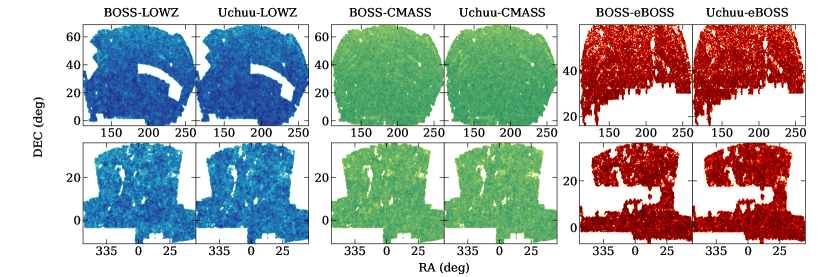
Figure 1: Sky area covered by the LOWZ, CMASS, and eBOSS data catalogues, and by the Uchuu-LOWZ, -CMASS, and -eBOSS lightcones. The upper and lower rows correspond to the northern and southern hemispheres, respectively. Colours indicate the angular number density normalized by the densest pixel. Darker colours indicate regions of higher density.

2 Galaxy data

We make use of various publicly available observational datasets, including the BOSS-LOWZ, BOSS-CMASS and eBOSS-LRG samples, encompassing both the Northern (N) and Southern (S) hemispheres. Furthermore, we analyse the combined BOSS-LOWZCMASS samples for both hemispheres. For convenience, we will subsequently refer to these datasets as LOWZ, CMASS, COMB, and eBOSS. Below, we describe in detail each of these samples. A summary of their global properties is given in Table 1.

Name	$z$-range	$N_{\mathrm{eff}}$	$A_{\mathrm{eff}}$	$N_{\mathrm{eff}}/A_{\mathrm{eff}}$	$V_{\mathrm{eff}}$
LOWZ-N	0.2$-$0.4	196186	5790	33.9	0.3633
LOWZ-S	0.2$-$0.4	91103	2491	36.6	0.1621
CMASS-N	0.43$-$0.7	605884	6821	88.8	1.2777
CMASS-S	0.43$-$0.7	225469	2525	89.3	0.4745
COMB-N	0.2$-$0.75	807900	5790	139.5	1.7208
COMB-S	0.2$-$0.75	352584	2491	141.5	0.7468
eBOSS-N	0.6$-$1.0	114004	2476	46.0	0.2584
eBOSS-S	0.6$-$1.0	71677	1627	44.1	0.1602

Table 1: Properties of the BOSS and eBOSS samples studied in this work. The first and second columns provide the sample name and the corresponding redshift range. The remaining columns give for each sample the (weighted) number of galaxies, the effective area (in $\,\mathrm{deg}^{2}$), the galaxy density in units of $\mathrm{deg}^{-2}$, and the effective volume (in $h^{-3}\mathrm{Gpc}^{3}$).

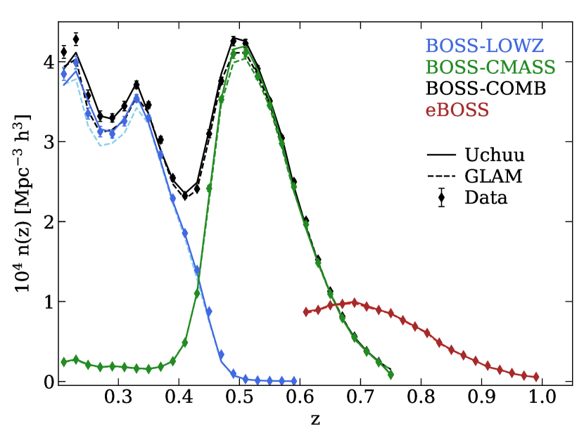
Figure 2: The comoving galaxy number density in the three samples studied: LOWZ in blue, CMASS in green, and eBOSS in red. The observational estimates are depicted using diamonds along with error bars. The mean $n(z)$ from both the Uchuu and GLAM-Uchuu lightcones are represented with solid and dashed lines, respectively (following the smoothing method described in the text). The error bars are obtained from the standard deviation of our set of 630 GLAM-Uchuu lightcones for each of the samples. Additionally, for illustrative purposes, the $n(z)$ of the BOSS-COMB sample is represented by a solid black line.

2.1 BOSS samples

We use the final data release of SDSS-III BOSS LRG (DR12; Alam et al., 2017), which contains the redshifts of 1 million LRG galaxies. This dataset covers an area of approximately $10,000$ deg², divided into two distinct subsets: LOWZ, designed for targeting LRGs up to $z\sim 0.4$, and CMASS, designed to target massive galaxies within the redshift range of $0.4<z<0.7$. Additionally, to maximize the effective volume covered by BOSS galaxies, a separate sample is constructed by combining the LOWZ and CMASS samples, denoted as the COMB sample. The spatial distribution and number density of these samples are shown in Figs. 1 and 2. The BOSS large-scale structure (LSS) catalogues are publicly available. For a more comprehensive understanding of the LOWZ and CMASS target selection criteria, and the creation of the COMB sample, we refer to Reid et al. (2015).

In these catalogues, as defined in Alam et al. (2017), a total weight is assigned to each galaxy $i$:

$$w_{\textrm{tot},i}=w_{\textrm{systot},i}(w_{\textrm{cp},i}+w_{\textrm{noz},i}-1),$$ (1)

where $w_{\textrm{systot}}$ is the total angular systematic weight, $w_{\textrm{cp}}$ is the fibre collision correction weight, and $w_{\textrm{noz}}$ is the redshift failure weight. This total galaxy weight must be used to obtain an unbiased estimation of the galaxy density field.

The geometry of the sky area covered by each LRG sample is precisely outlined using mangle format masks1. Regarding the BOSS-COMB sample, the mask is constructed to include every sector (each area covered by a unique set of plates) contained within the CMASS mask into the LOWZ counterpart. Furthermore, information regarding the BOSS fibre completeness is recorded within the mangle mask files. The completeness of every observed sector (indexed by $j$) is then defined as follows:

$$C_{\textrm{BOSS},j}=\frac{N_{\textrm{obs},j}+N_{\textrm{cp},j}}{N_{\textrm{star},j}+N_{\textrm{gal},j}+N_{\textrm{fail},j}+N_{\textrm{cp},j}+N_{\textrm{missed},j}},$$ (2)

where:

$N_{\textrm{gal},j}$ is the number of galaxies with redshifts from good BOSS spectra.

$N_{\textrm{star},j}$ is the number of spectroscopically confirmed stars.

$N_{\textrm{fail},j}$ is the number of objects with BOSS spectra for which stellar classification or redshift determination failed.

$N_{\textrm{obs},j}$ is defined as $N_{\textrm{obs},j}=N_{\textrm{gal},j}+N_{\textrm{star},j}+N_{\textrm{fail},j}$.

$N_{\textrm{cp},j}$ is the number of objects with no spectra, in a fibre collision group with at least one object of the same target class.

$N_{\textrm{missed},j}$ is the number of objects with no spectra, which, if in a fibre collision group, then there must be no other objects from the same target class.

On the edges of the survey there are regions of high incompleteness. To avoid these sectors, where a substantial fraction of redshifts is absent, sectors with $C_{\textrm{BOSS},j}<0.7$ are excluded and are not considered within the scope of this work.

The LSS catalogues for LOWZ and CMASS do not include galaxy stellar masses. We obtain this information from the lightcones presented in Rodríguez-Torres et al. (2016) and Kitaura et al. (2016). The observed LRG stellar mass functions (SMFs) are shown in the left and center panels of Fig. 3 for LOWZ and CMASS, respectively.

2.2 eBOSS LRG sample

We use the final data release of SDSS-IV eBOSS LRG (DR16; Prakash et al., 2016), which contains $\sim 200,000$ LRG over $4,000$ deg². This sample spans a higher redshift range than the CMASS sample, covering $0.6<z<1$ (Ross et al., 2020). The spatial distribution and number density of this eBOSS sample can be seen in Figs. 1 and 2. The final LSS catalogues for eBOSS are publicly available.

In these catalogues, the total weight for every galaxy, $i$, as described in Ross et al. (2020) is:

$$w_{\textrm{tot},i}=w_{\textrm{systot},i}~{}w_{\textrm{cp},i}~{}w_{\textrm{noz},i}.$$ (3)

where $w_{\textrm{systot},i}$, $w_{\textrm{cp},i}$, and $w_{\textrm{noz},i}$ are the same weights as described for BOSS.

The geometry of the sky area covered by the eBOSS sample is detailed within a mangle format mask2. The completeness for each sector is determined using the same methodology as employed for the BOSS samples. Following the observational systematics processing described in Ross et al. (2020), we apply a spectroscopic completeness threshold of $C_{\textrm{eBOSS},j}<0.5$ to exclude sectors with low completeness.

The SMF of the eBOSS galaxies is shown in the right panel of Fig. 3. Stellar masses are obtained from the data outputs provided by Comparat et al. (2017) through the use of the FIREFLY code applied to the DR16 eBOSS spectra. To avoid any overlap with the BOSS-CMASS LRGs, eBOSS adopted a specific magnitude cut of $i\geq 19.9$. This limit results in the most massive LRGs being excluded from the eBOSS sample. For details regarding the LRG selection, refer to Prakash et al. (2016).

3 Cosmological simulations

Simulation	$L_{\mathrm{box}}$	$N_{\mathrm{part}}$	$m_{\mathrm{part}}$	$h$	$\Omega_{\mathrm{m_{0}}}$	$\Omega_{\mathrm{\Lambda_{0}}}$	$\Omega_{\mathrm{b_{0}}}$	$\sigma_{8}$	$N_{\mathrm{g}}$	$\epsilon$	$z_{\mathrm{init}}$	$N_{\mathrm{s}}$	$N_{\mathrm{r}}$
Uchuu	2 000	$12~{}800^{3}$	$3.27\times 10^{8}$	0.677	0.309	0.691	0.0486	0.816	468 384	0.00427	127	5 570	1
GLAM-Uchuu	1 000	$2~{}000^{3}$	$1.06\times 10^{10}$	0.677	0.309	0.691	0.0486	0.816	5 800	0.172	104	136	630
GLAM-PMILL	1 000	$2~{}000^{3}$	$1.06\times 10^{10}$	0.678	0.307	0.693	0.0481	0.828	4 000	0.250	104	136	100
GLAM-PMILLnoBAO	1 000	$2~{}000^{3}$	$1.06\times 10^{10}$	0.674	0.307	0.693	0.0487	0.828	4 000	0.250	104	136	100
GLAM-Abacus	1 000	$2~{}000^{3}$	$1.09\times 10^{10}$	0.674	0.315	0.685	0.0493	0.812	7 500	0.133	104	136	100

Table 2: Numerical and cosmological parameters of the Uchuu and GLAM-Uchuu simulations used in this work. The columns give from left to right: the simulation name, size of the simulated box $L_{\mathrm{box}}$ in $\,h^{-1}\mathrm{Mpc}$, the number of particles $N_{\mathrm{part}}$, the mass the simulation particle $m_{\mathrm{part}}$ in $\,h^{-1}\mathrm{M_{\odot}}$ units, the cosmological parameters adopted in the simulation ($h$, $\Omega_{\mathrm{m_{0}}}$, $\Omega_{\mathrm{\Lambda_{0}}}$, $\Omega_{\mathrm{b_{0}}}$, $\sigma_{8}$), the mesh size $N_{\mathrm{g}}$, the gravitational softening length $\epsilon$ in $\,h^{-1}\mathrm{Mpc}$ units, the redshift of the initial linear power spectrum $z_{\mathrm{init}}$, the number of time-steps $N_{\mathrm{s}}$, and number of realizations $N_{\mathrm{r}}$.

Using the Uchuu and GLAM simulations listed in Table 2, we generate galaxy lightcones as well as lightcones for covariance errors for each of the analysed samples: LOWZ, CMASS, COMB and eBOSS. The goal of these lightcones is to faithfully reproduce the clustering statistics observed in the survey data.

Simulation	Sample	$N_{\mathrm{light}}$	$z$-range	$N_{\mathrm{eff}}$	$A_{\mathrm{eff}}$	$N_{\mathrm{eff}}/A_{\mathrm{eff}}$	$V_{\mathrm{eff}}$
Uchuu	LOWZ-N	2	0.2$-$0.4	193973	5751	33.7	0.36
	LOWZ-S	2	0.2$-$0.4	89944	2470	36.4	0.16
	CMASS-N	2	0.43$-$0.7	602206	6798	88.8	1.27
	CMASS-S	2	0.43$-$0.7	221921	2482	89.3	0.47
	COMB-N	2	0.2$-$0.75	806468	5751	140.2	1.71
	COMB-S	2	0.2$-$0.75	351348	2470	142.3	0.74
	eBOSS-N	2	0.6$-$1.0	113400	2462	46.1	0.26
	eBOSS-S	2	0.6$-$1.0	71424	1621	44.1	0.16
GLAM-Uchuu	LOWZ-N	630	0.2$-$0.4	188160	5751	32.7	0.36
	LOWZ-S	630	0.2$-$0.4	86194	2470	34.9	0.16
	CMASS-N	630	0.43$-$0.7	593339	6798	87.3	1.26
	CMASS-S	630	0.43$-$0.7	217727	6798	87.7	0.46
	COMB-N	630	0.2$-$0.75	787474	5751	136.9	1.69
	COMB-S	630	0.2$-$0.75	341650	2470	138.3	0.73
	eBOSS-N	630	0.6$-$1.0	112259	2462	45.6	0.25
	eBOSS-S	630	0.6$-$1.0	70510	1621	43.5	0.17

Table 3: Properties of the Uchuu and GLAM-Uchuu lightcones generated for each observational sample. The first column indicates the simulation used. The second and third columns provide the name and number of lightcones ($N_{\mathrm{light}}$) defining each sample dataset. The fourth column gives the redshift range considered for clustering studies. Subsequent columns provide the (weighted) mean number of galaxies, the mean effective area (in $\,\mathrm{deg}^{2}$), the mean density of galaxies per unit area (in $\mathrm{deg}^{-2}$), and the mean effective volume (in $h^{-3}\mathrm{Gpc}^{3}$).

3.1 The Uchuu Simulation

The Uchuu simulation is the largest run within the Uchuu suite (Ishiyama et al., 2021), tracing the evolution of $12,800^{3}$ dark matter particles, each with a mass of $3.27\text{\times}{10}^{8}\text{\,}{\mathrm{\mathit{h}}}^{-1}\text{\,}\mathrm{\mathrm{M}_{\odot}}$, within a periodic box of $2.0\text{\,}{\mathrm{\mathit{h}}}^{-1}\text{\,}\mathrm{Gpc}$. The adopted cosmological parameters adopted are $\Omega_{\mathrm{m_{0}}}=0.309$, $\Omega_{\mathrm{b_{0}}}=0.0486$, $\Omega_{\mathrm{\Lambda_{0}}}=0.691$, $h=0.677$, $n_{\mathrm{s}}=0.9667$, and $\sigma_{8}=0.816$, representing the best fitting CDM parameters corresponding to the Planck 2015 cosmology (Planck Collaboration et al., 2016). Employing the TreePM code GreeM (Ishiyama et al., 2009, 2012) with a gravitational softening length of $4.27\text{\,}{\mathrm{\mathit{h}}}^{-1}\text{\,}\mathrm{kpc}$, Uchuu tracks the gravitational evolution of particles from redshift $z=127$ to $z=0$. A total of 50 particle snapshots were stored within the redshift interval $z=0$ to $z=14$. The identification of bound structures was performed using the Rockstar phase-space halo/subhalo finder (Behroozi et al., 2013a); subhalos in Uchuu are $90\%$ complete down to $V_{\mathrm{peak}}\gtrsim$70\text{\,}\mathrm{km}\text{\,}{\mathrm{s}}^{-1}$$, while distinct halos are $90\%$ complete down to $V_{\mathrm{peak}}\gtrsim$50\text{\,}\mathrm{km}\text{\,}{\mathrm{s}}^{-1}$$. Merger trees were then constructed using the Consistent Trees code (Behroozi et al., 2013b). The properties of the Uchuu simulation are summarized in Table 2.

The high resolution of the Uchuu simulation makes it optimal for generating simulated galaxy lightcones. Uchuu is able to resolve dark matter halos and subhalos down to small masses, a key requirement for employing the SHAM. This capability results in high completeness, in terms of the fraction of galaxies resolved, particularly at lower redshift. Furthermore, the large volume of Uchuu allows us to study large-scale clustering features, such as the BAO.

3.2 The GLAM simulations

The GLAM simulations (Klypin & Prada, 2018) are $N$-body cosmological simulations that follow the evolution of $2000^{3}$ dark matter particles, each having a particle mass of $1.06\text{\times}{10}^{10}\text{\,}{\mathrm{\mathit{h}}}^{-1}\text{\,}\mathrm{\mathrm{M}_{\odot}}$. All GLAM boxes are $1.0\text{\,}{\mathrm{\mathit{h}}}^{-1}\text{\,}\mathrm{Gpc}$ comoving periodic boxes, with $N_{\rm s}=136$ time-steps and a mesh of $N_{\rm g}=5,800$ cells per side, resulting in a spatial resolution of $0.172\,h^{-1}\mathrm{Mpc}$. The initial conditions are generated using the Zeldovich approximation starting at $z_{\mathrm{ini}}=104$. Due to the lower resolution of these simulations compared to Uchuu, the GLAM simulations are only capable of correctly resolve distinct halos (not subhalos) with virial masses greater than $10^{12}\,h^{-1}\mathrm{M_{\odot}}$ (Hernández-Aguayo et al., 2021).

The GLAM simulations have been run assuming different cosmologies. The numerical and cosmological parameters adopted in these simulations are listed in Table 2 and summarized below:

• GLAM-Uchuu: Adopts the same Planck cosmology (PL15) and linear power spectrum as the Uchuu simulation.

• GLAM-PMILL and -PMILLnoBAO: Adopt the cosmological parameters assumed in the Planck Millennium simulation (PMILL; Baugh et al., 2019), which uses the best-fitting CDM parameters from the first Planck 2013 data release (PL13; Planck Collaboration et al., 2014). In PMILLnoBAO, an initial power spectrum corresponding to a matter distribution without baryonic acoustic oscillations is used, resulting in the absence of the BAO feature in these realisations.

• GLAM-Abacus: Adopts the abacus$\_$cosm000 cosmology from the AbacusSummit $N$-body simulation suite (Maksimova et al., 2021), which includes the effect of massive neutrinos.

4 Constructing the Uchuu-LRG lightcones

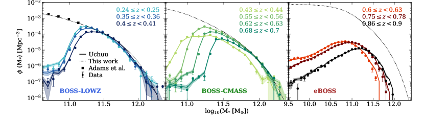
Figure 3: The observed LRG SMF (points) in the LOWZ (left panel), CMASS (middle panel), and eBOSS (right panel) samples. The mean SMF of the Uchuu-LRG lightcones are shown using solid lines. We show the SMF for several redshift bins within the relevant redshift ranges for each sample, using a colour scheme indicated in each plot. The dotted curves show the complete SMFs adopted for the implementation of the SHAM method (see Table 4), while the square points denote the PRIMUS data taken from Moustakas et al. (2013) (see Section 4.1). Data error bars represent the standard deviation, 1-$\sigma$, of our set of GLAM-Uchuu LRG lightcones, while the shaded area for Uchuu represents the error on the mean, $\sigma/\sqrt{2}$.

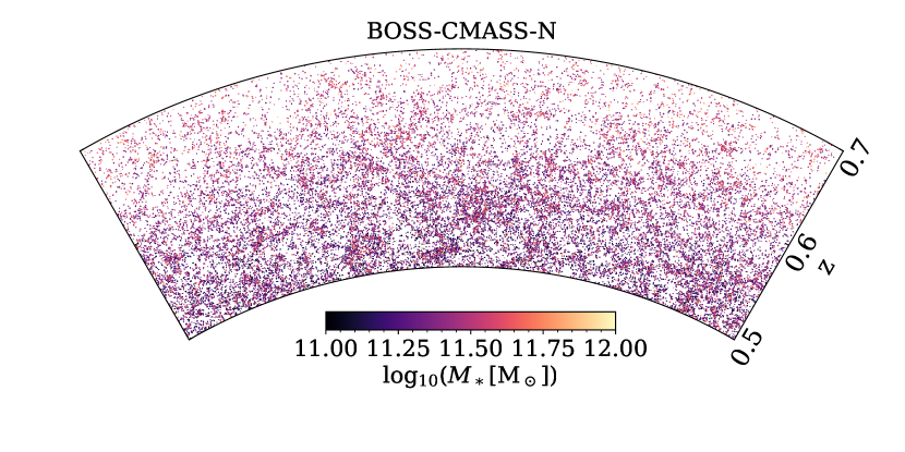
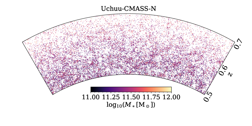
Figure 4: Slices through the CMASS-N sample (left), and the Uchuu-CMASS-N lightcone (right), with galaxies colour-coded according their stellar mass as indicated in the legend. The displayed galaxies fall within the range of $10<\mathrm{dec}<30~{}\deg$, and $150<\mathrm{RA}<210~{}\deg$.

We will now outline the procedure employed to create LRG lightcones from the Uchuu simulation. This includes details about the SHAM method, modelling of the LRG stellar mass incompleteness, handling angular masks, and addressing fibre collisions. For each of the analyzed samples, we generate two independent lightcones by duplicating the survey footprint across the sky, resulting in a total of 16 lightcones. The properties of the Uchuu lightcones are shown in Table 3.

To capture the redshift evolution of the galaxy clustering, we use a series of Uchuu snapshots. For each sample, the redshifts of the boxes used are:

LOWZ:   $z=0.19,0.25,0.30,0.36,0.43$

CMASS: $z=0.43,0.49,0.56,0.63,0.7$

eBOSS:   $z=0.63,0.7,0.78,0.86$

Fig. 4 shows a comparison between a slice of the CMASS-N galaxy distribution in the observations (left panel) and the corresponding Uchuu-LRG lightcone (right panel). Individual galaxies are colour-coded based on their stellar mass, highlighting the consistency between our simulated lightcones and the observed data. The decrease in galaxy density with increasing redshift matches the observed redshift distribution $n(z)$ in this particular sample (see Fig. 2).

4.1 Stellar mass assignment

We adopt the SHAM method to populate galaxies within the dark matter halos and subhalos in each Uchuu simulation box. This technique assumes a monotonic relation between the stellar mass of galaxies and a specific property of the associated halo, which is a proxy of its mass, thereby assigning more massive galaxies to more massive (sub)halos (Guo et al., 2016). In the standard SHAM approach, there is no distinction between halos and subhalos, since the assignment is only based on a subhalo property and not the environment of the subhalo (although the method has been extended to include such information, see Contreras et al. 2021).

For the SHAM technique, we use the peak value of the maximum circular velocity over the history of the (sub)halo, $V_{\mathrm{peak}}$, as a proxy for the mass. This choice of property has been shown to yield galaxy catalogues that exhibit better agreement with observational data (as discussed in Trujillo-Gomez et al., 2011; Reddick et al., 2013; Guo et al., 2016). Several reasons underpin this improvement: i) circular velocity parameters are typically reached at one-tenth of the (sub)halo’s radius, which provides a more accurate characterization of the scales directly influencing galaxies (Chaves-Montero et al., 2016); ii) $V_{\mathrm{peak}}$ is better defined for both halos and subhalos when compared to halo mass, as the latter becomes ambiguous for subhalos. Furthermore, subhalo mass is also influenced by the choice of halo finder, as it depends on a code-defined truncation radius at which the particles are defined as unbound and are removed (Trujillo-Gomez et al., 2011). iii) the circular velocity is less affected than a mass measurement by the mass loss experienced by a halo or subhalo after it becomes part of a large structure (Kravtsov et al., 2004; Hayashi et al., 2003).

It is important to note that while the original SHAM approach assumes a monotonic relation between the galaxy stellar mass and $V_{\mathrm{peak}}$, observations suggest that this assignment cannot be strictly one-to-one. To achieve more realistic results, it becomes necessary to introduce scatter into the abundance matching process (e.g. Skibba et al., 2011; Trujillo-Gomez et al., 2011). We adopt the scatter scheme proposed in Rodríguez-Torres et al. (2016), which defines the scattered $V_{\mathrm{peak}}$ as the abundance matching parameter:

$$V_{\mathrm{peak}}^{\mathrm{scat}}=(1+\mathcal{N}(0,\sigma_{\mathrm{SHAM}}))V_{\mathrm{peak}},$$ (4)

where $\mathcal{N}$ represents a Gaussian-distributed random number with a mean of zero and standard deviation $\sigma_{\mathrm{SHAM}}$ (the SHAM scatter parameter). The optimal values for the scatter parameters are determined by optimizing the goodness-of-fit between the two-point correlation functions measured from the observational samples and those obtained from the Uchuu lightcones. Note that the footprint and number density of these lightcones are set beforehand to match the data, as described in Section 4.3. The mean SHAM scatter parameters over the boxes of each sample are as follows: $\overline{\sigma}_{\mathrm{LOWZ}}=0.26$, $\overline{\sigma}_{\mathrm{CMASS}}=0.30$, $\overline{\sigma}_{\mathrm{eBOSS}}=0.65$, all in agreement with previous work (see Rodríguez-Torres et al., 2016; Nuza et al., 2013; Yu et al., 2022). We note that these values increase with redshift. The scatter is not necessarily directly linked to redshift. However, redshift could influence the halo-galaxy connection due to the dynamic processes of galaxy formation and evolution. In addition, as redshift values increase, observations might encounter higher levels of noise and limitations from instruments. The inferred value for the eBOSS scatter parameter seems substantially higher than the values recovered for the other samples which may indicate that it is influenced by the high incompleteness in the SMF for this sample.

In order to implement the SHAM technique in the Uchuu boxes, we require a complete SMF, which accurately represents a complete population of galaxies prior to applying any of the magnitude and colour selections specific to the LRG samples considered here. Due to the selection function in the BOSS and eBOSS surveys, the SMF becomes incomplete in these samples at low masses (see Fig. 3). For CMASS and eBOSS we adopt the Schechter function taken from Rodríguez-Torres et al. (2016) as the complete SMF, which is shown by the dashed line in Fig. 3. These authors combine the CMASS SMF, which is complete at higher stellar masses, with the SMF from the PRIMUS survey at lower masses (Moustakas et al., 2013). In the case of LOWZ, we also incorporate the averaged SMF measurements from PRIMUS for the redshift ranges $0.2<z<0.3$ and $0.3<z<0.5$ (square symbols). Subsequently, we perform a fit to both data sets using a Schechter function. All the fits are shown as dotted lines in Fig. 3. The fitted parameters are given in Table 4.

Sample	Mass range	$10^{3}~{}\phi_{\ast}$	$\alpha$	log10 $M_{\ast}$
LOWZ	$M_{\ast}\leq~{}10^{11.3}$	$2.894$	$-0.996$	$10.82$
	$M_{\ast}>~{}10^{11.3}$	$0.476$	$-1.557$	$11.23$
CMASS $\&$ eBOSS	$M_{\ast}\leq~{}10^{11.0}$	$4.002$	$-0.938$	$10.76$
	$M_{\ast}>~{}10^{11.0}$	$0.266$	$-2.447$	$11.42$

Table 4: Fitted parameters of the Schechter functions adopted in this work as complete SMFs for the LOWZ, CMASS, and eBOSS samples. The characteristic stellar mass, $M_{\ast}$, is given in units of $M_{\odot}$, and $\phi_{\ast}$ is given in units of Mpc${}^{-3}~{}(\log_{10}M_{\ast})^{-1}$

.

Once we have the complete SMF fits and the values of $V_{\mathrm{peak}}^{\mathrm{scat}}$ for each halo and subhalo in Uchuu (i.e. after including the scatter), we are able to apply the SHAM technique. The procedure is as follows:

1. Compute the cumulative number density of (sub)halos as a function of decreasing $V_{\mathrm{peak}}^{\mathrm{scat}}$, i.e. the scattered value of the circular velocity.

2. Compute the cumulative number density of galaxies as a function of decreasing stellar mass, $M_{\ast}$, using the adopted complete SMF.

3. Construct a monotonic relation between the cumulative number density functions from steps (i) and (ii):

   $$n_{\mathrm{gal}}(>M_{\ast})=n_{\mathrm{halo}}(>V^{\mathrm{scat}}_{\mathrm{peak}}),$$ (5)

   which implies that a (sub)halo with $V^{\mathrm{scat}}_{\mathrm{peak},i}$ will contain a galaxy with stellar mass $M_{\ast,i}$, assigning the most massive galaxy to the (sub)halo with the highest $V^{\rm scat}_{\rm peak}$. We note that this assignment is monotonic between $V^{\mathrm{scat}}_{\mathrm{peak}}$ and $M_{\ast}$, but not between $V_{\mathrm{peak}}$ and $M_{\ast}$.

4. Repeat this sequence for every Uchuu box.

The next step is to model the incomplete stellar mass distribution observed in all samples. For Uchuu-LOWZ and -CMASS galaxy boxes, we do this by randomly down-sampling galaxies from the complete SMFs. The approach is different for the case of eBOSS, as the SMF is highly incomplete in this instance for the whole stellar mass range (see the right panel of Fig. 3). To account for this effect, we rely on the results presented in Alam et al. (2020), where they report that the probability of a distinct halo containing a central LRG is at most 30$\%$. Therefore, after applying the SHAM on the Uchuu-eBOSS boxes, we randomly select 30$\%$ of the galaxies. The remainder of the observed incompleteness, primarily located at the lower end of stellar masses, is acquired through the same methodology as applied in the LOWZ and CMASS samples. The final SMFs of our Uchuu-LRG lightcones are shown by the solid curves in Fig. 3. We validate our scheme for assigning stellar masses to galaxies by measuring the galaxy clustering in the lightcones as a function of stellar mass, as described below.

4.2 Creating the lightcones by joining the cubic boxes

The next step in the production of the Uchuu lightcones involves joining the cubic boxes, that have been populated with galaxies, into spherical shells (see Smith et al., 2022, for a detailed description of this method).

First, we position the observer at $(0,0,0)\,h^{-1}\mathrm{Gpc}$ in comoving coordinates and transform the Cartesian coordinates (x,y,z) of each galaxy within the cubic box to redshift-space coordinates (RA,dec,z), considering the effect of galaxy peculiar velocities. Each box is then divided into spherical shells, where the comoving distance between the observer and the inner/outer edges of the shell corresponds to the redshift that lies midway between this snapshot and the next/previous snapshot. These spherical shells are then joined together to build three full-sky lightcones: Uchuu-LOWZ, -CMASS and -eBOSS. To cover their sky areas, it becomes necessary to periodically replicate the corresponding galaxy cubic boxes at specific redshift ranges. If the centre of a halo lies within a given spherical shell, the entire halo is included in the lightcone. However, if a halo partially extends into a shell but its center fall outside the shell, it is excluded from the lightcone.

4.3 Radial selection function and angular mask

We randomly downsample the galaxy population in the redshift ranges where the lightcone’s $n(z)$ surpasses the observed one. By doing this, we also implement a smooth transition between the spherical shells, avoiding a sudden step-like behaviour. The redshift distribution of galaxies in the Uchuu lightcones resulting from this process are shown by the solid lines in Fig. 2.

We proceed to match the sky area of the full-sky Uchuu lightcones with that of the observed samples, using the available survey masks (see Sections 2.1 and 2.2). Additionally, we apply various veto masks. These include masks for bright stars, bright objects, and non-photometric conditions (in the real data). Moreover, we incorporate veto masks based on the seeing during the imaging data acquisition and Galactic extinction (avoiding high-extinction areas), see Ross et al., 2017 and Ross et al., 2020 for details. The result of applying these masks and the comparison with observed data is shown in Fig. 1. To improve our statistics and benefiting from our lightcones (without masks) covering the whole sky area, we repeat this procedure once more time by shifting the sky position of the masks by $180$ deg. By doing this, we are able to obtain two independent Uchuu lightcones for each sample.

As shown in Table 3, the effective area of the Uchuu lightcones is slightly smaller than that of the actual data ($\sim 1\%$ lower). The angular geometry of the samples is represented by mangle polygons, which lack the finest angular footprint details, contributing to this minor variation in the effective area.

4.4 Completeness and fibre collisions

A final step is required to fully replicate the observed samples, which involves the incorporation of survey systematics. This includes the angular completeness of the masks, $C$, defined in Equation 2. To account for this property, we downsample the regions where the completeness falls below one, retaining only those regions where $C\geq~{}0.7$ for Uchuu-LOWZ and -CMASS, and $C\geq~{}0.5$ for Uchuu-eBOSS.

Another observational artefact is the so-called fibre collisions. This is due to the finite size of the fibre-head on the plate. If two galaxies are separated by less than 62 arcsec apart (which represents the fibre collision radius), it is possible that only one of these galaxies will be assigned a spectroscopic fibre, resulting in the inability to determine the redshift of the other galaxy (Reid et al., 2015). The distribution of such closely spaced galaxy pairs is expected to be correlated with galaxy density. To model this effect, we adopt the method described in Guo et al. (2012), where the main goal is to divide the complete galaxy sample into two distinct populations:

Population 1 (P1): A subsample where no galaxy is within the fibre collision radius of any other galaxy within this same subsample.

Population 2 (P2): A subsample including all galaxies that are not of P1. Every galaxy in this population lies within the fibre collision radius of a galaxy in P1. All the galaxies affected by fibre collisions belong to this subsample.

The procedure for creating these two populations is as follows:

1. Initially, all galaxies in the lightcone are designated as members of P1.

2. For each pair of collided galaxies in P1, we randomly select one galaxy to be reassigned to P2.

3. For each group of three or more collided galaxies in P1, we chose the galaxy that collides with the most P1 galaxies and assign it to P2.

4. We repeat steps (ii) and (iii) until no galaxies in P1 collides with each other.

Once the two populations have been created, we proceed to randomly select from P2 the galaxies that will not be observed. We do this for all the Uchuu lightcones, resulting in the final percentages of fibre-collided galaxies as follows: $1.3\%$ ($2.9\%$) for LOWZ-N (S) lightcones, $5.0\%$ ($4.3\%$) for CMASS, and $3.4\%$ ($3.5\%$) for eBOSS, which match the values in the observed samples (Reid et al., 2015). Once the unobserved galaxies are determined, we simply assign higher weights to the nearest galaxies that were assigned fibres, accounting for collided galaxies that were not assigned fibres (Nearest Neighbour Weights, NNW).

The NNW method, however, has a drawback: it ignores the correlation between observed and unobserved targets. To address this correlation properly, an approach known as the ‘pairwise inverse probability’ (PIP) weighting scheme was proposed by Bianchi & Percival (2017). This method has been applied to the eBOSS data as demonstrated in Mohammad et al. (2020). While the authors acknowledged the challenges involved in the PIP process, they also noted that approximate methods like NNW yield sufficiently accurate results considering the statistical uncertainties present in the data. Moreover, applying PIP weights for the BOSS samples would require further information that is not publicly available. Given these considerations, we have decided not to apply PIP weights to our lightcones. It is on scales smaller than $1\,h^{-1}\mathrm{Mpc}$ where these weights could have the most significant impact. Consequently, we may expect discrepancies in the clustering of galaxies at these pair separations between the results from observations and simulations.

4.5 The Uchuu-COMB lightcone

We now describe the process of generating the Uchuu-COMB lightcones. To achieve this, we combine our Uchuu-LOWZ and -CMASS lightcones and apply the corresponding COMB mangle mask. When combining galaxy populations with different clustering amplitudes, it is optimal to assign weights to each sample to account for these differences (Percival et al., 2004). In this work, we count the number of galaxy pairs for various redshift bins within each sample. We then normalize these values, and adopt them as the weight for galaxies within that redshift range and sample.

5 Constructing the GLAM-Uchuu covariance lightcones

To estimate covariance errors, we need to significantly increase the number of simulated lightcones. In this section, we detail the construction of the GLAM-Uchuu covariance lightcones: a set of $630\times 8$ lightcones derived from the GLAM-Uchuu $N$-body simulations for each of the LRG samples. The methodology employed for generating these lightcones is described below, while the properties of the produced covariance lightcones are presented in Table 3.

Similarly to the Uchuu lightcones, we use several snapshots from the GLAM simulations to reproduce the redshift-dependent evolution of galaxy clustering. We select the GLAM boxes that closely match redshifts of the corresponding Uchuu snapshots:

LOWZ:   $z=0.20,0.27,0.31,0.37,0.46$

CMASS: $z=0.46,0.49,0.564,0.62,0.72$

eBOSS:   $z=0.62,0.72,0.79,0.86$

5.1 Halo occupation distribution

As described in Section 3.2, the GLAM simulations do not resolve substructure inside distinct halos. Therefore, the SHAM method discussed in Section 4.1 cannot be directly applied to populate galaxies within halos in the GLAM simulations. Instead, a statistical method using the halo occupancy of galaxies from the Uchuu LRG catalogues must be employed. The HOD describes the mean number of galaxies within a distinct halo of virial mass $M_{\mathrm{halo}}$, which can be written as the sum of the mean number of central and satellite galaxies:

$$\langle N_{\mathrm{gal}}(M_{\mathrm{halo}})\rangle=\langle N_{\mathrm{cen}}(M_{\mathrm{halo}})\rangle+\langle N_{\mathrm{sat}}(M_{\mathrm{halo}})\rangle.$$ (6)

In this context, we obtain the HOD from the Uchuu galaxy cubic boxes we construct in Section 4.1. This is possible because each galaxy provides information whether it is a central or satellite, as well as the mass of the distinct halo it inhabits. We then use the set of 630 GLAM-Uchuu halo cubic boxes available at each redshift to generate galaxy catalogues. In this process, we randomly select galaxies for each distinct halo, following the corresponding HOD as determined from the Uchuu-LRG samples. The Uchuu-LRG HODs for LOWZ, CMASS and eBOSS are shown in Section 6.2. GLAM-Uchuu simulations resolve halos with masses within $10^{12}$ and $10^{15}$. While the HODs obtained from the Uchuu-LRG samples do not extend significantly outside this mass range, our GLAM-Uchuu boxes end up having a marginal deficit of galaxies compared to Uchuu due to their incompleteness (and not-well resolved halos) below $\sim 10^{12.5}$ and above $\sim 10^{14.5}$. This effect is visible in Table 3 (and Fig. 2), where the GLAM $N_{\mathrm{eff}}$ ($n(z)$) is slightly below that of the data and Uchuu.

5.2 Stellar mass assignment and generation of lightcones

The galaxies added into the GLAM-Uchuu boxes do not have assigned stellar masses. Unlike the SHAM approach, which inherently accounts for this property, we must incorporate stellar masses independently. To achieve this, we derive the probability distribution of central and satellite stellar masses from Uchuu galaxy boxes across various ranges of distinct halo masses. These distributions are then employed to determine the stellar masses of the GLAM galaxies. The resulting SMFs are, as designed, consistent with those of Uchuu.

The subsequent step in generating the GLAM-Uchuu LRG lightcones involves joining the galaxy boxes into spherical shells and smoothing their number density, $n(z)$. This procedure is explained in Sections 4.2 and 4.3. By applying the available survey and veto masks, we match the area of the lightcones to that of the observed samples (without shifting the sky position of the masks). As a last step, following the process described in Section 4.4, we account for survey systematics. The creation of the GLAM-Uchuu-COMB lightcones follows the steps described in Section 4.5.

6 Results

In this section, we present the results of the galaxy clustering analysis conducted both in configuration and Fourier space. These analyses require the application of appropriate weights to both the data and the simulated lightcones.

For the LOWZ, CMASS and COMB data, we apply the $w_{\textrm{tot},i}$ weights as outlined in Equation 1. The weights used for the eBOSS data are specified in Equation 3. Incorporating the fibre collision weights, described in Sections 4.4 & 5.2, is essential for the Uchuu and GLAM-Uchuu lightcones. To enhance the signal-to-noise ratio of the clustering measurements, galaxies from both the data and lightcones are additionally weighted based on the galaxy number density, $n(z)$, using the weights introduced by Feldman et al. (1994) (hereafter FKP weights):

$$w_{\textrm{FKP}}=\frac{1}{1+n(z)P_{\textrm{FKP}}}.$$ (7)

We set $P_{\textrm{FKP}}=10~{}000~{}h^{-3}\mathrm{Mpc}^{3}$, which is close to the value of the BOSS and eBOSS LRG power spectrum at $\mathrm{k}=0.1\,h^{-1}\mathrm{Mpc}$, the scale where we aim to minimize the variance (see Ross et al., 2017, 2020). The $n(z)$ is estimated for each case from either the data or the lightcones. The random catalogs required for these analyses are obtained from the SDSS-BOSS Science Archive Server and SDSS-eBOSS Science Archive Server. Randoms are weighted only by FKP weights.

The redshift ranges considered for each sample, as well as those shown in the following figures, are listed in Table 1: $0.2<z<0.4$ for LOWZ, $0.43<z<0.7$ for CMASS, and $0.6<1.0$ for eBOSS. In the case of COMB galaxies, we adopt the same analysis scheme as presented by Alam et al. (2017), and consider three redshift ranges: $0.2<z<0.5$, $0.4<z<0.6$ and $0.5<z<0.75$.

6.1 Testing the Planck cosmology against the data with Uchuu

In this section, we assess the performance of our theoretical predictions, derived from the Planck cosmology as determined from our Uchuu lightcones, to reproduce the observed data. We start by studying the LOWZ-, CMASS- and eBOSS-N samples, and conclude with an evaluation of the COMB-N$+$S sample.

6.1.1 Clustering in configuration and Fourier space

We first study the anisotropic two-point correlation function (2PCF) in redshift space, $\xi(s,\mu)$, which is computed using the Landy-Szalay estimator estimator Landy & Szalay (1993). We refer to the observed or simulated data galaxies as $D$ and the random galaxies as $R$:

$$\xi(s,\mu)=\frac{\mathrm{DD}(s,\mu)-2\mathrm{DR}(s,\mu)+\mathrm{RR}(s,\mu)}{\mathrm{RR}(s,\mu)},$$ (8)

where $s$ represents the redshift-space separation between a pair of objects in units of $\,h^{-1}\mathrm{Mpc}$, $\mu$ is the cosine of the angle between the pair separation vector and the line-of-sight, and $\mathrm{DD}$, $\mathrm{DR}$ and $\mathrm{RR}$ are the normalized pair counts of the galaxy-galaxy, galaxy-random and random-random catalogues, respectively. For a more exhaustive analysis, we decompose $\xi(\mathrm{s},\mu)$ into its Legendre multipoles:

$$\xi_{\ell}(\mathrm{s})=\frac{2\ell+1}{2}\int^{1}_{-1}\xi(\mathrm{s},\mu)P_{\ell}(\mu)\mathrm{d}\mu,$$ (9)

where $P_{\ell}(\mu)$ is the $\ell th$ Legendre Polynomial.

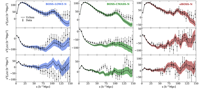
((a)) Large scale.

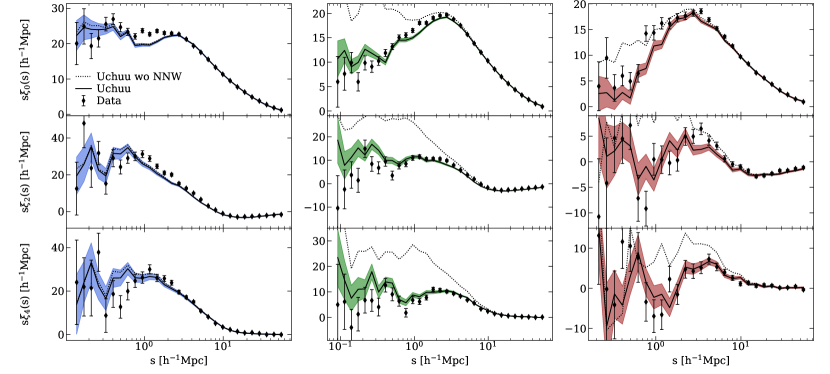
((b)) Small scale.

Figure 5: Measurements of the monopole, quadrupole and hexadecapole moments of the 2PCF are presented in the first, middle and bottom rows, respectively, for CMASS-N, LOWZ-N and eBOSS-N, arranged from left to right in the columns. Observational measurements are shown by data points, while the solid lines show the mean 2PCF derived from the Uchuu lightcones. Data error bars represent the standard deviation of our set of GLAM-Uchuu lightcones at the 1-$\sigma$ level, whereas the shaded area for Uchuu indicates the error on the mean $\sigma/\sqrt{2}$. Panel (a) shows the 2PCF measurements spanning from $0$ to $150\,h^{-1}\mathrm{Mpc}$ in bins of $5\,h^{-1}\mathrm{Mpc}$. Panel (b) presents the results up to $60\,h^{-1}\mathrm{Mpc}$ in bins equally spaced in the logarithm of pair separation. For reference, the mean Uchuu 2PCF without fibre collision correction (NNW) is depicted with dotted lines.

In Fig. 5, we present the monopole ($\ell=0$), quadrupole ($\ell=2$) and hexadecapole ($\ell=4$) moments of the 2PCF for the three samples: LOWZ, CMASS and eBOSS-N. The results include both observed data and theoretical predictions determined from the mean of the Uchuu lightcones. Overall, our Uchuu lightcones are able to reproduce the clustering measurements obtained from the observed data, showcasing remarkable accuracy in certain samples. Residuals from the 2PCF monopole, denoted as $r=\xi_{0}^{\mathrm{Uchuu}}/\xi_{0}^{\mathrm{data}}-1$, maintain values under $2.5\%$ across all samples ranging from the fibre collision scale up to $25\,h^{-1}\mathrm{Mpc}$. Within the range of $100\,h^{-1}\mathrm{Mpc}$, residuals remain below $10\%$ for LOWZ and CMASS, and under $15\%$ for eBOSS. We define the fibre collision scale as the $s$-value at which the ratio between the multipoles of Uchuu with and without NNW is greater than $2\%$: $2.3\,h^{-1}\mathrm{Mpc}$ in LOWZ, $4.2\,h^{-1}\mathrm{Mpc}$ in CMASS, and $6.5\,h^{-1}\mathrm{Mpc}$ in eBOSS. We set these scales as the minimum since below this value, the accuracy of our results decreases.

Beyond the BAO scale ($\mathrm{s}\geq 120\,h^{-1}\mathrm{Mpc}$), significant fluctuations become apparent due to cosmic variance. At the smallest scales, below $\sim 1\,h^{-1}\mathrm{Mpc}$, deviations between the measurements from the lightcones and the observed data can be attributed to the non-application of the PIP weights in the lightcones, as mentioned in Section 4.4. Notably, there are differences between the results by more than 1-$\sigma$ for some scales above $60\,h^{-1}\mathrm{Mpc}$. Moreover, while our Uchuu lightcones monopole cross zero after BAO peak, the observations do not. It is widely recognized that, at large scales, the measurements are significantly influenced by observational systematics. Huterer et al. (2013) conducted an exhaustive investigation into photometric calibration errors and their repercussions on clustering measurements, illustrating that calibration uncertainties consistently give rise to large-scale power variations. The significance and potential causes of the large-scale excess are studied also in Ross et al. (2017), where they demonstrate that it has no significant impact on BAO measurements. Their findings indicate that these measurements remain resilient, both in lightcones and the data, regardless of whether or not any weights are included. Reader may also discern some differences between the results for the multipole moments that cannot be accounted for by the aforementioned reasons, such as the CMASS quadrupole. Exploring variations of the only free parameter in the SHAM, $\sigma_{\mathrm{SHAM}}$, does not seem to meaningfully impact the shape multipoles, suggesting that the observed discrepancies are most likely a result of statistical fluctuation. This hypothesis is supported by the improved performance of our 630 GLAM-Uchuu lightcone sets (see Section 6.2). All the highlighted trends (including the CMASS quadrupole behavior) are in agreement with results presented in e.g. Rodríguez-Torres et al. (2016), Kitaura et al. (2016) or Ross et al. (2017).

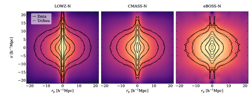
Figure 6: The mean 2PCF_2d from Uchuu-LOWZ-N (left column), -CMASS-N (middle column), and -eBOSS-N lightcones (right column) is plotted as a function of pair separation perpendicular ($r_{\mathrm{p}}$) and parallel ($\pi$) to the line-of-sight. To illustrate deviations from circular symmetry, the first quadrant is replicated with reflections in both axes. Contours of the 2PCF_2d estimated from the observations and from Uchuu are displayed as black solid and dashed curves, respectively. The contour levels shown are $[0.5,0.8,2,4,8,20]$.

Using the Landy-Szalay estimator, we now compute the two-dimensional (2d) 2PCF, $\xi(r_{\mathrm{p}},\pi)$, where $r_{\mathrm{p}}$ and $\pi$ represent the pair separations perpendicular and parallel to the line-of-sight, respectively. The results are presented in Fig. 6, where the mean 2PCF_2d derived from Uchuu-LOWZ, -CMASS, and -eBOSS-N lightcones is shown in the left, middle, and right columns, respectively. Solid curves represent the contours estimated from the observed data, while dashed curves depict the contours from Uchuu.

The 2PCF_2d is the simplest statistical measure of peculiar velocities the in cosmological structure. This function remains directionally independent in an isotropic universe. However, this property does not hold in redshift space, where only radial separations, $\pi$, are distorted by the peculiar velocities of the galaxies. This distortion is commonly referred to as redshift space distortions (RSD). The impact of RSD is particularly prominent on small scales, such as within galaxy groups and clusters, leading to the well-known “fingers-of-God” effect visible in cone plots showing galaxy positions (Peacock et al., 2001). The results shown in Fig. 6 clearly exhibit the presence of RSD, evident by the elongations along the $\pi$-axis at scales within $5\,h^{-1}\mathrm{Mpc}$. The remarkable agreement between our Uchuu lightcones and the BOSS/eBOSS data is noteworthy. Minor deviations on small scales, related to the non-use of PIP weights, are consistent with the previous results shown in Fig. 5.

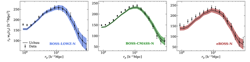
Figure 7: Measurements of the 2PCF for CMASS-N (left column), LOWZ-N (middle column) and eBOSS-N (right column). Measurements from observations are shown by data points, while the solid lines represent the mean 2PCF derived from the Uchuu lightcones. Data error bars represent the standard deviation of our set of GLAM-Uchuu lightcones, 1-$\sigma$, while the Uchuu shaded area is the error on the mean, calculated as $\sigma/\sqrt{2}$. The 2PCF is measured up to $100\,h^{-1}\mathrm{Mpc}$ in equally-spaced logarithmic bins.

As mentioned above, the impact of RSD only affects the pair separation along the line-of-sight ($\pi$). Therefore, these distortions can be removed by projecting $\xi(r_{\mathrm{p}},\pi)$ onto the $\pi$-axis (Davis & Peebles, 1983; Norberg, Baugh, Gaztañaga & Croton, 2009) as follows:

$$w_{\mathrm{p}}(r_{\mathrm{p}})=\int_{-\infty}^{+\infty}\xi(r_{\mathrm{p}},\pi)\mathrm{d}\pi.$$ (10)

In practice, this integral is truncated at a certain $\pi_{\mathrm{max}}$. In this work, we adopt $\pi_{\mathrm{max}}=80\,h^{-1}\mathrm{Mpc}$. The projected correlation functions (pCF) are shown in Fig. 7. The agreement between the theoretical predictions determined from the mean of the Uchuu lightcones and the observational estimates aligns with the expectations from Fig. 6.

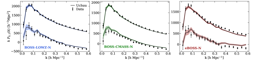
Figure 8: Measurements of the power spectrum monopole (upper curve) and quadrupole (lower curve, lighter shading) for CMASS-N (left column), LOWZ-N (middle column) and eBOSS-N (right column). Observed data measurements are represented by data points. The solid lines represent the mean power spectrum derived from the Uchuu lightcones. Data error bars represent the standard deviation of our set of GLAM-Uchuu lightcones, 1-$\sigma$, while the Uchuu shaded area indicates the error on the mean, $\sigma/\sqrt{2}$. The power spectra are measured from $\mathrm{k}=0.005$ to $0.6\,h\mathrm{Mpc}^{-1}$ in $0.03\,h\mathrm{Mpc}^{-1}$ bins.

In a final test, we measure the power spectrum monopole, $P_{0}(k)$ and quadrupole, $P_{2}(k)$, which can be calculated following Equations 2 to 7 from Feldman, Kaiser & Peacock (1994). These calculations have been carried out using the Python package pypower, which implements the Hand et al. (2017) estimator. This estimator takes coordinate-space positions at mesh nodes and directly computes the normalisation factor from the mesh. To mitigate the impact of aliasing, we employ a piecewise cubic spline (PCS) mesh assignment scheme with interlacing, as described by (Sefusatti et al., 2016), and use a grid resolution of $N_{\mathrm{grid}}=1024$ in each dimension.

Fig. 8 shows the power spectrum monopole and quadrupole for both observed data and the mean of the Uchuu lightcones, with shot noise subtracted from the $\mathrm{P}_{0}(\mathrm{k})$ measurements. Our theoretical predictions based on the Planck cosmology successfully reproduce the observed power spectrum monopole, exhibiting residuals below $5.1\%$ for $\mathrm{k}>0.03$ and $\mathrm{k}<0.6\,h\mathrm{Mpc}^{-1}$ in the LOWZ sample, under $4.0\%$ for CMASS-N, and within $12.5\%$ in eBOSS.

Much of observed deviations are due to statistical fluctuations, as our set of 630 GLAM-Uchuu lightcones enhances these results (see Fig. 12 and 17, especially the CMASS quadrupole). However, we still find some measurements that slightly differ from the data, such as Uchuu-eBOSS monopole for $0.2<\mathrm{k}<0.4\,h\mathrm{Mpc}^{-1}$ and the quadrupoles for $\mathrm{k}>0.35\,h\mathrm{Mpc}^{-1}$. For the first case it is noteworthy that a similar trend have been reported in a previous work using the eBOSS data (see Zhao et al., 2021). Secondly, as shown in Fig. 5 (b), the quadrupole fibre collision reaches scales up to $\mathrm{s}=15\,h^{-1}\mathrm{Mpc}$. This would explain the observed discrepancies in the Uchuu power spectrum quadrupoles at $\mathrm{k}\geq 0.4\,h\mathrm{Mpc}^{-1}$, since the accuracy of our results diminishes below these scales.

6.1.2 Dependence of clustering on stellar mass

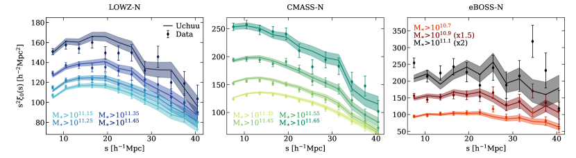
((a)) Monopole moment of the 2PCF.

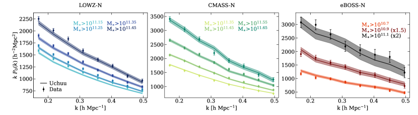
((b)) Monopole moment of the power spectrum.

Figure 9: Measurements of the 2PCF (a) and the power spectrum (b) monopoles for different stellar mass thresholds in CMASS-N (left column), LOWZ-N (middle column), and eBOSS-N (right column). The various stellar mass thresholds are indicated by the colour scheme in the legend. For a better visualization of the eBOSS sample, we have multiplied the $10.9$ and $11.1$ stellar mass thresholds measurements by $1.5$ and $2$ respectively. Observational measurements are shown by data points. The solid lines show the mean derived from the Uchuu lightcones. Data error bars represent the standard deviation of our set of GLAM-Uchuu lightcones at 1-$\sigma$ level, while the shaded area for Uchuu represents the error on the mean, $\sigma/\sqrt{2}$. We measure the 2PCF monopole from s$=5$ to $45\,h^{-1}\mathrm{Mpc}$ in $5\,h^{-1}\mathrm{Mpc}$ bins, and the power spectrum monopole from $\mathrm{k}=0.15$ to $0.5\,h\mathrm{Mpc}^{-1}$ in $0.05\,h\mathrm{Mpc}^{-1}$ bins.

We now investigate the completeness of the observed galaxy populations by analysing the dependence of the 2PCF and power spectrum monopoles on stellar mass. The results are shown in Fig. 9, where we observe that, for both the LOWZ and CMASS samples, a significant overlap exists between the observed data and the mean values obtained from the Uchuu lightcones across all the stellar mass thresholds. In agreement with previous studies (see Maraston et al., 2013), these results indicate that the LRG population in both BOSS samples is complete at the massive end. We conclude that the complete SMF assumed in the SHAM method for BOSS accurately describes the real galaxy populations.

For the eBOSS sample, consistent with results from Comparat et al. (2017), we consider an incomplete population of galaxies when generating the Uchuu-eBOSS lightcones. This is achieved by using a complete SMF that goes exceeds the SMF estimated from the data (see Section 4.1). Similar to the other samples, our goal is to assess whether the clustering as a function of stellar mass in Uchuu lightcones agrees with that estimated from the observed data. The results shown in the right panel of Fig. 9 demonstrate the accuracy of the method adopted in this work for modelling the incomplete eBOSS galaxy population. Despite the noise inherent to a low population statistic, there is a good agreement between the data and Uchuu, both samples presenting the same trend with stellar mass.

It is important to note that the eBOSS galaxy mass information was extracted from the Comparat et al. (2017) eBOSS catalog, which does not share the exact same footprint or n(z) as the public eBOSS data and Uchuu lightcones. Additionally, Comparat et al. (2017) does not provide its own random catalog, leading us to use the public random catalog for analysing the 2PCF. Again, this catalog does not present the same footprint and n(z). All these differences may introduce errors and discrepancies in the statistics. To mitigate these effects when computing the 2PCF for different stellar mass thresholds, we have selected galaxies from the Comparat et al. (2017) catalog that satisfy $\mathrm{DEC}>42\,\mathrm{deg}$ and $\mathrm{RA}<225\,\mathrm{deg}$. This subset aligns more closely with the footprint and n(z) of public data, as well as the random catalog. We do implement this filtering in the Uchuu-eBOSS lightcones as well.

6.1.3 Large-scale bias predictions

Sample	$z_{\mathrm{med}}$	$b^{\mathrm{data}}$	$b^{\mathrm{Uchuu}}$
LOWZ-N	$0.32$	$1.87\pm 0.03$	$1.87\pm 0.02$
CMASS-N	$0.57$	$1.99\pm 0.02$	$2.00\pm 0.02$
eBOSS-N	$0.70$	$2.10\pm 0.03$	$2.08\pm 0.02$

Table 5: Bias factors of the BOSS and eBOSS samples. The first and second columns give the sample name and its corresponding median redshift. The last two columns give the large-scale bias factors measured from the 2PCF monopole for both the observations and Uchuu lightcones. These bias factors have been obtained as the mean value of $b(\mathrm{s})$ within the range of $15$ to $30\,h^{-1}\mathrm{Mpc}$.

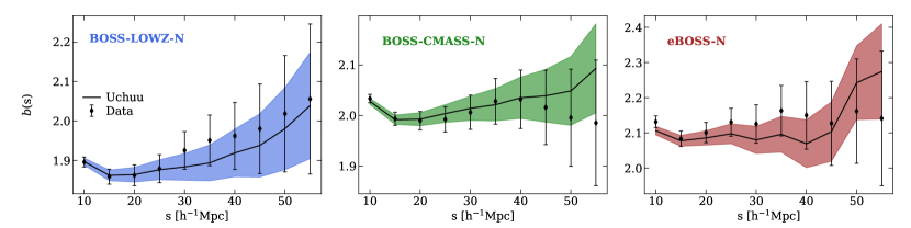
Figure 10: Measurements of the galaxy bias at the median redshift of the CMASS-N (left panel), LOWZ-N (middle panel) and eBOSS-N (right panel) samples. For details on the bias estimation see the text. In the case of the observations, the dark matter clustering is assumed to be the same as that in the Uchuu simulation. Observed data measurements are represented by points. The solid lines show the mean bias derived from the Uchuu lightcones for each of the samples. Data error bars represent the standard deviation of our set of GLAM-Uchuu lightcones at the 1-$\sigma$ level, and the shaded area corresponding to Uchuu indicates the error on the mean, $\sigma/\sqrt{2}$.

In Fig. 10, we study the galaxy bias, $b(\mathrm{s})$, through our theoretical predictions of the 2PCF monopole. We then proceed to compare these predictions with observed data. For each of the three studied samples, the large-scale bias at their respective median redshift, $z_{\mathrm{med}}$, is derived by solving the equation below, which gives a simple linear perturbation theory prediction of the RSD, which should be applicable on large scales (see Kaiser, 1987; Hamilton, 1998):

$$\xi_{0}(\mathrm{s})=b(\mathrm{s})^{2}\left(1+\frac{2}{3}\beta+\frac{1}{5}\beta^{2}\right)\xi_{\mathrm{lin}}(\mathrm{s}).$$ (11)

In the equation, we have $\beta=\Omega_{\mathrm{m},z_{\mathrm{med}}}^{0.55}/b(\mathrm{s})$, where $\xi_{0}(\mathrm{s})$ represents the measured 2PCF monopole (derived from data and lightcones in each case), and $\xi_{\mathrm{lin}}(\mathrm{s})$ correspond to the dark matter linear 2PCF from the Uchuu simulation at $z_{\mathrm{med}}$.

Our Uchuu BOSS/eBOSS lightcones reproduce the $b(\mathrm{s})$ values from observed data within the uncertainties. The BOSS/eBOSS bias factors, $b$, from both observed data and Uchuu lightcones, are presented in Table 5. The bias factors have been obtained as the mean value of $b(\mathrm{s})$ measured between $15$ and $30\,h^{-1}\mathrm{Mpc}$. This table clearly shows how the bias increases with the median redshift of the sample. This is in agreement with the results reported in Zhou et al. (2021), where a similar behaviour was observed when examining the evolution of large-scale bias with redshift for a DESI-type LRG population selected from the Legacy Survey imaging dataset (Dey et al., 2019).

6.1.4 Performance of Uchuu-COMB LRG lightcones

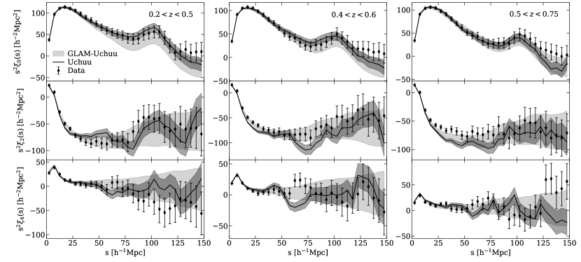
((a)) Large scale.

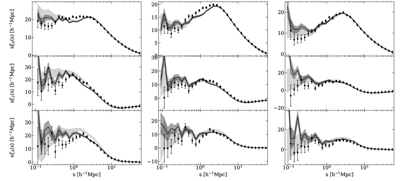
((b)) Small scale.

Figure 11: Measurements of the monopole, quadrupole and hexadecapole moments of the 2PCF for the COMB-N$+$S sample in three redshift ranges of interest: $0.2<z<0.5$ (left column), $0.4<z<0.6$ (middle column) and $0.5<z<0.75$ (right column). Observed data measurements are represented as data points. The solid line show the mean 2PCF derived from the Uchuu. We additionally show the standard deviation of GLAM-Uchuu around its mean in a light shaded area. Data error bars represent the standard deviation of our set of GLAM-Uchuu lightcones, 1-$\sigma$, while the dark shaded area for Uchuu is the error on the mean, $\sigma/\sqrt{2}$. Panel (a) shows the 2PCF measurements from $0$ to $150\,h^{-1}\mathrm{Mpc}$ in $5\,h^{-1}\mathrm{Mpc}$ bins, while panel (b) shows results up to $60\,h^{-1}\mathrm{Mpc}$ using equally-spaced logarithmic bins.

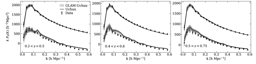
Figure 12: Measurements of the power spectrum monopole (upper curve) and quadrupole (lower curve) for the COMB-N$+$S sample in three redshift ranges of interest: $0.2<z<0.5$ (left panel), $0.4<z<0.6$ (middle panel) and $0.5<z<0.75$ (right panel). Observed data measurements are represented by data points. The solid line show the mean power spectrum derived from the Uchuu. We additionally show the standard deviation of GLAM-Uchuu around its mean in a light shaded area. Data error bars represent the standard deviation of our set of GLAM-Uchuu lightcones, 1-$\sigma$, while the dark shaded area for Uchuu is the error on the mean, $\sigma/\sqrt{2}$. The power spectrum is measured from $\mathrm{k}=0.005$ to $0.6\,h\mathrm{Mpc}^{-1}$ in bins of $0.03\,h\mathrm{Mpc}^{-1}$.

Finally, we assess the ability of our Uchuu-COMB lightcones to reproduce the observed BOSS clustering statistics in both hemispheres, N$+$S, as well as the clustering evolution with redshift. The monopole, quadrupole and hexadecapole moments of the 2PCF measurements are shown in Fig. 11 for both the observed data and mean Uchuu measurements. We additionally show the GLAM-Uchuu-COMB measurements with a light shaded area to demonstrate their behavior and to elucidate the source of potential discrepancies between Uchuu and the data. From left to right, the panels show the redshift intervals over which the 2PCF has been measured: $0.2<z<0.5$, $0.4<z<0.6$, and $0.5<z<0.75$. Correspondingly, we present the power spectrum monopole and quadrupole measurements from $\mathrm{k}=0.005$ to $0.6\,h\mathrm{Mpc}^{-1}$ in Fig. 12.

As anticipated, our Uchuu lightcones are able to fully reproduce, with high accuracy, the clustering evolution observed in the BOSS N$+$S data measurements. Residuals from the 2PCF monopole between the CMASS-N fibre collision scale, $4.2\,h^{-1}\mathrm{Mpc}$, and $25\,h^{-1}\mathrm{Mpc}$ ($100\,h^{-1}\mathrm{Mpc}$) exhibit values below $0.9\%$ ($8\%$) for $0.2<z<0.5$ sample, less than $1.5\%$ ($15\%$) for $0.4<z<0.6$ sample, and under $0.9\%$ ($10\%$) for $0.5<z<0.75$ sample. Regarding the power spectrum monopole between $k>0.03$ and $k<0.6\,h\mathrm{Mpc}^{-1}$, the residuals remain within $2.6,4.5,3.4\%$ for the three samples (left to right). We interpret the discrepancies in the 2PCF and power spectrum multipoles as arising from the same reasons as discussed in Section 6.1.1. Furthermore, the findings from GLAM-Uchuu validate that certain discrepancies between Uchuu and the data can be ascribed to statistical fluctuations. Our results are in agreement with previous works, both in configuration (see Chuang et al., 2017) and Fourier space (see Beutler et al., 2017).

The results presented in this section allow us to reach the conclusion that our theoretical predictions, based on the standard Planck cosmology model and built by generating lightcones from the Uchuu simulation, exhibit a remarkable ability to reproduce, with a high accuracy, the observed data across all studied samples: LOWZ, CMASS, COMB, and eBOSS, spanning both for Northern and Southern hemispheres. This reaffirms the high quality of the Uchuu simulation and highlights the reliability of our methodology. Notably, our approach relies on just one free parameter, the scatter $\sigma_{\mathrm{SHAM}}$, and covers various aspects, including adopting a complete SMF in the SHAM process and addressing the treatment of galaxy population incompleteness and fibre collision systematics.

6.2 Covariance errors from GLAM-Uchuu lightcones

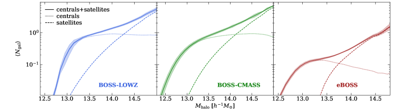
Figure 13: The HOD measured in the LOWZ (left panel), CMASS (middle panel) and eBOSS (right panel) samples, as determined from the mean of the Uchuu galaxy cubic boxes. The solid lines represent the combined HOD of centrals and satellites, while the dotted and dashed lines show the mean halo occupancy for centrals and satellites, respectively. The shaded area shows the standard deviation computed using 630 GLAM-Uchuu lightcones.

As described in Section 5.1, we populate the GLAM halos with galaxies using the HOD method. This statistic is obtained from the Uchuu galaxy cubic boxes and is shown in Fig. 13. By construction, the GLAM-Uchuu HOD agrees with that of the high-resolution Uchuu simulation. The forms of the HOD we recover are consistent with those found in previous BOSS and eBOSS LRG HOD studies (e.g. Nuza et al., 2013; Alam et al., 2020).

In this section, we analyze the covariance errors obtained from the GLAM-Uchuu covariance lightcones and present a comparison of these results with MD-Patchy and EZmock. For this analysis, we focus on the CMASS- and eBOSS-N samples, as the southern hemisphere samples have considerably smaller effective areas compared to the northern ones. Additionally, the LOWZ and COMB samples have significant discontinuities in their footprints.

For a fair comparison with GLAM-Uchuu, from the $2048$ MD-Patchy lightcones available, we have (randomly) selected 630 of those lightcones for the analyses carried out in this section. The same with EZmock: out of the $1000$ available, we have selected only 630.

6.2.1 Covariances in configuration space

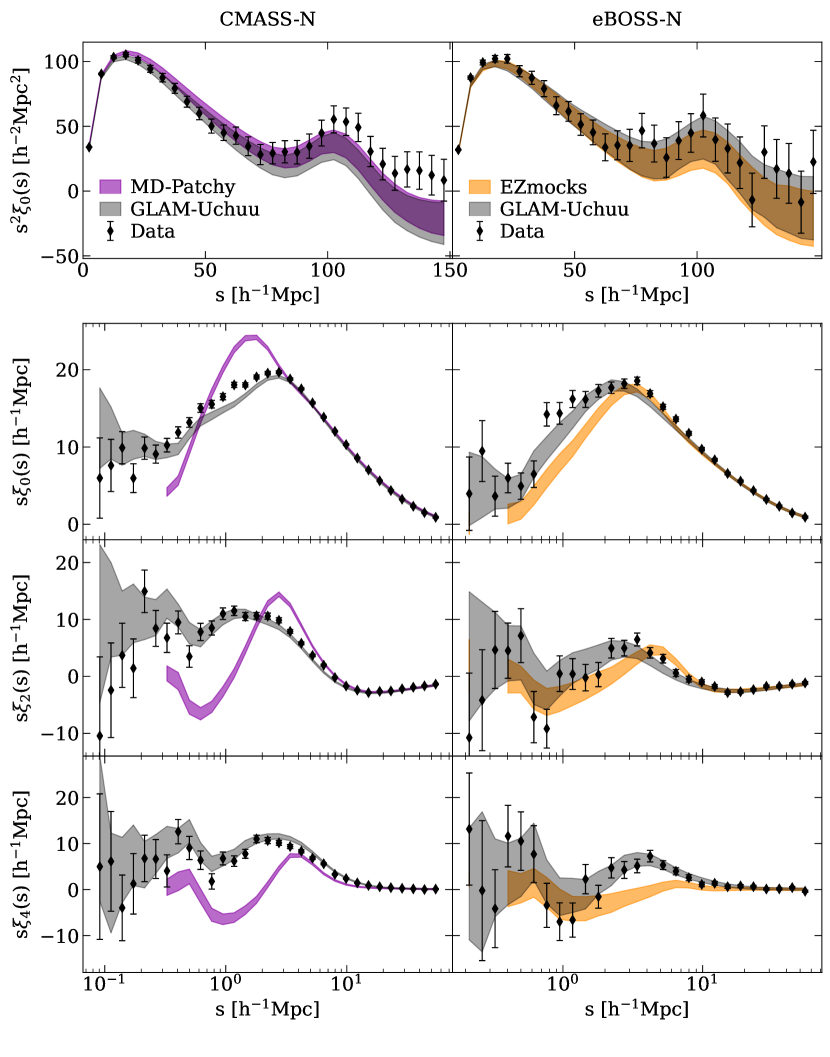
Figure 14: Measurements of the 2PCF monopole, quadrupole and hexadecapole moments for CMASS-N (left column) and eBOSS-N (right column). The shaded regions represent the standard deviation around its mean for GLAM-Uchuu (in black), MD-Patchy (purple, left column), and EZmock (orange, right column). The points with error bars show the measurements from the observed data, where the errors correspond to the 1-$\sigma$ scatter derived from GLAM-Uchuu lightcones. The upper panels show the 2PCF measurements from $0$ to $150\,h^{-1}\mathrm{Mpc}$ in $5\,h^{-1}\mathrm{Mpc}$ bins. The lower panels show the smaller scales up to $60\,h^{-1}\mathrm{Mpc}$ in equally-spaced logarithmic bins. It is evident that the MD-patchy and EZmock results exhibit significant discrepancies with the data between $0.1$ to $30\,h^{-1}\mathrm{Mpc}$, further emphasizing the need for generating the GLAM-Uchuu lightcones.

We compare the mean 2PCF multipole moments measured from the GLAM-Uchuu runs, along with those from MD-patchy and EZmock, in Fig. 14. The left column shows the analysis for the CMASS-N sample, while the right column corresponds to the eBOSS-N sample. Overall, GLAM-Uchuu accurately reproduces the observed CMASS-N and eBOSS-N data statistics across all studied multipoles and scales. However, when examining the results of MD-patchy and EZmock, it becomes evident that the their multipole moments exhibit strange features and discrepancies on scales below $20\,h^{-1}\mathrm{Mpc}$. The CMASS-N study also reveals that the resolution of GLAM-Uchuu lightcones is better than that of MD-patchy and EZmock, reaching down to scales of $0.1\,h^{-1}\mathrm{Mpc}$, in comparison to $0.3\,h^{-1}\mathrm{Mpc}$ and $0.4\,h^{-1}\mathrm{Mpc}$ for the other lightcones.

Furthermore, the behaviour observed in GLAM-Uchuu provides confirmation that some variations observed in earlier Uchuu multipole moments can be attributed to statistical fluctuations (Section 6.1.1), as these discrepancies diminish as the number of lightcones increases. For scales below $60\,h^{-1}\mathrm{Mpc}$, the 2PCF multipoles of GLAM remain within 1-$\sigma$ of the data for both BOSS and eBOSS, while Uchuu fluctuates between 1 and 2-$\sigma$ (see Fig. 5 (b)). The better improvement of the quadrupole and hexadecapole measurements as the number of lightcones increases in comparison to the monopole could potentially be associated with volumetric effects and harmonic modes within the data. The $\ell=2$ and $\ell=4$ moments might exhibit higher sensitivity to fluctuations arising from the geometric characteristics and configuration of the observed volume. By augmenting the quantity of lightcones and subsequent averaging, certain aspects of these influences might be alleviated.

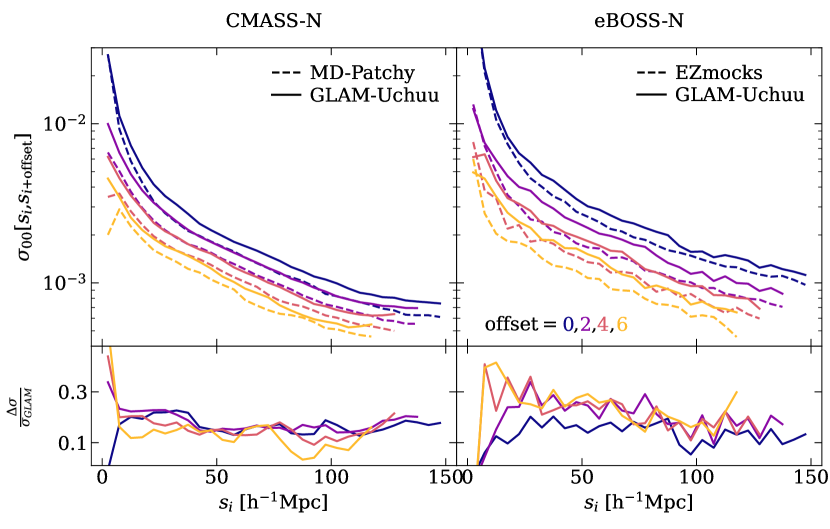
((a)) Covariance matrix diagonals.

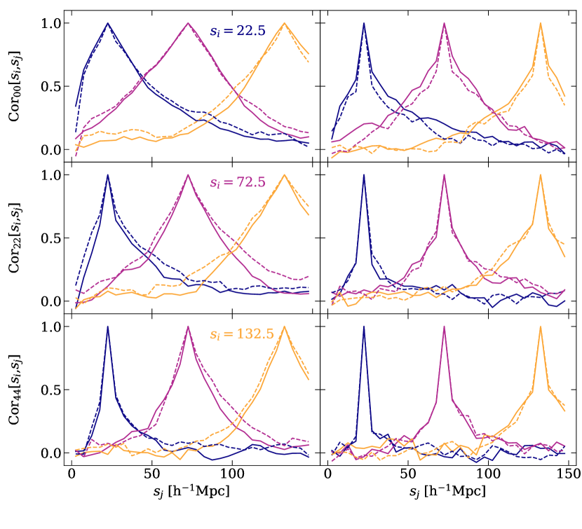
((b)) Correlation matrix rows.

Figure 15: Panel (a): Comparison between GLAM-Uchuu (solid line, both columns), MD-Patchy (dashed line, left column), and EZmock (dashed line, right column) covariance matrices of the 2PCF monopole, $\xi_{0}(\mathrm{s})$, for CMASS-N and eBOSS-N (left and right columns, respectively). Different colours represent distinct terms of the covariance matrices: diagonal term in blue and second, fourth and sixth off-diagonal terms in purple, pink, and orange respectively. The bottom panel shows the residuals between covariances. Panel (b): Cross-sections through the GLAM-Uchuu (solid lines), MD-Patchy (dashed line, left column), and EZmock (dashed line, right column) correlation matrices of the monopole, quadrupole and hexadecapole ($\ell=0,2,4$) moments of the 2PCF for CMASS-N and eBOSS-N (left and right columns respectively). Different colours represent distinct $\mathrm{s}_{i}$ values in units of $\,h^{-1}\mathrm{Mpc}$: $\mathrm{s}_{i}=22.5,72.5$ and $132.5$ in purple, pink, and yellow respectively.

The covariance matrix of the 2PCF multipoles, $\xi_{\ell}(s)$, can be estimated as follows:

$$\begin{split}\mathrm{Cov}_{\ell\ell^{\prime}}[s_{i},s_{j}]&=\\ &\frac{\mathcal{C}}{N_{\mathrm{m}}-1}\sum_{p}^{N_{\mathrm{m}}}\left[\xi_{\ell}^{p}(s_{i})-\overline{\xi}_{\ell}(s_{i})\right]\left[\xi_{\ell^{\prime}}^{p}(s_{j})-\overline{\xi}_{\ell^{\prime}}(s_{j})\right],\end{split}$$ (12)

where $N_{\mathrm{m}}$ is the number of lightcones, $\xi_{\ell}^{p}$ indicates the $l$-order 2PCF multipole of the $p$-th lightcone, and $\overline{\xi}_{\ell}$ denotes the mean 2PCF multipole of all the lightcones. The term $\mathcal{C}$ takes into account the dependence of $\mathrm{Cov}[s_{i},s_{j}]$ on the simulation box size (Klypin & Prada, 2018). When the effective volume of the observed sample, $V_{\mathrm{eff}}$, is smaller than that of the simulation volume, $V_{\mathrm{sim}}$, we have $\mathcal{C}=1$. However, when $V_{\mathrm{eff}}>V_{\mathrm{sim}}$, we must scale the covariance matrix by their volume ratio, i.e., $\mathcal{C}=V_{\mathrm{sim}}/V_{\mathrm{eff}}$. Notably, $\mathcal{C}\neq 1$ only for the GLAM-Uchuu-CMASS-N covariance matrix, where $\mathcal{C}=1/1.28$.

In Fig. 15 (a), we provide a comparison of different elements of the 2PCF monopole covariance matrices studied in this work. In particular, we show the diagonal and second, fourth and sixth off-diagonal terms. In the left column, we compare the GLAM-Uchuu-N results and MD-Patchy-CMASS-N. The values of the GLAM-Uchuu covariance matrix are higher than those of MD-Patchy for all the slices, with a discrepancy between the two that varies with the distance between galaxies, $s$, typically decreasing as $s$ gets bigger. This discrepancy fluctuates within the range of $10-25\%$, as shown by the residuals in the bottom panel. We compare GLAM-Uchuu and EZmock for the eBOSS-N sample in the right column. The trend is the same: the values of the GLAM-Uchuu elements are higher than those of EZmock. The disagreement in this case is larger for some values of $s$, reaching up to $40\%$. Discrepancies within the $20\%$ range are anticipated in both cases, and only discrepancies above this value are considered relevant (see Appendix B). Differences above this percentage are due to the different predictions of each simulation.

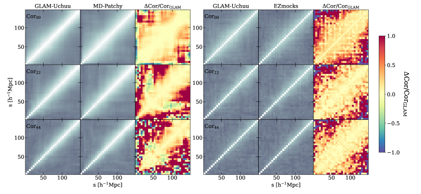
Figure 16: Left panel: Correlation matrices (Equation 13) of the 2PCF monopole, quadrupole and hexadecapole moments (first, second and third rows, respectively) obtained from GLAM-Uchuu (first column) and MD-Patchy (second column). The residuals, $r$, between GLAM-Uchuu and MD-patchy, are shown in the third column. Here, a positive value of $r$ indicates that the values of the GLAM-Uchuu correlation matrix are lower than those of MD-patchy, while $r<0$ means the opposite. Right panel: We examine the eBOSS-N sample covariances. The layout is identical to the left plot, but EZmock is used instead of MD-Patchy.

To further investigate the differences between the lightcones, one can also obtain the correlation matrices of the 2PCF multipoles:

$$\mathrm{Cor}_{\ell\ell^{\prime}}[\mathrm{s}_{i},\mathrm{s}_{j}]=\frac{\mathrm{Cov}_{\ell\ell^{\prime}}[\mathrm{s}_{i},\mathrm{s}_{j}]}{\sqrt{\mathrm{Cov}_{\ell\ell^{\prime}}[\mathrm{s}_{i},\mathrm{s}_{i}]\mathrm{Cov}_{\ell\ell^{\prime}}[\mathrm{s}_{j},\mathrm{s}_{j}]}}.$$ (13)

In Fig. 16, we report the derived correlation matrices for the monopole, quadrupole, and hexadecapole moments of the 2PCF. In the left plot, we show the correlation matrices obtained for the CMASS-N sample using GLAM-Uchuu, MD-Patchy, and the residuals between the two. The right plot follows the same, but for the eBOSS-N sample, replacing MD-Patchy with EZmock. In both cases, the residuals show distinct patterns in $\mathrm{Cor}_{00}$, $\mathrm{Cor}_{22}$ and $\mathrm{Cor}_{44}$.

To gain a deeper insight into the degree of correlation and the structure of these matrices, Fig. 15 (b) displays cross-sections through the covariance matrices that highlight the behaviour of their non-diagonal terms. We make a comparison for three separation values: $\mathrm{s}_{i}=22.5,72.5,132.5\,h^{-1}\mathrm{Mpc}$, as indicated by the colour scheme in the plot. In general, we observe a stronger correlation among bins located near the diagonal for the CMASS-N sample compared to the eBOSS-N, resulting in broader peaks in the former case. This correlation tends to weaker as we consider higher order multipoles. When examining individual cases, we notice that the off-diagonal elements of MD-Patchy display a higher level of correlation across all three multipoles when compared with GLAM-Uchuu. In comparison with EZmock, while GLAM-Uchuu presents more highly correlated off-diagonal elements for the monopole, it demonstrates similar results to EZmock for the quadrupole and hexadecapole.

6.2.2 Covariances in Fourier space

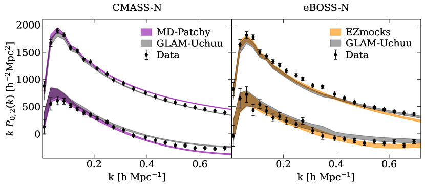
Figure 17: Measurements of the monopole (upper curve) and quadrupole (lower curve) moments of the power spectrum for the CMASS-N (left panel) and eBOSS-N (right panel) samples. The shaded regions represent the standard deviation around its mean for GLAM-Uchuu (in black), MD-Patchy (purple), and EZmock (orange) lightcone. Error bars represent the measurements taken from the observed data, where the errors are determined by the 1-$\sigma$ scatter derived from GLAM-Uchuu lightcones. We measure the power spectrum over the range $\mathrm{k}=0.005$ to $0.72\,h\mathrm{Mpc}^{-1}$, using $0.03\,h\mathrm{Mpc}^{-1}$ bins.

We analyze our GLAM lightcones in Fourier space using the same scheme and equations ($\xi_{\ell}(\mathrm{s})^{p}\rightarrow\mathrm{P}_{\ell}(\mathrm{k})^{p}$) as presented in the configuration space section.

First, we show the mean monopole and quadrupole moments of the power spectrum measured from GLAM-Uchuu, together with those from MD-Patchy and EZmock, in Fig. 17. The GLAM-Uchuu results are in good agreement with the observed CMASS-N and eBOSS-N clustering statistics for all the studied multipoles and scales. For k values above $0.4\,h\mathrm{Mpc}^{-1}$, the MD-Patchy and EZmock multipoles deviates from the data. This trend is consistent with that demonstrated in Fig. 14.

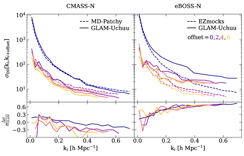
((a)) Covariance matrix diagonals.

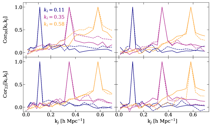
((b)) Correlation matrix rows.

Figure 18: Panel (a): Comparisons of the covariance matrices for the power spectrum monopole, $P_{0}(k)$, for CMASS-N and eBOSS-N (left and right columns respectively) between GLAM-Uchuu (solid line, both columns), MD-Patchy (dashed line, left column), and EZmock (dashed line, right column). Various colours represent different terms of the matrices: diagonal in blue, and second, fourth and sixth off-diagonal in purple, pink and orange respectively. The bottom panel shows the residuals between covariances. Panel (b): Slices through the correlation matrices of the power spectrum monopole and quadrupole for CMASS-N and eBOSS-N (left and right columns respectively) from GLAM-Uchuu (solid lines), MD-Patchy (dashed line, left column), and EZmock (dashed line, right column). Different colours correspond to distinct $\mathrm{k}_{i}$ values in units of $\,h\mathrm{Mpc}^{-1}$: $\mathrm{k}_{i}=0.11,0.35$ and $0.58$ in purple, pink, and yellow respectively.

Next, in Fig. 18 (a), we present the diagonal and second, fourth and sixth off-diagonal terms of the power spectrum monopole covariance matrices. In the left column, we compare GLAM-Uchuu and MD-Patchy for the CMASS-N sample, while the right column compares GLAM-Uchuu and EZmock for the eBOSS-N sample. The diagonal values of GLAM-Uchuu are slightly higher than those of MD-Patchy for low k values. However, this trend inverts for $\mathrm{k}\gtrsim 0.25\,h\mathrm{Mpc}^{-1}$. When comparing with EZmock, GLAM-Uchuu slices are higher at all scales, with a discrepancy between the two that increases with $\mathrm{k}_{i}$, reaching values above $60\%$ for $\mathrm{k}_{i}\geq 0.3\,h\mathrm{Mpc}^{-1}$. As in configuration space analysis, discrepancies within $20\%$ are expected, with discrepancies above this value attributed to the distinct predictions of each simulation.

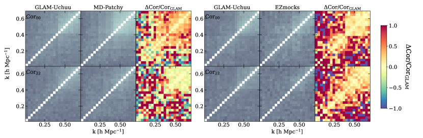
Figure 19: Left panel: Correlation matrices (as defined in Equation 13) of the power spectrum monopole and quadrupole (first and second rows) are obtained from GLAM-Uchuu (first column) and MD-Patchy (second column). The third column displays the residuals, $r$, between GLAM-Uchuu and MD-Patchy, where $r>0$ indicates that the values of the GLAM-Uchuu correlation matrix are lower than those of MD-Patchy, while $r<0$ indicates the opposite. Right panel: We conduct a similar study for the eBOSS-N sample. The layout is the same as the left plot, but EZmock is used instead of MD-Patchy.

We present the derived correlation matrices for the monopole and quadrupole moments of the power spectrum in Fig. 19. Following the same format as shown in Fig. 16, the left plot displays the correlation matrices obtained for the CMASS-N sample using GLAM-Uchuu and MD-Patchy. In the right plot, the eBOSS-N sample is analysed with EZmock instead of MD-Patchy. The residuals, $r$, are plotted in the third columns, showing again some patterns evident in both monopole and quadrupole moments. We show three cross-sections through these correlation matrices at $k_{i}=0.11,0.35,0.58\,h\mathrm{Mpc}^{-1}$ in Fig. 18 (b). In general, the correlation of the analysed cuts are very similar among GLAM-Uchuu, MD-Patchy and EZmock, particularly for the terms near the diagonal. For the bins located farther from the diagonal, noise becomes prominent and the signal amplitude is considerably low, posing challenges in determining clear trend. In the CMASS monopole case however, we clearly observe that MD-Patchy display a higher level of correlation than GLAM-Uchuu.

The analysis presented in this section confirms the reliability of the methodology applied in generating the GLAM-Uchuu covariance lightcones, as the accurately reproduce the clustering measurements from observations. Comparisons of the GLAM-Uchuu lightcones with the results from MD-Patchy and EZmock prove insightful. These approximate approaches exhibit peculiar behaviors in the multipole moments of the 2PCF. This clearly demonstrates the advantage of using $N$-body simulations over less accurate methods. We have verified that the diagonal elements of the GLAM-Uchuu covariance matrices surpass, in general, those obtained from MD-Patchy and EZmock. Consequently, the errors we estimate for the observed 2PCFs and power spectra are larger than previously assumed. However, it is important to remember that discrepancies within $20\%$ in the error estimation are anticipated. Only discrepancies above this value are considered relevant as they are, presumably, due to the different predictions of each simulation. The finding of discrepancies greater than this value subsequently leads to increased uncertainties in cosmological constraints derived from the BOSS and eBOSS data using MD-patchy or EZmock covariances, including those related to the BAO distance estimates and the estimation of cosmological parameters (see Alam et al., 2015, 2021, and references therein), as well as those to unveiling primordial non-Gaussianity (see Beutler et al., 2017; Merz et al., 2021; Mueller et al., 2022). Certain works that also employed MD-patchy or EZmock covariance matrices have reported tensions in the inferred value of $\sigma_{8}$ when compared with Planck measurements (see Wadekar et al., 2020; Chen et al., 2022; Kobayashi et al., 2022). This tension could potentially be mitigated or even disappear with larger uncertainties incorporated into the estimated parameters.

6.3 Performance with other cosmologies

Up to this point, we have demonstrated that our Uchuu clustering model, based on the standard Planck cosmology, is capable of accurately reproducing the observed clustering data while considering the relevant uncertainties. However, it is interesting to assess the performance of other cosmological models. For this purpose, we make use use our GLAM simulations runs for different cosmologies as presented in Section 3.2. These models are summarized in Table 2: GLAM-PMILL, GLAM-PMILLnoBAO and GLAM-Abacus. We note that their cosmological parameters are not considerably different from the Planck15 cosmology adopted for Uchuu. These newly generated lightcones follow the same process as the GLAM-Uchuu lightcones, as described in Section 5. It is worth highlighting that, regardless of the specific cosmology, galaxies are populated in all GLAM halo cubic boxes using the HODs obtained from the Uchuu galaxy boxes, which are based on the PL15 cosmology. Given the minor difference among the various explored cosmological parameters, creating distinct HODs for each cosmology would marginally improve the results while adding considerable additional complexity.

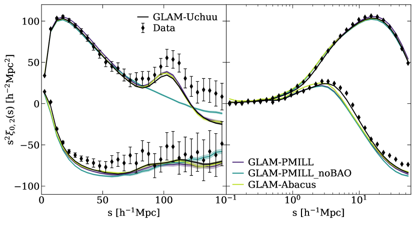
Figure 20: Measurements of the monopole and quadrupole moments of the 2PCF for the CMASS-N using different sets of GLAM simulations (see Table 2). The mean 2PCF derived from the GLAM-PMILL lightcones is represented by solid purple lines, GLAM-PMILLnoBAO in blue, GLAM-Abacus in green, and GLAM-Uchuuin black. The shaded regions represent the errors of the mean, estimated from the diagonal components of their respective covariance matrices. Data from observations are shown as points with error bars, where these indicate the 1-$\sigma$ errors estimated using the GLAM-Uchuu lightcones. The 2PCF measurements are performed from $0$ to $150\,h^{-1}\mathrm{Mpc}$ in $5\,h^{-1}\mathrm{Mpc}$ bins (left plot), and up to $60\,h^{-1}\mathrm{Mpc}$ in equally-spaced logarithmic bins (right plot).

The impact of the different cosmologies on the large-scale distribution of galaxies is shown in Fig. 20, where the mean monopole and quadrupole moments of the 2PCF obtained from the GLAM-PMILL, GLAM-PMILLnoBAO, and GLAM-Abacus lightcones for the CMASS-N sample. Additionally, results from observed data and theoretical predictions determined from the mean of the GLAM-Uchuu lightcones are shown for reference. In general, with the exception of GLAM-PMILLnoBAO, all GLAM lightcones effectively reproduce the observational measurements. The absence of the BAO feature in the GLAM-PMILLnoBAO monopole allow us, along with its BAO GLAM-PMILL counterpart, to assess the statistical significance of the BAO detection. Based on the analyzed measurements and and their associated uncertainties in this study, we cannot distinguish between the presence or absence of massive neutrinos. Although we achieve better results with GLAM-Uchuu (residuals below $3\%$ up to $50\,h^{-1}\mathrm{Mpc}$) compared to GLAM-Abacus, which includes the effect of massive neutrinos, resulting in residuals of $4\%$, both models are capable of reasonably reproducing the observed data within the errors.

7 Conclusions

We have generated LRG lightcones for the BOSS-LOWZ, -CMASS, -COMB and eBOSS samples, all based on the Planck cosmology. Specifically, we have created $16$ Uchuu lightcones, employing the SHAM technique to populate Uchuu (sub)halos with LRG galaxies. Additionally, we have produced 5,040 GLAM-Uchuu lightcones for estimating covariance errors using the HOD method. Furthermore, we created 800 supplementary lightcones using slightly different cosmologies than Planck 2015: GLAM-PMILL and -PMILLnoBAO, which adopt the cosmology of the Planck Millennium simulation (with and without BAO; Baugh et al. 2019), and GLAM-Abacus, which adopts the abacus$\_$cosm000 cosmology from the AbacusSummit $N$-body simulation suite (Maksimova et al., 2021). The methodology utilized in constructing all these lightcones ensures their ability to faithfully reproduce the observed evolution of galaxy clustering with redshift and stellar mass, in both configuration and Fourier space.

Throughout this study, we have studied various aspects of the LRG clustering signal. Firstly, we assess the capability of our theoretical predictions, derived from the Planck cosmology using our Uchuu LRG lightcones, in reproducing the BOSS and eBOSS data. The main results are summarised as follows:

1. We analyze galaxy clustering in both configuration and Fourier space for the LOWZ, CMASS, and eBOSS-N samples and compare them with our Uchuu lightcones. Overall, Uchuu accurately reproduces the correlation function and power spectrum measurements of the observed data. We find certain discrepancies on large scales, primary caused by cosmic variance and the substantial impact of observational systematics. On smaller scales, below $\sim 1\,h^{-1}\mathrm{Mpc}$, these deviations can be attributed to the non-application of PIP weights in our analysis. In configuration space, our findings indicate that the residuals of the 2PCF monopole remain within the range of $10\%$ ($15\%$ for eBOSS) up to $100\,h^{-1}\mathrm{Mpc}$ and fall below $2.5\%$ up to $25\,h^{-1}\mathrm{Mpc}$. Moving to Fourier space, we observe that the power spectrum monopole residuals between $k=0.03$ and $k=0.6\,h\mathrm{Mpc}^{-1}$ are below $12.5\%$ for eBOSS, and drop under $5\%$ and $4\%$ for LOWZ and CMASS, respectively.

2. From the clustering dependence with stellar mass, we can conclude that the observed LRG population in both BOSS samples is complete at the massive end. We also validate the accuracy of the method adopted in this work for modeling the incompleteness of the eBOSS galaxy population.

3. The scale-dependent galaxy bias of our Uchuu lightcones is measured and compared with that from observations, finding a good agreement between the two. Additionally, we observe an increase in the bias factor with redshift.

4. Finally, we check whether our theoretical predictions reproduce the observed evolution of clustering with redshift by analyzing the 2PCF and the power spectrum of the COMB sample in three redshift bins. In general, we find a good agreement between the Uchuu (and GLAM-Uchuu)lightcones and the observed data. We report 2PCF monopole residuals that remain under $1.5\%$ ($12\%$) within the range of $25\,h^{-1}\mathrm{Mpc}$ ($100\,h^{-1}\mathrm{Mpc}$), and within $4.5\%$ for monopole power spectrum between $k=0.03$ and $k=0.6$. Any potential discrepancies can be attributed to the same factors mentioned in (i).

We have also generated 630 GLAM-Uchuu lightcones for each of the BOSS and eBOSS samples, aimed at estimating covariance errors. We then compare these lightcones with the observational data, along with comparing their covariance and correlation matrices with those obtained in previous works. In our analyses of the 2PCF and power spectrum multipoles, we find that our GLAM-Uchuu covariance lightcones accurately reproduce the observational data. Strikingly, MD-Patchy and EZmock LRG lightcones display peculiar features in their multipoles that deviate from observations within $20\,h^{-1}\mathrm{Mpc}$ and for $\mathrm{k}>0.4\,h\mathrm{Mpc}^{-1}$. Moreover, due to its higher resolution inherent to $N$-body simulations, GLAM-Uchuu agrees with the data even on scales as small $0.1\,h^{-1}\mathrm{Mpc}$, in contrast to those approximate methods. In the covariance matrices (error estimation) comparison, discrepancies between GLAM-Uchuu and MD-Patchy remain, in general, within $20\%$. With EZmock these deviations reach values of up to $60\%$. However, discrepancies within $20\%$ are to be expected, with those above this value being attributed to the distinct predictions of each simulation. Regarding the correlation matrices, we notice that GLAM-Uchuu presents lower correlation compared to MD-Patchy, but similar to EZmock. These results not only confirm the reliability of the methodology applied to generate our GLAM-Uchuu covariance lightcones, but also highlight the importance of employing $N$-body simulations over approximate methods for accurately estimating covariance errors.

Finally, we explore the impact of cosmology on galaxy clustering using the various available GLAM runs. Our analysis reveals that it is not feasible to discern between a universe with or without massive neutrinos within the current BOSS/eBOSS uncertainties.

In conclusion, our theoretical predictions, based in the Planck cosmology and derived from the high-fidelity Uchuu lightcones, affirm both the accuracy of Planck in explaining observations of the in LSS BOSS/eBOSS surveys and the robustness of the Uchuu simulation. These findings have significant implications for the refinement of lightcone construction methodologies and the advancement of our understanding of clustering measurements. Moreover, we demonstrate that both MD-Patchy and EZmock LRG lightcones systematically underestimate uncertainties by $\approx 10-60\%$ compared to GLAM-Uchuu, which has significant implications for cosmological parameter inferences derived from BOSS and eBOSS.

A similar study, as presented here, can be expanded by using the Modify Gravity version of GLAM (MG-GLAM; see Hernández-Aguayo et al., 2022; Ruan et al., 2022) for the analyses of BOSS/eBOSS clustering, potentially revealing novel insights into the nature of gravity. In the near future, we are planning to generate Uchuu LRG lightcones for the first year of DESI data. We will then build their covariance matrices within the framework of GLAM-Uchuu, as presented in this paper. This effort will significantly enhance the precision of the cosmological analyses carried out using the DESI data.

Data Availability

The datasets included in this work consist of the following: $2~{}\mathrm{(lightcones)}\times 8~{}\mathrm{(samples)}$ Uchuu lightcones, the $630\times 8$ GLAM-Uchuu lightcones, the $100\times 8$ GLAM-PMILL, GLAM-PMILLnoBAO and GLAM-Abacus lightcones, along with the BOSS and eBOSS catalogues. These datasets will be made publicly available at http://www.skiesanduniverses.org/Simulations/Uchuu/. A comprehensive list and brief description of the catalogue columns can be found in Appendix A.

Appendix A Content of the public catalogues

Below is a list of the columns of each data set, along with a short description.

A.1 Uchuu lightcones

Each Uchuu lightcone has the following columns:

• ra: right ascension (degrees).

• dec: declination (degrees).

• z_cos: cosmological redshift.

• z_obs: observed redshift (accounting for peculiar velocities).

• nz: number density of galaxies, n(z), at the redshift of the galaxy ($h^{3}\mathrm{Mpc}^{-3}$).

• logMstll: logarithm ($\log_{10}$) of the galaxy stellar mass (M_⊙).

• poly_id: healpix pixel ID containing the galaxy.

• poly_w: fibre-collision completeness in the healpix pixel containing the galaxy.

• w_cp: fibre collision correction weight (NNW).

• w_fkp: FKP weight.

In addition, the following columns describe the properties of the DM host (sub)halos of galaxies. These are taken from the original values in the Uchuu simulation halo catalogues:

• Mvir_all: mass enclosed within the virial overdensity, including unbound particles ($\,h^{-1}\mathrm{M_{\odot}}$).

• Rvir: virial radius ($\,h^{-1}\mathrm{kpc}$).

• rs: scale radius of a fitted NFW profile (comoving $\,h^{-1}\mathrm{kpc}$).

• Cvir: dark matter concentration within Rvir.

• Vpeak: peak value of $V_{\mathrm{max}}$ over the halo history (physical $\mathrm{km}\text{\,}{\mathrm{s}}^{-1}$).

• id: ID that identify each (sub)halo (unique in the whole simulation).

• pid: ID of the parent central halo for satellite halos, -1 for central halos.

• x, y, z: 3D position coordinates. The coordinate system of the Uchuu cubic box has been shifted so that the observer is at the origin, and there are periodic replications of the box (comoving $\,h^{-1}\mathrm{Mpc}$).

• vx, vy, vz: 3D velocity (physical $\,\mathrm{km\,s^{-1}}$).

• vrms: velocity dispersion (physical $\,\mathrm{km\,s^{-1}}$).

• vlos: velocity vector projected along line-of-sight, with the observer positioned at the origin ($\,\mathrm{km\,s^{-1}}$).

Random catalogues, containing $40$ times the number of galaxies of an individual catalogue, are also provided.

A.2 GLAM lightcones

Each GLAM lightcone has the following columns:

• gal_id: indicates whether the galaxy is central or a satellite (1 for centrals, 2 for satellites).

• ra

• dec

• z_cos

• z_obs

• nz

• logMstll

• poly_id

• poly_w

• w_cp

• w_fkp

In addition, the following columns describe the DM host halo (not subhalos) properties of galaxies, taken from the original values found in the GLAM simulation halo catalogues,

• Mtotal: halo virial mass ($\,h^{-1}\mathrm{M_{\odot}}$).

• Rvir

• rs

• x, y, z: 3D position coordinates. The coordinate system of the GLAM cubic box has been shifted so that the observer is at the origin, and there are periodic replications of the box (comoving $\,h^{-1}\mathrm{Mpc}$).

• vx, vy, vz

• vlos

Random catalogues, containing $30$ times the number of galaxies of an individual catalogue, are also provided.

A.3 BOSS and eBOSS data samples

In order to facilitate any analysis, we also make available the observed galaxy samples used is this work. The columns are as follows:

• RA: right ascension (degrees).

• DEC: declination (degrees).

• Z: measured redshift, including fibre collisions.

• NZ: number density of galaxies, n(z), at the redshift of the galaxy ($h^{3}\mathrm{Mpc}^{-3}$).

• WEIGHT_CP: fibre collision correction weight.

• WEIGHT_NOZ: redshift failures weight.

• WEIGHT_SYSTOT: total angular systematic weight.

• WEIGHT_FKP: FKP weight.

Random catalogues, containing $40$ times the number of galaxies of an individual catalogue, are also provided.

Appendix B Effect of box size and replication in covariance matrices

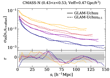
((a)) Test 1: Covariance for $0.43<z<0.53$

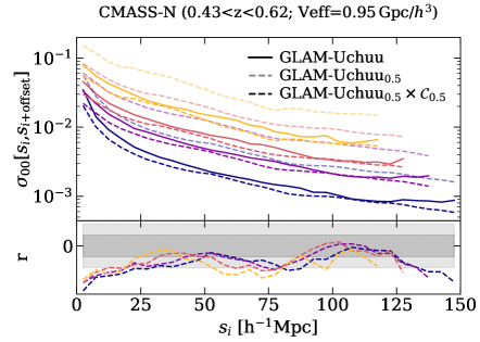
((b)) Test 2: Covariance for $0.43<z<0.62$

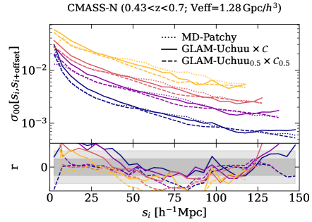
((c)) Test 3: Covariance for $0.43<z<0.7$

Figure 21: Comparison between CMASS-N covariance matrices of the 2PCF monopole for different redshift ranges. Different colours represent distinct terms of the covariance matrices: diagonal term in blue and second, fourth and sixth off-diagonal terms in purple, pink, and orange respectively. The light (dark) shaded area in the bottom panels represents residuals within $10\%$ ($20\%$). Panel (a): GLAM-Uchuu (solid line) and GLAM-Uchuu_0.5 (dashed line) covariances for $0.43<z<0.53$ ($V_{\mathrm{eff}}=0.47\,h^{-3}$Gpc). The bottom panel shows the residuals between covariances. Panel (b): GLAM-Uchuu (solid line), GLAM-Uchuu_0.5 (dashed line, lighter colour), and GLAM-Uchuu${}_{0.5}\,\mathrm{x}\,\mathcal{C}_{0.5}$ (dashed line, darker colour) covariances for $0.43<z<0.62$ ($V_{\mathrm{eff}}=0.95\,h^{-3}$Gpc). The bottom panel shows the residuals between GLAM-Uchuu and GLAM-Uchuu${}_{0.5}\,\mathrm{x}\,\mathcal{C}_{0.5}$ covariances. Panel (c): MD-patchy (dotted line), GLAM-Uchuu$\,\mathrm{x}\,\mathcal{C}$ (solid line), and GLAM-Uchuu${}_{0.5}\,\mathrm{x}\,\mathcal{C}_{0.5}$ (dashed line) for $0.43<z<0.7$ ($V_{\mathrm{eff}}=1.28\,h^{-3}$Gpc). We show the residuals between MD-patchy and GLAM-Uchuu$\,\mathrm{x}\,\mathcal{C}$ (GLAM-Uchuu${}_{0.5}\,\mathrm{x}\,\mathcal{C}_{0.5}$) with a solid (dashed) line in the bottom panel.

Throughout this study, there is a point where the reader may be concerned about our conclusions: the comparison between the covariance matrices of GLAM-Uchuu, MD-patchy, and EZmock (Section 6.2). One of our claims is that our estimated errors are up to $60\%$ higher than those previously reported with EZmock for the eBOSS sample. We also find discrepancies of around $20\%$ with MD-patchy. One might think that these differences in covariances are related to the different box sizes of the simulations: GLAM-Uchuu has a box size of $1\,h^{-1}\mathrm{Gpc}$, MD-patchy of $2.5\,h^{-1}\mathrm{Gpc}$, and EZmock of $6\,h^{-1}\mathrm{Gpc}$. Firstly, it is important to note that the GLAM-Uchuu box size might only impacts the CMASS-N covariance matrix. For all other studied samples, the observed effective volumes are smaller than the size of the GLAM-Uchuu boxes, and consequently the estimation of errors is not affected.

For the construction of CMASS-N GLAM-Uchuu lightcones, box replications are needed to cover the observed volume, $V_{\mathrm{eff}}=1.27\,h^{-3}$Gpc³, since this is larger than the GLAM-Uchuu box size. In this situation, it is expected that the covariance matrix may be affected. To address the effect that box replications have on covariance matrix, we have conducted a series of tests (all focused on the CMASS-N sample, see Figure 21). Firstly, we construct 100 new lightcones for this sample using GLAM-Uchuu boxes of $0.5\,h^{-1}$Gpc. These lightcones are referred to as GLAM-Uchuu_0.5 (distinct from GLAM-Uchuu, constructed with $1\,h^{-1}$Gpc boxes).

In an initial test (“test 1”), we analyze the covariance matrices of GLAM-Uchuu and GLAM-Uchuu_0.5 for the monopole between $0.43<z<0.53$. This redshift range results in an observed effective volume of $0.47\,h^{-3}$Gpc³. This volume is smaller than both box sizes, so their covariances should remain unaffected, and consequently, they should predict similar values. The results of this test are depicted in Figure 21 (a). Here, we observe that indeed the covariance of GLAM-Uchuu and GLAM-Uchuu_0.5 aligns, with residuals staying within the $20\%$ range.

Next (“test 2”), we re-evaluate the covariance matrices of GLAM-Uchuu and GLAM-Uchuu_0.5, this time between $0.43<z<0.62$. This redshift range yields an observed effective volume of $0.95\,h^{-3}$Gpc³, larger than the box size of GLAM-Uchuu_0.5, but smaller than that of GLAM-Uchuu. In this case, the covariance of GLAM-Uchuu_0.5 should be affected due to the need of box replications to cover the analysed redshift range. On the other hand, no replications are needed in the construction of GLAM-Uchuu lightcones, so its covariance should remain unaffected. The results of this test are illustrated in Figure 21 (b), revealing a difference in the covariance of GLAM-Uchuu and GLAM-Uchuu_0.5. To correct for the box size effect on covariance, we apply the correction presented in Equation 12: we multiply the covariance matrices of GLAM-Uchuu_0.5 by $\mathcal{C}_{0.5}=V_{\mathrm{sim}}/V_{\mathrm{eff}}=0.5^{3}/0.95$. The result of this operation is displayed in the plot with dark dashed lines (GLAM-Uchuu_0.5$\,\mathrm{x}\,\mathcal{C}_{0.5}$). After this correction, the covariance aligns with that of GLAM-Uchuu, with residuals once again staying within $20\%$.

In the third and final test (“test 3”), we analyze the covariance matrices in $0.43<z<0.7$, with an effective volume of $1.28\,h^{-3}$Gpc³. This effective volume is larger than the box size of both GLAM-Uchuu and GLAM-Uchuu_0.5, so it is expected that both covariances will be affected due to the need of replications to cover the analysed redshift range. Once again, we correct these covariances by multiplying by $\mathcal{C}=1/1.28$ (GLAM-Uchuu$\,\mathrm{x}\,\mathcal{C}$), and $\mathcal{C}_{0.5}=0.5^{3}/1.28$ (GLAM-Uchuu_0.5$\,\mathrm{x}\,\mathcal{C}_{0.5}$). The results are presented in Figure 21 (c), alongside the covariance of MD-patchy (box size of $2.5\,h^{-1}$Gpc). This plot demonstrates how the volume correction applied to GLAM-Uchuu and GLAM-Uchuu_0.5 lightcones corrects for the box size. Once again, residuals stay within the $20\%$ range.

After this study, we can draw several conclusions:

• Test 1 would be the equivalent scenario to the comparison between covariances of GLAM-Uchuu and EZmock for the eBOSS-N sample. The eBOSS-N sample has an effective volume of $0.26\,h^{-3}$Gpc³, smaller than both box sizes. Therefore, we anticipate that the covariances of both sets of lightcones will predict similar values (assuming a $20\%$ discrepancy). Differences above this percentage will be due to the different predictions of each simulation.

• According to tests 2 and 3, we reaffirm the validity of the correction applied to the covariance matrix of GLAM-Uchuu-CMASS-N to rectify the effect of box size and replication. Once the correction is applied, both sets of lightcones, GLAM-Uchuu and MD-patchy, should predict the same values. Again, any differences above $20\%$ will be due to the different predictions of each simulation.

References

- Ahumada et al. (2020) Ahumada R., et al., 2020, ApJS, 249, 3
- Alam et al. (2015) Alam S., et al., 2015, ApJS, 219, 12
- Alam et al. (2017) Alam S., et al., 2017, MNRAS, 470, 2617
- Alam et al. (2020) Alam S., Peacock J. A., Kraljic K., Ross A. J., Comparat J., 2020, MNRAS, 497, 581
- Alam et al. (2021) Alam S., et al., 2021, Phys. Rev. D, 103, 083533
- Aung et al. (2023) Aung H., et al., 2023, MNRAS, 519, 1648
- Barrera et al. (2022) Barrera M., et al., 2022, The MillenniumTNG Project: Semi-analytic galaxy formation models on the past lightcone (arXiv:2210.10419)
- Baugh et al. (2019) Baugh C. M., et al., 2019, MNRAS, 483, 4922
- Behroozi et al. (2010) Behroozi P. S., Conroy C., Wechsler R. H., 2010, ApJ, 717, 379
- Behroozi et al. (2013a) Behroozi P. S., Wechsler R. H., Wu H.-Y., 2013a, ApJ, 762, 109
- Behroozi et al. (2013b) Behroozi P. S., Wechsler R. H., Wu H.-Y., Busha M. T., Klypin A. A., Primack J. R., 2013b, ApJ, 763, 18
- Berlind & Weinberg (2002) Berlind A. A., Weinberg D. H., 2002, ApJ, 575, 587
- Beutler et al. (2017) Beutler F., et al., 2017, MNRAS, 464, 3409
- Bianchi & Percival (2017) Bianchi D., Percival W. J., 2017, MNRAS, 472, 1106
- Chaves-Montero et al. (2016) Chaves-Montero J., Angulo R. E., Schaye J., Schaller M., Crain R. A., Furlong M., Theuns T., 2016, MNRAS, 460, 3100
- Chen et al. (2022) Chen S.-F., Vlah Z., White M., 2022, J. Cosmology Astropart. Phys., 2022, 008
- Chuang et al. (2017) Chuang C.-H., et al., 2017, MNRAS, 471, 2370
- Cole et al. (2005) Cole S., et al., 2005, MNRAS, 362, 505
- Comparat et al. (2017) Comparat J., et al., 2017, Stellar population properties for 2 million galaxies from SDSS DR14 and DEEP2 DR4 from full spectral fitting, doi:10.48550/ARXIV.1711.06575, https://arxiv.org/abs/1711.06575
- Contreras et al. (2021) Contreras S., Angulo R. E., Zennaro M., 2021, MNRAS, 508, 175
- Contreras et al. (2023a) Contreras S., Angulo R. E., Chaves-Montero J., White S. D. M., Aricò G., 2023a, MNRAS, 520, 489
- Contreras et al. (2023b) Contreras S., et al., 2023b, MNRAS, 524, 2489
- DESI Collaboration et al. (2022) DESI Collaboration et al., 2022, AJ, 164, 207
- Davis & Peebles (1983) Davis M., Peebles P. J. E., 1983, ApJ, 267, 465
- Dawson et al. (2013) Dawson K. S., et al., 2013, AJ, 145, 10
- Dawson et al. (2016) Dawson K. S., et al., 2016, AJ, 151, 44
- Dey et al. (2019) Dey A., et al., 2019, AJ, 157, 168
- Dong-Páez et al. (2022) Dong-Páez C. A., et al., 2022, The Uchuu-SDSS galaxy lightcones: a clustering, RSD and BAO study (arXiv:2208.00540)
- Eisenstein et al. (2005) Eisenstein D. J., et al., 2005, ApJ, 633, 560
- Feldman et al. (1994) Feldman H. A., Kaiser N., Peacock J. A., 1994, ApJ, 426, 23
- Frenk et al. (1999) Frenk C. S., et al., 1999, ApJ, 525, 554
- Guo et al. (2012) Guo H., Zehavi I., Zheng Z., 2012, ApJ, 756, 127
- Guo et al. (2016) Guo H., et al., 2016, MNRAS, 459, 3040
- Hamilton (1998) Hamilton A. J. S., 1998, in Hamilton D., ed., Astrophysics and Space Science Library Vol. 231, The Evolving Universe. p. 185 (arXiv:astro-ph/9708102), doi:10.1007/978-94-011-4960-0_17
- Hand et al. (2017) Hand N., Li Y., Slepian Z., Seljak U., 2017, J. Cosmol. Astropart. Phys., 2017, 002
- Hayashi et al. (2003) Hayashi E., Navarro J. F., Taylor J. E., Stadel J., Quinn T., 2003, ApJ, 584, 541
- Hernández-Aguayo et al. (2021) Hernández-Aguayo C., Prada F., Baugh C. M., Klypin A., 2021, Monthly Notices of the Royal Astronomical Society, 503, 2318
- Hernández-Aguayo et al. (2022) Hernández-Aguayo C., Ruan C.-Z., Li B., Arnold C., Baugh C. M., Klypin A., Prada F., 2022, J. Cosmology Astropart. Phys., 2022, 048
- Hernández-Aguayo et al. (2023) Hernández-Aguayo C., et al., 2023, Mon. Not. Roy. Astron. Soc., 524, 2556
- Huterer et al. (2013) Huterer D., Cunha C. E., Fang W., 2013, Monthly Notices of the Royal Astronomical Society, 432, 2945
- Ishiyama et al. (2009) Ishiyama T., Fukushige T., Makino J., 2009, PASJ, 61, 1319
- Ishiyama et al. (2012) Ishiyama T., Nitadori K., Makino J., 2012, arXiv e-prints, p. arXiv:1211.4406
- Ishiyama et al. (2021) Ishiyama T., et al., 2021, MNRAS, 506, 4210
- Kaiser (1987) Kaiser N., 1987, MNRAS, 227, 1
- Kitaura et al. (2014) Kitaura F. S., Yepes G., Prada F., 2014, MNRAS, 439, L21
- Kitaura et al. (2016) Kitaura F.-S., et al., 2016, MNRAS, 456, 4156
- Kitzbichler & White (2007) Kitzbichler M. G., White S. D. M., 2007, MNRAS, 376, 2
- Klypin & Prada (2018) Klypin A., Prada F., 2018, MNRAS, 478, 4602
- Klypin et al. (2016) Klypin A., Yepes G., Gottlöber S., Prada F., Heß S., 2016, Monthly Notices of the Royal Astronomical Society, 457, 4340
- Kobayashi et al. (2022) Kobayashi Y., Nishimichi T., Takada M., Miyatake H., 2022, Phys. Rev. D, 105, 083517
- Kravtsov et al. (2004) Kravtsov A. V., Berlind A. A., Wechsler R. H., Klypin A. A., Gottlöber S., Allgood B., Primack J. R., 2004, ApJ, 609, 35
- Landy & Szalay (1993) Landy S. D., Szalay A. S., 1993, ApJ, 412, 64
- Maksimova et al. (2021) Maksimova N. A., Garrison L. H., Eisenstein D. J., Hadzhiyska B., Bose S., Satterthwaite T. P., 2021, Monthly Notices of the Royal Astronomical Society, 508, 4017
- Maraston et al. (2013) Maraston C., et al., 2013, MNRAS, 435, 2764
- Masaki et al. (2023) Masaki S., Kashino D., Ishikawa S., Lin Y.-T., 2023, MNRAS, 523, 5280
- Merson et al. (2019) Merson A., Smith A., Benson A., Wang Y., Baugh C., 2019, MNRAS, 486, 5737
- Merz et al. (2021) Merz G., et al., 2021, MNRAS, 506, 2503
- Mohammad et al. (2020) Mohammad F. G., et al., 2020, MNRAS, 498, 128
- Moustakas et al. (2013) Moustakas J., et al., 2013, ApJ, 767, 50
- Mueller et al. (2022) Mueller E.-M., et al., 2022, MNRAS, 514, 3396
- Norberg et al. (2009) Norberg P., Baugh C. M., Gaztañaga E., Croton D. J., 2009, MNRAS, 396, 19
- Nuza et al. (2013) Nuza S. E., et al., 2013, Monthly Notices of the Royal Astronomical Society, 432, 743
- Oogi et al. (2022) Oogi T., et al., 2022, arXiv e-prints, p. arXiv:2207.14689
- Pakmor et al. (2023) Pakmor R., et al., 2023, Mon. Not. Roy. Astron. Soc., 524, 2539
- Peacock & Smith (2000) Peacock J. A., Smith R. E., 2000, MNRAS, 318, 1144
- Peacock et al. (2001) Peacock J. A., et al., 2001, Nature, 410, 169
- Percival et al. (2004) Percival W. J., Verde L., Peacock J. A., 2004, MNRAS, 347, 645
- Planck Collaboration et al. (2014) Planck Collaboration et al., 2014, A&A, 571, A16
- Planck Collaboration et al. (2016) Planck Collaboration et al., 2016, A&A, 594, A13
- Prada et al. (2023) Prada F., Behroozi P., Ishiyama T., Klypin A., Pérez E., 2023, arXiv e-prints, p. arXiv:2304.11911
- Prakash et al. (2016) Prakash A., et al., 2016, ApJS, 224, 34
- Reddick et al. (2013) Reddick R. M., Wechsler R. H., Tinker J. L., Behroozi P. S., 2013, ApJ, 771, 30
- Reid et al. (2015) Reid B., et al., 2015, SDSS-III Baryon Oscillation Spectroscopic Survey Data Release 12: galaxy target selection and large scale structure catalogues, doi:10.48550/ARXIV.1509.06529, https://arxiv.org/abs/1509.06529
- Rodríguez-Torres et al. (2016) Rodríguez-Torres S. A., et al., 2016, MNRAS, 460, 1173
- Ross et al. (2017) Ross A. J., et al., 2017, MNRAS, 464, 1168
- Ross et al. (2020) Ross A. J., et al., 2020, MNRAS, 498, 2354
- Ruan et al. (2022) Ruan C.-Z., Hernández-Aguayo C., Li B., Arnold C., Baugh C. M., Klypin A., Prada F., 2022, J. Cosmology Astropart. Phys., 2022, 018
- Schaye et al. (2023) Schaye J., et al., 2023, arXiv e-prints, p. arXiv:2306.04024
- Sefusatti et al. (2016) Sefusatti E., Crocce M., Scoccimarro R., Couchman H. M. P., 2016, Mon. Not. R. Astro. Soc., 460, 3624
- Skibba et al. (2011) Skibba R. A., van den Bosch F. C., Yang X., More S., Mo H., Fontanot F., 2011, MNRAS, 410, 417
- Smith et al. (2017) Smith A., Cole S., Baugh C., Zheng Z., Angulo R., Norberg P., Zehavi I., 2017, MNRAS, 470, 4646
- Smith et al. (2022) Smith A., Cole S., Grove C., Norberg P., Zarrouk P., 2022, MNRAS, 516, 4529
- Springel (2005) Springel V., 2005, MNRAS, 364, 1105
- Stoppacher et al. (2019) Stoppacher D., et al., 2019, MNRAS, 486, 1316
- Trujillo-Gomez et al. (2011) Trujillo-Gomez S., Klypin A., Primack J., Romanowsky A. J., 2011, ApJ, 742, 16
- Vale & Ostriker (2006) Vale A., Ostriker J. P., 2006, MNRAS, 371, 1173
- Wadekar et al. (2020) Wadekar D., Ivanov M. M., Scoccimarro R., 2020, Phys. Rev. D, 102, 123521
- Wechsler et al. (2001) Wechsler R. H., Somerville R. S., Bullock J. S., Kolatt T. S., Primack J. R., Blumenthal G. R., Dekel A., 2001, Astrophys. J., 554, 85
- Yu et al. (2022) Yu J., et al., 2022, MNRAS, 516, 57
- Yu et al. (2023) Yu B., Seljak U., Li Y., Singh S., 2023, J. Cosmology Astropart. Phys., 2023, 057
- Zel’dovich (1970) Zel’dovich Y. B., 1970, A&A, 5, 84
- Zhao et al. (2021) Zhao C., et al., 2021, MNRAS, 503, 1149
- Zhou et al. (2021) Zhou R., et al., 2021, MNRAS, 501, 3309
- de la Torre et al. (2013) de la Torre S., et al., 2013, A&A, 557, A54