Optimizing Chaotic Dynamics in a Semiconductor Laser with Dual Optical Feedback

Abstract

Semiconductor lasers subject to optical feedback can behave chaotically, which can be used as a source of randomness. The optical feedback, provided by mirrors at a distance, determines the characteristics of the chaos and thus the quality of the randomness. However, this fixed distance also shows itself in the intensity, an unwanted feature called the Time Delay Signature (TDS). One promising solution to optimize the chaotic behavior is using double optical feedback, which we study here. In particular, we focus on the impact of the feedback phase, a small sub-wavelength change in the position of the mirrors, on the TDS and complexity of the system. We show that by optimizing the feedback parameters, including the feedback phases, the TDS can be suppressed, and that in some cases feedback phase control is necessary rather than optional. With control of all feedback parameters, it is possible to suppress the TDS without loss of the chaotic bandwidth. Further, we show that the system can restabilize at strong feedback rates, and one can switch between a chaotic and steady state by changing the feedback phase. Finally, we relate the feedback phase sensitivity to interference between the two delayed signals. This system is promising as one can either suppress the TDS without loss of the chaotic bandwidth or significantly increase the chaotic bandwidth.

I Introduction

The output intensity of a semiconductor laser subject to optical feedback, simply by placing a mirror at a distance, can become chaotic [1, 2, 3]. This is of interest for several applications, ranging from random number generation [4], safer communication [5, 6], or chaotic LiDAR [7]. Underlying these applications is the high-bandwidth unpredictability of the laser intensity, inherent to a chaotic system. However, due to the fixed delay, a Time Delay Signature (TDS) appears in the laser intensity [8], reducing the unpredictability and thus the performance of these applications. For example, this signature shows itself in the time series revealing information about the delay used in the optical feedback loop of the system [2].

Multiple ways to suppress the TDS have been proposed in literature [8]. However, most solutions discussed are either fiber-based or rely on optical injection while full integration on Photonic Integrated Circuits (PICs) would be highly beneficial for practical applications. As such, fiber-based solutions are not practical. Injection based solutions could work, however, they are not that straightforward on every platform and regardless more complex. Moreover, optical isolators on PICs remain difficult to implement, and interplay between the master and follower laser could reduce the effectiveness of these methods. In this sense, a fully passive solution to suppress the TDS is desired.

One such passive way to reduce the TDS is by introducing a second optical feedback at a different time delay [9, 10]. In general, this can either stabilize or further destabilize the laser [11, 12, 13, 14, 9, 15, 16, 17, 18]. One effective way to do this was shown in ref. [9]—by setting the second delay signal at a well-chosen delay close to the first delay they significantly reduced the TDS. This result is of particular interest as they identified two case where the TDS is strongly suppressed. For case I the two delays are close to each other and all signatures get suppressed. For case II one of the delays is at approximately half the other one, and only one of the signatures is suppressed. As we aim to fully suppress the TDS, in this work we focus on case I.

Besides suppressing the TDS, to increase security, increasing the chaotic complexity is also desired [19]. For example, the broader the bandwidth the more random numbers can be generated. Using a second optical feedback loop is also beneficial for increasing the chaos complexity, where for example in ref. [20] it was shown that lower feedback strengths are needed to get high complexity chaos. In ref. [21] they show as well that the complexity of the chaos, characterized by the Lyapunov exponents, is increased.

In summary, using double optical feedback could increase the chaos complexity and simultaneously suppress the TDS. However, in addition to recent literature, we have shown that the feedback phases have an impact on various aspects of the dynamics in this system [22, 23]. Specifically, we recently showed in an experiment that the feedback phase is an important parameter to control the TDS suppression [22], which was not fully taken into account in earlier work. In this manuscript we study this further in a broader parameter region, taking the feedback phases into account. We numerically reproduce this behavior that we observed experimentally and further investigate the laser dynamics induced by double optical feedback, and discuss the interplay of all parameters towards optimizing the desired aspect of the chaotic laser. In the second section, we introduce the system and discuss the relevant parameters and methods used. In the third section, we discuss the results. We optimize the feedback to suppress the TDS, study the impact on the chaotic bandwidth, and finally investigate regions of high feedback rate where the chaotic bandwidth is high but the system can also restabilize, such that control over the feedback phases is essential.

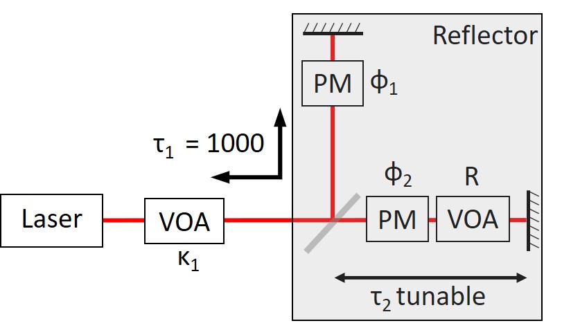
Figure 1: A representation of a semiconductor laser coupled to two mirrors at a distance. The Variable Optical Attenuators (VOAs) control the amount of light fed back to the laser cavity. $\tau_{1}$ and $\tau_{2}$ determine the delay or equivalently the distance where each mirror is positioned. The control of the feedback phases, $\phi_{1}$ and $\phi_{2}$, is visualized as Phase Modulators (PMs).

II Simulation Model and Methods

The simulated system is shown in figure 1 where a semiconductor laser is coupled to two mirrors at a distance. To study this system we use the following normalized Lang-Kobayashi equations, extended for double optical feedback [24, 17]:

$$\dot{E}(t)=\frac{1}{2}(1-i\alpha)N(t)E(t)+\kappa{}_{1}E(t-\tau_{1})\exp(\phi_{1})\\ +\kappa{}_{2}E(t-\tau_{2})\exp(\phi_{2}),$$ (1)

$$\dot{N}(t)=(P-N(t)-(1+2N(t))E^{2}(t)))/T,\\$$ (2)

with $E$ the electric field, and $N$ the carrier density in the laser cavity. The rate equations are fully normalized and the parameters are dimensionless. All time scales are normalized with respect to the photon lifetime. Details for the variables used can be found in table 1. For the laser parameters we use: $\alpha$ = 3, pump parameter $P=1$ (corresponding to 2 times the laser threshold), and carrier lifetime $T=1000$.

Each feedback arm has three parameters, the feedback rate ($\kappa_{i}$), the delay ($\tau_{i}$), and the feedback phase ($\phi_{i}$). We tune the feedback phase for either feedback loop separately from the delay. This allows us to investigate the impact on the laser dynamics of large changes in the delay versus sub-wavelength changes. In an experimental setup, this could be implemented as a translation stage, capable of large ($\sim{}mm$) steps, to change the large-scale delay, and small ($\sim{}10$ $nm$) steps to change the delay on the sub-wavelength level, essentially changing the feedback phase. For example, as in the setup in our earlier work [22].

Symbol	Represents	Typical value
$\alpha$	Linewidth enhancement factor	3
P	Pump parameter	1
T	Carrier lifetime	1000
$\kappa_{1}$	Feedback rate feedback loop 1	0–0.2
$\tau_{1}$	Delay feedback loop 1	1000
$\phi_{1}$	Feedback phase feedback loop 1	0–2$\pi$
$\kappa_{2}$	Feedback rate feedback loop 2	0–0.2
$\tau_{2}$	Delay feedback loop 2	647–1500
$\phi_{2}$	Feedback phase feedback loop 2	0–2$\pi$
$R=\kappa_{2}/\kappa_{1}$	Feedback rate ratio	/

Table 1: Details of the simulation parameters. In this paper we only change the feedback parameters ($\kappa_{1}$, $\tau_{1}$, $\phi_{1}$, $\kappa_{2}$, $\tau_{2}$, $\phi_{2}$). The laser parameters ($\alpha$, T, P) are fixed to these values.

The first feedback loop has a fixed delay of $\tau{}_{1}=1000$, while the delay of the second feedback loop ($\tau_{2}$) is varied. The second feedback rate ($\kappa_{2}$) and the feedback ratio R are not independent parameters: $R=\kappa_{2}/\kappa_{1}$. As we focus on the influence of the feedback parameters on the laser dynamics, we will change the first feedback rate ($\kappa_{1}$), feedback phase 1 ($\phi{}_{1}$), the feedback rate ratio ($R$), delay 2 ($\tau{}_{2}$), or the feedback phase 2 ($\phi{}_{2}$).

As a comparison, for a photon lifetime of 3 ps, a delay of $\tau_{1}=1000$ corresponds to a delay of $\tau^{\prime}=$3000\text{\,}\mathrm{ps}$$, which in terms to a mirror at a distance of approximately $l^{\prime}=\tau^{\prime}/2*c=$45\text{\,}\mathrm{cm}$$ in free space.

From the steady state solutions of the normalized equations without feedback ($\kappa_{1}=\kappa_{2}=0$ ) we can calculate the Relaxation Oscillation Frequency (ROF) $v_{RO}$ of the solitary laser. Following the same approach as described in ref. [1], the ROF is: $v_{RO}=\frac{1}{2\pi}\sqrt{\frac{2P}{T}-\frac{1}{4}(\frac{2P+1}{T})^{2}}$. Taking the inverse and filling in $P=1$ and $T=1000$, we find the Relaxation Oscillation Period (ROP): $\tau_{RO}=1/v_{RO}=141$.

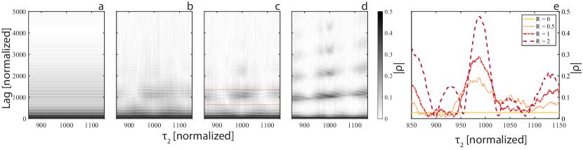
Figure 2: Evolution of the normalized autocorrelation of the intensity time-series when sweeping $\tau_{2}$. (a)–(d) for increasing values of $\kappa_{2}$: R = 0, 0.5, 1, 2. The white zones indicate almost no correlation. (e) Intersection of (a)–(d) at lag = 1000. In (c) Red lines indicate the lag window we use for the TDS optimization. Simulation parameters: $\tau_{1}=1000$, $\kappa_{1}=0.01$, $\phi_{1}=\phi_{2}=0$.

To study the dynamics we analyze the time series of the amplitude squared of the electric field: $|E|^{2}$, equivalent to the intensity. From this time series of intensity, we calculate the number of extrema. If there is only one extremum, the signal is constant and we consider the system to be in a steady state. If there are more extrema we consider the system is in a more complex state, from periodic to quasi-periodic and finally chaotic. In the case of 20 or more extrema we consider that the signal is chaotic, and this will be further motivated by the TDS and chaotic bandwidth analyses.

III Results and Discussion

Ideally, in the context of applications, the output of the laser should be chaotic with a non-detectable TDS while having the highest possible chaotic complexity. In the first subsection, we investigate how to optimize the TDS suppression and how the feedback phases come into play. In the second subsection, we discuss the complexity of the proposed optimized system by calculating the chaotic bandwidth. Finally, we study the stability of the system. We show that at high feedback rates, the system can go from stable to chaotic by a change of the feedback phase, implying that feedback phase control is especially crucial.

III.1 Time Delay Signature Suppression

We will optimize this system to suppress the TDS as much as possible using a second delay. This has already been shown in ref. [9]. The authors highlight that for case I, to suppress the TDS, the second delay should be close to the first delay. More specifically they mention that the suppression is strongest if $\Delta\tau=\tau_{2}-\tau_{1}\approx(-3/2)\tau_{\textrm{RO}},(-1/2)\tau_{\textrm{RO}},(1/2)\tau_{\textrm{RO}},(3/2)\tau_{\textrm{RO}}$, with $\tau_{\textrm{RO}}$ the ROP and for the case $R\approx 1$. They point out that the local minima in the autocorrelation occur with a period of $\tau_{\textrm{RO}}/2$, which is similar to the case of only one delay [25]. This strategy can be thought of as using the second delay to damp the oscillations due to the first delay. We start from these results to have a baseline before moving on to optimizing this system taking all feedback parameters into account.

To identify the TDS, manifesting itself due to a fixed time delay in the system, we apply the normalized autocorrelation function to the intensity time series. We calculate the autocorrelation ($\rho$) as defined in ref. [26]. As this function measures the linear correlation of the time series with a lagged version of itself, the TDS appears as a peak at the lag corresponding to the delay. Typically, we take the absolute value to focus on either the lack of correlation (i.e. values close to 0) or significant correlation (large positive values). Although there exist other functions to measure the TDS [8], for simplicity, we shall stick only to the autocorrelation.

In the first simulation, we vary the second delay and confirm the impact on the TDS (figure 2). For now, we keep the feedback rate fixed, $\kappa_{1}=0.01$, but do increase the second feedback rate and therefore increase $R$. For all of these simulations, the number of extrema is more than or equal to 20, indicating a highly complex state. In figure 2(a)–(d) we plot the absolute autocorrelation when varying $\tau_{2}$. By increasing the second feedback rate the TDS can be suppressed, although this depends strongly on the second delay value.

Our simulations confirm the earlier findings from Ref. [9]. In addition, even for different feedback ratios ($R$), the results remain qualitatively the same. Figure 2(e) shows the autocorrelation of (a)–(d) at lag = 1000. Here, we compare the different plots for a line along lag = 1000, which shows that only at specific $\tau_{2}$ the TDS is more suppressed. As we are increasing $R$ for these simulations but keeping $\kappa_{1}=0.01$, the total feedback rate is rising from figure 2 (a)–(d). The maximum height of the TDS depends on the total feedback rate, which was already shown in ref. [9] and this is similar to the one delay case [25].

However, focusing on only the autocorrelation value at lag = 1000 is limiting, as even a TDS close to the actual delay has to be suppressed. Therefore, we will use a lag window where we look for the TDS. In this window, our aim is to reduce the highest level of autocorrelation. To do so, we try to minimize the maxixum autocorrelation peak in this window. By keeping this peak small, the TDS is suppressed. Essentially, we track in a window: $\lvert\rho_{\textrm{max}}\rvert=max(\lvert autocorrelation(|E|^{2})\rvert)$. We take the total size of the window based on the ROP. As the period between minima is $\tau_{\textrm{RO}}/2$, we take the total size of the window equal to $5\tau_{\textrm{RO}}$ around lag = $\tau_{1}$. For our specific system, this comes down to a window of $W=\tau_{1}\pm 5\tau_{\textrm{RO}}/2\approx 1000\pm 353$ (shown with red lines in figure 2(c)).

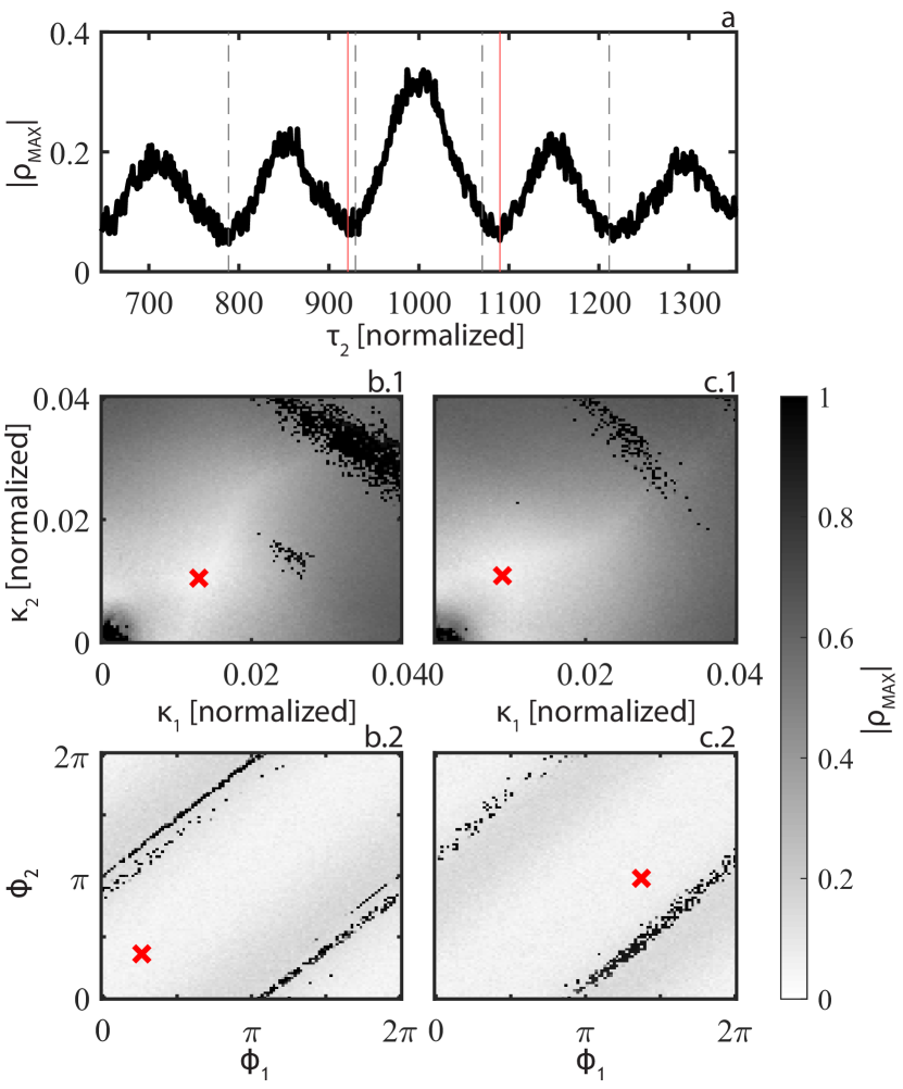
Figure 3: Optimization of the TDS suppression. (a) Sweeping $\tau_{2}$, (b.1) and (c.1) sweeping the feedback rates, (b.2) and (c.2) sweeping the feedback phases. (a) dotted black lines indicate: $\Delta\tau=\tau_{2}-\tau_{1}=-3\tau_{\textrm{RO}}/2,-\tau_{\textrm{RO}}/2,\tau_{\textrm{RO}}/2,3\tau_{\textrm{RO}}/2$. Full red lines indicate the minimum value closest to $\tau_{1}$. In (b) $\tau_{2}=921$, (c) $\tau_{2}=1090$, where for (b.1) and (c.1) $\phi_{1}=\phi_{2}=0$, and for (b.2) and (c.2) the feedback rates values used are indicated by the red crosses in (b.1) and (c.1). Red crosses are at the minimum of each map.

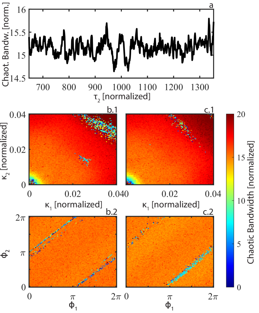
Figure 4: Chaotic bandwidth when optimizing the TDS suppression. (a) Varying $\tau_{2}$, (b.1) and (c.1) sweeping the feedback rates, (b.2) and (c.2) sweeping the feedback phases. The same simulation parameters as in figure 3 are used.

The results in figure 2 show that the TDS depends on the second delay and feedback rate. On the other hand, we showed that the feedback phases are important for the stability [23] and that it also impacts the TDS experimentally [22]. So to do a full TDS optimization we will now take into account all feedback parameters($\kappa_{1}$, $\tau_{1}$, $\phi_{1}$, $\kappa_{2}$, $\tau_{2}$, and $\phi_{2}$).

We start our optimization for $R=1$ (figure 2(c)) and apply it to minimize the TDS for $\tau_{2}$ both smaller and larger than $\tau_{1}$. To find a robustly suppressed TDS we propose the following optimization steps:

1. choose a second delay close to the first delay, around $\lvert\Delta\tau\rvert=\lvert\tau_{2}-\tau_{1}\rvert<5\tau_{\textrm{RO}}/2$, such that the TDS is maximally suppressed,

2. sweep $\kappa_{1}$ and $\kappa_{2}$ to find a robust suppression of the main TDS peak,

3. sweep $\phi_{1}$ and $\phi_{2}$ to find a robust suppression of the main TDS peak.

In the first step, shown in figure 3(a), we want to find a TDS minimum to start from. The dotted black lines indicate $\Delta\tau=\tau_{2}-\tau_{1}=-3\tau_{\textrm{RO}}/2,-\tau_{\textrm{RO}}/2,\tau_{\textrm{RO}}/2,3\tau_{\textrm{RO}}/2$, where we expect the optimal suppression based on Ref. [9]. This should be regarded as a rule of thumb as the lag at which the maximum TDS peak occurs shifts slightly depending on specific feedback parameters. Indeed, the red lines in figure 3(a), indicate that the local maximum suppression is at different values. We will optimize for a $\tau_{2}$ value below and above $\tau_{1}$. We take the local minima closest to $\tau_{1}$: $\tau_{2}=921$ and $\tau_{2}=1090$. For these points, the maximum autocorrelation value in the lag window becomes respectively $\lvert\rho_{\textrm{max}}\rvert=$6.12\text{\times}{10}^{-2}$$ and $\lvert\rho_{\textrm{max}}\rvert=$5.24\text{\times}{10}^{-2}$$. Although the (slightly) better suppression is actually for the second delay further away from the first, we assume that having the two delays closer makes it more difficult to detect them both.

We further optimize the TDS by sweeping both $\kappa_{1}$ and $\kappa_{2}$ and trying to find a more robust value for which a region around the main TDS peak is suppressed (shown in figure 3(b.1) and (c.1)). For the case of $\tau_{2}=921$, we find a minimal TDS at $\kappa_{1}=$1.29\text{\times}{10}^{-2}$$ and $\kappa_{2}=$1.04\text{\times}{10}^{-2}$$, with $\lvert\rho_{\textrm{max}}\rvert=$3.53\text{\times}{10}^{-2}$$. For $\tau_{2}=1090$, we find the minimal TDS at $\kappa_{1}=$8.89\text{\times}{10}^{-3}$$ and $\kappa_{2}=$1.08\text{\times}{10}^{-2}$$, with $\lvert\rho_{\textrm{max}}\rvert=$4.72\text{\times}{10}^{-2}$$.

For both cases overall the autocorrelation peak rises when increasing the feedback rates. In the black region in the top right of figure 3(b.1) and (c.1) the autocorrelation peak takes on high values. For these regions, the number of extrema can be below 20, indicating that the system is not chaotic anymore. In addition, we note that the position of the strongest TDS peaks in the lag window latches on to the lag = $\tau_{i}$ of the strongest feedback loop, around $R=1$ is the transition.

In our final step, we further optimize the TDS by sweeping the feedback phases, shown in figure 3(b.2) and (c.2). For the case of $\tau_{2}=921$ the minimum is reached for $\phi_{1}=0.825$ and $\phi_{2}=1.13$, for which $\lvert\rho_{\textrm{max}}\rvert=$2.76\text{\times}{10}^{-2}$$. For the case of $\tau_{2}=1090$ the minimum is reached for $\phi_{1}=4.32$ and $\phi_{2}=3.08$, for which $\lvert\rho_{\textrm{max}}\rvert=$2.54\text{\times}{10}^{-2}$$. So by optimizing the feedback phases we further suppress the TDS almost twofold.

As indicated by the black regions, the maximum autocorrelation peak can take on high values by just sweeping the feedback phases. This shows that for optimal suppression, one needs to take into account the feedback phases and can not only optimize the large scale delay values, confirming our experimental results in Ref. [22]. As similar autocorrelation values mostly lie on diagonals, the main parameter that should be taken into account is the feedback phase difference. Of course, this effect works both ways: if, for some reason, an additional feedback phase term is added to the system, suppressing the TDS by choosing the second delay might only have a limited effect.

III.2 Chaos Bandwidth Optimization

Figure 5: Evolution of the chaotic bandwidth versus the feedback parameters. (a) Sweep of the feedback phases, around the optimum point of TDS in figure 3 (c.2), (a.1) sweeping $\phi_{1}$, (a.2) sweeping $\phi_{2}$. (b) Sweep of the feedback rates. Black full line: sweeping feedback rates along optimal from 3 (c.2), $R=1.2$, $\tau_{2}=1090$, $\phi_{1}=4.32,\phi_{2}=3.08$. The dotted red line is the case for only one delay ($R=0$, $\tau_{1}=1000$, $\phi_{1}=0$).

Besides suppressing the TDS we want to optimize the complexity of the system. Beyond a certain number of extrema in the intensity time series, there is no longer useful information to discriminate the nature of the dynamics. Therefore, we look at another figure of merit to see the impact of the second delay on the laser dynamics: the chaotic bandwidth (CBW). We will use this metric to study how the feedback parameters affect the complexity of the system. It gives a rough but useful estimation of the complexity and unpredictability of the laser behavior [19]. To calculate it we take the RF spectrum from the time series and only consider the bandwidth contributing to 80 % of the power, as described in ref. [19]. Although our simulations are normalized, the CBW units would correspond to GHz when we assume a photon lifetime of 1 ps (although 3 to 5 ps might be more realistic).

We study the same parameter regions as before but now focus on the CBW. The results are shown in figure 4. Changing $\tau_{2}$ does not have a clear impact (see figure 4(a)) in this range, except for two minima around $\tau_{2}=1000$. Overall the total variation is below 10 %. When changing the feedback rate there is a clear impact on the CBW, shown in figure 4(b.1) and (c.1). Overall the CBW rises when increasing either $\kappa_{1}$ or $\kappa_{2}$. The more optical feedback there is the higher the CBW. However, at high feedback rates, the same stability regions show themselves here. We shall discuss them further in the next subsection. When changing either feedback phase, shown in figure 4(b.2) and (c.2) there is a small impact on the CBW, although the quantitative change is small, on the order of 10 %.

Figure 5(a.1) and (a.2) show a line along the maps shown earlier for the CBW to have a closer look. Here we only sweep one feedback phase while keeping the other one fixed at zero. In this way, we see that there is a small impact due to the feedback phase. However, the total impact is rather limited, in the order of 5 %. The regions where the CBW jumps are again regions where the system restabilizes. For the optimal TDS suppression case, the CBW is $15.31$ for $\tau_{2}=921$ and $15.19$ for $\tau_{2}=1090$. Changing the feedback parameters slightly around this optimum value has almost no impact on the CBW.

However, when optimizing for the CBW we see that it does increase significantly when either $\kappa_{1}$ or $\kappa_{2}$ is increased, as long as the system is not in a steady state. Figure 5(b) shows the case for $R=0$ (dotted red line) and $R=1$ (full black line). When increasing the feedback rates the CBW overall rises. The CBW in this range for the case of two delays is always higher than the case of only one delay, although they are very close around $\kappa_{1}=0.01$. For the two delay case, the CBW rises faster with respect to the feedback rate. However, because $R=1.2$, the energy returning to the laser rises faster, which could explain the discrepancy. Before $\kappa_{1}=0.003$, around $\kappa_{1}=0.025$, $\kappa_{1}=0.035$, and $\kappa_{1}=0.045$ the system can have less than 20 extrema and the CBW takes on nonsense values. When discarding these regions the relation between the feedback rate and CBW is almost linear. We then apply a linear regression for each case from $\kappa_{1}=0.02$ to $0.05$. The slope of the one delay case is $1.39\text{\times}{10}^{-2}$ while the slope of the two delay case is $2.62\text{\times}{10}^{-2}$. The ratio between both is $1.88$, so the two delay case rises faster but not twice as fast. The case for $\tau_{2}=921$ is qualitatively the same.

In summary, our simulations show that the CBW mostly changes when changing the feedback rate, but is rather robust when either $\tau_{2}$ or the feedback phases are changing, as long as the system is still chaotic. However, even when changing the feedback rate the relative change in CBW is rather limited over the range where the TDS is most suppressed. On the other hand, when you want to optimize the CBW increasing the feedback rate is the way to go, if the system can remain chaotic.

III.3 Restabilization at high feedback rates

We want to keep the system in a chaotic state, therefore we have to avoid stable regions. As shown above, for strong feedback rates the system can restabilize. Moreover, with a small change of the feedback phases the system can switch between chaotic and stable. In the previous section, we saw that the CBW increases with increased feedback rate. If one wants to optimize the CBW without interest in the TDS, increasing the feedback rate is an option. However, it then becomes essential to avoid the regions of stability. In this part, we investigate these regions of higher feedback rates to show when and why the restabilization occurs.

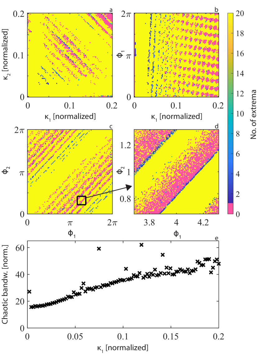
Figure 6: Restabilization at high feedback rates. Pink indicates a steady state, and yellow indicates a complex state. (a) Number of extrema when sweeping the feedback rates ($\kappa_{1}$ and $\kappa_{2}$). Simulation parameters: $\tau_{1}=1000$, $\tau_{2}=1090$, $\phi_{1}=\phi_{2}=0$. (b) Sweep along the diagonal ($R=1$) of (a) and sweeping $\phi_{1}$ while keeping $\phi_{2}=0$. (c) Number of extrema when sweeping both feedback phases ($\phi_{1}$ and $\phi_{2}$). Simulation parameters: $\tau_{1}=1000$, $\tau_{2}=1090$, $\kappa_{1}=\kappa_{2}=0.1$. (d) Zoom in on the square in map (c). (e) The same parameters as in (b) are used but $\phi_{1}$ is chosen such that the chaotic bandwidth is optimized.

First, we investigate the impact of the feedback rates on the stability. We start from a good position to suppress the TDS: $\tau_{2}=1090$. With the feedback phases set to zero, we then sweep the feedback rates to get the map shown in figure 6(a). Pink indicates a steady state (1 extremum) while yellow indicates a complex state ($\geq$ 20 extrema). For high feedback rates, the laser behavior can become less complex and even reach a steady state again. For these restabilizations to occur both $\kappa_{1}$ and $\kappa_{2}$ need to pass a certain threshold. After this threshold, when further increasing $\kappa_{1}$ and $\kappa_{2}$, the system will every so often settle down to a steady state again.

These regions of restabilization are feedback phase dependent as shown in figure 6(b)–(d). Furthermore, above a certain feedback rate threshold, the laser system can always restabilize by setting the feedback phases. For each point along the $R=1$ line in figure 6(a), we sweep $\phi_{1}$ while $\phi_{2}=0$. The results are shown in figure 6(b). By tuning the feedback phase difference the system can always become stable for $\kappa_{1}\geq 0.059$. However, for an even lower threshold $\kappa_{1}\geq 0.026$ the system settles down to a periodic state for specific feedback phase values. Above the first Hopf bifurcation and below this last threshold the system remains complex when sweeping the feedback phases, so to be used as a robust chaotic system you should remain in this region unless precise control of the mirror position is possible.

Now, we fix the feedback rates ($\kappa_{1}=\kappa_{2}=0.1$) and sweep both feedback phases. The results are shown in figure 6(c). By doing so, the laser switches between stable and chaotic. From our simulations, it seems to be a general feature that these restabilization regions, which are surrounded by chaotic regions in the feedback rates parameter space, are feedback phase dependent. We verified that similar behavior occurred in the presence of spontaneous emission noise.

By zooming in on a part of the map, shown in figure 6 (d), we see that there is a broad region of steady states. However, here and there the system can still become chaotic. The lower right part of this stability region has a small region where the laser behavior is periodic.

If the feedback phase can be controlled it is possible to reach very high CBW values. In figure 6 (e) we show a sweep of $\kappa_{1}$ while choosing $\phi_{1}$ such that 1) the number of extrema is $\geq 20$ and 2) that the CBW is maximized (other parameters: $R=1$, $\phi_{2}=0$). For feedback rate values up to $0.1$, we see an extension of the linear region discussed in the previous section. However, by setting the feedback phase we now avoid the restabilization regions. For higher feedback rates the CBW increases at a slower rate. As we confirm that the number of extrema is 20 or more for this simulation, the outliers around CBW = 60 are not stable. Understanding what is happening different there is outside the scope of this paper.

We hypothesize that these restabilizations occur due to constructive interference occurring in the feedback section. We support this by looking at the effective phase difference between both feedback sections when taking into account the shift in the laser wavelength as well as the delays and feedback phases, similarly defined in ref. [23]:

$$\Delta\phi_{\textrm{eff}}=(\tau_{2}-\tau_{1})\delta+\phi_{2}-\phi_{1},$$ (3)

in which we estimate the wavelength ($\delta$) by taking the average of $\delta=\frac{d\phi(t)}{dt}$. When looking at this effective phase difference (figure 7) the stable regions occur when both feedback loops are in phase, essentially when they are a multiple of $2\pi$. Although this should be confirmed with a more in-depth investigation, it is possible that when both feedback loops are in phase, the system is close to the equivalent system of a laser with one strong feedback loop. If so, this case would be close to the case of the region V in the diagram of feedback regimes in a semiconductor laser [27, 3]. Of course, this is with the exception that this region now can become chaotic when changing the feedback phases.

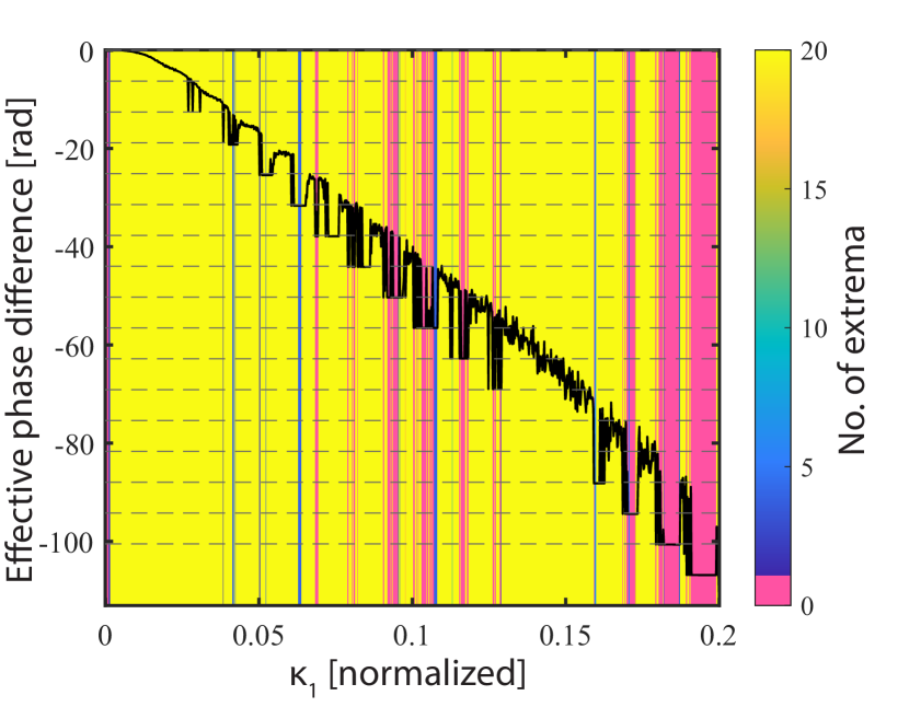
Figure 7: Evolution of the effective phase in the feedback section versus the stability of the system. Dotted straight lines indicate effective phase is in phase (multiple of $2\pi$). Simulation parameters: $\tau_{2}=1090$, $\kappa_{2}=\kappa_{1}$, $\phi_{1}=\phi_{2}=0$.

In summary, to remain chaotic without sensitivity to feedback phase changes, you should remain at intermediate feedback rate values. Of course, if it’s possible to control the feedback phases higher, CBW can be reached by avoiding the stability regions. We attribute this sensitivity to the feedback phases due to interference occurring in the feedback section. Although we only showed the simulations for one specific second delay value, this behavior occurs for a wide second delay range around the first delay.

IV Conclusion

We numerically studied a semiconductor laser coupled to two mirrors at a distance. Our goal was to optimize this system to suppress the TDS and have a high CBW. We showed how to optimize the TDS suppression when taking into account all the feedback parameters. Building upon the work of ref. [9] we confirm that when the delays are close to each other the TDS can be suppressed. However, we confirm here numerically that the feedback phases have to be controlled to effectively suppress the TDS, as we already showed for a particular case experimentally [22]. Moreover, we show that control of the feedback phases is actually essential to suppress the TDS, of which a small shift can lead to a much higher TDS peak. By taking into account all the feedback parameters it is possible to strongly suppress the TDS.

We studied the complexity of this optimized system by calculating the CBW. We show that the TDS can be suppressed without loss of CBW. Changing the feedback parameters around the maximally suppressed TDS almost has no change on the CBW. Our results show that the CBW increases significantly when increasing the feedback rates, as long as the feedback phase is controlled.

In this context, we investigated the system for higher feedback rates. We show that above a certain threshold of the feedback rates, it is always possible to switch from a chaotic to a steady state by changing the feedback phase. We use this to push the CBW much higher when controlling the feedback phase. We attribute this behavior to constructive interference occurring in the feedback section.

In conclusion, when taking into account all feedback parameters it is possible to use this system to get a chaotic laser with high CBW and strongly suppressed TDS, due to the additional mirror. Or, if TDS suppression is not crucial, the system can be optimized for high CBW only. However, control of all feedback parameters is crucial. A system implemented on Photonic Integrated Circuits (PICs) could reach the needed precision to have an optimized chaotic laser.

One parameter that should be investigated further in this context is the ROF of the laser. This parameter has an impact on the ease of TDS detection in the one delay case [25] and comes into play in the dual delay system when setting the second delay. So, further investigation in this context could further optimize this chaotic laser system.

References

References

- [1] J. Ohtsubo, Semiconductor Lasers, vol. 111 of Springer Series in Optical Sciences. Berlin, Heidelberg: Springer Berlin Heidelberg, 2013.
- [2] A. Uchida, Optical Communication with Chaotic Lasers. Weinheim, Germany: Wiley-VCH Verlag GmbH and Co. KGaA, 2012.
- [3] S. Donati and R. H. Horng, “The diagram of feedback regimes revisited,” IEEE Journal on Selected Topics in Quantum Electronics, vol. 19, no. 4, 2013.
- [4] I. Reidler, Y. Aviad, M. Rosenbluh, and I. Kanter, “Ultrahigh-Speed Random Number Generation Based on a Chaotic Semiconductor Laser,” Physical Review Letters, vol. 103, no. 2, p. 024102, 2009.
- [5] V. S. Udaltsov, L. Larger, J. P. Goedgebuer, A. Locquet, and D. S. Citrin, “Time delay identification in chaotic cryptosystems ruled by delay-differential equations,” Journal of Optical Technology, vol. 72, no. 5, p. 373, 2005.
- [6] V. Z. Tronciu, I. V. Ermakov, P. Colet, and C. R. Mirasso, “Chaotic dynamics of a semiconductor laser with double cavity feedback: Applications to phase shift keying modulation,” Optics Communications, vol. 281, no. 18, pp. 4747–4752, 2008.
- [7] Y. K. Chembo, D. Brunner, M. Jacquot, and L. Larger, “Optoelectronic oscillators with time-delayed feedback,” Reviews of Modern Physics, vol. 91, no. 3, p. 35006, 2019.
- [8] X. Wei, L. Qiao, M. Chai, and M. Zhang, “Review on the broadband time-delay-signature-suppressed chaotic laser,” Microwave and Optical Technology Letters, vol. 64, no. 12, pp. 2264–2277, 2022.
- [9] J.-G. Wu, G.-Q. Xia, and Z.-M. Wu, “Suppression of time delay signatures of chaotic output in a semiconductor laser with double optical feedback,” Optics Express, vol. 17, no. 22, p. 20124, 2009.
- [10] M. W. Lee, P. Rees, K. A. Shore, S. Ortin, L. Pesquera, and A. Valle, “Dynamical characterisation of laser diode subject to double optical feedback for chaotic optical communications,” IEE Proceedings: Optoelectronics, vol. 152, no. 2, pp. 97–102, 2005.
- [11] S. K. Tavakoli and A. Longtin, “Multi-delay complexity collapse,” Physical Review Research, vol. 2, no. 3, p. 033485, 2020.
- [12] A. Többens and U. Parlitz, “Dynamics of semiconductor lasers with external multicavities,” Physical Review E - Statistical, Nonlinear, and Soft Matter Physics, vol. 78, no. 1, 2008.
- [13] Yun Liu and J. Ohtsubo, “Dynamics and chaos stabilization of semiconductor lasers with optical feedback from an interferometer,” IEEE Journal of Quantum Electronics, vol. 33, no. 7, pp. 1163–1169, 1997.
- [14] F. R. Ruiz-Oliveras and A. N. Pisarchik, “Phase-locking phenomenon in a semiconductor laser with external cavities,” Optics Express, vol. 14, no. 26, p. 12859, 2006.
- [15] D. W. Sukow, M. C. Hegg, J. L. Wright, and A. Gavrielides, “Mixed external cavity mode dynamics in a semiconductor laser,” Optics Letters, vol. 27, no. 10, p. 827, 2002.
- [16] C. Onea, P. E. Sterian, I. R. Andrei, and M. L. Pascu, “High frequency chaotic dynamics in a semiconductor laser with double-reflector selective cavity,” UPB Scientific Bulletin, Series A: Applied Mathematics and Physics, vol. 81, no. 4, pp. 261–270, 2019.
- [17] F. Rogister, P. Mégret, O. Deparis, M. Blondel, and T. Erneux, “Suppression of low-frequency fluctuations and stabilization of a semiconductor laser subjected to optical feedback from a double cavity: theoretical results,” Optics Letters, vol. 24, no. 17, p. 1218, 1999.
- [18] W. A. S. Barbosa, E. J. Rosero, J. R. Tredicce, and J. R. Rios Leite, “Statistics of chaos in a bursting laser,” Physical Review A, vol. 99, no. 5, p. 053828, 2019.
- [19] F.-Y. Lin, Y.-K. Chao, and T.-C. Wu, “Effective Bandwidths of Broadband Chaotic Signals,” IEEE Journal of Quantum Electronics, vol. 48, no. 8, pp. 1010–1014, 2012.
- [20] V. Z. Tronciu, C. R. Mirasso, and P. Colet, “Chaos-based communications using semiconductor lasers subject to feedback from an integrated double cavity,” Journal of Physics B: Atomic, Molecular and Optical Physics, vol. 41, no. 15, p. 155401, 2008.
- [21] M. W. Lee, L. Larger, V. Udaltsov, É. Genin, and J.-P. Goedgebuer, “Demonstration of a chaos generator with two time delays,” Optics Letters, vol. 29, no. 4, p. 325, 2004.
- [22] R. de Mey, S. W. Jolly, A. Locquet, and M. Virte, “Chaotic time-delay signature suppression in lasers using phase-controlled dual optical feedback,” Optics Continuum, vol. 1, no. 10, p. 2127, 2022.
- [23] R. de Mey, S. W. Jolly, and M. Virte, “Clarifying the impact of dual optical feedback on semiconductor lasers through analysis of the effective feedback phase,” arXiv, no. 2306.04006, 2023.
- [24] R. Lang and K. Kobayashi, “External optical feedback effects on semiconductor injection laser properties,” IEEE Journal of Quantum Electronics, vol. 16, no. 3, pp. 347–355, 1980.
- [25] D. Rontani, A. Locquet, M. Sciamanna, and D. S. Citrin, “Loss of time-delay signature in the chaotic output of a semiconductor laser with optical feedback,” Optics Letters, vol. 32, no. 20, p. 2960, 2007.
- [26] Y. Wu, Y. C. Wang, P. Li, A. B. Wang, and M. J. Zhang, “Can fixed time delay signature be concealed in chaotic semiconductor laser with optical feedback?,” IEEE Journal of Quantum Electronics, vol. 48, no. 11, pp. 1371–1379, 2012.
- [27] R. W. Tkach and A. R. Chraplyvy, “Regimes of feedback effects in 1.5-um distributed feedback lasers,” Journal of Lightwave Technology, vol. LT-4, no. 11, pp. 1655–1661, 1986.