Fourier Calculus from Intersection Theory

Abstract

Building on recent advances in studying the co-homological properties of Feynman integrals, we apply intersection theory to the computation of Fourier integrals. We discuss applications pertinent to gravitational bremsstrahlung and deep inelastic scattering in the saturation regime. After identifying the bases of master integrals, the latter are evaluated by means of the differential equation method. Finally, new results with exact dependence on the spacetime dimension $\mathrm{D}$ are presented.

I Introduction

In recent years, monumental efforts have been invested in developing tools for evaluating Feynman integrals in particle physics. Modern state-of-the-art computations face the challenge of applying integration-by-parts (IBP) decompositions [1, 2] in the most efficient way possible. IBP identities are relations among Feynman integrals sharing a common set of denominators, appearing with different propagator powers (irreducible scalar products in the numerator can be dealt with as denominators with negative powers). These allow for the decomposition of any Feynman integral in terms of a finite spanning set of simpler and linearly independent integrals, often referred to as master integrals. The decomposition to master integrals is fundamentally a matter of linear algebra, and several publicly available computer programs can efficiently execute it [3, 4, 5, 6, 7, 8, 9, 10, 8, 11].

When recognized as twisted periods, Feynman integrals can alternatively be decomposed into master bases by making use of concepts and computing tools of de Rham twisted cohomology theory [12, 13, 14, 15], as first proposed in  [16, 17, 18, 19].

Within this framework, integrals are considered as pairings of regulated integration domains and differential $n$-forms, known as twisted cycles and cocycles respectively, which are elements of isomorphic vector spaces, equipped with inner products, called the intersection numbers. The intersection number can be used to derive the decomposition of Feynman integrals in terms of master integrals by projections, as an alternative to the system-solving procedure underpinning IBP decompositions.

Although the most recent applications of intersection theory have dealt with Feynman integrals [17, 18, 20, 19, 21, 22, 23, 24, 25, 26, 27, 28, 29, 30, 31], the method is rather general, and the range of its applications can be extended to a much wider class of cases, relevant for physical and mathematical studies (see, e.g., [32, 33, 34, 35]).

In this letter, we propose an intersection-theory based approach to the evaluation of dimensionally regularized Fourier transforms, herein referred to as Fourier integrals.

Indeed, as is the case for any Feynman integral, expressing any Fourier integral in Baikov representation [36] enables its identification as a twisted period. Thus, relations between Fourier integrals and, in particular, their decompositions into a common master integral basis, can be obtained directly from intersection numbers. Moreover, intersection theory can be used to derive the system of differential equations satisfied by the master Fourier integrals, which can be solved analytically (when possible) similarly to Feynman integrals. [37, 38, 39, 40].

To illustrate our method, we identify three cases of physical interest, requiring the evaluation of certain types of dimensionally regulated Fourier integrals: III.1 the scalar (Feynman) propagator in position space, III.2 the tree-level gravitational spectral waveform, and III.3 color dipole scattering in high-energy QCD. In each of the considered cases, intersection numbers are used to build linear relations and differential equations for the associated master integrals in Baikov representation. Once the systems of differential equations are obtained, the solutions are systematically derived, provided an appropriate set of boundary conditions. Using this approach, we present new, closed-form formulae for $\mathrm{D}$-dimensional Fourier integrals relevant to cases III.2 and III.3.

From a mathematical point of view, our results offer a generalization of the studies carried out on confluent hypergeometric integrals [14, 15], involving intersection numbers between $1$-forms, to cases where the evaluation of intersection numbers for $n$-forms is required.

This letter is organized as follows. In sec. II we provide the necessary background on intersection theory and outline its application to Fourier integrals. The method is then applied in sec. III, using the three cases of study (III.1, III.2 and III.3) mentioned above. For III.2 and III.3, a minimal physics background is provided for the reader’s convenience. In sec. IV, we present our conclusions and an outlook. The four appendices contain the derivation of the Baikov representation for Fourier integrals, and auxiliary formulae recalled in the text.

II Fourier integrals and intersection theory

In this section, we provide some background material on intersection theory and describe how it can be applied to dimensionally regularized Fourier integrals [16, 17, 18, 19] .

Twisted cohomology

We consider instances of twisted period integrals, which generically take the form

$$I=\int_{C_{R}}u(\mathbf{z})\varphi_{L}(\mathbf{z})\,,$$ (1)

where the twist $u(\mathbf{z})$ is a multivalued function, $\varphi_{L}(\mathbf{z})$ is an algebraic differential $n$-form and $C_{R}$ is a contour of integration. The latter is defined such that $u(\mathbf{z})$ vanishes on its boundary: $u(\mathbf{z})=0$ for any $\mathbf{z}\in\partial C_{R}$. This condition on $u$ together with eq. (1) give an equivalence relation between differential forms

$$\varphi_{L}\sim\varphi_{L}+\nabla_{\omega}\xi\,,$$ (2)

where $\xi$ is a differential $(n{-}1)$-form and

$$\nabla_{\omega}=\mathrm{d}+\omega\wedge\quad\text{with}\quad\omega=\mathrm{d}\log{u}\,.$$ (3)

The collection of all the equivalence classes forms the twisted cohomology group $H_{\omega}^{n}$. This group is always finite-dimensional and forms a vector space [17]. We denote an element by

$$\bra{\varphi_{L}}\in H_{\omega}^{n}\,.$$ (4)

As for any other finite dimensional vector space, there exists a dual vector space $H_{-\omega}^{n}$, denoted by

$$H_{-\omega}^{n}\ni\ket{\varphi_{R}}\,.$$ (5)

Using these definitions, we write the (dual) integrals in eq. (1) as a pairing between a (dual) cycle and a (dual) cocycle

$$I =\int_{C_{R}}u(\mathbf{z})\varphi_{L}(\mathbf{z})=\bra{\varphi_{L}}C_{R}]\,,$$ (6a)

$$=\int_{C_{L}}u(\mathbf{z})^{-1}\varphi_{R}(\mathbf{z})=[C_{L}\ket{\varphi_{R}}\,.$$ (6b)

Basis of master integrals

We can formally define bases for $H_{\omega}^{n}$ and its dual $H_{-\omega}^{n}$ as

$$\text{span}\{\bra{e_{1}},\ldots,\bra{e_{\nu}}\} =H_{\omega}^{n}\,,$$ (7a)

$$\text{span}\{\ket{\widecheck{e}_{1}},\ldots,\ket{\widecheck{e}_{\nu}}\} =H_{-\omega}^{n}\,,$$ (7b)

respectively. Both $H_{\omega}^{n}$ and $H_{-\omega}^{n}$ have the same dimension [41, 18], which can be computed as

$$\nu=\left\{\#\leavevmode\nobreak\ \text{of solutions to $\omega=0$}\right\}\,.$$ (8)

Any elements $\bra{\varphi_{L}}\in H_{\omega}^{n}$ and $\ket{\varphi_{R}}\in H_{-\omega}^{n}$ can then be decomposed with respect to the choice of (dual) bases

$$\bra{\varphi_{L}}=\sum_{i=1}^{\nu}c_{i}\bra{e_{i}}\quad\text{and}\quad\ket{\varphi_{R}}=\sum_{i=1}^{\nu}\widecheck{c}_{i}\ket{\widecheck{e}_{i}}\,.$$ (9)

By pairing the linear combinations in eq. (9) with the appropriate contours, we obtain the decompositions of the corresponding twisted periods with respect to the basis of master integrals $J_{i}=\bra{e_{i}}C_{R}]$ and $\widecheck{J}_{i}=[C_{L}\ket{\widecheck{e}_{i}}$

$$I =\bra{\varphi_{L}}C_{R}]=\sum_{i=1}^{\nu}c_{i}\bra{e_{i}}C_{R}]=\sum_{i=1}^{\nu}c_{i}J_{i}\,,$$ (10a)

$$=[C_{L}\ket{\varphi_{R}}=\sum_{i=1}^{\nu}\widecheck{c}_{i}[C_{L}\ket{\widecheck{e}_{i}}=\sum_{i=1}^{\nu}\widecheck{c}_{i}\widecheck{J}_{i}\,.$$ (10b)

Integral decompositions

Following [13, 16], we can introduce a scalar product $\braket{\bullet,\bullet}$ between elements of $H_{\omega}^{n}$ and $H_{-\omega}^{n}$, called the intersection number. With this additional structure, the coefficients $c_{i}$ can be extracted using the master decomposition formula [16, 17]

$$c_{i}=\sum_{j=1}^{\nu}\braket{\varphi_{L},\widecheck{e}_{j}}(C^{-1})_{ji}\quad\text{with}\quad C_{ij}=\braket{e_{i},\widecheck{e}_{j}}\,.$$ (11)

The computation of intersection numbers in eq. (11) has been the primary focus of recent work in intersection theory, with significant progress made over the past few years [42, 19, 43, 44, 45, 29].

In the univariate case ($n=1$), a compact formula for the intersection number is known and given by

$$\braket{\varphi_{L},\varphi_{R}}=\sum_{p\in\mathcal{P}}\text{Res}_{z=p}\left(\psi\varphi_{R}\right)\,,$$ (12)

where $\mathcal{P}$ is the set of $\omega$’s poles, and $\psi$ satisfies the differential equation

$$\nabla_{\omega}\psi=\varphi_{L}\,.$$ (13)

The calculation of multivariate intersection numbers requires more effort and there are several strategies [13, 46, 18, 20, 25, 47, 45, 27, 29]. In this letter, we adopt the ones introduced in [29, 25, 26, 18, 31].

As mentioned earlier, the computation of intersection numbers allows us to build the differential equation $\bm{\Omega}_{x}$ satisfied by the basis of master integrals in any external variable $x$

$$\partial_{x}J_{i}=[\bm{\Omega}_{x}]_{ij}J_{j}\,.$$ (14)

To see this, we note that in the language of twisted cohomology, eq. (14) translates to

$$\partial_{x}\bra{e_{i}} =\bra{\partial_{x}(ue_{i})/u}=[\bm{\Omega}_{x}]_{ij}\bra{e_{j}}\,,$$ (15)

which implies

$$[\bm{\Omega}_{x}]_{ij} =\braket{\partial_{x}(ue_{i})/u,\widecheck{e}_{k}}[C^{-1}]_{kj}\,.$$ (16)

We reiterate that the derivations of eqs. 11 and 16 do not involve solving (potentially large) systems of linear equations but instead exclusively rely on the computation of intersection numbers.

Fourier integrals in Baikov representation

We consider a generic $\mathrm{D}$-dimensional Fourier integral, which takes the form

$$\tilde{f}(\{x_{i}\})=\int f(\{q_{i}\})\prod_{j=1}^{L}\mathrm{e}^{iq_{j}\cdot x_{j}}{\text{d}\bar{}\hskip 1.00006pt}^{\mathrm{D}}q_{j}\,,$$ (17a)

$$\text{with measure:}\qquad{\text{d}\bar{}\hskip 1.00006pt}^{\mathrm{D}}q_{j}=\frac{\mathrm{d}^{\mathrm{D}}q_{j}}{(2\pi)^{\mathrm{D}/2}}\,.$$ (17b)

Eq. (17) is the Fourier transform of the function/distribution $f$ performed over $L$ internal vectors $\{q_{i}\}$. The result is a function of $E$ external vectors $\{x_{i}\}$. We denote the set of $n=\frac{L}{2}(L{+}1){+}LE$ internal scalar products as

$$S_{i}=\{q_{1}^{2},q_{1}\cdot q_{2},\dots,q_{L}^{2},q_{1}\cdot x_{1},q_{1}\cdot x_{2},\dots,q_{L}\cdot x_{E}\}\,.$$ (18)

To reinterpret the Fourier transform in eq. (17) as a twisted period, we propose to change variables to the Baikov variables [36, 48]: the procedure involves a first change of variables from the internal vectors $q_{i}$ to the internal scalar products $S_{i}$, followed by a second change of variables,

$$z_{i}=A_{ij}\,S_{j}+B_{j}\,,$$ (19)

where $A_{ij}$ is an $n\times n$ matrix and $B_{j}$ is an $n$-dimensional vector. Both operations only depend on the external scalar products $\{S_{i}\}$. Once the dust settles, the result reads

$$\tilde{f}=\int_{C_{R}}u(\mathbf{z})\,\varphi_{L}(\mathbf{z})\,,$$ (20)

where

$$C_{R}=\bigcap_{i=1}^{L}\left\{\frac{\det G_{\{q_{i},\ldots,q_{L},y_{1},\ldots,y_{E}\}}}{\det G_{\{q_{i+1},\ldots,q_{L},y_{1},\ldots,y_{E}\}}}>0\right\}\,,$$ (21)

is the contour of integration. The differential form $\varphi_{L}(\mathbf{z})=f(\mathbf{z})\,\mathrm{d}^{n}\mathbf{z}$ contains the function/distribution $f$ we would like to Fourier transform and

$$u(\mathbf{z})=\kappa\ \mathrm{e}^{ig(\mathbf{z})}B(\mathbf{z})^{\frac{\mathrm{D}-L-E-1}{2}}\,,$$ (22)

is the twist. Here, $g(\mathbf{z})$ is always linear in $\mathbf{z}$ and we define

$$G(\{x\}) =\det[x_{i}\cdot x_{j}]\,,$$ (23a)

$$B(\mathbf{z}) =G(q_{1},\dots,q_{L},y_{1},\dots,y_{E})\,,$$ (23b)

$$\kappa =\frac{\pi^{\frac{L(1-L-2E)}{4}}G(y_{1},\dots,y_{E})^{\frac{E-\mathrm{D}+1}{2}}}{2^{\frac{L\mathrm{D}}{2}}\det A\prod_{j=1}^{L}\Gamma\left(\frac{\mathrm{D}{-}L{-}E+j}{2}\right)}\,.$$ (23c)

Note that $B\geq 0$ on $C_{R}$. Complementary details regarding the derivation of eq. (20) can be found in app. A.

Representing a Fourier integral as the twisted period in eq. (20) enables the use of intersection theory for the construction of differential equation (c.f., eq. (14)). Thus, the master Fourier integrals $J_{i}$ can be evaluated by solving the system of differential equations, analogously to Feynman integrals.

III Applications

In this section, we apply the formalism described above to three families of Fourier integrals arising in various corners of particle physics. An ancillary Mathematica file (ancillary.m) containing complementary details for each example is attached to the preprint version of this letter.

Below, $\mathcal{M}=\mathbbm{R}^{1,\mathrm{D}-1}$ denotes the Minkowski spacetime manifold. Unless specified otherwise, we work in the mostly plus Lorentzian signature $(-,+,+,...,+)$.

III.1 Fourier transform of a scalar propagator

As a first example, we consider the Fourier transform of a massive scalar Feynman propagator,

$$I_{n}=\int_{\mathcal{M}}{\text{d}\bar{}\hskip 1.00006pt}^{\mathrm{D}}q\frac{\mathrm{e}^{iq\cdot x}}{(q^{2}+m^{2}-i\varepsilon)^{n}}\,.$$ (24)

We work with dimensionless integrals $K_{n}$, defined by

$$I_{n}=m^{\mathrm{D}{-}2n}K_{n}\,,\leavevmode\nobreak\ \leavevmode\nobreak\ K_{n}=\int_{\mathcal{M}}{\text{d}\bar{}\hskip 1.00006pt}^{\mathrm{D}}k\frac{\mathrm{e}^{ik\cdot v}}{(k^{2}{+}1{-}i\varepsilon)^{n}}\,,$$ (25)

where $v=mx$ and $k=q/m$ are both dimensionless vectors. For $K_{n}$, we have $L=1$ internal vector $\{k\}$ and $E=1$ external vector $\{v\}$. We define the $n=2$ integration variables as $z_{1}=k^{2}+1$ and $z_{2}=k\cdot v$. Thus, in the Baikov representation, this integral takes the form

$$K_{n}=\int\frac{\mathrm{d}\mathbf{z}}{z_{1}^{n}}u(\mathbf{z})\ ,$$ (26)

where the twist is given by

$$u(z_{1},z_{2})=\frac{\mathrm{e}^{iz_{2}}\tau^{\frac{2-\mathrm{D}}{2}}}{2^{\frac{\mathrm{D}}{2}}\sqrt{\pi}\Gamma((\mathrm{D}-1)/2)}((z_{1}-1)\tau-z_{2}^{2})^{\frac{\mathrm{D}-3}{2}}\,,$$ (27)

and $\tau=v^{2}$. From eq. (8), the number of master integrals is found to be $\nu=2$. We choose them as $K_{1}$ and $K_{2}$ and form the basis vector $\mathbf{K}=(K_{1},K_{2})^{\top}$. From intersection decompositions, we find that $\mathbf{K}$ obeys the differential equation

$$\partial_{\tau}\mathbf{K} =\bm{\Omega}_{\tau}\cdot\mathbf{K}\ ,\quad{\rm with}\quad\bm{\Omega}_{\tau}=-\begin{pmatrix}\frac{(\mathrm{D}-2)}{2\tau}&\frac{1}{\tau}\\ \frac{1}{4}&0\end{pmatrix}\,.$$ (28)

We can decouple this system of equations into second- and first-order differential equations for $K_{1}$ and $K_{2}$ respectively, by first changing the variable $\tau$ in favor of the intermediate variable $t=\sqrt{-\tau}$. We find

$$0 =t\partial^{2}_{t}K_{1}(t)+(\mathrm{D}-1)\partial_{t}K_{1}(t)+tK_{1}(t)\,,$$ (29a)

$$0 =K_{2}(t)+\frac{1}{2}t\partial_{t}K_{1}(t)+\frac{\mathrm{D}-2}{2}K_{1}(t)\,.$$ (29b)

Solving eq. (29a) first, followed by eq. (29b), results in (after changing the variable back to $\tau$)

$$K_{1} =\frac{c_{1}J_{\frac{\mathrm{D}-2}{2}}\left(\sqrt{-\tau}\right)+c_{2}Y_{\frac{\mathrm{D}-2}{2}}\left(\sqrt{-\tau}\right)}{(-\tau)^{\frac{\mathrm{D}-2}{4}}}\,,$$ (30a)

$$K_{2} =-\frac{c_{1}J_{\frac{\mathrm{D}-4}{2}}\left(\sqrt{-\tau}\right)+c_{2}Y_{\frac{\mathrm{D}-4}{2}}\left(\sqrt{-\tau}\right)}{2(-\tau)^{\frac{\mathrm{D}-4}{4}}}\,,$$ (30b)

where $J_{\nu}(z)$ and $Y_{\nu}(z)$ are the Bessel functions of the first and second kind respectively.

To fix the boundary constants $c_{1}$ and $c_{2}$ for $\mathbf{K}$, we consider its boundary values at $\tau=\infty$ and $\tau=0$.

In terms of the four-vector $v$, the boundary point at $\tau=\infty$ is approached with constant and finite spacelike component $\mathbf{v}$ and piecewise timelike component

$$v^{0}\to\begin{cases}-i\infty&\text{for}\,k^{0}\geq 0\,,\\ i\infty&\text{for}\,k^{0}<0\,.\end{cases}$$ (31)

In this limit, the integrand in eq. (25) is exponentially suppressed

$$\begin{split}\mathrm{e}^{ik\cdot v}&=\mathrm{e}^{i(-k_{0}v^{0}+\mathbf{k}\cdot\mathbf{v})}\\ &\sim\mathrm{e}^{-k_{0}|v^{0}|}\Theta(k_{0})+\mathrm{e}^{k_{0}|v^{0}|}\Theta(-k_{0})\quad(|v^{0}|\gg 1)\,,\end{split}$$ (32)

where $\Theta(z)$ denotes the Heaviside step function. Thus, $K_{n}$ vanishes in this limit for any $n\in\mathbbm{Z}$. At the level of eq. (30), this condition enforces

$$c_{2}=i\,c_{1}\,.$$ (33)

Within dimensional regularization, the integral in eq. (25) can also be explicitly evaluated at $\tau=0$ (approached with $v^{\mu}=0$). To do so, one can first perform a Wick rotation on $K_{n}(v^{\mu}=0)$ and then use [49, eq.(7.85)] to find

$$\begin{split}\int_{\mathcal{M}}{\text{d}\bar{}\hskip 1.00006pt}^{\mathrm{D}}k\frac{1}{(k^{2}{+}1{-}i\varepsilon)^{n}}&=\frac{i\,\Gamma\left(n-\frac{\mathrm{D}}{2}\right)}{2^{\frac{\mathrm{D}}{2}}\Gamma(n)}\,.\end{split}$$ (34)

When comparing the result of this calculation at $n=1$ or $n=2$ with eq. (30) in the vicinity of $\tau=0$, one finds that

$$c_{1}=\frac{\pi}{2}\mathrm{e}^{i\pi\mathrm{D}/2}\qquad(\mathrm{D}<2)\,.$$ (35)

Putting everything together and substituting back $\tau=v^{2}=m^{2}x^{2}$, we find

$$I_{1} =\frac{\pi\mathrm{e}^{\frac{i\pi\mathrm{D}}{2}}}{2}\left(-\frac{x^{2}}{m^{2}}\right)^{\frac{2-\mathrm{D}}{4}}H_{\frac{\mathrm{D}-2}{2}}^{(1)}\left(m\sqrt{-x^{2}}\right)\,,$$ (36a)

$$I_{2} =-\frac{\pi\mathrm{e}^{\frac{i\pi\mathrm{D}}{2}}}{4}\left(-\frac{x^{2}}{m^{2}}\right)^{\frac{4-\mathrm{D}}{4}}H_{\frac{\mathrm{D}-4}{2}}^{(1)}\left(m\sqrt{-x^{2}}\right)\,,$$ (36b)

where $H^{(1)}_{\nu}(z)=J_{\nu}(z)+iY_{\nu}(z)$ is the Hankel function of the first kind.

Despite the dimensionality condition in eq. (35), we find the $\mathrm{D}\to 4$ limit of eq. (36a) to be smooth, and for timelike, spacelike and lightlike $x$, respectively, to reduce to the known results in [50, eqs. (2.84), (2.85) and (2.86)], once factors coming from different normalisations and metric signatures are taken into account (see also [51]).

Moreover, taking the $m\to 0$ limit, we also verify that $I_{1}$ and $I_{2}$ agree with the result for the massless integral

$$\int_{\mathcal{M}}{\text{d}\bar{}\hskip 1.00006pt}^{\mathrm{D}}q\frac{\mathrm{e}^{iq\cdot x}}{(q^{2}{-}i\varepsilon)^{n}}=\frac{i\,\left(x^{2}\right)^{n-\frac{\mathrm{D}}{2}}\Gamma\left(\frac{\mathrm{D}}{2}{-}n\right)}{2^{\frac{4n-\mathrm{D}}{2}}\Gamma(n)}\,,$$ (37)

which can be obtained directly from the result in app. B, after Wick rotating the left-hand side of eq. (37).

III.2 Spectral gravitational waveform

With the prospect of future space-based gravitational wave observatories such as LISA [52], a pressing theoretical problem is to streamline the path to higher-precision computations as much as possible. There is a growing interest in obtaining, from amplitude methods, the one-loop correction to the gravitational waveform [53, 54, 55, 56, 57, 58, 59, 60], which could potentially be measured by such observatories.

A standard dictionary used to link waveforms and scattering amplitudes is the observable-based Kosower–Maybee–O’Connell (KMOC) formalism [57]. In this framework, the gravitational waveform is characterized as the expectation value $\text{Exp}_{3}$ of measuring asymptotically in the future a graviton field in the background of two black holes (modeled here as heavy scalars) scattering off each other, from and back to the far past (see Fig. 1).

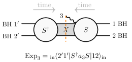
Figure 1: The KMOC momentum space waveform as the expectation value of measuring a graviton (labelled by $3$) in the background of two Schwarzschild black holes/heavy scalars (labelled by $1$ and $2$). The prime decorations on $1^{\prime}$ and $2^{\prime}$ emphasize that the scattering is non forward (no in and out states are exactly collinear). To obtain, e.g., the spectral waveform, one needs to Fourier transform this observable to impact parameter.

To establish the connection with scattering amplitudes more precisely, it is useful to first introduce the generators $a,a^{\dagger},b$ and $b^{\dagger}$ for the algebra of asymptotic measurements. Its existence is physically motivated by the naive expectation that finite energy excitations in the “bulk” should decay into a set of stable and free particles at asymptotic times. This means that the asymptotic states are assumed to be free of any external forces/fields, so that they do not radiate nor decay.

The annihilation and creation operators in the far past are denoted, respectively, by $a$ and $a^{\dagger}$, while those in the far future are similarly denoted by $b$ and $b^{\dagger}$. In what follows, the key property is that $a$ and $b$ are conjugated to each other with respect to unitary time evolution : $b=S^{\dagger}aS$ (and, similarly, $b^{\dagger}=S^{\dagger}a^{\dagger}S$), where $SS^{\dagger}=\mathbbm{1}$. We refer the reader to [59] for complementary details.

The background in which the scattering occurs is defined by perturbations of the time-invariant vacuum $|0\rangle$ in the far past

$$|12\rangle=a_{2}^{\dagger}a_{1}^{\dagger}|0\rangle\quad\text{and}\quad|1^{\prime}2^{\prime}\rangle=a_{2^{\prime}}^{\dagger}a_{1^{\prime}}^{\dagger}|0\rangle\,.$$ (38)

As these two-particle states evolve over time, they can interact non-trivially with each other (i.e., create and absorb particles). Then, $\text{Exp}_{3}$ is defined as

$$\text{Exp}_{3}={}_{\text{in}}\langle 2^{\prime}1^{\prime}|b_{3}|12\rangle_{\text{in}}\,.$$ (39)

The connection between $\text{Exp}_{3}$ and amplitudes is made manifest in two steps. First, using the relation $b=S^{\dagger}aS$ and inserting a complete basis of states $\mathbbm{1}=\operatorname*{\mathchoice{\ooalign{$\displaystyle\sum$\cr$\displaystyle\int$\cr}}{\ooalign{\raisebox{0.14pt}{\scalebox{0.7}{$\textstyle\sum$}}\cr$\textstyle\int$\cr}}{\ooalign{\raisebox{0.2pt}{\scalebox{0.6}{$\scriptstyle\sum$}}\cr$\scriptstyle\int$\cr}}{\ooalign{\raisebox{0.2pt}{\scalebox{0.6}{$\scriptstyle\sum$}}\cr$\scriptstyle\int$\cr}}}_{X}|X\rangle\langle X|$ in eq. (39), we obtain

$$\begin{split}\text{Exp}_{3}&={}_{\text{in}}\langle 2^{\prime}1^{\prime}|S^{\dagger}a_{3}S|12\rangle_{\text{in}}\\ &=\operatorname*{\mathchoice{\ooalign{$\displaystyle\sum$\cr$\displaystyle\int$\cr}}{\ooalign{\raisebox{0.14pt}{\scalebox{0.7}{$\textstyle\sum$}}\cr$\textstyle\int$\cr}}{\ooalign{\raisebox{0.2pt}{\scalebox{0.6}{$\scriptstyle\sum$}}\cr$\scriptstyle\int$\cr}}{\ooalign{\raisebox{0.2pt}{\scalebox{0.6}{$\scriptstyle\sum$}}\cr$\scriptstyle\int$\cr}}}_{X}{}_{\text{in}}\langle 2^{\prime}1^{\prime}|S^{\dagger}|X\rangle\langle X3|S|12\rangle_{\text{in}}\,.\end{split}$$ (40)

Next, plugging the decomposition formula $S=\mathbbm{1}+iT$ of the 4-point S-matrix (where $T$ is the connected part) into eq. (40), we obtain

$$\begin{split}\text{Exp}_{3}&={}_{\text{in}}\langle 32^{\prime}1^{\prime}|iT|12\rangle_{\text{in}}\\ &\qquad+\operatorname*{\mathchoice{\ooalign{$\displaystyle\sum$\cr$\displaystyle\int$\cr}}{\ooalign{\raisebox{0.14pt}{\scalebox{0.7}{$\textstyle\sum$}}\cr$\textstyle\int$\cr}}{\ooalign{\raisebox{0.2pt}{\scalebox{0.6}{$\scriptstyle\sum$}}\cr$\scriptstyle\int$\cr}}{\ooalign{\raisebox{0.2pt}{\scalebox{0.6}{$\scriptstyle\sum$}}\cr$\scriptstyle\int$\cr}}}_{X}{}_{\text{in}}\langle 2^{\prime}1^{\prime}|T^{\dagger}|X\rangle\langle X3|T|12\rangle_{\text{in}}\,.\end{split}$$ (41)

The first term is a (conventional) time-ordered $3\leftarrow 2$ amplitude, while the second term is a product of two time-ordered amplitudes glued together by a $s_{1^{\prime}2^{\prime}}=-(p_{1^{\prime}}{+}p_{2^{\prime}})^{2}$ channel cut. In practice, we can therefore compute $\text{Exp}_{3}$ perturbatively, directly from conventional time-ordered Feynman rules. (Alternatively, it was recently explained in [64] how to obtain such observables from analytic continuations of time-ordered scattering amplitudes.)

To eventually streamline comparison with experimental data, one may opt to work with waveforms expressed as functions of variables other than momenta. Such quantities can be derived from $\text{Exp}_{3}$ after performing additional Fourier transforms. For example, obtaining the spectral waveform requires to Fourier transform $\text{Exp}_{3}$ to impact parameter space. Similarly, to obtain the time domain waveform, an additional Fourier transform in the frequency of the outgoing graviton is needed.

It was recently demonstrated in [55] (see also [53]) that to obtain the leading-order (tree-level) spectral waveform in pure general relativity and $\mathcal{N}=8$ supergravity, one must perform Fourier transforms of the form

$$\begin{split}\mathcal{I}_{\beta_{1}\beta_{2}}^{\bm{\nu}_{2m}}&=\int_{\mathcal{M}}{\text{d}\bar{}\hskip 1.00006pt}^{\mathrm{D}}q\frac{\delta(u_{1}{\cdot}q)\delta(u_{2}{\cdot}(q{-}k))q^{\nu_{1}}{\dots}q^{\nu_{2m}}\mathrm{e}^{-iq\cdot b}}{[q^{2}-i\varepsilon]^{\beta_{1}}[(q{-}k)^{2}-i\varepsilon]^{\beta_{2}}}\,,\end{split}$$ (42)

where the $u_{i}$ s denote the (dimensionless) classical velocities of the heavy external objects, $k$ is the (on-shell: $k^{2}=0$) graviton momentum and $b$ the impact parameter.

In what follows, we showcase how our method can be applied to obtain new $\mathrm{D}$-dimensional closed form formulae for eq. (42) in the case where $\beta_{2}=0$. (Given that the ultra-soft graviton limits of the results presented below are not smooth, a separate evaluation of eq. (42) for $k^{\mu}=0$ is provided for completeness in app. C.)

Evaluation of $\mathcal{I}_{\beta_{1}0}^{\bm{\nu}_{2m}}$

The tensor reduction of eq. (42) is simple to perform. We find

$$\begin{split}\mathcal{I}_{\beta_{1}0}^{\bm{\nu}_{2m}}&=\mathcal{N}\leavevmode\nobreak\ \mathcal{I}_{\beta_{1}-m}\,,\end{split}$$ (43)

where we define

$$\mathcal{I}_{\alpha} =\int_{\mathcal{M}}{\text{d}\bar{}\hskip 1.00006pt}^{\mathrm{D}}q\frac{\delta(u_{1}{\cdot}q)\delta(u_{2}{\cdot}(q{-}k))\mathrm{e}^{-iq\cdot b}}{[q^{2}-i\varepsilon]^{\alpha}}\,,$$ (44a)

$$\mathcal{N} =\frac{(-1)^{m}\big{[}\eta^{\otimes m}\big{]}^{\{\bm{\nu}_{2m}\}}}{\prod_{j=1}^{m}(\mathrm{D}{+}2(m{-}1))}\,.$$ (44b)

Above, $\eta^{\otimes m}$ denotes $m$ occurrences of the metric tensor, $[\dots]^{\{\bm{\nu}_{2m}\}}$ stands for the sum over all possible shuffling of the $2m$ Lorentz indices $\nu_{i}$ in the tensor $[\dots]$.

Defining the kinematics as

$$u_{i}^{2} =-1\,, u_{1}\cdot u_{2} =-y\,, u_{i}\cdot b =0\,,$$ (45)

$$k\cdot b =0\,, k\cdot u_{1} =-w_{1}\,, k\cdot u_{2} =-w_{2}\,,$$

and denominators

$$z_{1}=u_{1}\cdot q\,,\leavevmode\nobreak\ z_{2}=u_{2}\cdot q+w_{2}\,,\leavevmode\nobreak\ z_{3}=q^{2}\,,\leavevmode\nobreak\ z_{4}=-ib\cdot q\,,$$ (46)

the integral in Baikov representation reads:

$$\mathcal{I}_{\alpha}=\int_{\mathcal{M}}\frac{\mathrm{d}\mathbf{z}}{z_{3}^{\alpha}}u(\mathbf{z})\delta(z_{1})\delta(z_{2})\,.$$ (47)

Treating the delta functions appearing as cut propagators, we can rewrite the integrals by taking the residues at $z_{1}=0$ and $z_{2}=0$ as

$$\mathcal{I}_{\alpha}=\int_{\mathcal{M}}\frac{\mathrm{d}\mathbf{z}}{z_{3}^{\alpha}}u(\mathbf{z})\big{|}_{z_{1}=z_{2}=0}\,,$$ (48)

where the twist on the cut is defined as

$$\begin{split}u(\mathbf{z})\big{|}_{z_{1}=z_{2}=0}&=-i\mathrm{e}^{z_{4}}\frac{\left(-b^{2}\left(y^{2}-1\right)\right)^{2-\frac{\mathrm{D}}{2}}}{2^{\frac{\mathrm{D}}{2}}\pi^{3/2}\Gamma\left(\frac{\mathrm{D}-3}{2}\right)}\\ &\times\left(b^{2}w_{2}^{2}-\left(y^{2}-1\right)\left(b^{2}z_{3}+z_{4}^{2}\right)\right)^{\frac{\mathrm{D}-5}{2}}\,.\end{split}$$ (49)

Rescaling with respect to $|b|$ allows us to work with dimensionless integrals $\mathcal{K}_{n}$ defined as

$$\mathcal{I}_{\alpha}=|b|^{2+2\alpha-\mathrm{D}}\mathcal{K}_{\alpha}\,.$$ (50)

We find $\nu=2$ master integrals, which we define as $\bm{\mathcal{K}}=\{\mathcal{K}_{1},\mathcal{K}_{2}\}$.

Next, defining the dimensionless parameter $s=w_{2}^{2}\,b^{2}$, intersection decompositions yield the system of differential equations

$$\partial_{s}\bm{\mathcal{K}} =\bm{\Omega}_{s}\cdot\bm{\mathcal{K}}\ ,\quad\quad\bm{\Omega}_{s}=\begin{pmatrix}0&\frac{-1}{y^{2}-1}\\ -\frac{1}{4s}&\frac{\mathrm{D}-6}{2s}\end{pmatrix}\,,$$ (51a)

$$\partial_{y}\bm{\mathcal{K}} =\bm{\Omega}_{y}\cdot\bm{\mathcal{K}}\ ,\quad\quad\bm{\Omega}_{y}=\begin{pmatrix}\frac{-y}{y^{2}-1}&\frac{2sy}{\left(y^{2}-1\right)^{2}}\\ \frac{y}{2\left(y^{2}-1\right)}&\frac{(5-\mathrm{D})y}{y^{2}-1}\end{pmatrix}\,.$$ (51b)

In terms of the dimensionful master integrals, the solution to eq. (51a) reads

$$\mathcal{I}_{1}=\left(b^{2}/w_{2}^{2}\right)^{\frac{4{-}\mathrm{D}}{4}}\left(y^{2}{-}1\right)^{\frac{2{-}\mathrm{D}}{4}}$$ (52)

$$\times\left[c_{1}I_{2-\frac{\mathrm{D}}{2}}\left(\frac{\sqrt{b^{2}}w_{2}}{\sqrt{y^{2}{-}1}}\right)-c_{2}I_{\frac{\mathrm{D}}{2}-2}\left(\frac{\sqrt{b^{2}}w_{2}}{\sqrt{y^{2}{-}1}}\right)\right]\,,$$

and similarly for $\mathcal{I}_{2}$. In this expression, $I_{\nu}(z)$ denotes the modified Bessel function of the first kind.

We now fix the boundary conditions. Similarly to what happened in eq. (31), in the neighborhood of $b^{2}=\infty$ approached from

$$b^{0}\to\begin{cases}i\infty&\text{for}\,q^{0}\geq 0\,,\\ -i\infty&\text{for}\,q^{0}<0\,,\end{cases}\quad\text{and fixed}\quad\mathbf{b}\,,$$ (53)

the integrand in eq. (44a) is exponentially suppressed (see eq. (32)) and thus vanishes. This condition fixes

$$c_{2}=c_{1}\,,$$ (54)

in eq. (52).

To fix $c_{1}$, we evaluate eq. (44a) at zero impact parameter. In doing so, it is convenient to commit to the rest frame of $u_{1}$, where

$$u_{1}=(1,0,\mathbf{0}_{\perp})\quad\text{and}\quad u_{2}=(y,\sqrt{y^{2}{-}1},\mathbf{0}_{\perp})\,,$$ (55)

such that $u_{1}{\cdot}u_{2}=-y$. In this frame, the integral at $b^{\mu}=0$ becomes

$$\begin{split}\mathcal{I}_{\alpha}|_{b=0}&=\int_{\mathcal{M}}{\text{d}\bar{}\hskip 1.00006pt}^{\mathrm{D}}q\frac{\delta(q^{0})\delta(yq^{0}{-}\sqrt{y^{2}{-}1}q^{1}{-}w_{2})}{[-(q^{0})^{2}+(q^{1})^{2}+(\mathbf{q}_{\perp})^{2}-i\varepsilon]^{\alpha}}\,.\end{split}$$ (56)

Integrating out the two delta functions gives the $\alpha^{\text{th}}$ mass derivative of the Euclidean $(\mathrm{D}{-}2)$-dimensional tadpole of mass $\mathfrak{m}=w_{2}/\sqrt{y^{2}-1}$

$$\mathcal{I}_{\alpha}|_{b=0} =\frac{1}{2\pi\sqrt{y^{2}{-}1}}\partial^{(\alpha)}_{\mathfrak{m}^{2}}\int_{\mathbbm{R}^{\mathrm{D}-2}}\frac{{\text{d}\bar{}\hskip 1.00006pt}^{\mathrm{D}-2}\mathbf{q}_{\perp}}{(\mathbf{q}_{\perp})^{2}+\mathfrak{m}^{2}}$$ (57)

$$=\frac{\Gamma(\alpha{+}1{-}\mathrm{D}/2)}{2^{\mathrm{D}/2}\pi\Gamma(\alpha)\sqrt{y^{2}{-}1}}\left[\frac{y^{2}{-}1}{w_{2}^{2}}\right]^{\alpha{+}1{-}\mathrm{D}/2}\,.$$

Using these results, and by computing the $b\to 0$ limit of eq. (52), $c_{1}$ is fixed to

$$c_{1}=\frac{1}{4}\csc\left(\frac{\pi\mathrm{D}}{2}\right)\,.$$ (58)

Putting everything together, the final expressions for the dimensionful master integrals read

$$\mathcal{I}_{1} =\frac{\left(b^{2}/w_{2}^{2}\right)^{\frac{4{-}\mathrm{D}}{4}}}{2\pi\left(y^{2}{-}1\right)^{\frac{\mathrm{D}{-}2}{4}}}K_{\frac{4{-}\mathrm{D}}{2}}\left(\frac{\sqrt{b^{2}}w_{2}}{\sqrt{y^{2}{-}1}}\right)\,,$$ (59a)

$$\mathcal{I}_{2} =\frac{\left(b^{2}/w_{2}^{2}\right)^{\frac{6{-}\mathrm{D}}{4}}}{4\pi\left(y^{2}{-}1\right)^{\frac{\mathrm{D}{-}4}{4}}}K_{\frac{6{-}\mathrm{D}}{2}}\left(\frac{\sqrt{b^{2}}w_{2}}{\sqrt{y^{2}-1}}\right)\,.$$ (59b)

where $K_{\nu}(z)$ stands for the modified Bessel function of the second kind. The $\mathrm{D}\to 4$ limit of eq. (59a) is smooth and agrees with [53, eq.  (C16)], once convention differences are taken into account. The $\mathrm{D}$-dimensional analytic expressions in eq. (59) are new and constitute one of the main results of this work.

III.3 QCD color dipole scattering

A central objective of future electron-ion collision experiments [65] is to gather data on how the density of partons inside hadrons changes as a function of energy. It is theorized that, as energy increases, this density becomes larger and larger until it reaches the so-called saturation regime of QCD, where non-linear effects from gluon recombination ($gg\to g$) take over soft bremsstrahlung. This prediction arises in the color glass condensate interpretation of deep inelastic scattering (DIS) [66, 67]. In this framework, the incoming lepton emits a high-energy virtual photon scattering from the color potential of the proton. This interaction is then modeled in the frame where the virtual photon fluctuates into a color dipole (quarkonia) that scatters eikonally from the color potential (see Fig. 2).

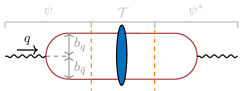
Figure 2: The bare color dipole cross-section discussed in the main text. The eikonal quark and anti-quark are represented by (red) Wilson lines. The color potential, which appears as a static two-dimensional pancake in the laboratory rest frame, models the highly boosted target nucleus and is represented by the blue region.

At leading order, the total cross-section for the photon polarization states is obtained by applying the optical theorem to the color dipole forward amplitude $\mathcal{T}$ [68]

$$\begin{split}\sigma^{\gamma^{\ast}p}_{\text{LO}}=2\int\text{d}^{2}\mathbf{b}_{q}\text{d}^{2}\mathbf{b}_{\bar{q}}\text{d}z&|\psi(\Delta_{\perp},q^{2},z)|^{2}\mathcal{T}(\mathbf{b}_{q},\mathbf{b}_{\bar{q}},Y)\,.\end{split}$$ (60)

Here, $\psi=\psi_{\gamma^{\ast}\uparrow q\bar{q}}$ denotes the lightcone wavefunction of the virtual photon of momentum $q$ in the frame where it decays into a quarkonia dipole of transverse size $\Delta_{\perp}{=}|\mathbf{b}_{q}{-}\mathbf{b}_{\bar{q}}|$ carrying a fraction $z$ of the photon’s longitudinal momentum. The forward amplitude $\mathcal{T}$ is related to the correlator of Wilson lines

$$\tilde{U}(\mathbf{b}_{q},\mathbf{b}_{\bar{q}},Y)=\frac{1}{N_{\text{c}}}\text{tr}[U(\mathbf{b}_{q},Y)U^{\dagger}(\mathbf{b}_{\bar{q}},Y)]\,,$$ (61)

via $\mathcal{T}=1-\tilde{U}$. Here, $N_{\text{c}}$ denotes the number of colors and each Wilson line $U(\mathbf{b}_{\mathfrak{p}},Y)$ represents a parton $\mathfrak{p}$ traversing the target at transverse position/impact parameter $\mathbf{b}_{\mathfrak{p}}$ and rapidity $Y=Y(z)$ (see Fig. 2).

The rapidity evolution of the target color field is described by the Jalilian-Marian–Iancu–McLerran–Weigert–Leonidov–Kovner (JIMWLK) equation [69]. An approximate, yet more tractable, large-$N_{\text{c}}$/mean-field description is given by the Balitsky–Kovchegov (BK) equation [70, 71, 72], which is to leading order accuracy given by

$$\begin{split}&\frac{\partial\tilde{U}(\mathbf{b}_{q},\mathbf{b}_{\bar{q}},Y)}{\partial Y}=\int\text{d}^{2}\mathbf{b}_{g}\leavevmode\nobreak\ \mathcal{K}_{\text{BK}}^{\text{LO}}(\mathbf{b}_{q},\mathbf{b}_{\bar{q}},\mathbf{b}_{g})\\ &\quad\times[\tilde{U}(\mathbf{b}_{q},\mathbf{b}_{g},Y)\tilde{U}(\mathbf{b}_{g},\mathbf{b}_{\bar{q}},Y)-\tilde{U}(\mathbf{b}_{q},\mathbf{b}_{\bar{q}},Y)]\,,\end{split}$$ (62)

where $\mathcal{K}_{\text{BK}}^{\text{LO}}(\mathbf{b}_{q},\mathbf{b}_{\bar{q}},\mathbf{b}_{g})=\frac{\alpha_{\text{s}}N_{\text{c}}}{2\pi^{2}}\frac{(\mathbf{b}_{\bar{q}}-\mathbf{b}_{q})^{2}}{(\mathbf{b}_{\bar{q}}-\mathbf{b}_{g})^{2}(\mathbf{b}_{q}-\mathbf{b}_{g})^{2}}$ and $\alpha_{\text{s}}$ is the strong coupling constant.

The solution to the BK equation predicts an interesting feature of the DIS total cross-section known as geometrical scaling [76]. This scaling is indicative of gluon saturation within the hadron in the Regge limit.

Over the past decade, significant efforts have been made to refine the BK equation by including next-to-leading order corrections and beyond (see, e.g., [77, 78, 79, 73]). These refinements involve calculating higher-order corrections in the strong coupling constant, which can be quite cumbersome. In particular, as intermediate steps, it is often necessary to trade the transverse-momentum dependence in expressions in favor of transverse position. This step necessarily leads to complicated Fourier integrals.

As illustrative examples, we consider two $\mathrm{D}$-dimensional families of integrals relevant to deep inelastic scattering in the saturation regime

$$I^{ij} =\int_{\mathbbm{R}^{2\mathrm{D}}}{\text{d}\bar{}\hskip 1.00006pt}^{\mathrm{D}}q_{1}{\text{d}\bar{}\hskip 1.00006pt}^{\mathrm{D}}q_{2}\frac{N_{I}^{ij}(q_{1},q_{2})\mathrm{e}^{i(q_{1}\cdot x_{1}{+}q_{2}\cdot x_{2})}}{q_{1}^{2}(q_{1}^{2}\tau{+}q_{2}^{2})}\,,$$ (63a)

$$G^{ij} =\int_{\mathbbm{R}^{2\mathrm{D}}}{\text{d}\bar{}\hskip 1.00006pt}^{\mathrm{D}}q_{1}{\text{d}\bar{}\hskip 1.00006pt}^{\mathrm{D}}q_{2}\frac{N_{G}^{ij}(q_{1},q_{2})\mathrm{e}^{i(q_{1}\cdot x_{1}+q_{2}\cdot x_{2})}}{(q_{1}+q_{2})^{2}(q_{1}^{2}\tau+q_{2}^{2})}\,,$$ (63b)

where the $q_{i}\equiv\mathbf{q}^{\perp}_{i}$s are Euclidean, $1\geq\tau>0$ and

$$\begin{split}N_{I}^{ij}&=q_{1}^{i}q_{2}^{j}\,,\\ N_{G}^{ij}&=\delta^{ij}(q_{1}^{2}{-}q_{2}^{2}){-}\frac{2q_{1}^{i}(q_{1}{+}q_{2})^{j}}{u}{+}\frac{2(q_{1}{+}q_{2})^{i}q_{2}^{j}}{u\tau}\,.\end{split}$$ (64)

In particular, in $\mathrm{D}=2$, eqs. 63a and 63b appear in the derivation of the NLO BK equation [77, eq. (42)]. A small subset of diagrams leading to their appearance is shown in Fig. 3.

In the following, we present new closed-form formulae for eqs. 63a and 63b in $\mathrm{D}$ dimensions. We anticipate these results to be useful considering that the $\mathcal{O}(\epsilon)$ correction to the NLO BK equation yields non-trivial contributions to the NNLO BK equation in the critical dimension.

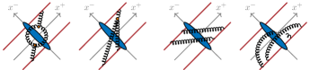
Figure 3: A small sample of NLO diagrams relevant to the rapidity evolution of a color dipole in lightcone coordinates (the transverse direction is left implicit). The first diagram exemplifies a cut self-energy correction, while the subsequent ones illustrate cut vertices. The Fourier integrals discussed in the main text emerge as intermediate steps in the computation of NLO BK observables in $\mathrm{D}$-dimensions.

Tensor decomposition

We first perform the tensor decomposition of $I^{ij}$ and $G^{ij}$, namely

$$I^{ij}=\sum_{a=1}^{5}I_{a}t_{a}^{ij}\quad\text{and}\quad G^{ij}=\sum_{a=1}^{5}G_{a}t_{a}^{ij}\,,$$ (65)

with basis

$$t_{1}^{ij}=x_{1}^{i}x_{1}^{j},\quad t_{2}^{ij} =x_{1}^{i}x_{2}^{j},\quad t_{3}^{ij}=x_{2}^{i}x_{1}^{j},$$ (66)

$$t_{4}^{ij}=x_{2}^{i}x_{2}^{j}, \quad t_{5}^{ij}=\delta^{ij}\,.$$

Here, $I_{a}$ and $G_{a}$ are respectively given by

$$\{I_{a},G_{a}\}=\sum_{b=1}^{5}(T^{-1})_{ab}\{K_{a}^{(I)},K^{(G)}_{a}\}\,,$$ (67)

where we have defined

$$K_{a}^{(I)}=t_{a}^{ij}I^{ij}\,,\quad K_{a}^{(G)}=t_{a}^{ij}I^{ij}\,,\quad T_{ab}=t_{a}^{ij}t_{b}^{ij}\,.$$ (68)

Therefore, in order to find the tensor decompsoition of these integrals, our first task is to compute the scalar integrals $K_{a}^{(I)}$ and $K_{a}^{(G)}$ for $a=1,\dots,5$.

Change of variables

For $K_{a}^{(I)}$, we make the change of variables

$$q_{1}=\frac{\kappa_{1}}{\sqrt{\tau}\absolutevalue{x_{2}}}\quad\text{and}\quad q_{2}=\frac{\kappa_{2}}{\absolutevalue{x_{2}}}\,,$$ (69)

while for $K_{a}^{(G)}$, we instead consider

$$q_{1}=\frac{\kappa_{1}-\sqrt{\tau}\kappa_{2}}{\sqrt{\tau}\absolutevalue{x_{2}-x_{1}}}\quad\text{and}\quad q_{2}=\frac{\sqrt{\tau}\kappa_{1}+\kappa_{2}}{\absolutevalue{x_{2}-x_{1}}}\,.$$ (70)

From there, we define the dimensionless vectors

$$\xi_{1}=\frac{x_{1}}{\sqrt{\tau}\absolutevalue{x_{2}}}, \quad\xi_{2}=\frac{x_{2}}{\absolutevalue{x_{2}}}\,,$$ (71a)

$$\zeta_{1}=\frac{x_{1}+\tau x_{2}}{\sqrt{\tau}\absolutevalue{x_{2}-x_{1}}}, \quad\zeta_{2}=\frac{x_{2}-x_{1}}{\absolutevalue{x_{2}-x_{1}}}\,,$$ (71b)

such that both integrals take the universal form

$$K_{a}^{(I)} =(\sqrt{\tau}x_{2}^{2})^{2-\mathrm{D}}\mathcal{I}\left(\xi_{1},\xi_{2};\mathcal{N}_{a}^{(I)}\right)\,,$$ (72a)

$$K_{a}^{(G)} =\frac{(1+\tau)^{\mathrm{D}-3}}{(\sqrt{\tau}(x_{2}-x_{1})^{2})^{\mathrm{D}-2}}\mathcal{I}\left(\zeta_{1},\zeta_{2};\mathcal{N}_{a}^{(G)}\right)\,,$$ (72b)

where

$$\mathcal{I}\left(\eta_{1},\eta_{2};\mathcal{N}\right)=\int_{\mathbbm{R}^{2\mathrm{D}}}{\text{d}\bar{}\hskip 1.00006pt}^{\mathrm{D}}\kappa_{1}{\text{d}\bar{}\hskip 1.00006pt}^{\mathrm{D}}\kappa_{2}\ \frac{\mathcal{N}\mathrm{e}^{i(\kappa_{1}\cdot\eta_{1}+\kappa_{2}\cdot\eta_{2})}}{\kappa_{1}^{2}(\kappa_{1}^{2}+\kappa_{2}^{2})}\,,$$ (73)

and $\eta_{2}^{2}=1$. The numerators are respectively given by

$$\mathcal{N}_{a}^{(I)} =t_{a}^{ij}N_{I}^{ij}\left(\frac{\kappa_{1}}{\sqrt{\tau}\absolutevalue{x_{2}}},\frac{\kappa_{2}}{\absolutevalue{x_{2}}}\right)\,,$$ (74a)

$$\mathcal{N}_{a}^{(G)} =t_{a}^{ij}N_{G}^{ij}\left(\frac{\kappa_{1}-\sqrt{\tau}\kappa_{2}}{\sqrt{\tau}\absolutevalue{x_{2}-x_{1}}},\frac{\sqrt{\tau}\kappa_{1}+\kappa_{2}}{\absolutevalue{x_{2}-x_{1}}}\right)\,.$$ (74b)

Master integrals of $\mathcal{I}$

In Baikov representation, the family of integrals defined in eq. (73) reads

$$\mathcal{I}(\eta_{1},\eta_{2};\mathcal{N})=\int_{C_{R}}\mathrm{d}^{7}\mathbf{z}\frac{u(\mathbf{z})f(\mathbf{z})}{z_{1}z_{2}}\,,$$ (75)

where $z_{1}=\kappa_{1}^{2}$, $z_{2}=\kappa_{1}^{2}+\kappa_{2}^{2}$, $z_{3}=\kappa_{1}\cdot\kappa_{2}$, $z_{4}=\kappa_{1}\cdot\eta_{1}$, $z_{5}=\kappa_{1}\cdot\eta_{2}$, $z_{6}=\kappa_{2}\cdot\eta_{1}$, $z_{7}=\kappa_{2}\cdot\eta_{2}$, and only $z_{1}$ and $z_{2}$ can appear as denominators. The twist is given by

$$u(\mathbf{z})=-\frac{\mathrm{e}^{i(z_{4}+z_{7})}(\eta_{1}^{2}-(\eta_{1}\cdot\eta_{2})^{2})^{\frac{3-\mathrm{D}}{2}}}{2^{\mathrm{D}}\pi^{5/2}\Gamma((\mathrm{D}{-}3)/2)\Gamma(\mathrm{D}/2{-}1)}B(\mathbf{z})^{\frac{\mathrm{D}-5}{2}}\,,$$ (76)

where $B(\mathbf{z})$ is given in the ancillary file and $f(\mathbf{z}(\kappa_{1},\kappa_{2},\eta_{1},\eta_{2}))=\mathcal{N}$. In this case, there are two master integrals

$$J_{1}(\eta_{1},\eta_{2}) =\mathcal{I}(\eta_{1},\eta_{2};\kappa_{1}^{2})=\int_{C_{R}}\mathrm{d}^{7}\mathbf{z}\frac{u(\mathbf{z})}{z_{2}}\,,$$ (77a)

$$\frac{J_{2}(\eta_{1},\eta_{2})}{(\mathrm{D}-2)^{2}} =\mathcal{I}(\eta_{1},\eta_{2};1)=\int_{C_{R}}\mathrm{d}^{7}\mathbf{z}\frac{u(\mathbf{z})}{z_{1}z_{2}}\,,$$ (77b)

where the factor $(\mathrm{D}-2)^{2}$ is introduced for later convenience.

Using intersection decompositions, the differential equations for the basis $\mathbf{J}=(J_{1},J_{2})^{T}$ read

$$\partial_{\eta_{1}^{2}}\mathbf{J} =\bm{\Omega}_{\eta_{1}^{2}}\cdot\mathbf{J},\quad\bm{\Omega}_{\eta_{1}^{2}}=\begin{pmatrix}\frac{1-\mathrm{D}}{1+\eta_{1}^{2}}&0\\ \frac{(\mathrm{D}-2)(1+\eta_{1}^{2})}{4\eta_{1}^{2}}&\frac{2-\mathrm{D}}{2\eta_{1}^{2}}\end{pmatrix}\,,$$ (78)

$$\partial_{\eta_{1}\cdot\eta_{2}}\mathbf{J} =\mathbf{0}\,.$$

The solutions to this system of differential equations is

$$J_{1}(\eta_{1}) =J_{10}(1+\eta_{1}^{2})^{1-\mathrm{D}}\,,$$ (79a)

$$J_{2}(\eta_{1}) =J_{20}(\eta_{1}^{2})^{\frac{2{-}\mathrm{D}}{2}}{+}\frac{J_{10}}{2}\mathcal{F}^{(I)}\,,$$ (79b)

with $\mathcal{F}^{(I)}={}_{2}F_{1}\left(\frac{\mathrm{D}{-}2}{2},\mathrm{D}{-}2,\frac{\mathrm{D}}{2},-\eta_{1}^{2}\right)$.

To fix the constants $J_{10}$ and $J_{20}$, we examine the boundary conditions at $\eta_{1}=0$. For $\mathbf{J}$, the limits evaluate to

$$J_{1}(0) =2^{\mathrm{D}-2}\Gamma(\mathrm{D}-1)\,,$$ (80a)

$$J_{2}(0) =2^{\mathrm{D}-3}\Gamma(\mathrm{D}-1)\,,$$ (80b)

as shown in app. D. Thus, since eq. (79) yields $J_{1}(0)=J_{10}$, we immediately see that

$$J_{10} =2^{\mathrm{D}-2}\Gamma(\mathrm{D}-1)\,.$$ (81)

To fix $J_{20}$ we use the fact that $J_{2}(0)$ is finite. This necessarily requires $J_{20}=0$.

Computing $I^{ij}$

For $I^{ij}$, we have that $\eta_{1}=\xi_{1}$ and $\eta_{2}=\xi_{2}$. Thus, the master integrals are

$$J_{1}^{(I)} =2^{\mathrm{D}-2}\Gamma(\mathrm{D}-1)\left(1+\frac{x_{1}^{2}}{\tau x_{2}^{2}}\right)^{1-\mathrm{D}}\,,$$ (82a)

$$J_{2}^{(I)} =2^{\mathrm{D}-3}\Gamma(\mathrm{D}-1)\mathcal{F}^{(I)}\,,$$ (82b)

with $\mathcal{F}^{(I)}={}_{2}F_{1}\left(\frac{\mathrm{D}-2}{2},\mathrm{D}-2,\frac{\mathrm{D}}{2},-\frac{x_{1}^{2}}{\tau x_{2}^{2}}\right)$.

We can then decompose the $\mathcal{I}$ integrals in eq. (73) in terms of these master integrals to find

$$K^{(I)}_{1} =\frac{\sqrt{\tau}x_{12}\mathcal{J}}{(\sqrt{\tau}x_{2}^{2})^{\mathrm{D}-1}},\quad K^{(I)}_{2}=\frac{\mathcal{J}}{(\sqrt{\tau}x_{2}^{2})^{\mathrm{D}-2}}\,,$$ (83a)

$$K^{(I)}_{3} =\frac{\sqrt{\tau}x_{12}^{2}\mathcal{J}}{x_{1}^{2}(\sqrt{\tau}x_{2}^{2})^{\mathrm{D}-1}},\quad K^{(I)}_{4}=\frac{x_{12}\mathcal{J}}{x_{1}^{2}(\sqrt{\tau}x_{2}^{2})^{\mathrm{D}-2}}\,,$$ (83b)

$$K^{(I)}_{5} =\frac{\sqrt{\tau}x_{12}\mathcal{J}}{x_{1}^{2}(\sqrt{\tau}x_{2}^{2})^{\mathrm{D}-1}}\,,$$ (83c)

where $x_{12}=x_{1}\cdot x_{2}$ and $\mathcal{J}=\left(\frac{\tau x_{2}^{2}-x_{1}^{2}}{2\tau x_{2}^{2}}J_{1}^{(I)}-J_{2}^{(I)}\right)$.

Applying the transformation described earlier in eq. (67), we find

$$I_{1}=I_{3}=I_{4}=I_{5}=0\quad\text{and}\quad I_{2}=\frac{\sqrt{\tau}\mathcal{J}}{x_{1}^{2}(\sqrt{\tau}x_{2}^{2})^{\mathrm{D}-1}}\,.$$ (84)

The final answer is then

$$I^{ij}=\frac{\sqrt{\tau}\mathcal{J}x_{1}^{i}x_{2}^{j}}{x_{1}^{2}(\sqrt{\tau}x_{2}^{2})^{\mathrm{D}-1}}\,.$$ (85)

In $\mathrm{D}=2$, we find

$$I^{ij}=-\frac{x_{1}^{i}x_{2}^{j}}{x_{2}^{2}(x_{1}^{2}+\tau x_{2}^{2})}\,,$$ (86)

in agreement with the known result given in [77, eq. (42)]. (Subleading terms in the $\mathrm{D}=2-2\epsilon$ expansion are provided in app. E for ‘QCD practitioners’ convenience.)

Computing $G^{ij}$

For $G^{ij}$, we have instead that $\eta_{1}=\zeta_{1}$ and $\eta_{2}=\zeta_{2}$. Thus, the master integrals are

$$J_{1}^{(G)} =2^{\mathrm{D}-2}\Gamma(\mathrm{D}-1)\left(\frac{(1+\tau)(x_{1}^{2}+\tau x_{2}^{2})}{\tau(x_{2}-x_{1})^{2}}\right)^{1-\mathrm{D}}\,,$$ (87a)

$$J_{2}^{(G)} =2^{\mathrm{D}-3}\Gamma(\mathrm{D}-1)\mathcal{F}^{(G)}\,,$$ (87b)

with $\mathcal{F}^{(G)}={}_{2}F_{1}\left(\frac{\mathrm{D}-2}{2},\mathrm{D}-2,\frac{\mathrm{D}}{2},-\frac{(x_{1}+\tau x_{2})^{2}}{\tau(x_{2}-x_{1})^{2}}\right)$.

We again decompose our integrals and transform back to our tensor decomposition in eq. (67) to find

$$G_{1} =\frac{(1+\tau)^{\mathrm{D}-1}\left(Y_{1}J_{1}^{(G)}+2\tau(x_{2}-x_{1})^{2}J_{2}^{(G)}\right)}{u\tau^{1+\frac{\mathrm{D}}{2}}(x_{1}+\tau x_{2})^{2}((x_{2}-x_{1})^{2})^{\mathrm{D}}}\,,$$ (88)

$$G_{2} =(\tau-1)G_{1}\,,\quad G_{3}=0\,,\quad G_{4}=-\tau G_{1}\,,$$

$$G_{5} =-\frac{(1+\tau)^{\mathrm{D}-2}\left(Y_{2}J_{1}^{(G)}+Y_{3}J_{2}^{(G)}\right)}{\tau^{\frac{\mathrm{D}}{2}}(x_{1}+\tau x_{2})^{2}((x_{2}-x_{1})^{2})^{\mathrm{D}}}\,,$$

where

$$Y_{1} =4\tau x_{12}+(\tau-1)(\tau x_{2}^{2}-x_{1}^{2})\,,$$ (89a)

$$Y_{2} =(1+\tau)^{2}((\tau-1)x_{1}^{2}x_{2}^{2}+(x_{1}^{2}-\tau x_{2}^{2})x_{12})\,,$$ (89b)

$$Y_{3} =2\tau(x_{2}-x_{1})^{2}((\tau-1)x_{12}+x_{1}^{2}-\tau x_{2}^{2}))\,.$$ (89c)

The final result is then given by eq. (65) and reads

$$G^{ij}=\sum_{a=1}^{5}G_{a}t_{a}^{ij}\,.$$ (90)

In $\mathrm{D}=2$, we find that

$$G^{ij}=\frac{2\tau(x_{1}{-}x_{2})^{i}x_{2}^{j}{+}2x_{1}^{i}(x_{1}{-}x_{2})^{j}{+}u\tau(x_{2}^{2}{-}x_{1}^{2})\delta^{ij}}{u\tau(x_{2}{-}x_{1})^{2}(x_{1}^{2}{+}\tau x_{2}^{2})}\,,$$ (91)

which is also in agreement with [77]. (Once again, subleading terms in the $\epsilon$-expansion are provided in app. E.)

Let us close this application by noting that for both eqs. 85 and 90, the $\epsilon$-expansions (see app. E) involve only polylogarithms with rational coefficients in the kinematics. This observation resonates with the fact that the known results for NNLO BK in $\mathcal{N}=4$ super Yang-Mills involve only (weight three) polylogarithms with similar coefficients [73]. Therefore, one might naively expect the full QCD result to be constructed from similar functions.

The differential equation matrices evaluated in applications III.1, III.2 and III.3 by means of intersection numbers, have also been verified by computing integration-by-parts identities in momentum space.

IV Conclusions

In this letter, we applied intersection theory to dimensionally regularized Fourier integrals, extending the range of applicability of this technique in particle physics beyond Feynman integrals.

We showed how to express Fourier integrals as twisted periods by deriving their Baikov representation. From there, we explained how to derive relations between Fourier integrals within a given family and how to obtain the system of differential equations they satisfy using intersection numbers. This offered a fresh perspective on Fourier calculus, inspired by recent advances in Feynman calculus.

We showcased our method by computing explicitly relevant instances of Fourier integrals appearing in the tree-level spectral waveform within pure general relativity and $\mathcal{N}=8$ supergravity, as well as in color dipole scattering at next-to-leading order (NLO) in QCD. Each time, we were able to verify our new (dimensionally regularized) results with existing data from the literature in specific limits, highlighting the method’s accuracy and potential. We hope that these developments open up a number of new directions, some of which are outlined below.

It would be interesting to see to what extent the method described in this letter proves efficient in tackling the remaining integrals relevant to the tree-level spectral waveform (i.e., those with $\beta_{2}\neq 0$ in eq. (42)), and more ambitiously, those pertinent to the one-loop spectral waveform (these come with an additional loop integration on top of the impact parameter Fourier transform). To the authors’ knowledge, none of these has been analytically computed in $\mathrm{D}$ dimensions.

Similarly, it would also be interesting to investigate the extent to which our approach can be adapted to address the remaining steps in calculating the full NLO evolution of color dipoles within dimensional regularization (with or without the incorporation of running coupling corrections [83, 77]; the latter requiring the computation of Fourier transforms involving additional logarithms [83]). As stressed in the main text, such NLO results would contain valuable non-trivial information about higher-order corrections to the rapidity evolution equation in critical dimension, which is relevant for the phenomenology of high-energy hadronic and nuclear content.

From the mathematical point of view, the study of the cohomology of Fourier integrals, poses interesting questions on the type of systems of differential equations they obey, as well as on the type of functions that are expected to appear in their solutions, possibly involving new types of transcendental leading singularities/maximal cuts. Finally, it would be interesting to explore the extent to which tropical geometry [84, 85, 86, 87, 88] could be used in the context of Fourier integrals, offering new directions for their analytic and numerical evaluation.

Appendix A Derivation of the Baikov representation for Fourier integrals

Let us consider the generic Fourier integral given by eq. (17). To derive the Baikov representation, we first split each momentum $q_{j}$ into components perpendicular and parallel to the subspace spanned by $\{q_{j+1},\dots,q_{L},y_{1},\dots,y_{E}\}$. The effect on the measure is

$$\mathrm{d}^{\mathrm{D}}q_{j}=\mathrm{d}^{E-L-j}q_{j\parallel}\wedge\mathrm{d}^{\mathrm{D}-E+L+j}q_{j\bot}\,.$$ (92)

The parallel component gives

$$\mathrm{d}^{E-L-j}q_{j\parallel}=\frac{\bigwedge_{k=j+1}^{L}\mathrm{d}(q_{j}\cdot q_{k})\wedge\mathrm{d}(q_{j}\cdot y_{E})}{G^{1/2}(q_{j+1},\dots,q_{L},y_{1},\dots,y_{E})}\,,$$ (93)

while the perpendicular component gives (in spherical coordinates)

$$\mathrm{d}^{N}q_{j\bot} =q_{j\bot}^{N-1}\mathrm{d}\Omega_{N-2}\wedge\mathrm{d}q_{j\bot}$$

$$=\frac{1}{2}q_{j\bot}^{N-2}\mathrm{d}\Omega_{N-2}\wedge\mathrm{d}(q_{j\bot}^{2})$$ (94)

$$=\frac{1}{2}\left(\frac{G(q_{j},\dots,y_{E})}{G(q_{j+1},\dots,y_{E})}\right)^{\frac{N-2}{2}}\mathrm{d}\Omega_{N-2}\wedge\mathrm{d}(q_{j\bot}^{2})\,,$$

where $N=\mathrm{D}-E+L+j$ and $\mathrm{d}\Omega_{N-2}$ is the measure accounting for the $N-2$ angular degrees of freedom. Substituting eqs. 93 and 94 into eq. (92), we observe that the Gram determinants simplify, leading to

$$\int_{\mathbbm{R}^{L\mathrm{D}}}\prod_{j=1}^{L}{\text{d}\bar{}\hskip 1.00006pt}^{\mathrm{D}}q_{j} =\frac{\pi^{-\frac{L(L-1)}{4}-\frac{LE}{2}}G(y_{1},\dots,y_{E})^{\frac{-\mathrm{D}+E+1}{2}}}{2^{\frac{L\mathrm{D}}{2}}\prod_{j=1}^{L}\Gamma\left(\frac{\mathrm{D}-L-E+j}{2}\right)}$$

$$\times\int_{\mathbbm{R}^{n}}G(q_{1},\dots,y_{E})^{\frac{\mathrm{D}-L-E-1}{2}}\prod_{j=1}^{n}\mathrm{d}S_{j}\,.$$ (95)

We then conveniently redefine our propagators such that

$$z_{i}=A_{ij}S_{j}+B_{j}\,,$$ (96)

which introduces a Jacobian for the change of variables, given by $\det A$. Thus, we find

$$\int_{\mathbbm{R}^{L\mathrm{D}}}\prod_{j=1}^{L}{\text{d}\bar{}\hskip 1.00006pt}^{\mathrm{D}}q_{j}=\kappa\int_{\mathbbm{R}^{n}}\mathrm{d}^{n}\mathbf{z}B(\mathbf{z})^{(\mathrm{D}-L-E-1)/2}\,,$$ (97)

where $\kappa$ and $B(\mathbf{z})$ are defined in eqs. 23c and 23b, respectively.

Appendix B Fourier transform of a power-law

From the generalized Schwinger trick, we have

$$\begin{split}\int_{\mathbbm{R}^{\mathrm{D}}}{\text{d}\bar{}\hskip 1.00006pt}^{\mathrm{D}}q\frac{\mathrm{e}^{iq\cdot x}}{A(q)^{n}}&=\frac{2\pi^{n/2}}{\Gamma(n/2)}\int_{\mathbbm{R}^{\mathrm{D}}}{\text{d}\bar{}\hskip 1.00006pt}^{\mathrm{D}}q\leavevmode\nobreak\ \mathrm{e}^{iq\cdot x}\\ &\quad\times\int_{0}^{\infty}\mathrm{d}\xi\leavevmode\nobreak\ \xi^{n-1}\mathrm{e}^{-\pi\xi^{2}A(q)^{2}}\,.\end{split}$$ (98)

For $A(q)=q$, and after swapping the order of integration on the right-hand side, the inner integral becomes much easier to perform. This is because the Fourier transform of a Gaußian is itself a Gaußian

$$\int_{\mathbbm{R}^{\mathrm{D}}}{\text{d}\bar{}\hskip 1.00006pt}^{\mathrm{D}}q\leavevmode\nobreak\ \mathrm{e}^{-\pi\xi^{2}q^{2}}\mathrm{e}^{iq\cdot x}=\frac{\xi^{-\mathrm{D}}\mathrm{e}^{-\frac{x^{2}}{4\pi\xi^{2}}}}{(2\pi)^{\mathrm{D}/2}}\,.$$ (99)

Plugging this into eq. (98), we find (for $0<n<\mathrm{D}$)

$$\begin{split}\eqref{eq:todo0}|_{A=q}&=N\int_{0}^{\infty}\mathrm{d}\xi\xi^{n{-}\mathrm{D}{-}1}\mathrm{e}^{-\frac{x^{2}}{4\pi\xi^{2}}}\\ &=N\int_{0}^{\infty}\mathrm{d}\zeta\zeta^{(\mathrm{D}-n)-1}\mathrm{e}^{-\frac{x^{2}\zeta^{2}}{4\pi}}\\ &=\frac{\Gamma((\mathrm{D}-n)/2)}{2^{n-\mathrm{D}/2}\Gamma(n/2)}(x^{2})^{\frac{n-\mathrm{D}}{2}}\,,\end{split}$$ (100)

where $N=\frac{2\pi^{n/2}}{(2\pi)^{\mathrm{D}/2}\Gamma(n/2)}$ and $\zeta=1/\xi$. After a trivial change of variables, eq. (100) is seen to agree with [89, eq. (A.1)].

Appendix C Ultra-soft graviton spectral waveform

As complementary material to the results presented in sec. III.1, we examine the integral in eq. (42) in the ultra-soft graviton ($k^{\mu}=0$) regime

$$I_{\alpha}^{\mu}=\int_{\mathcal{M}}{\text{d}\bar{}\hskip 1.00006pt}^{\mathrm{D}}q\delta(u_{1}\cdot q) \delta(u_{2}\cdot q)\frac{\mathrm{e}^{-iq\cdot b}q^{\mu}}{(q^{2})^{\alpha}}\,,$$ (101)

using intersection theory and differential equations. This integral, while solvable through more conventional methods such as Schwinger parameters, remains a simple enough example to showcase the application of the techniques used to address the more challenging calculations discussed in the main text.

Evaluation of $I_{\alpha}^{\mu}$

We have $L=1$ internal vector $\{q\}$ and $E=3$ external vectors $\{b,u_{1},u_{2}\}$, with kinematics $u_{1}^{2}=u_{2}^{2}=-1$, $u_{1}\cdot u_{2}=-y$, $u_{1}\cdot b=u_{2}\cdot b=0$. We define the $n=4$ integration variables such that $z_{1}=q^{2}$, $z_{2}=-iq\cdot b$, $z_{3}=u_{1}\cdot q$ and $z_{4}=u_{2}\cdot q$.

By performing a tensor decomposition, the integral takes the form

$$I_{\alpha}^{\mu}=I_{\alpha}^{(1)}b^{\mu}+I_{\alpha}^{(2)}u_{1}^{\mu}+I_{\alpha}^{(3)}u_{2}^{\mu}\,.$$ (102)

It is easy to see from eq. (101) that contractions with $u_{1}$ or $u_{2}$ vanish due to the delta functions. Moreover, $u_{1}$ and $u_{2}$ are, by definition, transverse to the impact parameter $b$. Put together, these conditions give

$$0=I_{\alpha}^{(2)}+yI_{\alpha}^{(3)}=yI_{\alpha}^{(2)}+I_{\alpha}^{(3)}\,.$$ (103)

and thus $I_{\alpha}^{(2)}=I_{\alpha}^{(3)}=0$. This implies

$$I_{\alpha}^{\mu}=I_{\alpha}^{(1)}b^{\mu}=\frac{b_{\nu}I_{\alpha}^{\nu}}{b^{2}}b^{\mu}\,,$$ (104)

such that only $I_{\alpha}^{(1)}$ needs to be computed. Its Baikov representation takes the form

$$I_{\alpha}^{(1)}=\frac{1}{b^{2}}\int\mathrm{d}^{4}\mathbf{z}\,\frac{i\,z_{2}}{z_{1}^{\alpha}}u(\mathbf{z})\delta(z_{3})\delta(z_{4})\,,$$ (105)

where the twist reads

$$u(\mathbf{z})=-i\frac{\left(-b^{2}\left(y^{2}-1\right)\right)^{2-\frac{\mathrm{D}}{2}}}{2^{\mathrm{D}/2}\pi^{3/2}\Gamma\left(\frac{\mathrm{D}-3}{2}\right)}\times$$ (106)

$$\left(b^{2}\left(-\left(y^{2}-1\right)z_{1}-2yz_{4}z_{3}+z_{3}^{2}+z_{4}^{2}\right)-\left(y^{2}-1\right)z_{2}^{2}\right){}^{\frac{\mathrm{D}-5}{2}}\,.$$

We can then integrate out $z_{3}$ and $z_{4}$ using the delta functions to find

$$I_{\alpha}^{(1)}=\frac{1}{b^{2}}\int\mathrm{d}z_{1}\mathrm{d}z_{2}\frac{i\,z_{2}}{z_{1}^{\alpha}}u(z_{1},z_{2},0,0)\,.$$ (107)

There is only one master integral ($\nu{=}1$), defined as

$$J=\int{\text{d}\bar{}\hskip 1.00006pt}^{\mathrm{D}}q\delta(u_{1}\cdot q)\delta(u_{2}\cdot q)\frac{\mathrm{e}^{-iq\cdot b}}{q^{2}}\,.$$ (108)

$I_{\alpha}^{(1)}$ can then be decomposed onto this basis as

$$I_{\alpha}^{(1)}=\frac{i(4-\mathrm{D})}{b^{2}}J\,.$$ (109)

The master integral $J$ obeys the differential equations

$$\partial_{b^{2}}J=\frac{4{-}\mathrm{D}}{2b^{2}}J\quad\text{and}\quad\partial_{y}J=\frac{-y}{y^{2}{-}1}J\,.$$ (110)

The solution to these equations is easily seen to be

$$J=J_{0}\frac{(b^{2})^{(4-\mathrm{D})/2}}{\sqrt{y^{2}-1}}\,.$$ (111)

To fix the boundary constant $J_{0}$ a direct evaluation of $J$ in eq. (108) is performed at $b^{2}=1$: first, the two delta functions in the rest frame of $u_{2}$ are integrated over. Up to a normalization factor, this gives an Euclidean $(\mathrm{D}{-}2)$-dimensional tadpole integral with numerator $\mathrm{e}^{-iq\cdot b}$. After mapping this result back to Schwinger parameter space, the integral can be easily evaluated for $b^{2}=1$, similarly to the computation outlined in app. B. This allows us to fix

$$J_{0}=-\frac{i2^{\frac{\mathrm{D}}{2}}}{32}\Gamma(\mathrm{D}/2-2)\,.$$ (112)

Putting everything together, we obtain

$$I_{\alpha}^{\mu}=i(4-\mathrm{D})J_{0}\frac{(b^{2})^{(2-\mathrm{D})/2}}{\sqrt{y^{2}-1}}q^{\mu}\,.$$ (113)

Appendix D Boundary conditions for application III.3

We examine the $\eta_{1}=0$ limit of the master integrals in III.3

$$J_{1}(\eta_{1})=\mathcal{I}(\eta_{1},\eta_{2};\kappa_{1}^{2}),\quad J_{2}(\eta_{1})=\mathcal{I}(\eta_{1},\eta_{2};1)\,,$$ (114)

with $\mathcal{I}(\eta_{1},\eta_{2},\mathcal{N})$ being the family of integrals defined in eq. (73). If we set $\eta_{1}=0$, we have for the first master integral

$$J_{1}(0) =\int_{\mathbb{R}^{\mathrm{D}}}{\text{d}\bar{}\hskip 1.00006pt}^{\mathrm{D}}\kappa_{2}\mathrm{e}^{i\kappa_{2}\cdot\eta_{2}}\int_{\mathbb{R}^{\mathrm{D}}}\frac{{\text{d}\bar{}\hskip 1.00006pt}^{\mathrm{D}}\kappa_{1}}{\kappa_{1}^{2}+\kappa_{2}^{2}}$$

$$=\frac{\Gamma\left(1-\frac{\mathrm{D}}{2}\right)}{2^{\frac{\mathrm{D}}{2}}}\int_{\mathbb{R}^{\mathrm{D}}}{\text{d}\bar{}\hskip 1.00006pt}^{\mathrm{D}}\kappa_{2}\frac{\mathrm{e}^{i\kappa_{2}\cdot\eta_{2}}}{(\kappa_{2}^{2})^{1-\frac{\mathrm{D}}{2}}}$$

$$=2^{\mathrm{D}-2}\Gamma(\mathrm{D}-1)\,.$$ (115)

For the second master integral we have

$$\frac{J_{2}(0)}{(\mathrm{D}-2)^{2}}=\int_{\mathbb{R}^{\mathrm{D}}}{\text{d}\bar{}\hskip 1.00006pt}^{\mathrm{D}}\kappa_{2}\mathrm{e}^{i\kappa_{2}\cdot\eta_{2}}\int_{\mathbb{R}^{\mathrm{D}}}\frac{{\text{d}\bar{}\hskip 1.00006pt}^{\mathrm{D}}\kappa_{1}}{\kappa_{1}^{2}(\kappa_{1}^{2}+\kappa_{2}^{2})}$$

$$=\int_{\mathbb{R}^{\mathrm{D}}}{\text{d}\bar{}\hskip 1.00006pt}^{\mathrm{D}}\kappa_{2}\mathrm{e}^{i\kappa_{2}\cdot\eta_{2}}\int_{0}^{1}\mathrm{d}x\int_{\mathbb{R}^{\mathrm{D}}}\frac{{\text{d}\bar{}\hskip 1.00006pt}^{\mathrm{D}}\kappa_{1}}{(\kappa_{1}^{2}+\kappa_{2}^{2}x)^{2}}$$

$$=\frac{\Gamma\left(2-\frac{\mathrm{D}}{2}\right)}{2^{\frac{\mathrm{D}}{2}}}\int_{\mathbb{R}^{\mathrm{D}}}{\text{d}\bar{}\hskip 1.00006pt}^{\mathrm{D}}\kappa_{2}\frac{\mathrm{e}^{i\kappa_{2}\cdot\eta_{2}}}{(\kappa_{2}^{2})^{2-\frac{\mathrm{D}}{2}}}\times\left(\int_{0}^{1}\mathrm{d}xx^{\frac{\mathrm{D}}{2}-2}\right)$$

$$=\frac{2^{\mathrm{D}-3}\Gamma(\mathrm{D}-1)}{(\mathrm{D}-2)^{2}}\,.$$ (116)

In order to find these boundary conditions, we have used the result from [49, eq.(7.85)], the result from app. B, Feynman parameters.

Appendix E $\epsilon$-expansions for application III.3

In this appendix, we provide explicit formulae for the $\epsilon$-expansions of eqs. 85 and 90 up to $\mathcal{O}(\epsilon^{2})$, namely

$$\{I^{ij},G^{ij}\}=\sum_{n=0}^{2}\epsilon^{n}\big{\{}I^{ij}_{(n)},G^{ij}_{(n)}\big{\}}+\mathcal{O}(\epsilon^{3})\,.$$ (117)

The coefficients $I^{ij}_{(n)}$ are recorded explicitly in the text below, as well as in a computer-friendly form in the ancillary file ancillary.m. The coefficients $G^{ij}_{(n)}$ are much larger and, therefore, are only recorded in ancillary.m.

For the former, setting $I^{ij}_{(n)}=x_{1}^{i}x_{2}^{j}I_{(n)}$, we have

$$I_{(0)} =\eqref{eq:ILO}\,,$$ (118a)

$$I_{(1)} =\frac{\Delta_{-}\log\left[\tfrac{\tau x_{2}^{2}}{\Delta_{+}}\right]{-}2x_{1}^{2}\left(\log\left[\tfrac{\sqrt{\tau}x_{2}^{2}}{2}\right]{+}\gamma_{\text{E}}\right)}{\Delta_{+}x_{1}^{2}x_{2}^{2}}\,,$$ (118b)

$$I_{(2)} =\Big{[}3\Delta_{-}\log\left[\tfrac{\Delta_{+}}{\tau x_{2}^{2}}\right]\left(\log\left[\tfrac{\Delta_{+}}{\tau x_{2}^{2}}\right]{+}2\left(\log\left[\tfrac{\sqrt{\tau}x_{2}^{2}}{2}\right]{+}\gamma_{\text{E}}\right)\right)$$

$${+}3\Delta_{+}\text{Li}_{2}\left[\tfrac{-x_{1}^{2}}{\tau x_{2}^{2}}\right]{+}6x_{1}^{2}\left(\log\left[\tfrac{\sqrt{\tau}x_{2}^{2}}{4}\right]{+}2\gamma_{\text{E}}\right)\log\left[\sqrt{\tau}x_{2}^{2}\right]$$

$$+x_{1}^{2}\left(\pi^{2}+6(\gamma_{\text{E}}{-}\log 2)^{2}\right)\Big{]}/(3\Delta_{+}x_{1}^{2}x_{2}^{2})\,,$$ (118c)

where $\Delta_{\pm}=x_{1}^{2}\pm\tau x_{2}^{2}$.

References

- Chetyrkin and Tkachov [1981] K. G. Chetyrkin and F. V. Tkachov, Integration by Parts: The Algorithm to Calculate beta Functions in 4 Loops, Nucl. Phys. B192, 159 (1981).
- Laporta [2000] S. Laporta, High precision calculation of multiloop Feynman integrals by difference equations, Int. J. Mod. Phys. A 15, 5087 (2000), arXiv:hep-ph/0102033 .
- Anastasiou and Lazopoulos [2004] C. Anastasiou and A. Lazopoulos, AIR: Automatic integral reduction for higher order perturbative calculations, JHEP 07 (1), 046, arXiv:hep-ph/0404258 .
- von Manteuffel and Studerus [2012] A. von Manteuffel and C. Studerus, Reduze2: Distributed feynman integral reduction (2012), arXiv:1201.4330 [hep-ph] .
- Lee [2014] R. N. Lee, LiteRed1.4: a powerful tool for reduction of multiloop integrals, J. Phys. Conf. Ser. 523, 012059 (2014), arXiv:1310.1145 [hep-ph] .
- Georgoudis et al. [2017] A. Georgoudis, K. J. Larsen, and Y. Zhang, Azurite: An algebraic geometry based package for finding bases of loop integrals, Comput. Phys. Commun. 221, 203 (2017), arXiv:1612.04252 [hep-th] .
- Smirnov and Chuharev [2020] A. V. Smirnov and F. S. Chuharev, FIRE6: Feynman Integral REduction with Modular Arithmetic, Comput. Phys. Commun. 247, 106877 (2020), arXiv:1901.07808 [hep-ph] .
- Klappert et al. [2021] J. Klappert, F. Lange, P. Maierhöfer, and J. Usovitsch, Integral reduction with Kira2.0 and finite field methods, Comput. Phys. Commun. 266, 108024 (2021), arXiv:2008.06494 [hep-ph] .
- Klappert and Lange [2020] J. Klappert and F. Lange, Reconstructing rational functions with FireFly, Comput. Phys. Commun. 247, 106951 (2020), arXiv:1904.00009 [cs.SC] .
- Peraro [2019] T. Peraro, FiniteFlow: multivariate functional reconstruction using finite fields and dataflow graphs, JHEP 07 (1), 031, arXiv:1905.08019 [hep-ph] .
- Wu et al. [2024] Z. Wu, J. Boehm, R. Ma, H. Xu, and Y. Zhang, NeatIBP1.0: a package generating small-size integration-by-parts relations for Feynman integrals, Comput. Phys. Commun. 295, 108999 (2024), arXiv:2305.08783 [hep-ph] .
- Cho and Matsumoto [1995] K. Cho and K. Matsumoto, Intersection theory for twisted cohomologies and twisted Riemann’s period relations I, Nagoya Math. J. 139, 67 (1995).
- Matsumoto [1998a] K. Matsumoto, Intersection numbers for logarithmic -forms, Osaka Journal of Mathematics 35, 873 (1998a).
- Matsumoto [1998b] K. Matsumoto, Intersection numbers for -forms associated with confluent hypergeometric functions, Funkcial. Ekvac. 41, 291 (1998b).
- Majima et al. [2000] H. Majima, K. Matsumoto, and N. Takayama, Quadratic relations for confluent hypergeometric functions, Tohoku Math. J. (2) 52, 489 (2000).
- Mastrolia and Mizera [2019] P. Mastrolia and S. Mizera, Feynman Integrals and Intersection Theory, JHEP 02 (1), 139, arXiv:1810.03818 [hep-th] .
- Frellesvig et al. [2019a] H. Frellesvig, F. Gasparotto, S. Laporta, M. K. Mandal, P. Mastrolia, L. Mattiazzi, and S. Mizera, Decomposition of Feynman Integrals on the Maximal Cut by Intersection Numbers, JHEP 05 (1), 153, arXiv:1901.11510 [hep-ph] .
- Frellesvig et al. [2019b] H. Frellesvig, F. Gasparotto, M. K. Mandal, P. Mastrolia, L. Mattiazzi, and S. Mizera, Vector Space of Feynman Integrals and Multivariate Intersection Numbers, Phys. Rev. Lett. 123, 201602 (2019b), arXiv:1907.02000 [hep-th] .
- Frellesvig et al. [2021] H. Frellesvig, F. Gasparotto, S. Laporta, M. K. Mandal, P. Mastrolia, L. Mattiazzi, and S. Mizera, Decomposition of Feynman Integrals by Multivariate Intersection Numbers, JHEP 03 (1), 027, arXiv:2008.04823 [hep-th] .
- Mizera and Pokraka [2020] S. Mizera and A. Pokraka, From Infinity to Four Dimensions: Higher Residue Pairings and Feynman Integrals, JHEP 02 (1), 159, arXiv:1910.11852 [hep-th] .
- Weinzierl [2022] S. Weinzierl, Applications of intersection numbers in physics, PoS MA2019, 021 (2022), arXiv:2011.02865 [hep-th] .
- Chen et al. [2021] J. Chen, X. Jiang, X. Xu, and L. L. Yang, Constructing canonical Feynman integrals with intersection theory, Phys. Lett. B 814, 136085 (2021), arXiv:2008.03045 [hep-th] .
- Chen et al. [2022] J. Chen, X. Jiang, C. Ma, X. Xu, and L. L. Yang, Baikov representations, intersection theory, and canonical Feynman integrals, JHEP 07 (1), 066, arXiv:2202.08127 [hep-th] .
- Cacciatori et al. [2021] S. L. Cacciatori, M. Conti, and S. Trevisan, Co-Homology of Differential Forms and Feynman Diagrams, Universe 7, 328 (2021), arXiv:2107.14721 [hep-th] .
- Caron-Huot and Pokraka [2022] S. Caron-Huot and A. Pokraka, Duals of Feynman Integrals. Part II. Generalized unitarity, JHEP 04 (1), 078, arXiv:2112.00055 [hep-th] .
- Caron-Huot and Pokraka [2021] S. Caron-Huot and A. Pokraka, Duals of Feynman integrals. Part I. Differential equations, JHEP 12 (1), 045, arXiv:2104.06898 [hep-th] .
- Giroux and Pokraka [2023] M. Giroux and A. Pokraka, Loop-by-loop differential equations for dual (elliptic) Feynman integrals, JHEP 03 (1), 155, arXiv:2210.09898 [hep-th] .
- Chen et al. [2023] J. Chen, B. Feng, and L. L. Yang, Intersection theory rules symbology (2023), arXiv:2305.01283 [hep-th] .
- Fontana and Peraro [2023] G. Fontana and T. Peraro, Reduction to master integrals via intersection numbers and polynomial expansions, JHEP 08 (1), 175, arXiv:2304.14336 [hep-ph] .
- Duhr and Porkert [2023] C. Duhr and F. Porkert, Feynman integrals in two dimensions and single-valued hypergeometric functions (2023), arXiv:2309.12772 [hep-th] .
- [31] G. Brunello, V. Chestnov, G. Crisanti, H. Frellesvig, M. K. Mandal, and P. Mastrolia, Intersection Numbers, Polynomial Division and Relative Cohomology, to appear.
- Cacciatori and Mastrolia [2022] S. L. Cacciatori and P. Mastrolia, Intersection numbers in quantum mechanics and field theory (2022), arXiv:2211.03729 [hep-th] .
- Gasparotto et al. [2023a] F. Gasparotto, A. Rapakoulias, and S. Weinzierl, Nonperturbative computation of lattice correlation functions by differential equations, Phys. Rev. D 107, 014502 (2023a), arXiv:2210.16052 [hep-th] .
- Gasparotto et al. [2023b] F. Gasparotto, S. Weinzierl, and X. Xu, Real time lattice correlation functions from differential equations, JHEP 06 (1), 128, arXiv:2305.05447 [hep-th] .
- De and Pokraka [2023] S. De and A. Pokraka, Cosmology meets cohomology (2023), arXiv:2308.03753 [hep-th] .
- Baikov [1997] P. A. Baikov, Explicit solutions of the multiloop integral recurrence relations and its application, Nucl. Instrum. Meth. A 389, 347 (1997), arXiv:hep-ph/9611449 .
- Kotikov [1991] A. V. Kotikov, Differential equation method: The Calculation of -point Feynman diagrams, Phys. Lett. B 267, 123 (1991), [Erratum: Phys.Lett.B 295, 409–409 (1992)].
- Remiddi [1997] E. Remiddi, Differential equations for Feynman graph amplitudes, Nuovo Cim. A 110, 1435 (1997), arXiv:hep-th/9711188 .
- Henn [2013] J. M. Henn, Multiloop integrals in dimensional regularization made simple, Phys. Rev. Lett. 110, 251601 (2013), arXiv:1304.1806 [hep-th] .
- Frellesvig and Papadopoulos [2017] H. Frellesvig and C. G. Papadopoulos, Cuts of Feynman Integrals in Baikov representation, JHEP 04 (1), 083, arXiv:1701.07356 [hep-ph] .
- Lee and Pomeransky [2013] R. N. Lee and A. A. Pomeransky, Critical points and number of master integrals, JHEP 11 (1), 165, arXiv:1308.6676 [hep-ph] .
- Weinzierl [2021] S. Weinzierl, On the computation of intersection numbers for twisted cocycles, J. Math. Phys. 62, 072301 (2021), arXiv:2002.01930 [math-ph] .
- Frellesvig and Mattiazzi [2022] H. A. Frellesvig and L. Mattiazzi, On the Application of Intersection Theory to Feynman Integrals: the univariate case, PoS MA2019, 017 (2022), arXiv:2102.01576 [hep-ph] .
- Mandal and Gasparotto [2022] M. Mandal and F. Gasparotto, On the Application of Intersection Theory to Feynman Integrals: the multivariate case, PoS 383, 10.22323/1.383.0019 (2022).
- Chestnov et al. [2023] V. Chestnov, H. Frellesvig, F. Gasparotto, M. K. Mandal, and P. Mastrolia, Intersection numbers from higher-order partial differential equations, JHEP 06 (1), 131, arXiv:2209.01997 [hep-th] .
- Mizera [2020] S. Mizera, Aspects of Scattering Amplitudes and Moduli Space Localization, Ph.D. thesis, Princeton, Inst. Advanced Study (2020), arXiv:1906.02099 [hep-th] .
- Chestnov et al. [2022] V. Chestnov, F. Gasparotto, M. K. Mandal, P. Mastrolia, S. J. Matsubara-Heo, H. J. Munch, and N. Takayama, Macaulay matrix for Feynman integrals: linear relations and intersection numbers, JHEP 09 (1), 187, arXiv:2204.12983 [hep-th] .
- Grozin [2011] A. G. Grozin, Integration by parts: An Introduction, Int. J. Mod. Phys. A 26, 2807 (2011), arXiv:1104.3993 [hep-ph] .
- Peskin and Schroeder [1995] M. E. Peskin and D. V. Schroeder, An Introduction to quantum field theory (Addison-Wesley, Reading, USA, 1995).
- Huang [1998] K. Huang, Scalar fields, in Quantum Field Theory: From Operators to Path Integrals (John Wiley & Sons, Ltd, 1998) Chap. 2, pp. 17–39.
- Cacciatori et al. [2023] S. L. Cacciatori, H. Epstein, and U. Moschella, Banana integrals in configuration space, Nucl. Phys. B 995, 116343 (2023), arXiv:2304.00624 [hep-th] .
- Seoane et al. [2023] P. A. Seoane et al. (LISA), Astrophysics with the Laser Interferometer Space Antenna, Living Rev. Rel. 26, 2 (2023), arXiv:2203.06016 [gr-qc] .
- Cristofoli et al. [2022] A. Cristofoli, R. Gonzo, D. A. Kosower, and D. O’Connell, Waveforms from amplitudes, Phys. Rev. D 106, 056007 (2022), arXiv:2107.10193 [hep-th] .
- Damgaard et al. [2023] P. H. Damgaard, E. R. Hansen, L. Planté, and P. Vanhove, The relation between KMOC and worldline formalisms for classical gravity, JHEP 09 (1), 059, arXiv:2306.11454 [hep-th] .
- Herderschee et al. [2023] A. Herderschee, R. Roiban, and F. Teng, The sub-leading scattering waveform from amplitudes, JHEP 06 (1), 004, arXiv:2303.06112 [hep-th] .
- Brandhuber et al. [2023] A. Brandhuber, G. R. Brown, G. Chen, S. De Angelis, J. Gowdy, and G. Travaglini, One-loop gravitational bremsstrahlung and waveforms from a heavy-mass effective field theory, JHEP 06 (1), 048, arXiv:2303.06111 [hep-th] .
- Kosower et al. [2019] D. A. Kosower, B. Maybee, and D. O’Connell, Amplitudes, Observables, and Classical Scattering, JHEP 02 (1), 137, arXiv:1811.10950 [hep-th] .
- Georgoudis et al. [2023] A. Georgoudis, C. Heissenberg, and I. Vazquez-Holm, Inelastic exponentiation and classical gravitational scattering at one loop, JHEP 06 (1), 126, arXiv:2303.07006 [hep-th] .
- Caron-Huot et al. [2023a] S. Caron-Huot, M. Giroux, H. S. Hannesdottir, and S. Mizera, What can be measured asymptotically? (2023a), arXiv:2308.02125 [hep-th] .
- Bini et al. [2023] D. Bini, T. Damour, and A. Geralico, Comparing one-loop gravitational bremsstrahlung amplitudes to the multipolar-post-minkowskian waveform (2023), arXiv:2309.14925 [gr-qc] .
- Hannesdottir and Schwartz [2023] H. Hannesdottir and M. D. Schwartz, Finite matrix, Phys. Rev. D 107, L021701 (2023), arXiv:1906.03271 [hep-th] .
- Hannesdottir and Schwartz [2020] H. Hannesdottir and M. D. Schwartz, -Matrix for massless particles, Phys. Rev. D 101, 105001 (2020), arXiv:1911.06821 [hep-th] .
- Hannesdottir and Mizera [2023] H. S. Hannesdottir and S. Mizera, What is the i for the S-matrix?, SpringerBriefs in Physics (Springer, 2023) arXiv:2204.02988 [hep-th] .
- Caron-Huot et al. [2023b] S. Caron-Huot, M. Giroux, H. S. Hannesdottir, and S. Mizera, Crossing beyond scattering amplitudes (2023b), arXiv:2310.12199 [hep-th] .
- Accardi et al. [2016] A. Accardi et al., Electron Ion Collider: The Next QCD Frontier: Understanding the glue that binds us all, Eur. Phys. J. A 52, 268 (2016), arXiv:1212.1701 [nucl-ex] .
- Iancu et al. [2001] E. Iancu, A. Leonidov, and L. D. McLerran, Nonlinear gluon evolution in the color glass condensate. 1., Nucl. Phys. A 692, 583 (2001), arXiv:hep-ph/0011241 .
- Ferreiro et al. [2002] E. Ferreiro, E. Iancu, A. Leonidov, and L. McLerran, Nonlinear gluon evolution in the color glass condensate. 2., Nucl. Phys. A 703, 489 (2002), arXiv:hep-ph/0109115 .
- Gelis [2013] F. Gelis, Color Glass Condensate and Glasma, Int. J. Mod. Phys. A 28, 1330001 (2013), arXiv:1211.3327 [hep-ph] .
- Mueller [2001] A. H. Mueller, A Simple derivation of the JIMWLK equation, Phys. Lett. B 523, 243 (2001), arXiv:hep-ph/0110169 .
- Balitsky [1996] I. Balitsky, Operator expansion for high-energy scattering, Nucl. Phys. B 463, 99 (1996), arXiv:hep-ph/9509348 .
- Kovchegov [1999] Y. V. Kovchegov, Small-x structure function of a nucleus including multiple pomeron exchanges, Phys. Rev. D 60, 034008 (1999), arXiv:hep-ph/9901281 .
- Balitsky [2001] I. Balitsky, High eneergy QCD and wilson lines, in At The Frontier of Particle Physics (Wolrd Scientific, 2001) pp. 1237–1342.
- Caron-Huot and Herranen [2018] S. Caron-Huot and M. Herranen, High-energy evolution to three loops, JHEP 02 (1), 058, arXiv:1604.07417 [hep-ph] .
- Fadin et al. [1975] V. S. Fadin, E. A. Kuraev, and L. N. Lipatov, On the Pomeranchuk Singularity in Asymptotically Free Theories, Phys. Lett. B 60, 50 (1975).
- Balitsky and Lipatov [1978] I. I. Balitsky and L. N. Lipatov, The Pomeranchuk Singularity in Quantum Chromodynamics, Sov. J. Nucl. Phys. 28, 822 (1978).
- Iancu et al. [2002] E. Iancu, K. Itakura, and L. McLerran, Geometric scaling above the saturation scale, Nucl. Phys. A 708, 327 (2002), arXiv:hep-ph/0203137 .
- Balitsky and Chirilli [2008] I. Balitsky and G. A. Chirilli, Next-to-leading order evolution of color dipoles, Phys. Rev. D 77, 014019 (2008), arXiv:0710.4330 [hep-ph] .
- Balitsky and Chirilli [2009] I. Balitsky and G. A. Chirilli, NLO evolution of color dipoles in SYM, Nucl. Phys. B 822, 45 (2009), arXiv:0903.5326 [hep-ph] .
- Caron-Huot [2018] S. Caron-Huot, Resummation of non-global logarithms and the BFKL equation, JHEP 03 (1), 036, arXiv:1501.03754 [hep-ph] .
- Weigert [2004] H. Weigert, Nonglobal jet evolution at finite , Nucl. Phys. B 685, 321 (2004), arXiv:hep-ph/0312050 .
- Hatta [2008] Y. Hatta, Relating annihilation to high energy scattering at weak and strong coupling, JHEP 11 (1), 057, arXiv:0810.0889 [hep-ph] .
- Vladimirov [2018] A. Vladimirov, Structure of rapidity divergences in multi-parton scattering soft factors, JHEP 04 (1), 045, arXiv:1707.07606 [hep-ph] .
- Kovchegov and Weigert [2007] Y. V. Kovchegov and H. Weigert, Triumvirate of Running Couplings in Small-x Evolution, Nucl. Phys. A 784, 188 (2007), arXiv:hep-ph/0609090 .
- Panzer [2022] E. Panzer, Hepp’s bound for feynman graphs and matroids, Annales de l’Institut Henri Poincaré D 10, 31 (2022).
- Arkani-Hamed et al. [2022] N. Arkani-Hamed, A. Hillman, and S. Mizera, Feynman polytopes and the tropical geometry of UV and IR divergences, Phys. Rev. D 105, 125013 (2022), arXiv:2202.12296 [hep-th] .
- Borinsky et al. [2023] M. Borinsky, H. J. Munch, and F. Tellander, Tropical Feynman integration in the Minkowski regime, Comput. Phys. Commun. 292, 108874 (2023), arXiv:2302.08955 [hep-ph] .
- Hillman [2023] A. Hillman, A subtraction scheme for feynman integrals (2023), arXiv:2311.03439 [hep-th] .
- Arkani-Hamed et al. [2023] N. Arkani-Hamed, H. Frost, G. Salvatori, P.-G. Plamondon, and H. Thomas, All loop scattering for all multiplicity (2023), arXiv:2311.09284 [hep-th] .
- Caron-Huot [2023] S. Caron-Huot, Holographic cameras: an eye for the bulk, JHEP 03 (1), 047, arXiv:2211.11791 [hep-th] .