Effect of the depolarizing field on the domain structure of an improper ferroelectric

Abstract

We show that, contrary to common belief, the depolarizing electric field generated by bound charges at thin-film surfaces can have a substantial impact on the domain structure of an improper ferroelectric with topological defects. In hexagonal-manganite thin films, we observe in phase-field simulations that through the action of the depolarizing field, (i) the average magnitude of the polarization density decreases, (ii) the local magnitude of the polarization density decreases with increasing distance from the domain walls, and (iii) there is a significant alteration of the domain-size distribution, which is visualized with the pair-correlation function. We conclude that, in general, it is not appropriate to ignore the effects of the depolarizing field for thin film ferroelectrics.

I Introduction

Thin-film ferroelectric materials are promising ingredients for a new generation of nanoelectronic devices, including memristors [1], magnetoelectronic storage [2, 3], and re-writable circuits of conducting domain walls [4]. All these functionalities critically depend on the distribution of ferroelectric domains. Here we distinguish between two classes of ferroelectric materials with fundamentally different types of domain formation and distribution. These are proper ferroelectrics, where the primary order of the system is the electric polarization, and improper ferroelectrics, where the primary order of the system is associated with magnetic or distortive order that drives the electric polarization as a secondary effect.

For thin films of proper ferroelectrics, the depolarizing field, a static electic field that is generated by the bound charges at the surfaces and interfaces of the film, is a major driving force behind domain formation. Without the electrostatic effect of the depolarizing field, the minimal energy state for proper ferroelectric thin films would be a single-domain configuration. This contrasts with the case of improper ferroelectrics, where the polar domain structure commonly follows the domain structure of the primary distortive or magnetic order [5, 6]. A depolarizing field is also present, but because of the dominant influence of the primary order, its influence is generally neglected.

In this work, we predict that even in improper ferroelectrics and despite the presence of topological defects pinning the domains the depolarizing field can have an unexpected, significant impact on the domain structure. We perform phase-field simulations of hexagonal manganites, a lattice-distortively driven improper ferroelectric, and show that the average magnitude of the spontaneous electric polarization density is lowered by the depolarizing field. Remarkably, the magnitude of the polarization density drops with increasing distance from the domain walls. Furthermore, the structure factor and the cross-correlation function reveal a significant effect on the domain-size distribution. Both change from a 2D-Gaussian function in the absence of a depolarizing field to donut-like distribution in its presence. This demonstrates that it is not appropriate to ignore the depolarizing field in thin film improper ferroelectrics, regardless of topological defects.

II The Landau expansion of hexagonal manganites

The spontaneous long-range order of hexagonal manganites is driven by an inverson-symmetry-breaking tilt of its MnO₅ bipyramids and is visualized in Fig. 1a. This primary order is described by a two-dimensional order parameter $\mathbf{Q}$, which corresponds to the zone-boundary mode $\mathrm{K}_{3}$ [7]. In polar coordinates, the radius corresponds to $Q=|\mathbf{Q}|$ and the azimuthal angle of the lattice-trimerizing bipyramidal MnO₅ tilt corresponds to $\Phi$. This primary structural order is then coupled to a secondary ferroelectric order, which is described by a displacement field associated with a one-dimensional order parameter $\mathcal{P}$. The displacement field corresponds to the polar mode $\Gamma^{-}_{2}$, and the order parameter $\mathcal{P}$ corresponds to the amplitude of the associated phonon, with a spontaneous polarization $P_{\mathrm{s}}\propto\mathcal{P}$.

The Landau free energy for this order is [5]

$$F =\frac{a}{2}Q^{2}+\frac{b}{4}Q^{4}+\frac{Q^{6}}{6}(c+c^{\prime}\,\text{cos}\,6\Phi)$$ Structural Order

$$-g\,Q^{3}\,\mathcal{P}\,\text{cos}3\Phi+\frac{g^{\prime}}{2}Q^{2}\mathcal{P}^{2}+\frac{a_{\mathcal{P}}}{2}\,\mathcal{P}^{2}$$ Improper Order (1)

$$+\frac{1}{2}\sum\limits_{i=x,y,z} [s_{Q}^{i}(\partial_{i}Q\partial_{i}Q+Q^{2}\partial_{i}\Phi\partial_{i}\Phi)+s_{\mathcal{P}}^{i}\,\partial_{i}\mathcal{P}\partial_{i}\mathcal{P}].$$ Stiffness

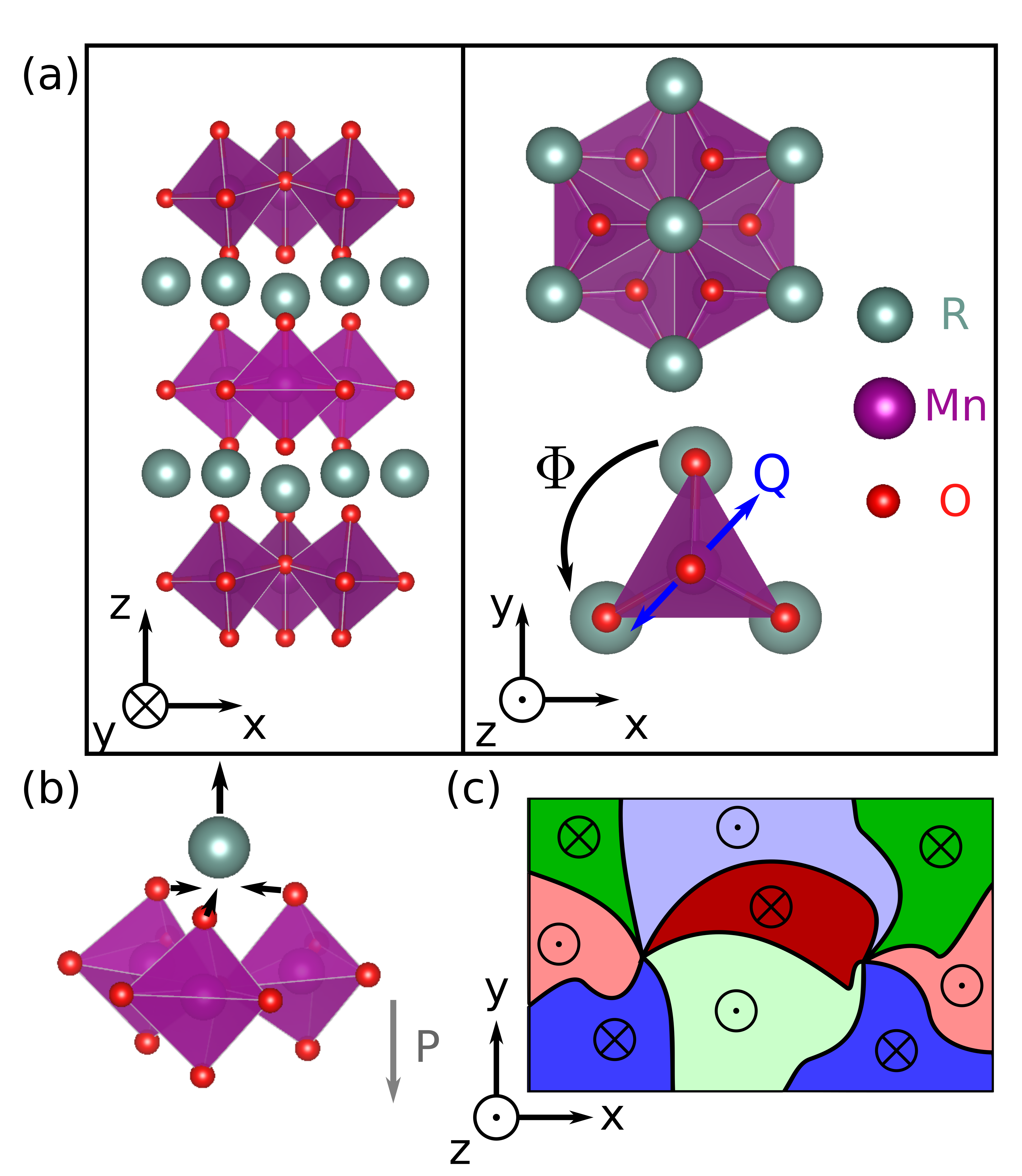
Figure 1: (a) Visualization of the structural order of hexagonal manganites. The order is given by a tilt of the MnO₅ bipyramids parametrized by the zone-boundary mode $\mathrm{K}_{3}$. The two-dimensional order parameter is illustrated in polar coordinates with $Q$ as amplitude and $\Phi$ as azimuthal angle of the MnO₅ tilt. Three neighboring bipyramids form a trimer and tilt towards a common center, which triples the unit cell [8]. (b) Visualization of the deformation of the MnO₅ bipyramids during a transition from the paraelectric to the ferroelectric phase. Small asymmetries in this process cause polarization onset [7]. (c) Schematic drawing of a conceptual distortive-ferroelectric domain structure. Topologically protected vortices are formed by the six domain states of the structural order. The circular symbols denote the improper ferroelectric out-of-plane polarization which follows an alternating pattern.

The first line in Eq. 1 corresponds to the Landau expansion of the primary structural order, and the second line corresponds to the coupling between the primary structural and the secondary ferroelectric order. The third line contains stiffness terms that result in energy penalties for domain walls (see Appendix A for more details). A schematic domain pattern resulting from the Landau expansion in Eq. 1 is visualized in Fig. 1c. There are six trimerization-polarization domain states and the associated domains form vortices of six domains in a sequence of these states and with an alternating polarization along the hexagonal axis. The vortices are topological defects because they are robust to local perturbations of the domain structure and can only be created and annihilated in pairs [5].

To model the effect of the the depolarizing field $E$ that is generated by bound charges at the surfaces and interfaces, we include an additional term in Eq. 1 [9, 10], given by

$$F_{\text{electrostatic}}=-P_{\mathrm{s}}E\;,$$ (2)

where the depolarizing electric field $E$ is obtained from the Gauss law, choosing values of $\varepsilon=0.5$ and $\varepsilon=8.9$ for the dielectric constant [11]. The model in Eq. 1 is derived for bulk crystals. Here, we adapt it to the description of thin films by using periodic boundary conditions in the in-plane directions and open boundary conditions in the out-of-plane direction, as previously done in Ref. [9].

As mentioned, we use phase-field simulations to obtain the domain structure exhibited by the hexagonal manganites [12, 13, 14, 15]. In phase-field simulations, the mesoscopic order and domain pattern of the system are described as a continuous field of order parameters. This field is initialized with random values. The subsequent evolution of the system is given by the Ginzburg-Landau equation

$$\frac{\partial\eta}{\partial t}=-\frac{\delta F}{\delta\eta},$$ (3)

where $\eta$ is an order parameter, here $Q$, $\Phi$, or $\mathcal{P}$. The expression $\delta/\delta\eta$ corresponds to a functional derivative. The electrostatic field of the system is computed from the Gauss law [10]. Finally, we compute the structure factor of the polarization-density field by taking the square of the Fourier transform of the system, in equivalence to scattering experiments. The structure factor then gives us insight on the domain-size distribution. The pair correlation of the system is computed from an inverse transform of the structure factor to derive typical domain sizes. A detailed description of the computational details and data analysis can be found in Appendix A.

III Results

Figure 2 shows domain patterns obtained by simulations with and without inclusion of the depolarizing field, both cases starting from the same initial configuration. A number of differences are immediately visible. Without consideration of electrostatic effects, our simulation results in typical domain patterns of hexagonal manganites [16, 5]. The magnitude of the polarization is constant all across the expansion of the domain outside the region of the domain walls [15, 9]. In the simulation including the electrostatic interactions in Eq. 1, however, there is a decline in polarization density that deepens the further the distance to the domain walls is. This is further illustrated in the polarization profiles Figs. 2e and 2f along the yellow cuts in Figs. 2a and 2b. This remarkable variation of the polarization distribution is a consequence of the non-local nature of the electrostatic interaction. Close to a domain wall, the electrostatic contributions from the domains on the two sides of the domain wall cancel partially, so the net electrostatic field is weak, resulting in a higher polarization magnitude. If, on the other hand, a point is far away from a domain wall, the electrostatic field is increased, resulting in the observed decline of polarization away from the walls with a dip in the approximate center of the domain. In Fig. 3, we present the distribution of the local polarization of our system. Comparing Figs. 3a and 3b, one can see that the electrostatic interaction lowers the average magnitude of the polarization of the system, but does not completely suppress it.

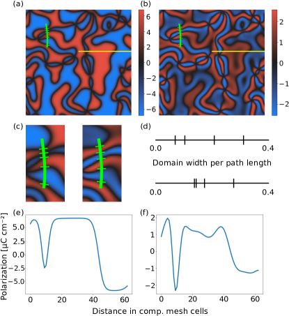
Figure 2: Dependence of improper-ferroelectric order on depolarizing field, visualized with phase-field simulations in real space. (a) Domain pattern for a simulation that ignores the electrostatic interaction. (b) Domain pattern for a simulation that includes the electrostatic interaction assuming a dielectric constant $\varepsilon=0.5$. (c) Close-up on the green paths through panels (a) (left) and (b) (right). (d) Domain size along the green path for the simulations without (top) and with (bottom) the depolarizing field. (e, f) Polarization profile along a section, shown as yellow line in (a, b). The gradient and resulting dip in polarization is clearly visible in (f).

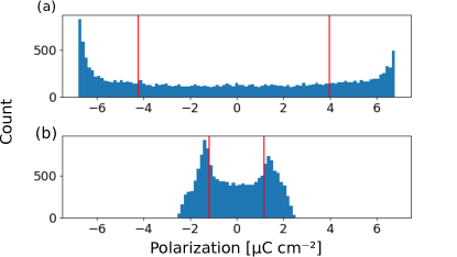
Figure 3: Histogram of the polarization per point in the computational mesh for a simulation (a) without and (b) with consideration of the depolarizing field in Eq. 1. The mean of positive/negative values are shown with red vertical bars. For both histograms, the data of Fig. 2 have been used. The average magnitude of the polarization density is lower in (b) compared to (a), which illustrates the influence of the depolarizing field.

In Fig. 4, the structure factor and the pair correlation of the polarization density of has been computed by summing the result of twenty simulations with different initial fields. This computation is equivalent to the simulation of a scattering experiment, and its technical details are described in Appendix A. Figures 4a, 4b, and 4c show the exponentially decaying structure factor and pair correlation of a system that does not include the depolarizing field. The structure factor is indicative of a broad domain-size distribution that is typical for hexagonal manganites in bulk [16] or for thin films where the depolarizing field is fully screened [17, 15]. This contrasts strikingly with the structure factor of simulations that include the electrostatic interaction. The observed ring in Fig. 4d and the pair correlation in Figs. 4e and 4f, which takes the form of a spherical wave, are indicative of a peak in the domain-size distribution, a stark difference from the case without the electrostatic interaction. The value of this peak is given by the diameter of the red disks in Fig. 4. This change in the domain patterns is further illustrated in real space in Fig. 2c, which shows an illustrative path exemplifying the change in domain size, and in and in Fig. 2d, which shows the change in domain-size distribution along this path.

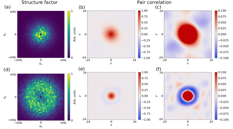
Figure 4: Structure factor and pair correlation of twenty combined simulations for (a-c) systems without depolarizing field and (d-f) systems with depolarizing field. (a) Structure factor and (b,c) pair correlation with two color scales. (d-f) Same as (a-c), but with a depolarizing field for $\varepsilon=0.5$. If the depolarizing field is present, the ring-like structure factor in (d) and the spherical wave in (e) and (f) indicate a narrow domain size distribution with a clear peak, the center of the distribution given by the diameter of the red disk in (f).

Finally, in Fig. 5 we show that the depolarizing field tends to align domain walls parallel to the z-axis. Figure 5a shows a simulation of a film that is thicker than in the previous simulations to the extent that domain walls are no longer exclusively aligned parallel to the z-direction. Instead, they start to bend towards the xy-plane, which indicates a cross-over from the thin-film regime to the bulk regime. If the electrostatic interaction is considered, as in Fig. 5b, the alignment along $z$ is drastically enhanced and most domain-wall sections lie parallel to the z-direction. On domain walls perpendicular to the z-direction, and hence perpendicular to the polarization, bound charges will accumulate at head-to-head and tail-to-tail domain walls, increasing the energy penalty for such domain walls significantly. Here the difference between excluding and including the depolarizing field in our simulations becomes particularly pronounced.

The influence of the depolarizing field on the wall alignment is further illustrated in the quantitative analysis shown in Fig. 6. We plot the fraction of domain-wall sections that are oriented perpendicular to the z-direction of systems with varying thickness for simulations with and without the electrostatic interaction (computational details in Appendix A). In films that are very thin, all domain walls are aligned along the z-direction for both scenarios because the anisotropic stiffness terms in Eq. 1 are sufficient to fully align the domain walls. As the film becomes thicker and more similar to a bulk crystal, more domain-wall sections align perpendicular to the z-direction. The ratio of perpendicular sections rises significantly more slowly for systems that include electrostatic energy contributions because of the energy penalty from charged domain walls.

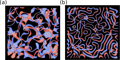
Figure 5: 3D-distribution of domain walls in simulations of thin films with and without depolarizing field. (a) Simulation ignoring electrostatic interaction and (b) simulation including electrostatic interaction. In (b), the additional electrostatic penalty for domain walls perpendicular to the z-direction cause a much stronger alignment of the domain walls along the z-axis than in (a).

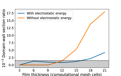
Figure 6: Fraction of domain-walls sections oriented perpendicular to the z-direction for simulations of thin films of different thickness. The depolarizing field suppresses this orientation, as shown above. An error (grey region) of about 1.5% for thin film simulations with a low number of computational mesh cells stems from numerical errors of the Poisson equation solver.

IV Discussion

In Figs. 2 to 5, we have shown that there are three are a number of effects that are caused by the depolarizing field exerted by bound charges at surfaces and interfaces of thin films. (i) The averaged magnitude of the polarization density is lowered, (ii) the polarization density declines away from the domain walls with a dip in polarization density in the approximate center of the domain, (iii) a flat domain size distribution for simulations where the depolarizing field is ignored contrasts with a distribution with a clear peak for simulations that include the depolarizing field, (iv) domain walls have a stronger tendency to align parallel to the z-axis if a depolarizing field is present.

Note that modification of domain-size is even more surprising considering that the ferroelectricity in hexagonal manganites is not only improper, but also exhibits topological defects. Despite this two-fold opposition to the action of the depolarizing field, it manifests itself with unprecedented clarity in the structure factor and cross-correlation. Our work shows that the depolarizing field can have a significant effect on the domain structure of improper ferroelectrics, even if topological defects are present, and that, in general, it is not appropriate to ignore it.

Further, the depolarizing field lowers but does not fully suppress the polarization of the system. This is characteristic for improper ferroelectrics and has been shown for a simplified Landau expansion of YMnO₃ in Sai et al. [18]. This result can be extended to Eq. 1, that is, the full Landau expansion of hexagonal manganites, and therefore our simulations also show this characteristic behavior. This contrasts with proper ferroelectrics, where a strong depolarizing field can prevent a polarization from emerging in the first place.

Finally, note that the effect of the depolarizing field depends on the dielectric constant $\varepsilon$. In our example we have chosen an artificially low value of $\varepsilon=0.5$ for the dielectric constant in order to exaggerate the effects of the depolarizing field on the domain structure. In simulations with a more realistic value of $\varepsilon=8.9$ [11], there is also a significant decline in polarization density that deepens the further the distance to the domain walls is, although the effect becomes weaker. Computing the same system as in Fig. 2f with dielectric constant $\varepsilon=8.9$, the dip is 2% of the maximum polarization density. This contrasts with the case of $\varepsilon=0.5$, where the dip is 42%.

V Conclusion

In this work, we have shown that the depolarizing field has a significant effect on the domain pattern of both the primary lattice-distortive and the secondary ferroelectric order in thin film hexagonal manganites. We find that the average magnitude polarization density of the system is lowered, the system exhibits local variations in polarization density, and there is a significant change in the domain-size distribution. Furthermore, the energy penalty of charged domain walls causes the domain walls to align parallel to the direction of the polarization.

The emergence of these effects shows that although the primary order and the topological defects are still the main driving force behind the domain structure, the effect of the depolarizing field is significant and non-negligible. We have also shown these effects are inconspicuous and only reveal themselves clearly in reciprocal space, in contrast to the domain structure of the topological defects which is apparent in real space. This may explain why these effects have not been considered in previous work.

Control of ferroelectric domains is a requirement for thin film ferroelectric devices, which is parcitularly challenging in improper ferroelectrics because the ferroelectric domain structure is pinned to the primary order. Topological defects make control even more challenging. Known avenues of control have been pinning due to local interface effects [9] and application of strain [19, 20]. Here, we have shown that the depolarizing field, despite directly acting on the secondary ferroelectric order only, also couples to the primary order and has a significant, global effect on the domain pattern of the primary order. Unlike strain, the depolarizing field preserves the isotropy in the ab-plane and does not affect the topological defects. This opens an additional avenue for control of domain patterns and the prospect of thin film devices of improper ferroelectrics.

Appendix A Detailed Numerical Methods

Terms and parameters of the Landau expansion. We use the Landau expansion as given by Artyukhin et al. [5]. The structural mode of the system is described by the terms

$$F_{\text{structural}}=\frac{a}{2}Q^{2}+{b}{4}Q^{4}+\frac{Q^{6}}{6}(c+c^{\prime}\text{cos}\,6\Phi),$$ (4)

where $Q$ and $\Phi$ are the amplitude and azimuthal angle of the structural mode respectively, and $a$, $b$, $c$, and $c^{\prime}$ are parameters of the Landau expansion. Here, we use the values $a=-2.626\,\text{eV}\text{\AA}^{-2}$, $b=3.375\,\text{eV}\text{\AA}^{-4}$, $c=0.117\,\text{eV}\text{\AA}^{-6}$, and $c^{\prime}=0.108\,\text{eV}\text{\AA}^{-3}$ [5].

The structural order couples to the ferroelectic order. This is described by the Landau terms

$$F_{\text{Ferroelectric}}=-gQ^{3}\mathcal{P}\,\text{cos}3\Phi+\frac{g^{\prime}}{2}Q^{2}P^{2},+\frac{a_{\mathcal{P}}}{2}\mathcal{P}^{2}$$ (5)

with parameters $g=1.945\,\text{eV}\,\text{\AA}^{-4}$, $g^{\prime}=9.931\,\text{eV}\text{\AA}^{-4}$, and $a_{\mathcal{P}}=0.866\,\text{ev}\,\text{\AA}^{-2}$ [5]. Because $a_{\mathcal{P}}$ is positive, the polar mode $\mathcal{P}$ cannot emerge on its own in the absence of structural order. The structural order causes the ferroelectric order, so the latter is improper.

The gradient terms of the system are given by

$$\begin{split}F_{\text{gradient}}=\frac{1}{2}\sum\limits_{i=x,y,z}\big{[}s_{Q}^{i}\big{(}\partial_{i}Q\partial_{i}Q+Q^{2}\partial_{i}\Phi\partial_{i}\Phi\big{)}&\\ +s_{\mathcal{P}}^{i}\,\partial_{i}\mathcal{P}\partial_{i}\mathcal{P}\big{]}&,\end{split}$$ (6)

with parameters $s_{\text{Q}}^{\text{z}}=15.40\,\text{eV}$, $s_{\text{Q}}^{\text{x}}=5.14\,\text{eV}$, $s_{\mathcal{P}}^{\text{z}}=50.70\,\text{eV}$, and $s_{\mathcal{P}}^{\text{z}}=8.88\text{eV}$ [5] Here, $s_{\mathcal{P}}^{\text{z}}$ has been chosen differently from [5] in order to ensure stability of the system. This is a common practice when simulating hexagonal manganites [15]. The gradient term corresponds to a penalty for non-homogeneous systems and therefore is responsible for the domain-wall energy.

Finally, a term

$$F_{\text{electrostatic}}=-PE$$ (7)

is added, where $P=\mathcal{P}\cdot 9.031\,e/365.15\,\text{\AA}^{3}$ is the polarization of the system [5] and $e$ is the elemental charge. The electric field $E$ is computed via the Gauss law. We assume that our system is a perfect insulator, and hence the total charge density is given by bound charges only according to $\rho=-\nabla P$. From the charge density, the electrostatic potential is computed via the Poisson equation $\Delta\varphi=-\rho/\varepsilon$. Finally, from the electrostatic potential, the electric field can be obtained via $E=-\nabla\varphi$.

Computational details. We obtain the Ginzburg-Landau equations by transforming Eq. (1) to Cartesian coordinates and computing its variational derivative. We choose the parameter $L=1$. We assume open boundary conditions along the hexagonal axis and periodic boundary conditions in the plane perpendicular to the hexagonal axis. In particular, we assume $E=0$ outside the thin film, which corresponds to open-electrostatic or open-circuit boundary conditions. The Ginzburg-Landau equations are then integrated in a finite difference scheme with a Runge-Kutta 4 integrator. For the main results in Figs. 2 to 4, we simulate a system of size $n_{x}\times n_{y}\times n_{z}=128\times 128\times 3$ with lattice spacing $\Delta x=\Delta y=0.1\,\text{nm}$ and $\Delta z=0.3\,\text{nm}$. We use a time step of $\Delta t=5\cdot 10^{-4}$. The dielectric constant of the material $\varepsilon$ is chosen as described in the main text. The system was iterated for $n=10^{4}$ time steps. The Poisson equation to obtain the electrostatic potential is solved using a custom V-multigrid solver using Jacobi iterations. Simulations of thick films in Fig. 5 have been performed with system of size $n_{x}\times n_{y}\times n_{z}=128\times 128\times 15$ with lattice spacing $\Delta x=\Delta y=0.2\,\text{nm}$ and $\Delta z=0.3\,\text{nm}$ and with a time step of $\Delta t=5\cdot 10^{-4}$. Simulations including the electrostatic energy were iterated for $n=10^{5}$ time steps, and a dielectric constant of $\varepsilon=0.5$ was used. The system that ignores electrostatic interactions was iterated for $n=4.3\cdot 10^{4}$ time steps to obtain domains of similar size. For the quantitative analysis of thick films in Fig. 6, simulations with system of size $n_{x}\times n_{y}=128\times 128$ with variable $n_{z}$ have been performed, with lattice spacing $\Delta x=\Delta y=0.2\,\text{nm}$ and $\Delta z=0.3\,\text{nm}$. The time step has been set to $\Delta t=5\cdot 10^{-4}$. The system was iterated for $n=10^{5}$ time steps for simulations that include and that ignore the depolarizing field. For the simulations with depolarizing field, we have set the dielectric constant to $\varepsilon=0.5$.

Data analysis. We compute the structure factor of the system by first taking a slice of the computational mesh of the thin film at $z=0$. Then, we compute the two-dimensional Fourier transform of the domain pattern and square the absolute values of the Fourier components. Fourier transformations of twenty simulations are combined to form the structure factor of the system. To compute the pair correlation, we set Fourier component at $k_{x},k_{y}=0$ to zero and then transform the structure factor back to real space.

We compute the domain-wall section ratio as in [9]. The number of domain walls $N_{\text{w}}$ is computed by counting the number of sign changes of the polar mode $\mathcal{P}(x,y,z)$ along the x-, y-, and z-axis. The ration of domain walls $\rho_{z}$ in z-direction is then computed with

$$\begin{split}\rho_{z}=\frac{1}{N_{\text{w}}}\sum\limits_{x,y=1}^{L_{x},L_{y}}\sum\limits_{z=1}^{L_{z}-1}|H(\mathcal{P}(x,y,z+1))&\\ -H(\mathcal{P}(x,y,z))&|,\end{split}$$ (8)

where $H$ is the Heaviside step function.

References

- Chanthbouala et al. [2012] A. Chanthbouala, V. Garcia, R. O. Cherifi, K. Bouzehouane, S. Fusil, X. Moya, S. Xavier, H. Yamada, C. Deranlot, N. D. Mathur, M. Bibes, A. Barthélémy, and J. Grollier, Nature Materials 11, 860 (2012), number: 10 Publisher: Nature Publishing Group.
- Trassin [2015] M. Trassin, Journal of Physics: Condensed Matter 28, 033001 (2015), publisher: IOP Publishing.
- Heron et al. [2014] J. T. Heron, J. L. Bosse, Q. He, Y. Gao, M. Trassin, L. Ye, J. D. Clarkson, C. Wang, J. Liu, S. Salahuddin, D. C. Ralph, D. G. Schlom, J. Íñiguez, B. D. Huey, and R. Ramesh, Nature 516, 370 (2014), number: 7531 Publisher: Nature Publishing Group.
- Meier and Selbach [2022] D. Meier and S. M. Selbach, Nature Reviews Materials 7, 157 (2022), number: 3 Publisher: Nature Publishing Group.
- Artyukhin et al. [2014] S. Artyukhin, K. T. Delaney, N. A. Spaldin, and M. Mostovoy, Nature Materials 13, 42 (2014), number: 1 Publisher: Nature Publishing Group.
- Fiebig et al. [2016] M. Fiebig, T. Lottermoser, D. Meier, and M. Trassin, Nature Reviews Materials 1, 1 (2016), number: 8 Publisher: Nature Publishing Group.
- Fennie and Rabe [2005] C. J. Fennie and K. M. Rabe, Physical Review B 72, 100103 (2005), publisher: American Physical Society.
- Sim et al. [2016] H. Sim, J. Oh, J. Jeong, M. D. Le, and J.-G. Park, Acta Crystallographica Section B: Structural Science, Crystal Engineering and Materials 72, 3 (2016), number: 1 Publisher: International Union of Crystallography.
- Bortis et al. [2022] A. Bortis, M. Trassin, M. Fiebig, and T. Lottermoser, Physical Review Materials 6, 064403 (2022), publisher: American Physical Society.
- Småbråten et al. [2020] D. R. Småbråten, A. Nakata, D. Meier, T. Miyazaki, and S. M. Selbach, Physical Review B 102, 144103 (2020), publisher: American Physical Society.
- Ruff et al. [2018] A. Ruff, Z. Li, A. Loidl, J. Schaab, M. Fiebig, A. Cano, Z. Yan, E. Bourret, J. Glaum, D. Meier, and S. Krohns, Applied Physics Letters 112, 182908 (2018), publisher: American Institute of Physics.
- Chen [2002] L.-Q. Chen, Annual Review of Materials Research 32, 113 (2002).
- Wang et al. [2019] J.-J. Wang, B. Wang, and L.-Q. Chen, Annual Review of Materials Research 49, 127 (2019).
- Xue et al. [2015] F. Xue, X. Wang, I. Socolenco, Y. Gu, L.-Q. Chen, and S.-W. Cheong, Scientific Reports 5, 17057 (2015), number: 1 Publisher: Nature Publishing Group.
- Xue et al. [2018] F. Xue, N. Wang, X. Wang, Y. Ji, S.-W. Cheong, and L.-Q. Chen, Physical Review B 97, 020101 (2018), publisher: American Physical Society.
- Giraldo et al. [2021] M. Giraldo, Q. N. Meier, A. Bortis, D. Nowak, N. A. Spaldin, M. Fiebig, M. C. Weber, and T. Lottermoser, Nature Communications 12, 3093 (2021), number: 1 Publisher: Nature Publishing Group.
- Meier et al. [2017] Q. Meier, M. Lilienblum, S. Griffin, K. Conder, E. Pomjakushina, Z. Yan, E. Bourret, D. Meier, F. Lichtenberg, E. Salje, N. Spaldin, M. Fiebig, and A. Cano, Physical Review X 7, 041014 (2017), publisher: American Physical Society.
- Sai et al. [2009] N. Sai, C. J. Fennie, and A. A. Demkov, Physical Review Letters 102, 107601 (2009), publisher: American Physical Society.
- Xue et al. [2017] F. Xue, X. Wang, Y. Shi, S.-W. Cheong, and L.-Q. Chen, Physical Review B 96, 104109 (2017), publisher: American Physical Society.
- Sandvik et al. [2023] O. W. Sandvik, A. M. Müller, H. W. Ånes, M. Zahn, J. He, M. Fiebig, T. Lottermoser, T. Rojac, D. Meier, and J. Schultheiß, Nano Letters , acs.nanolett.3c01638 (2023).