Universal characterization of Efimovian $D^{0}nn$ System via Faddeev Techniques

Abstract

We present a demonstration of remnant structural universality in a putative S-wave $2n$-halo-bound $D^{0}nn$ system in the $J=0,T=3/2$ channel in an idealized zero coupling limit (ZCL) scenario eliminating sub-threshold decay channels. In particular, we estimate the one- and two-body matter density form factors along with the associated mean square distances and the $n-D^{0}-n$ opening angle. For this purpose, we carry out a leading order investigation in the context of an effective quantum mechanical Faddeev approach in the momentum representation. Using Jacobi momentum representation we build a complete set of partial wave projected basis in order to reconstruct the full three-body $D^{0}nn$ wavefunctions in terms of distinct subsystem re-arrangement channels. By projecting onto the chosen basis, a set of coupled Faddeev integral equations are derived that describe the re-scattering dynamics of the coupled spin and isospin subsystems. Furthermore, by introducing short-distance two-body separable interactions, along with the scattering amplitudes (T-matrices) expressed via the so-called spectator functions, we establish a one-to-one correspondence with the well-known Skornyakov-Ter-Martirosyan integral equations used in the context of pionless/halo-EFT at leading order. A study of the regulator dependence of the integral equations reveals the underlying Efimovian character of three-body observables; in particular, those of the ground state being quite sensitive to the scale variations. Nevertheless, with the integral equations and three-body wavefunctions modified by the three-body force, such regulator dependence gets asymptotically suppressed in agreement with the renormalization group invariance. It is thereby concluded that for sufficiently small ground state three-body binding energy, the $D^{0}nn$ system in the ZCL scenario assumes a universal halo-bound structure.

I Introduction

Few-body universality broadly refers to the insensitivity of long-distance/low-energy characteristics of few-body systems to short-distance/high-energy details of interactions. They can manifest themselves in sharply contrasting manners. A common example of universality is what is manifested in the two-body sector accompanied by the occurrence of shallow two-body dimers whenever the S-wave two-body scattering length $a_{0}$ becomes positive and in fact much larger than the corresponding interaction range $r_{0}$. A renormalization group (RG) analysis of the two-body contact interactions reveals the proximity of a non-trivial infrared fixed-point that concurs with the unitary limit of the two-body interactions. However, in the pioneering works of Efimov and Danilov Efimov:1971zz ; Efimov:1970zz ; Efimov:1973awb ; Danilov:1961 , a rather exceptional universal behavior was demonstrated in the three-boson system interacting via short-distant two-body $\sim 1/r^{2}$ singular potential, with the scattering lengths fine-tuned to the unitary limit. Solving the Faddeev equations Faddeev:1961 in the hyperspherical co-ordinate representation led to the emergence of a sequence of geometrically spaced arbitrarily shallow S-wave trimers accumulating to zero energy threshold as $|a_{0}|\to\infty$. Such an emergent so-called Efimov effect Efimov:1971zz ; Efimov:1970zz ; Efimov:1973awb ; Danilov:1961 ; Braaten:2004rn ; Naidon:2016dpf , heralds the partial breakdown of the exact scale invariance of the system observables into a discrete scaling behavior. A study of the scale dependence of the three-body contact interactions shows the onset of a renormalization group (RG) limit cycle Braaten:2004rn .

Over the past two decades, Efimov universality has been extensively investigated in pionless effective field theory (${}^{\pi\!\!\!\!/}$EFT) Braaten:2004rn ; Kaplan:1996xu ; Kaplan:1998tg ; Kaplan:1998we ; Kaplan:1998sz ; vanKolck:1998bw using the momentum-space version of Faddeev scattering equations, so-called the Skornyakov-Ter-Martirosyan (STM) equations STM1 ; STM2 , in a wide variety of three-body nuclear systems. These include ordinary shallow-bound nuclear isotopes (e.g., ${}^{\,\,\,3}{\rm H}$,${}^{\,\,\,3}{\rm He}$,${}^{\,\,\,5}{\rm He}$,${}^{\,\,\,6}{\rm He}$,${}^{\,\,\,11}{\rm Li}$, ${}^{\,\,\,12}{\rm Be}$,${}^{\,\,\,14}{\rm Be}$,${}^{\,\,\,18}{\rm C}$,${}^{\,\,\,20}{\rm C}$, etc.) Bedaque:1998mb ; Bedaque:1998kg ; Bedaque:1999ve ; Bertulani:2002sz ; Bedaque:2002yg ; Canham:2008jd ; DL-Canham:2009 , exotic nuclear clusters, such as hypernuclei (e.g., ${}^{3}_{\Lambda}$H, $nn\Lambda$, ${}^{\,\,\,\,\,4}_{\Lambda\Lambda}{\rm He}$, ${}^{\,\,\,\,\,5}_{\Lambda\Lambda}{\rm H}$, ${}^{\,\,\,\,\,5}_{\Lambda\Lambda}{\rm He}$, ${}^{\,\,\,\,\,6}_{\Lambda\Lambda}{\rm He}$, $\Xi^{-}nn$, etc.) Hammer:2001ng ; Ando:2015fsa ; Hildenbrand:2019sgp ; Ando:2013kba ; Ando:2014mqa ; Ji:2014wta ; Gobel:2019jba ; Meher:2020yjr ; Meher:2020ark , as well as pure mesonic clusters including heavy charm and bottom mesons Braaten:2003he ; Raha:2017ahu ; Raha:2020sse . In addition, we refer the reader to Ref. Hammer:2019poc for a recent exhaustive review of applications of ${}^{\pi\!\!\!\!/}$EFT in the search and analyses of exotic Efimov bound states. In particular, some of these putative bound states constitute a special universal class of exotic nuclear systems termed as halo nuclei. Their quantum descriptions are defined in terms of a few physical scales independent of range and other details of short-distance pairwise interactions. Such halo systems have been extensively exploited to explore three-body universality Riisager:1994zz ; Zhukov:1993aw ; Hansen:1995pu ; Tanihata:1996 ; Jensen:2004zz . Often the neutron rich three-body hadronic clusters are identified as good halo-bound candidates owing to their typical diffuse structure and large radii with one or more loosely held “valence” neutrons orbiting about their compact cores. The core itself may either consist of a single structureless particle (as in our case), or a hadronic cluster with excitation energies much larger than the halo-neutron separation energies. This characteristic scale separation makes them amenable to a low-energy EFT description. Especially, to tackle the multi-scale S-wave threshold dynamics of halo nuclei at scales typically lower than in standard ${}^{{\pi}\!\!\!/}$EFT, an important variant, so-called the halo-EFT Bertulani:2002sz ; Bedaque:2002yg , is needed to be employed (for a recent review see Ref. Hammer:2017tjm ). Such a framework provides a starting point in exploring the possible existence and investigation of the low-energy characteristics of a putative $2n$-halo-bound $D^{0}nn$ $(J=0,T=3/2)$ system, as previously initiated in Refs. Raha:2017ahu ; Raha:2020sse .

Concurrently, meson-nucleon interactions have garnered great interest in view of their role in strangeness nuclear physics in explaining hadronic clustering phenomena. This led to the identification of a large number of exotic bound systems of mesons, nucleons, and hyperons. Especially, the study of the interaction of (anti-) kaons with nucleons or nuclei gained considerable impetus since the seminal works of Dalitz Dalitz:1959dn ; Dalitz:1959dq ; Dalitz:1960du ; Dalitz:1961dx ; Dalitz:1961dv , leading to the discovery of the well-known resonance state $\Lambda(1405)$, just below the $\bar{K}N$ threshold, thereby establishing a strongly attractive nature of $\bar{K}N$ interaction in $T=0$ isospin channel. This subsequently prompted a flurry of theoretical investigations on the possible formation of exotic kaonic nuclei using various potential model analyses Nogami:1963xqa ; Akaishi:2002bg ; Yamazaki:2007cs ; Shevchenko:2006xy ; Shevchenko:2007zz ; Ikeda:2007nz ; Ikeda:2008ub ; Dote:2008in ; Dote:2008hw ; Wycech:2008wf ; Ikeda:2010tk ; Hyodo:2011ur ; Barnea:2012qa ; Ohnishi:2017uni (also see Ref. Gal:2016boi for a recent review). However, it is well-known that dynamics of decay into other open coupled channels tend to “wash out” emergent features of three-body universality, diminishing the likelihood of Efimov state formation Braaten:2003he ; Raha:2017ahu ; Raha:2020sse ; Hyodo:2013zxa . Thus, given that the $\Lambda(1405)$ has a large decay width, $\Gamma\sim 40-70$ MeV, in comparison to its binding energy $\sim 20$ MeV, it is expected that an Efimov-like $\bar{K}NN\,(J=0,T=1/2)$ bound state is practically unfeasible. Furthermore, the ${}^{{\pi}\!\!\!/}$EFT work of Ref. Raha:2017ahu employing a sharp momentum cut-off regulator ($\Lambda_{\rm reg}$) in the Faddeev integral equations demonstrated that the particle-stable $\bar{K}NN(J=0,T=3/2)$ system remains largely unbound via Efimov attraction, with a ground state critical cut-off $\gtrsim 2$ GeV $\gg m_{\pi}$ (where $m_{\pi}$ is the pion mass), a scale too large to be amenable to a low-energy EFT description.

An analogous situation arises in the charm sector with a predominantly attractive $DN$ ($T=0$) channel leading the resonance state $\Lambda^{+}_{c}(2595)$ just below the $DN$ threshold Hofmann:2005sw ; Mizutani:2006vq and having an identical quantum number as $\Lambda(1405)$. However, unlike $\Lambda(1405)$, $\Lambda^{+}_{c}(2595)$ has a narrow width $\Gamma\sim 2.6$ MeV, making it more particle-stable. Furthermore, the potential model analysis of Ref. Bayar:2012dd posits that the $DNN\,(J=0,T=1/2)$ system is likely to form a deeply-bound trimer with binding energy $\sim 250$ MeV. However, assessing its Efimov signature has been difficult, being complicated by the presence of resonance and Coulomb effects. In contrast, the somewhat less attractive quasi-bound $DN$ ($T=1$) channel, being manifestly free of such complications may prove to be more favorable in exhibiting three-body universality signatures in the $DNN\,(J=0,T=3/2)$ channel, as hinted in Ref. Yasui:2010zz . Indeed in Ref. Raha:2017ahu , it was demonstrated that the $DN$ ($T=1$) channel manifests two-body universality upon invoking a zero-coupling limit (ZCL) idealization that excluded decay and coupled-channel effects. Furthermore, invoking the ZCL ansatz in the three-body sector, the neutron separation energy arguably becomes much smaller compared to the excitation energy of $D^{0}$-meson to the $D^{*0}(2007)$ resonance state. The distinct separation of scales thereby allows a halo-EFT Hammer:2017tjm description of the S-wave $D^{0}nn\,(J=0,T=3/2)$ system. By solving the Faddeev-like momentum-space integral equations for the three-body scattering amplitudes, the analysis in Ref. Raha:2017ahu demonstrated that an Efimov-like $D^{0}nn$ threshold ground state becomes feasible at a substantially small value of the critical cut-off, namely, $\sim 40$ MeV, in comparison to the EFT hard/breakdown scale $\lambda_{H}\sim m_{\pi}$. This indicates an encouraging prospect of an S-wave $D^{0}nn$ system manifesting as an Efimov-bound state.

In this work, we employ leading order (LO) Faddeev techniques in the momentum representation, developed in the past in Refs. Canham:2008jd ; DL-Canham:2009 ; Yamashita:2004pv ; Platter:2004he ; Platter:2004ns ; Platter:2004zs , to formulate an effective quantum mechanical methodology to assess the geometrical structure of the plausible S-wave $D^{0}nn$ bound system. Such an EFT-inspired description provides a viable means to correlate in a model-independent way the low-energy structures to the expected features of a universal halo-bound Efimov state. Such structural predictions could not only shed light on the inherent character of the hadronic clustering mechanisms but also provide valuable inputs for other ab initio calculations including lattice QCD simulations. The paper is organized as follows: In Sec. II, we begin our mathematical formulation by pedagogically presenting a brief outline of the general operator formalism of deriving the notable Faddeev equations Faddeev:1961 ; Glockle_1983 for an arbitrary three-body system. In Sec. III, we then extend the formalism to describe the dynamics of a $2n$-halo-bound $D^{0}nn$ system. For this purpose, we employ Jacobi momentum representation to build a complete set of basis states using partial wave decomposition that is needed to describe the component wavefunctions representing all possible re-arrangements of the binary subsystems. By projecting the operator form of the Faddeev equations onto the chosen basis, we derive a set of coupled integral equations describing the dynamics of the coupled spin and isospin channels for the $D^{0}nn$ system. Subsequently, we establish a one-to-one correspondence with the analogous STM integral equations derived in Ref. Raha:2017ahu using LO ${}^{{\pi}\!\!\!/}$EFT  whose solutions determine the low-energy $D^{0}nn$ observables. In Sec. IV, we demonstrate the reconstruction of the full three-body $D^{0}nn$ wavefunction in terms of different re-arrangements channels (cf. Fig. 15). We then show how the solution to component wavefunctions can be used to extract various structural features of a plausible Efimov-bound $D^{0}nn$ system, namely, the one- and two-body matter density form factors, their corresponding mean square radii, and the $n-D^{0}-n$ opening angle. In Sec. V, we report the results of our numerical evaluations in the context of the ZCL model idealization and discuss the universal physics implications. Finally, Sec. VI contains our summary and conclusions. Specific details pertaining to our adopted formalism and numerical implementation have been relegated to the appendices.

II Faddeev techniques in quantum mechanics

At non-relativistic energies, the quantum mechanics of determining the dynamics of scattering of three interacting particles ($i=1,2,3$) is obtained uniquely by numerically solving a set of three linear integral equations called the Faddeev equations. In contrast to two-body dynamics determined solely in terms of single particle motions, the three-body problem is complicated by the presence of two relative motions that are not mutually independent. This leads to the occurrence of three two-body fragmentation or re-arrangement channels ($\alpha=1,2,3$) and one break-up channel ($\alpha=0$), thereby requiring additional boundary conditions than one would expect in solving the standard three-body Schrödinger equation, or equivalently, a single Lippmann-Schwinger (LS) equation, such as

$$|\Psi^{(+)}_{\alpha}\rangle=|\phi_{\alpha}\rangle+\lim_{\varepsilon\to 0}\frac{1}{E_{\alpha}+i\varepsilon-H_{\alpha}}(V-V_{\alpha})|\Psi^{(+)}_{\alpha}\rangle\,,\quad\alpha=0,1,2,3\,.$$ (1)

Here the three-particle scattering state $|\Psi^{(+)}_{\alpha}\rangle$ in the channel $\alpha$ with complex energy $z=E_{\alpha}+i\varepsilon$ ($\varepsilon>0$) is related to the corresponding asymptotic state $|\phi_{\alpha}\rangle$ via the Möller scattering relation Taylor:2006 :

$$|\Psi^{(+)}_{\alpha}\rangle=\lim_{\varepsilon\to 0}\frac{i\varepsilon}{E_{\alpha}+i\varepsilon-H}|\phi_{\alpha}\rangle\,,\quad\alpha=0,1,2,3\,,$$ (2)

where $H_{\alpha}=H_{0}+V_{\alpha}$ is the channel Hamiltonian which is the sum of the free Hamiltonian (kinetic energy of the three-body system) $H_{0}$ and the channel potential $V_{\alpha}$, and $H=H_{0}+V$ is the full three-body Hamiltonian. The essential problem in dealing with such an LS equation is that it does not define the solution $|\Psi^{(+)}_{\alpha}\rangle$ uniquely, since the scattering state $|\Psi^{(+)}_{\beta}\rangle$, $\beta\neq\alpha$, also satisfies the corresponding homogeneous equation:

$$|\Psi^{(+)}_{\beta}\rangle=\lim_{\varepsilon\to 0}\frac{1}{E_{\beta}+i\varepsilon-H_{\alpha}}(V-V_{\alpha})|\Psi^{(+)}_{\beta}\rangle\,.$$ (3)

This criterion of non-uniqueness is the main reason for disregarding LS equations in multi-particle scattering ($n>2$). It is therefore imperative to consider an augmented version of the LS equations in a three-body problem satisfying extra boundary conditions, leading us to the Faddeev equations Faddeev:1961 . Moreover, Faddeev’s ingenious idea of decomposing the full three-body wavefunction into partitions carefully avoids the issue of disconnected contributions to the three-body scattering kernel. This becomes advantageous from the point of view of numerical evaluations. In what follows, we briefly provide a schematic framework for deriving the coupled set of integral equations in operator form for an arbitrary three-body system beginning from the three-body Schrödinger equation. In the next section, we shall present a detailed construction of the Faddeev equations for the $D^{0}nn$ system, exploiting the intrinsic symmetries of an S-wave $2n$-halo-bound system.

The Faddeev equations exploit the simplicity of breaking up a three-body system into its component (2+1)-body subsystems, namely, binary subsystems interacting with the third spectator particle. The essential idea is to introduce the partitioning of the effective three-body interaction potential into a sum of three pair-wise interaction potentials corresponding to all possible (2+1)-body re-arrangements, namely,

$$V({{\bf r_{1}},{\bf r_{2}},{\bf r_{3}}})=V_{1}(r_{23})+V_{2}(r_{31})+V_{3}(r_{12})\,,$$ (4)

where $V_{k}(r_{ij})$ is the interaction potential between the particles $i$ and $j$, with $k$ being the spectator particle. Simultaneously, one also decomposes the full three-body wavefunction $|\Psi_{\alpha}\rangle$ for a given channel $\alpha=0,1,2,3$ into three component Faddeev partition wavefunctions $|\psi_{\alpha,i}\rangle$ ($i$ being the spectator particle index), given by

$$|\Psi^{(+)}_{\alpha}\rangle=\sum^{3}_{i=1}|\psi_{\alpha,i}\rangle\,,$$ (5)

Suppressing the “$(+)$” symbol in the superscript, as well as the channel index $\alpha$, we begin by first writing the three-body Schrödinger equation for the channel in the following operator notation:

$$|\Psi\rangle=G_{0}(z)\sum_{i}V_{i}|\Psi\rangle\,,$$ (6)

where the free Green’s function or resolvent operator (representing the three-body propagator) is given by

$$G_{0}(z)\equiv({z-H_{0}})^{-1}\,,$$ (7)

where $z=E+i0_{+}$ is the total three-body energy (always assuming to have an infinitesimal positive imaginary part). Next, using Eq. (5) we express a single component wavefunction as

$$|\psi_{i}\rangle=G_{0}(z)V_{i}|\Psi\rangle=G_{0}(z)V_{i}|\psi_{i}\rangle+G_{0}(z)V_{i}\sum_{j\neq i}|\psi_{j}\rangle\,.$$ (8)

Further simplification of the above equation may be achieved by solving for the $|\psi_{i}\rangle$ component, namely,

$$|\psi_{i}\rangle=\left(1-G_{0}(z)V_{i}\right)^{-1}{G_{0}(z)V_{i}}\sum_{i\neq j}|\psi_{j}\rangle\,.$$ (9)

Since the operator in front of the summation can be iterated to all orders to obtain the two-body T-matrix for that channel (via the LS equation), namely,

$$V_{i}\left(1-G_{0}(z)V_{i}\right)^{-1} = V_{i}+V_{i}G_{0}(z)V_{i}+V_{i}G_{0}(z)V_{i}G_{0}(z)V_{i}+\cdots$$ (10)

$$= V_{i}+V_{i}G_{0}(z)t_{i}(z)\equiv t_{i}(z)\,,$$

we obtain the familiar homogeneous set of Faddeev equations given by

$$|\psi_{i}\rangle=G_{0}(z)t_{i}(z)\sum_{i\neq j}|\psi_{j}\rangle\,.$$ (11)

Furthermore, to satisfy the correct boundary conditions for a given initial channel, say, $\alpha=\alpha_{0}$, $|\psi_{\alpha_{0},i}\rangle$ must obey the inhomogeneous set of Faddeev equations expressed in the compact form:

$$|\psi_{\alpha_{0},i}\rangle=|\phi_{\alpha_{0}}\rangle\delta_{i,\alpha_{0}}+G_{0}(z)t_{i}(z)\sum_{j\neq i}|\psi_{\alpha_{0},j}\rangle\,.$$ (12)

In the following, by specializing to the case of the $D^{0}nn$ system, we derive the corresponding operator form of the Faddeev equations.

III Faddeev equations for the $D^{0}nn$ system

The LO EFT analysis presented in Refs. Raha:2017ahu ; Raha:2020sse demonstrated that the S-wave $D^{0}nn\,(J=0,T=3/2)$ system is likely to manifest Efimov states with the $DN$ ($T=1$) interactions tuned close to the unitary limit with the couplings to sub-threshold decay channels eliminated. With such a ZCL idealization, the otherwise quasi-bound $DN$ state having a small imaginary part of the complex $D^{0}n$ S-wave scattering length turns into a real-bound state having a large positive scattering length (see Ref. Raha:2017ahu for details of the extraction of the scattering lengths in the framework of a dynamical coupled-channel model). By invoking the ZCL scenario, the $D^{0}nn$ system could be pictured as a $2n$-halo nuclei with three two-body fragmentation channels: two $n+(D^{0}n)$ channels, each representing a bound $D^{0}n$ subsystem with a spectator neutron, and one $D^{0}+(nn)$ channel, representing a virtual bound $nn$ subsystem with a spectator $D^{0}$-meson. Consequently, the $D^{0}nn$ system can be described using the three Faddeev components: the first two components are represented by $|\psi_{n_{1}}\rangle$ and $|\psi_{n_{2}}\rangle$, with one of the two halo-neutrons as the spectator, while the other halo-neutron and the core $D^{0}$-meson represent the binary subsystem in each case. The third component is represented by $|\psi_{D}\rangle$, with the core $D^{0}$-meson as the spectator, while the $2n$-halo-neutrons represent the binary subsystem. However, by virtue of fermionic symmetry between identical configurations $|\psi_{n_{1}}\rangle$ and $|\psi_{n_{2}}\rangle$ upon transposition of the two neutrons, the number of independent components is reduced to two. If $\mathcal{P}$ is the permutation operator swapping the two neutrons, then we demand the anti-symmetry of the full three-body wavefunction, as well as its components, namely,

$${\mathcal{P}}|\Psi\rangle = {\mathcal{P}}\left(|\psi_{n_{1}}\rangle+|\psi_{n_{2}}\rangle+|\psi_{D}\rangle\right)$$ (13)

$$= -|\psi_{n_{2}}\rangle-|\psi_{n_{1}}\rangle-|\psi_{D}\rangle=-|\Psi\rangle\,.$$

Thus, with $|\psi_{n_{2}}\rangle$ component expressed in terms of $|\psi_{n_{1}}\rangle$, we effectively need two Faddeev partitions, namely, $|\psi_{n}\rangle$ and $|\psi_{D}\rangle$, describing all possible three-body re-arrangements, as depicted in Fig. 1. The full three-body wavefunction is then expressed as

$$|\Psi\rangle=(1-{\mathcal{P}})|\psi_{n}\rangle+|\psi_{D}\rangle\,.$$ (14)

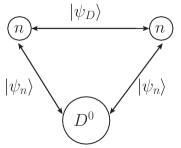
Figure 1: The Faddeev component wavefunctions for the $D^{0}nn$ system corresponding to all possible three-particle re-arrangements depending on the choice of the spectator particle.

Assuming that the $n$-$D^{0}$ and $n$-$n$ subsystems to interact via the effective potentials $V_{n}$ and $V_{D}$, respectively, the two-body T-matrices $t_{n}$ and $t_{D}$ are obtained using the standard LS equations:

$$t_{n}(z) = V_{n}+G_{0}(z)V_{n}t_{n}(z)\,,\quad\text{and}$$

$$t_{D}(z) = V_{D}+G_{0}(z)V_{D}t_{D}(z)\,.$$ (15)

Finally, noting that the permutation operator $\mathcal{P}$ leaves the T-matrices $t_{i}$ and potential $V_{i}$ invariant, the two-component coupled homogeneous Faddeev equations for the $D^{0}nn$ system can be expressed in the matrix form:

$$\begin{aligned} \begin{bmatrix}|\,\psi_{n}\rangle\,\\ \,|\psi_{D}\rangle\,\end{bmatrix}=G_{0}(z)\begin{bmatrix}-t_{n}(z){\mathcal{P}}&t_{n}(z)\\ t_{D}(z)(1-{\mathcal{P}})&0\\ \end{bmatrix}\begin{bmatrix}\,|\psi_{n}\rangle\,\\ \,|\psi_{D}\rangle\,\end{bmatrix}\end{aligned}\,.$$ (16)

For the case of negative total three-body energy, $z=E<0$, the above matrix equation has a nontrivial solution when the eigenvalue of the kernel matrix is unity. However, before attempting to solve the system of equations to obtain the three-body observables, the equations must be projected onto an appropriate complete set of basis states. This is conveniently done using the standard Jacobi representation in the momentum space.

III.1 Faddeev equations in the Jacobi representation

It is convenient to use the standard Jocobi momentum representation for the description of the three-body dynamics. In the center-of-mass frame, there are two independent momentum variables needed, namely, $\bf p$ and $\bf q$, where $\bf p$ is the relative momentum of a given two-body subsystem, and $\bf q$ is the momentum of the third spectator particle relative to the center-of-mass of the two-body subsystem. Depending upon the choice of the spectator particle three equivalent sets of Jacobi momenta are used to describe the same three-body system. Using the spectator indices $ijk$ to denote the momentum variables, the different sets of Jacobi momenta can be simply related by cyclic permutations of the indices (cf. Appendix-A).

A detailed quantum mechanical description of constructing a three-body complete partial wave Jacobi basis is provided in Appendix-A. Based on that we now define the set of Faddeev equations for the $2n$-halo $D^{0}nn$ system. The generic partial wave projected Jacobi basis constructed from plane wave states is represented as Glockle_1983

$$|pq\,\mathcal{Q}_{i}\rangle_{i} \equiv |p_{i}q_{i}\,\mathcal{Q}_{i}\rangle\,,$$ (17)

where $\mathcal{Q}_{i}$ is a collective index that specifies the spin and isospin state of the three-body system with particle $i$ as the spectator and $j$-$k$ as the binary subsystem. Thus, the different partial wave basis states for the $D^{0}nn$ system are donated as

• $|pq\,\mathcal{Q}_{D}\rangle_{D}$: $D^{0}$-meson is the spectator particle,

• $|pq\,\mathcal{Q}_{n}\rangle_{n_{1}}$: $n_{1}$-neutron is the spectator particle,

• $|pq\,\mathcal{Q}_{n}\rangle_{n_{2}}$: $n_{2}$-neutron is the spectator particle,

whereupon adopting the reasonable low-energy approximation that all the subsystem relative orbital angular momenta are in the S-wave, the spin-isospin quantum numbers of the basis are specified (see Appendix-A for details) as

$$|\mathcal{Q}_{D}\rangle_{D} \equiv \left|\big{\{}(0,0)0,(0,0)0\big{\}}00,\left(1,\frac{1}{2}\right)\frac{3}{2}\frac{3}{2}\right\rangle_{D}\,,\quad\text{and}$$

$$|\mathcal{Q}_{n}\rangle_{n} \equiv \left|\left\{\left(0,\frac{1}{2}\right)\frac{1}{2},(0,0)0\right\}00,\left(1,\frac{1}{2}\right)\frac{3}{2}\frac{3}{2}\right\rangle_{n}\,,$$ (18)

Since the two identical neutrons have opposite spins in the binary subsystem, the $|pq\,\mathcal{Q}_{D}\rangle_{D}$ basis state is anti-symmetric with respect to the two neutrons. Thus, the permutation operator $\mathcal{P}$ yields eigenvalue of -1 when operated on $|pq\,\mathcal{Q}_{D}\rangle_{D}$:

$${\mathcal{P}}|pq\,\mathcal{Q}_{D}\rangle_{D}=-|pq\,\mathcal{Q}_{D}\rangle_{D}\,.$$ (19)

As for the basis states $|pq\,\mathcal{Q}_{n}\rangle_{n_{1}}$ and $|pq\,\mathcal{Q}_{n}\rangle_{n_{2}}$, the binary subsystems are symmetric with respect to the non-identical particles. The action of $\mathcal{P}$ on these states simply interchanges the position of both neutrons with a negative sign, however, to account for the overall parity of the three-body system due to the swapping of the neutrons [cf. Eq. (13)]. Consequently, for an S-wave $D^{0}nn$ system we must have

$${\mathcal{P}}|pq\,\mathcal{Q}_{n}\rangle_{n_{1}(n_{2})}=-|pq\,\mathcal{Q}_{n}\rangle_{n_{2}(n_{1})}\,.$$ (20)

Next, we project the matrix equation, Eq. 16, onto the basis using the completeness relation, Eq. (104), given in the appendix. Notably, here we drop the summation over the set of discrete quantum numbers $\mathcal{Q}_{i}$ ($i=n,D$) since we are to consider the aforementioned specific set of such quantum numbers to describe the $D^{0}nn$ ($J=0$, $T=M_{T}=3/2$) system. Thus, we have

$${}_{n}\langle pq\,\mathcal{Q}_{n}|\psi_{n}\rangle = {}_{n}\langle pq\,\mathcal{Q}_{n}|-G_{0}(z)\,t_{n}(z)\,{\mathcal{P}}|\psi_{n}\rangle+{}_{n}\langle pq\,\mathcal{Q}_{n}|\,G_{0}(z)\,t_{n}(z)\,|\psi_{D}\rangle$$ (21)

$$= \int_{0}^{\infty}{\rm d}p^{\prime}\,p^{\prime 2}\int_{0}^{\infty}{\rm d}q^{\prime}\,q^{\prime 2}\int_{0}^{\infty}{\rm d}p^{\prime\prime}\,p^{\prime\prime 2}\int_{0}^{\infty}{\rm d}q^{\prime\prime}\,q^{\prime\prime 2}\,{}_{n}\langle pq\,\mathcal{Q}_{n}|\,G_{0}(z)\,t_{n}(z)\,|p^{\prime}q^{\prime}\,\mathcal{Q}_{n}\rangle_{n}$$

$$\qquad\times\,\Big{[}{{}_{n}\langle p^{\prime}q^{\prime}\,\mathcal{Q}_{n}|-{\mathcal{P}}|p^{\prime\prime}q^{\prime\prime}\,\mathcal{Q}_{n}\rangle_{n}}\,\,{{}_{n}\langle p^{\prime\prime}q^{\prime\prime}\,\mathcal{Q}_{n}|\psi_{n}\rangle}$$

$$\hskip 56.9055pt+\,\,{{}_{n}\langle p^{\prime}q^{\prime}\,\mathcal{Q}_{n}|p^{\prime\prime}q^{\prime\prime}\,\mathcal{Q}_{D}\rangle_{D}}\,\,{{}_{D}\langle p^{\prime\prime}q^{\prime\prime}\,\mathcal{Q}_{D}|\psi_{D}\rangle}\Big{]}\,,\qquad\text{and}$$

$${}_{D}\langle pq\,\mathcal{Q}_{D}|\psi_{D}\rangle = {}_{D}\langle pq\,\mathcal{Q}_{D}|\,G_{0}(z)\,t_{D}(z)(1-{\mathcal{P}})\,|\psi_{n}\rangle$$ (22)

$$= \int_{0}^{\infty}{\rm d}p^{\prime}\,p^{\prime 2}\int_{0}^{\infty}{\rm d}q^{\prime}\,q^{\prime 2}\int_{0}^{\infty}dp^{\prime\prime}\,p^{\prime\prime 2}\int_{0}^{\infty}dq^{\prime\prime}\,q^{\prime\prime 2}\,{}_{D}\langle pq\,\mathcal{Q}_{D}|\,G_{0}(z)\,t_{D}(z)\,|p^{\prime}q^{\prime}\mathcal{Q}_{D}\rangle_{D}$$

$$\qquad\times\,{{}_{D}\langle p^{\prime}q^{\prime}\,\mathcal{Q}_{D}|(1-{\mathcal{P}})|p^{\prime\prime}q^{\prime\prime}\,\mathcal{Q}_{n}\rangle_{n}}\,\,{{}_{n}\langle p^{\prime\prime}q^{\prime\prime}\,\mathcal{Q}_{n}|\psi_{n}\rangle}\,,$$

where it is understood that the integration variables are all expressed in terms of a specific choice of the spectator representation, although the final results are independent of any specific choice. For concreteness, let us choose to express the intermediate states in terms of the Jacobi momenta where a neutron is the spectator, namely, $p^{\prime}\equiv p^{\prime}_{n},\,p^{\prime\prime}\equiv p^{\prime\prime}_{n},\,q^{\prime}\equiv q^{\prime}_{n},\,q^{\prime\prime}\equiv q^{\prime\prime}_{n}$. Thus,

$${}_{n}\langle p^{\prime}q^{\prime}\,\mathcal{Q}_{n}|p^{\prime\prime}q^{\prime\prime}\,\mathcal{Q}_{D}\rangle_{D} \equiv {}_{n}\langle p^{\prime}_{n}q^{\prime}_{n}\,\mathcal{Q}_{n}|p^{\prime\prime}_{n}q^{\prime\prime}_{n}\,\mathcal{Q}_{D}\rangle_{D}\,,\quad\text{and}$$

$${}_{D}\langle p^{\prime}q^{\prime}\,\mathcal{Q}_{D}|p^{\prime\prime}q^{\prime\prime}\,\mathcal{Q}_{n}\rangle_{n} \equiv {}_{D}\langle p^{\prime}_{n}q^{\prime}_{n}\,\mathcal{Q}_{D}|p^{\prime\prime}_{n}q^{\prime\prime}_{n}\,\mathcal{Q}_{n}\rangle_{n}\,.$$

We further notice that the coupled integral equations comprise several two-body LS kernel-matrix elements of the form ${}_{i}\langle pq\,\mathcal{Q}_{i}|\,G_{0}(z)t_{i}(z)\,|p^{\prime}q^{\prime}\,\mathcal{Q}_{i}\rangle_{i}$ and overlap matrix elements of the form ${}_{i}\langle p^{\prime}q^{\prime}\,\mathcal{Q}_{i}|p^{\prime\prime}q^{\prime\prime}\,\mathcal{Q}_{j}\rangle_{j}$. Their expressions are analytically derived in the ensuing treatment using an effective quantum mechanical approach where only LO effective separable potentials are used. Our methodology is an essential adoption of the universality-based effective potential technique developed in Refs. Platter:2004he ; Platter:2004ns ; Platter:2004zs for resonant systems of three and four bosons, and subsequently extended to the study of $2n$-halo nuclei, such as the ⁶He, ²⁰C, etc. Canham:2008jd ; DL-Canham:2009 ; Ji:2014wta ; Gobel:2019jba .

III.2 Two-body kernel matrix elements ${}_{i}\langle pq\,\mathcal{Q}_{i}|G_{0}t_{i}|p^{\prime}q^{\prime}\,\mathcal{Q}_{i}\rangle_{i}$

In Appendix-B, we presented a derivation of the general form of the two-body T-matrix [cf. Eq. 130] starting from an S-wave non-local separable potential in momentum representation with a LO contact interactions $C_{0}$ of the form

$$\langle{\mathbf{p}}|V_{\rm eff}|{\mathbf{p}}^{\prime}\rangle\,\stackrel{{\scriptstyle\rm S-wave}}{{\longrightarrow}}\,\chi(p)\,C_{0}\,\chi(p^{\prime})\,.$$ (23)

Here, $\bf p$/$\bf p^{\prime}$ is the two-body incoming/outgoing relative momentum, and the $\chi(p)$s are functions, so-called form factors, related to the factorized residues at the poles of the corresponding T-matrix or propagator. The formalism is pertinent to the treatment of halo systems where the binary subsystems are also likely to exhibit universality with distinct separation of scales. Moreover, owing to the separable nature of the T-matrix, the LS equation is analytically solvable allowing us to directly fix the coupling constant $C_{0}$ from the two-body bound/anti-bound state pole of a given subsystem, as demonstrated in Appendix-B. In the absence of sub-threshold decay channels, the form factors are real and may be used as regulators to suppress high-momentum modes beyond a certain hard/cut-off scale, i.e., for $p,p^{\prime}\geq\Lambda_{H}$, where the effective potential breaks down. In this way, one can directly relate to a low-energy EFT description with zero-range contact interactions. In particular, for the purpose of numerical evaluations, it is customary to introduce a sharp momentum finite cut-off $\Lambda_{\rm reg}$ as the ultraviolet (UV) limit of the Faddeev integral equations which is easily implemented via a simple Heaviside step function, $\chi(p)=\Theta(\Lambda_{\rm reg}-p)$, for the S-wave form factors in the kernel with the integration UV limits taken to infinity. However, it must be mentioned that the low-energy observables are expected to be regulator-independent as $\Lambda_{\rm reg}\to\infty$, consistent with RG invariance of the theory. Since we wish to relate the results of the effective potential approach to those obtained in Ref. Raha:2017ahu using pionless EFT, a natural choice of the UV regulator cut-off is $\Lambda_{\rm reg}\gtrsim\Lambda_{H}\sim m_{\pi}$.

The kernel matrix elements associated with the Faddeev equations, Eqs. (21) and (22), correspond to a putative bound $D^{0}nn$ system with three-body binding energy, Re$(z)=E=-B_{3}<0$ and represented as:

$${}_{i}\langle pq\,\mathcal{Q}_{i}|\,G_{0}(z)t_{i}(z)\,|p^{\prime}q^{\prime}\,\mathcal{Q}_{i}\rangle_{i}=-\mathcal{G}_{0}^{(i)}(p,q;B_{3})\,\,{}_{i}\langle pq\,\mathcal{Q}_{i}|\,t_{i}(z)\,|p^{\prime}q^{\prime}\,\mathcal{Q}_{i}\rangle_{i}\,,$$

where the three-particle free Green’s functions are proportional to

$$\mathcal{G}_{0}^{(n)}(p,q;B_{3}) = \bigg{[}B_{3}+\frac{p^{2}}{2\mu_{nD}}+\frac{q^{2}}{2\mu_{n(nD)}}\bigg{]}^{-1}=\bigg{[}B_{3}+\frac{y+1}{2yM_{n}}p^{2}+\frac{y+2}{2(y+1)M_{n}}q^{2}\bigg{]}^{-1}\,,\quad\text{and}$$

$$\mathcal{G}_{0}^{(D)}(p,q;B_{3}) = \bigg{[}B_{3}+\frac{p^{2}}{M_{n}}+\frac{q^{2}}{2\mu_{D(nn)}}\bigg{]}^{-1}=\bigg{[}B_{3}+\frac{p^{2}}{M_{n}}+\frac{y+2}{4yM_{n}}q^{2}\bigg{]}^{-1}\,,$$ (24)

depending on the choice of the spectator particle $i=n,D$, with $M_{n}$ being the neutron mass, and $M_{D}=yM_{n}$ being the $D^{0}$-meson mass. The reduced masses $\mu_{nD}$, $\mu_{n(nD)}$ and $\mu_{D(nn)}$ are defined in Appendix A. While the former Green’s function corresponds to the exchange of the $D^{0}$-meson between the two neutrons, the latter corresponds to the exchange of a neutron between the other neutron and the $D^{0}$-meson. The T-matrix $t_{i}(z)$ being an embedding in the subspace of the binary subsystem $i$, it must be diagonal with respect to the spectator particle quantum numbers, and thereby evaluated at the shifted energy, $z_{i}=z-\frac{q^{\prime 2}_{i}}{2\mu_{i(jk)}}$, namely,

$${}_{i}\langle pq\,\mathcal{Q}_{i}|\,t_{i}(z_{i})\,|p^{\prime}q^{\prime}\,\mathcal{Q}_{i}\rangle_{i} = \delta_{JJ^{\prime}}\,\delta_{M_{J}M_{J}^{\prime}}\,\delta_{LL^{\prime}}\,\delta_{SS^{\prime}}\,\delta_{TT^{\prime}}\,\delta_{M_{T}M_{T}^{\prime}}\,\delta_{\mathcal{J}\,\mathcal{J}^{\prime}}\,\delta_{\lambda\lambda^{\prime}}\,\delta_{\sigma\sigma^{\prime}}\,\delta_{\tau\tau^{\prime}}$$ (25)

$$\,\,\,\times\,\frac{\delta(q-q^{\prime})}{qq^{\prime}}\,\,{}_{i}\langle p(l,s)\mathcal{j}t|\,\widehat{t}_{i}(z_{i})\,|p^{\prime}(l^{\prime},s^{\prime})\mathcal{j}^{\prime}t^{\prime}\rangle_{i}\,.$$

Now it is straightforward to show that the partial wave projected T-matrix ${}_{i}\langle p(l,s)\mathcal{j}t|\,\widehat{t}_{i}(z_{i})\,|p^{\prime}(l^{\prime},s^{\prime})\mathcal{j}^{\prime}t^{\prime}\rangle_{i}$ is related to LO S-wave scattering amplitude $T_{i}(p,p^{\prime};z_{i})$ by the simple relation:

$${}_{i}\langle p(0,s)\mathcal{j}t|\,\widehat{t}_{i}(z_{i})\,|p^{\prime}(0,s^{\prime})\mathcal{j}^{\prime}t^{\prime}\rangle_{i}={}_{i}\langle p|\,\widehat{t}_{i}(z_{i})\,|p^{\prime}\rangle_{i}\,\delta_{ss^{\prime}}\delta_{\mathcal{j}\mathcal{j}^{\prime}}\delta_{tt^{\prime}}=4\pi\,T_{i}(p,p^{\prime};z_{i})\,\delta_{ss^{\prime}}\delta_{\mathcal{j}\mathcal{j}^{\prime}}\delta_{tt^{\prime}}\,,$$ (26)

where it is assumed that the interactions in the binary subsystems conserve their total spin $\mathcal{j}$, intrinsic spin $s$, and isospin $t$, with the obvious exception of Coulomb interactions which are excluded in our formalism.

As we wish to explore the plausibility of a halo-bound $D^{0}nn$ system where the binary subsystems are also bound/anti-bound, it is of interest to evaluate the T-matrices at the two-body energies, $z_{i}=\mathscr{E}_{i}+i0_{+}$, expressed in terms of the three-body bound state energy $B_{3}$. Thus, for the binary subsystems, we define the following momentum functions:

$$\gamma_{n}(q;B_{3}) \equiv \sqrt{-2\mu_{nD}\mathscr{E}_{n}(q)}=\sqrt{\frac{y}{y+1}\bigg{(}2M_{n}B_{3}+\frac{y+2}{y+1}q^{2}\bigg{)}}\,,\quad\text{and}$$

$$\gamma_{D}(q;B_{3}) \equiv -\sqrt{-2\mu_{nn}\mathscr{E}_{D}(q)}=-\sqrt{M_{n}B_{3}+\frac{y+2}{4y}q^{2}}\,.$$ (27)

We then explicitly obtain the following forms for the kernel matrix elements after S-wave projection:

$${}_{i}\langle pq(\mathcal{j},\mathcal{J})JM_{J},TM_{T}|\,G_{0}(z)t_{i}(z)\,|p^{\prime}q^{\prime}(\mathcal{j},\mathcal{J})JM_{J},TM_{T}\rangle_{i} = -4\pi\mathcal{G}_{0}^{(i)}(p,q;B_{3})\frac{\delta(q-q^{\prime})}{qq^{\prime}}$$ (28)

$$\qquad\times\,T_{i}(p,p^{\prime};z_{i})\,,$$

where $\mathcal{G}^{(i)}_{0}$’s are defined in Eq. (24), and the LO S-wave two-body T-matrices are expressed in the separable form (see Appendix-B):

$$T_{i}(p,p^{\prime};\mathscr{E}_{i})=-\frac{1}{4\pi}\chi(p)\,\chi(p^{\prime})\,\tau_{i}(q^{\prime};B_{3})\,,$$ (29)

with the terms containing information on the short-range LO S-wave effective interactions, given by

$$\tau_{n}(q;B_{3}) = \frac{y+1}{\pi yM_{n}}\bigg{[}-\frac{1}{a_{nD}}\,\frac{2}{\pi}\arctan\big{(}|a_{nD}|{\Lambda_{\rm reg}}\big{)}+\gamma_{n}(q;B_{3})\,\frac{2}{\pi}\arctan\bigg{(}\frac{\Lambda_{\rm reg}}{\gamma_{n}(q;B_{3})}\bigg{)}\bigg{]}^{-1}\,,\,\text{and}$$

$$\tau_{D}(q;B_{3}) = \frac{2}{\pi M_{n}}\bigg{[}-\frac{1}{a_{nn}}\,\frac{2}{\pi}\arctan\big{(}|a_{nn}|{\Lambda_{\rm reg}}\big{)}+\gamma_{D}(q;B_{3})\,\frac{2}{\pi}\arctan\bigg{(}\frac{\Lambda_{\rm reg}}{\gamma_{D}(q;B_{3})}\bigg{)}\bigg{]}^{-1}\,,$$ (30)

where $a_{nn}$ and $a_{nD}$ are the S-wave $n$-$n$ and $n$-$D$ scattering lengths, respectively. Notice that when $q=0$ the two-body bound (anti-bound) states correspond to the respective poles in the above T-matrices which at LO correspond to binding (virtual) momenta, namely,

$$\text{{\it real} bound:}\quad\gamma_{n}(q=0;B_{3}=B_{nD}) = \sqrt{2\mu_{nD}B_{nD}}=\frac{1}{a_{nD}}>0\,,\quad\text{and}$$

$$\text{{\it virtual} bound:}\quad\gamma_{D}(q=0;B_{3}=B_{nn}) = -\sqrt{2\mu_{nn}B_{nn}}=\frac{1}{a_{nn}}<0\,,$$ (31)

with the three-body binding energy $B_{3}$ coinciding with the two-body binding energy, $B_{2}=B_{nn}$ and $B_{2}=B_{nD}$, respectively. We note here that analogous expressions for the T-matrices were obtained previously in Refs. Canham:2008jd ; DL-Canham:2009 ; Platter:2004he ; Platter:2004ns ; Platter:2004zs in the context of universality-based studies of bosonic systems, and in the investigation of ²⁰C as a $2n$-halo nucleus.

III.3 Overlap matrix elements ${}_{i}\langle pq\,\mathcal{Q}_{i}|p^{\prime}q^{\prime}\,\mathcal{Q}_{j}\rangle_{j}$

Next, we discuss the evaluation of the overlap matrix elements of the form ${}_{i}\langle pq\,\mathcal{Q}_{i}|p^{\prime}q^{\prime}\,\mathcal{Q}_{j}\rangle_{j}$ ($i,j=n,D$) of the Faddeev equations, Eqs. (21) and (22), which yield the transition amplitudes between different three-body subsystem re-arrangements. These are obtained via evaluation of the re-coupling coefficient between different Jacobi momentum representations. For details of the general method of derivation, we refer the reader to Ref. Glockle_1983 . Here we simply quote the end results for the S-wave projected overlap matrix elements relevant to the $D^{0}nn$ system. The generic result is given by

$${}_{i}\langle pq\,\mathcal{Q}_{i}|p^{\prime}q^{\prime}\,\mathcal{Q}_{j}\rangle_{j}\equiv{}_{i}\langle p_{i}q_{i}\,\mathcal{Q}_{i}|p^{\prime}_{i}q^{\prime}_{i}\,\mathcal{Q}_{j}\rangle_{j}=\int_{-1}^{1}{\rm d}x\,\frac{\delta(p-\pi_{ij})}{p\pi_{ij}}\frac{\delta(p^{\prime}-\pi^{\prime}_{ij})}{p^{\prime}\pi^{\prime}_{ij}}\,\mathscr{G}^{(ij)}\,,$$ (32)

where $x\equiv\hat{\bf q}_{i}\cdot\hat{\bf q}^{\prime}_{i}$ is the cosine of the angle between the initial and final spectator relative momenta with respect to the binary subsystem $j$-$k$, such that

$$\pi_{ij}(q,q^{\prime};x) = \sqrt{\left(\frac{\mu_{jk}}{m_{k}}\right)^{2}q^{2}+q^{\prime 2}+2\left(\frac{\mu_{jk}}{m_{k}}\right)qq^{\prime}x}\,,\quad\text{and}$$

$$\pi^{\prime}_{ij}(q,q^{\prime};x) = \sqrt{q^{2}+\left(\frac{\mu_{ki}}{m_{k}}\right)^{2}q^{\prime 2}+2\left(\frac{\mu_{ki}}{m_{k}}\right)qq^{\prime}x}\,\,,$$ (33)

are the magnitudes of the shifted momenta. The quantity

$$\mathscr{G}^{(ij)}=\mathscr{G}^{(ji)}\equiv{}_{i}\langle\mathcal{Q}_{i}|\mathcal{Q}_{j}\rangle_{j} = \frac{1}{2}\sqrt{\hat{s}\,\hat{\mathcal{j}}\,\hat{t}\,\hat{\mathcal{J}}\,\hat{s^{\prime}}\,\hat{\mathcal{j}^{\prime}}\,\hat{t^{\prime}}\,\hat{\mathcal{J}^{\prime}}}\,(-1)^{t_{i}+t_{j}+t_{k}+T}\,(-1)^{s_{i}+s_{j}+s_{k}+S}$$ (34)

$$\!\!\!\times\,\begin{Bmatrix}t_{j}&t_{k}&t\\ t_{i}&T&t^{\prime}\\ \end{Bmatrix}\begin{Bmatrix}s_{j}&s_{k}&s\\ s_{i}&S&s^{\prime}\\ \end{Bmatrix}\sum_{S}\hat{S}\begin{Bmatrix}0&s&\mathcal{j}\\ 0&\sigma&\mathcal{J}\\ 0&S&J\\ \end{Bmatrix}\begin{Bmatrix}0&s^{\prime}&\mathcal{j}^{\prime}\\ 0&\sigma^{\prime}&\mathcal{J}^{\prime}\\ 0&S&J\\ \end{Bmatrix}\,,$$

is a simple geometrical constant arising due to the re-coupling of the Jacobi state angular momenta and isospins between two different spectator representations with indices $i$ and $j$. Each overlap matrix has four momenta, of which any two of them could be eliminated in favor of the other two upon integration over the two delta functions in Eq. (32). Here, we prefer to eliminate $p$ and $p^{\prime}$ in favor of $q$ and $q^{\prime}$. The following three cases of the overlap matrix elements relevant to the $D^{0}nn$ system are in order:

• Case I: Due to swapping of the two spectator neutrons:

  $${}_{n_{1}}\langle pq\,{\mathcal{Q}}_{n}|\,\mathcal{P}|p^{\prime}q^{\prime}\,{\mathcal{Q}}_{n}\rangle_{n_{1}}=-\,{}_{n_{1}}\!\langle pq\,{\mathcal{Q}}_{n}|p^{\prime}q^{\prime}\,{\mathcal{Q}}_{n}\rangle_{n_{2}}\,.$$ (35)

  In this case, since the states $|pq\,{\mathcal{Q}}_{n}\rangle_{n_{1}}$ and $|p^{\prime}q^{\prime}\,{\mathcal{Q}}_{n}\rangle_{n_{2}}$ correspond to identical binary subsystem $n$-$D^{0}$, the particle re-arrangement leads to the same set of discrete quantum numbers, i.e., $\mathcal{Q}_{n_{1}}=\mathcal{Q}_{n_{2}}\equiv\mathcal{Q}_{n}$, as displayed in Table. 1. In particular, the Pauli principle demands that the halo-neutrons must have opposite intrinsic spins for an S-wave three-body system. Consequently, the total spin of the system should be the same as the spin of the core $D^{0}$-meson which is obviously 0.

  $nD^{0}$-subsystem	$l=0$	$s=1/2$	${\bf\mathcal{j}}=1/2$	$t=1$
  $n$-spectator	$\lambda=0$	$\sigma=1/2$	${\bf\mathcal{J}}=1/2$	$\tau=1/2$
  Three-body	$L=0$	$S=0$	$J=0$	$T=3/2$

  Table 1: Various spin-isospin quantum numbers corresponding to the state $|\mathcal{Q}_{n}\rangle_{n}$.

  By using these quantum numbers in Eq. (34) the value of the geometrical re-coupling constant is obtained as $\mathscr{G}^{(nn)}\equiv{}_{n_{1}}\langle\mathcal{Q}_{n}|\mathcal{Q}_{n}\rangle_{n_{2}}=1/2$, which leads to the result:

  $${}_{n_{1}}\langle pq\,\mathcal{Q}_{n}|p^{\prime}q^{\prime}\,\mathcal{Q}_{n}\rangle_{n_{2}}\equiv{}_{n_{1}}\langle p_{n_{1}}q_{n_{1}}\,\mathcal{Q}_{n}|p^{\prime}_{n_{1}}q^{\prime}_{n_{1}}\,\mathcal{Q}_{n}\rangle_{n_{2}}=\frac{1}{2}\int_{-1}^{1}{\rm d}x\frac{\delta(p-\pi_{nn})}{p\pi_{nn}}\frac{(p^{\prime}-\pi^{\prime}_{nn})}{p^{\prime}\pi^{\prime}_{nn}}\,,$$ (36)

  with the “shifted” momenta given as

  $$\pi_{nn}(q,q^{\prime};x) = \sqrt{\left(\frac{1}{y+1}\right)^{2}q^{2}+q^{\prime 2}+2\left(\frac{1}{y+1}\right)qq^{\prime}x}\,,\quad\text{and}$$

  $$\pi^{\prime}_{nn}(q,q^{\prime};x) \equiv \pi_{nn}(q^{\prime},q;x)=\sqrt{q^{2}+\left(\frac{1}{y+1}\right)^{2}q^{\prime 2}+2\left(\frac{1}{y+1}\right)qq^{\prime}x}\,\,.$$ (37)

• Case II: Due to interchange of a spectator neutron with the core $D^{0}$-meson as a spectator:

  $${}_{n}\langle pq\,\mathcal{Q}_{n}|p^{\prime}q^{\prime}\,\mathcal{Q}_{D}\rangle_{D}\,.$$

  In this case, since the state $|pq\,\mathcal{Q}_{n}\rangle_{n}$ corresponds to the $n$-$D^{0}$ binary subsystem, the unprimed quantum numbers are identical to those in Table 1. Whereas, the state $|p^{\prime}q^{\prime}\,\mathcal{Q}_{D}\rangle_{D}$ corresponds to the $n$-$n$ binary subsystem with the core $D^{0}$-meson as the spectator. The set of discrete quantum numbers associated with the latter is displayed in Table 2.

  $nn$-subsystem	$l^{\prime}=0$	$s^{\prime}=0$	${\bf\mathcal{j}^{\prime}}=0$	$t^{\prime}=1$
  $D^{0}$-spectator	$\lambda^{\prime}=0$	$\sigma^{\prime}=0$	${\bf\mathcal{J}^{\prime}}=0$	$\tau^{\prime}=1/2$
  Three-body	$L=0$	$S=0$	$J=0$	$T=3/2$

  Table 2: Various spin-isospin quantum numbers corresponding to the state $|\mathcal{Q}_{D}\rangle_{D}$.

  By using in Eq. (34) the unprimed and primed set of quantum numbers from Tables 1 and 2, respectively, we obtain the value of the re-coupling constant as $\mathscr{G}^{(nD)}_{\mathcal{Q}_{n}\mathcal{Q}_{D}}\equiv{}_{n}\langle\mathcal{Q}_{n}|\mathcal{Q}_{n}\rangle_{D}=1/2$, leading to the result:

  $${}_{n}\langle p_{n}q_{n}\,\mathcal{Q}_{n}|p^{\prime}_{n}q^{\prime}_{n}\,\mathcal{Q}_{D}\rangle_{D}\equiv{}_{n}\langle pq\,\mathcal{Q}_{n}|p^{\prime}q^{\prime}\,\mathcal{Q}_{D}\rangle_{D}=\frac{1}{2}\int^{1}_{-1}{\rm d}x\frac{\delta(p-\pi_{nD})}{p\pi_{nD}}\frac{\delta(p^{\prime}-\pi^{\prime}_{nD})}{p^{\prime}\pi^{\prime}_{nD}}\,,$$ (38)

  with the shifted momenta given as

  $$\pi_{nD}(q,q^{\prime};x)=\sqrt{\left(\frac{y}{y+1}\right)^{2}q^{2}+q^{\prime 2}+2\left(\frac{y}{y+1}\right)qq^{\prime}x}\,,\qquad\text{and}$$

  $$\pi^{\prime}_{nD}(q,q^{\prime};x)=\sqrt{q^{2}+\frac{q^{\prime 2}}{4}+qq^{\prime}x}\,.$$ (39)

• Case III: Due to the interchange of the spectator core $D^{0}$-meson with any one of the halo-neutrons as the spectator:

  $${}_{D}\langle pq\,\mathcal{Q}_{D}|p^{\prime}q^{\prime}\,\mathcal{Q}_{n}\rangle_{n}\,.$$

  In this case with the primed and unprimed sets of discrete quantum numbers swapped with respect to Case II, leave the re-coupling constant unchanged, namely, $\mathscr{G}^{(Dn)}\equiv{}_{D}\langle\mathcal{Q}_{n}|\mathcal{Q}_{n}\rangle_{n}=1/2$. The corresponding result is

  $${}_{D}\langle p_{n}q_{n}\,\mathcal{Q}_{D}|p^{\prime}_{n}q^{\prime}_{n}\,\mathcal{Q}_{n}\rangle_{n}\equiv{}_{D}\langle pq\,\mathcal{Q}_{D}|p^{\prime}q^{\prime}\,\mathcal{Q}_{n}\rangle_{n} = \frac{1}{2}\int^{1}_{-1}{\rm d}x\frac{\delta(p-\pi_{Dn})}{p\pi_{Dn}}\frac{\delta(p^{\prime}-\pi^{\prime}_{Dn})}{p^{\prime}\pi^{\prime}_{Dn}}$$ (40)

  $$= \frac{1}{2}\int^{1}_{-1}{\rm d}x\frac{\delta(p-\pi^{\prime}_{nD})}{p\pi^{\prime}_{nD}}\frac{\delta(p^{\prime}-\pi_{nD})}{p^{\prime}\pi_{nD}}\,,\quad\,$$

  with the shifted momenta given as

  $$\pi_{Dn}(q,q^{\prime};x) \equiv \pi^{\prime}_{nD}(q^{\prime},q;x)=\sqrt{\frac{q^{2}}{4}+q^{\prime 2}+qq^{\prime}x}\,,\quad\text{and}$$

  $$\pi^{\prime}_{Dn}(q,q^{\prime};x) \equiv \pi_{nD}(q^{\prime},q;x)=\sqrt{q^{2}+\left(\frac{y}{y+1}\right)^{2}q^{\prime 2}+2\left(\frac{y}{y+1}\right)qq^{\prime}x}\,.$$ (41)

III.4 Faddeev equations for the S-wave $2n$-halo $D^{0}nn$ system at LO

Having all the necessary ingredients, namely, the various LO kernel and overlap matrix elements, we can now spell out the explicit form of the Faddeev equations for the $2n$-halo $D^{0}nn$ system at LO. Using the results of Eqs. (28), (29), (30), (36), (37), (38), (39), (40) and (41) in Eqs. (21) and (22), and then integrating over the delta functions, we obtain the following set of homogeneous integral equations Canham:2008jd ; DL-Canham:2009 ; Platter:2004he ; Platter:2004ns ; Platter:2004zs :

$$\psi_{n}(p,q) = \frac{1}{2}\mathcal{G}^{(n)}_{0}(p,q;B_{3})\,\chi(p)\,\tau_{n}(q;B_{3})\int_{0}^{\infty}{\rm d}{q^{\prime\prime}}q^{\prime\prime 2}\int_{-1}^{1}{\rm d}x$$

$$\times\,\bigg{[}\chi\left(\pi_{nn}(q,q^{\prime\prime};x)\right)\psi_{n}\left(\pi_{nn}(q^{\prime\prime},q;x),q^{\prime\prime}\right)+\chi\left(\pi_{nD}(q,q^{\prime\prime};x)\right)\psi_{D}\left(\pi^{\prime}_{nD}(q,q^{\prime\prime};x),q^{\prime\prime}\right)\bigg{]},$$

and

$$\psi_{D}(p,q) = \mathcal{G}^{(D)}_{0}(p,q;B_{3})\,\chi(p)\,\tau_{D}(q;B_{3})$$ (43)

$$\qquad\times\,\int_{0}^{\infty}{\rm d}{q^{\prime\prime}}q^{\prime\prime 2}\int_{-1}^{1}{\rm d}x\,\chi\left(\pi^{\prime}_{nD}(q^{\prime\prime},q;x)\right)\psi_{n}\left(\pi_{nD}(q^{\prime\prime},q;x),q^{\prime\prime}\right),$$

where we define the component wavefunctions as $\psi_{i}(p,q)\equiv{}_{i}\langle pq\,\mathcal{Q}_{i}|\psi_{i}\rangle$.

For the sake of simplicity of numerical solutions, it is advantageous to introduce the so-called spectator functions $F_{i}(q)$ Mitra:1969 defining each of the distinct Faddeev components, namely,

$$\psi_{i}(p,q)=\mathcal{G}^{(i)}_{0}(p,q;B_{3})\,\chi(p)\,\tau_{i}(q;B_{3})\,F_{i}(q)\,;\quad i=n,D\,.$$ (44)

Thus, we end up with the following set of single-variable coupled integral equations which is easier to solve numerically Canham:2008jd ; DL-Canham:2009 ; Platter:2004he ; Platter:2004ns ; Platter:2004zs :

$$F_{n}(q) = \frac{1}{2}\int_{0}^{\infty}{\rm d}{q^{\prime}}q^{\prime 2}\int_{-1}^{1}{\rm d}x\Big{[}\chi\left(\pi_{nn}(q,q^{\prime};x)\right)\,\chi\left(\pi_{nn}(q^{\prime},q;x)\right)$$

$$\hskip 142.26378pt\times\,\mathcal{G}^{(n)}_{0}(\pi_{nn}(q^{\prime},q;x),q^{\prime};B_{3})\,\tau_{n}(q^{\prime};B_{3})\,F_{n}(q^{\prime})$$

$$\hskip 99.58464pt+\,\chi\left(\pi_{nD}(q,q^{\prime};x)\right)\,\chi\left(\pi^{\prime}_{nD}(q,q^{\prime};x)\right)$$

$$\hskip 142.26378pt\times\,\mathcal{G}^{(D)}_{0}(\pi^{\prime}_{nD}(q,q^{\prime};x),q^{\prime};B_{3})\,\tau_{D}(q^{\prime};B_{3})\,F_{D}(q^{\prime})\Big{]}\,,\quad\text{and}$$

$$F_{D}(q) = \int_{0}^{\infty}{\rm d}{q^{\prime}}{q^{\prime}}^{2}\int_{-1}^{1}{\rm d}x\Big{[}\chi\left(\pi_{nD}(q^{\prime},q;x)\right)\,\chi\left(\pi^{\prime}_{nD}(q^{\prime},q;x)\right)$$ (45)

$$\hskip 142.26378pt\times\,\mathcal{G}^{(n)}_{0}(\pi_{nD}(q^{\prime},q;x),q^{\prime};B_{3})\,\tau_{n}(q^{\prime};B_{3})\,F_{n}(q^{\prime})\Big{]}\,.$$

The above coupled integral equations describe the LO three-body dynamics of multiple scattering between the core $D^{0}$-meson and the two halo-neutrons, as diagrammatically represented in Fig. 2. As we shall demonstrate, these equations are completely analogous to the homogeneous parts of the STM integral equations for the $D^{0}nn$ system derived in Ref. Raha:2017ahu in LO ${}^{{\pi}\!\!\!/}$EFT Braaten:2004rn ; Kaplan:1996xu ; Kaplan:1998tg ; Kaplan:1998we ; Kaplan:1998sz ; vanKolck:1998bw employing sharp momentum cut-off regularization. Analogously, they yield the three-body binding energy $B_{3}$ for which they have a nontrivial solution. Written in the matrix form:

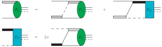
Figure 2: Feynman diagrams for the leading order coupled-channel homogeneous integral equations for the spectator functions, $F_{n}$ and $F_{D}$, of an S-wave $2n$-halo $D^{0}nn$ system. The solid (dashed) lines represent the neutron ($D^{0}$-meson) field. The gray (black) shaded thick lines represent the iterated $n$-$D^{0}$ ($n$-$n$) two-body S-wave T-matrix $\tau_{n}$ ($\tau_{D}$), Eq. (30), which in pionless EFT corresponds to the renormalized dressed dimer field propagator. The elliptical (rectangular) blobs represent the elastic (inelastic) channel $n+d_{(nD)}\to n+d_{(nD)}$ ($D^{0}+s_{(nn)}\to n+d_{(nD)}$) transition amplitude which is proportional to the spectator function $F_{n}$ ($F_{D}$) in the vicinity of trimer pole energy.

$$\begin{bmatrix}F_{n}\\ F_{D}\end{bmatrix}=\begin{bmatrix}\mathcal{K}_{nn}&\mathcal{K}_{nD}\\ \mathcal{K}_{Dn}&0\end{bmatrix}\begin{bmatrix}F_{n}\\ F_{D}\end{bmatrix}\,,$$ (46)

with discretized incoming $q$ and outgoing $q^{\prime}$ relative momenta, the binding energy $B_{3}$ corresponds to the eigenvalue of the kernel matrix $\mathcal{K}_{ij}$ [constructed from Eqs. (III.4) and  (45)] of unity. For completeness, we include a brief description of the numerical methodology for determining the solutions to the integral equations in Appendix C. In the next section, we demonstrate how the eigen-solutions to the spectator functions $F_{n}$ and $F_{D}$ can be used to extract the various one- and two-body matter density form factors that determine the structural characteristic of a plausible halo-bound $D^{0}nn$ system. In what follows, we dwell upon establishing the connection between the current effective quantum mechanical framework and the standard LO ${}^{{\pi}\!\!\!/}$EFT approach in the analysis of the $D^{0}nn$ system Raha:2017ahu .

III.5 Faddeev equations with sharp momentum cut-off: An EFT connection

In Ref. Raha:2017ahu , the S-wave $D^{0}nn$ system was investigated for the manifestation of Efimov effects under the idealized zero coupling limit ansatz that eliminated sub-threshold $DN$ ($T=1$) decay channels in the charm sector, e.g., $\pi^{-}\Lambda_{c},\,\pi^{0}\Sigma_{c}^{0}$ and $\pi^{-}\Sigma_{c}^{+}$. In this scenario, the $D^{0}nn$ system is pictured as a three-particle $2n$-halo cluster, with the so-called Samba configuration Yamashita:2004pv , having two real-bound $n$-$D^{0}$ subsystems and a virtual-bound $n$-$n$ subsystem. The fact that the binary subsystems in ZCL develop large scattering lengths makes the $D^{0}nn$ system Efimovian in nature. Using the framework of ${}^{{\pi}\!\!\!/}$EFT Braaten:2004rn ; Kaplan:1996xu ; Kaplan:1998tg ; Kaplan:1998we ; Kaplan:1998sz ; vanKolck:1998bw at LO, qualitative features of three-body universality can be explored. The non-relativistic effective Lagrangian at LO, consistent with low-energy symmetries (P, C, T, and Galilean invariances), is constructed as the sum of one-, two- and three-body parts Raha:2017ahu :

$${\mathcal{L}}=\left[{\mathcal{L}}_{n}+{\mathcal{L}}_{D}\right]_{\rm 1-body}+\left[{\mathcal{L}}_{s(nn)}+{\mathcal{L}}_{d(nD)}\right]_{\rm 2-body}+{\mathcal{L}}_{\rm 3-body}\,,$$ (47)

with

$${\mathcal{L}}_{n}(x) = n^{\dagger}(x)\left[i\partial_{t}+\frac{\nabla^{2}}{2M_{n}}\right]n(x)+\cdots\,,$$ (48)

$${\mathcal{L}}_{D}(x) = D^{\dagger}(x)\left[i\partial_{t}+\frac{\nabla^{2}}{2yM_{n}}\right]D(x)+\cdots\,,$$ (49)

$${\mathcal{L}}_{s(nn)}(x) = -\,s_{(nn)}^{\dagger}(x)\left[i\partial_{t}+\frac{\nabla^{2}}{4M_{n}}-\Delta_{s(nn)}\right]s_{(nn)}(x)$$ (50)

$$\qquad-\,g_{2s}\left[s_{(nn)}^{\dagger}(x)\left(n^{T}(x)\,\hat{P}_{(nn)}^{(^{1}S_{0})}\,n(x)\right)+\mbox{\rm h.c.}\right]+\cdots\,,$$

$${\mathcal{L}}_{d(nD)}(x) = -\,d_{(nD)}^{\dagger}(x)\left[i\partial_{t}+\frac{\nabla^{2}}{2M_{n}(1+y)}-\Delta_{d(nD)}\right]d_{(nD)}(x)$$ (51)

$$\qquad-\,g_{2d}\left[d_{(nD)}^{\dagger}(x)\,n(x)\,D(x)+\mbox{\rm h.c.}\right]+\cdots\,,$$

and

$$\mathcal{L}_{\rm 3-body}(x) = -\,\frac{M_{n}g_{3}(\Lambda_{\rm reg})}{\Lambda_{\rm reg}^{2}}\Bigg{[}yg_{2d}^{2}\left\{d^{T}_{(nD)}(x)\,\hat{P}^{(^{1}S_{0})}_{(nd)}\,n(x)\right\}^{\dagger}\left\{d^{T}_{(nD)}(x)\,\hat{P}^{(^{1}S_{0})}_{(nd)}\,n(x)\right\}$$

$$\hskip 71.13188pt+\,2g_{2s}g_{2d}\left\{d^{T}_{(nD)}(x)\,\hat{P}^{(^{1}S_{0})}_{(nd)}\,n(x)\right\}^{\dagger}\left\{s_{(nn)}(x)\,D(x)\right\}+{\rm h.c.}\Bigg{]}+\cdots\,,$$

where the ellipses are used to denote two- and three-body derivative interactions which by power counting contribute at subleading orders. For details on the ${}^{{\pi}\!\!\!/}$EFT power counting, we refer the reader to Refs. Braaten:2004rn ; Kaplan:1996xu ; Kaplan:1998tg ; Kaplan:1998we ; Kaplan:1998sz ; vanKolck:1998bw . In the above expressions as explicit degrees of freedom one includes the neutron field $n(x)$ and $D^{0}$-meson field $D(x)$ as the elementary fields of the theory, whose kinetic parts constitute the one-body terms of the effective Lagrangian. Here again for convenience we express the $D^{0}$-meson mass in terms of the neutron mass, namely, $M_{D}=yM_{n}$. In view of the existence of bound or anti-bound binary subsystems, it is customary in ${}^{{\pi}\!\!\!/}$EFT to introduce the unitarized auxiliary composite fields called dimerons Braaten:2004rn ; Bedaque:1998mb ; Bedaque:1998kg ; Bedaque:1999ve ; Bedaque:1998km ; Birse:1998dk ; Beane:2000fi ; Ando:2004mm ; Kaplan:1996nv , namely, the spin singlet $n$-$n$ di-neutron field $s_{(nn)}(x)$, and the spin-doublet $n$-$D^{0}$ dihadron field $d_{(nD)}(x)$. The corresponding renormalized dressed propagators (cf. Fig. 3) are given as

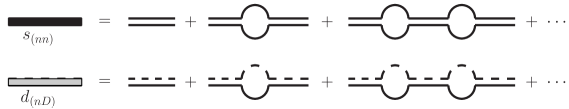
Figure 3: Renormalized dressed dimeron propagators associated with the $n$-$n$ and $n$-$D^{0}$ subsystems. The solid (dashed) lines represent the neutron ($D^{0}$-meson) field.

$$iS^{R}_{d}\left(l_{0},{\bf l}\right) = i\left[\frac{1}{a_{nD}}-\sqrt{\frac{y}{y+1}\left(-2M_{n}l_{0}+\frac{{\bf l}^{2}}{y+1}-i0_{+}\right)}-i0_{+}\right]^{-1}\,,\quad\text{and}$$

$$iS^{R}_{s}\left(l_{0},{\bf l}\right) = i\left[\frac{1}{a_{nn}}-\sqrt{-M_{n}l_{0}+\frac{{\bf l}^{2}}{4}-i0_{+}}-i0_{+}\right]^{-1}\,,$$ (53)

where $l\equiv(l_{0},{\bf l})$ is the lab-frame four-momentum of the dimeron fields. Equivalently, in the three-body center-of-mass frame, the above propagators can be re-expressed in terms of the Jacobi momentum $q=|\bf q|$ and the total three-body energy $z=E+i0_{+}$, after subtracting the respective kinetic energy of the spectator particle:

$$iS^{R}_{d}\left(z-\frac{q^{2}}{2M_{n}},{\bf q}\right) = i\left[\frac{1}{a_{nD}}-\sqrt{\frac{y}{y+1}\left(-2M_{n}z+\frac{y+2}{y+1}q^{2}-i0_{+}\right)}-i0_{+}\right]^{-1}\,,\quad\text{and}$$

$$iS^{R}_{s}\left(z-\frac{q^{2}}{2yM_{n}},{\bf q}\right) = i\left[\frac{1}{a_{nn}}-\sqrt{-M_{n}z+\frac{y+2}{4y}q^{2}-i0_{+}}-i0_{+}\right]^{-1}\,.$$ (54)

The ${}^{1}S_{0}$ projection operators in the respective spin channels are given in terms of the Pauli matrix $\sigma_{2}$:

$$\hat{P}_{(nn)}^{(^{1}S_{0})}=-i\frac{1}{2}\sigma_{2}\,\qquad\text{and}\qquad\hat{P}_{(nd)}^{(^{1}S_{0})}=-i\frac{1}{\sqrt{2}}\sigma_{2}\,.$$ (55)

The parameters $\Delta_{s(nn)}$ and $\Delta_{d(nK)}$ are proportional to the respective mass differences between the corresponding dimers and their constituent particles. The couplings $g_{2s}$ and $g_{2d}$ denote the LO two-body contact interactions in the spin-singlet and spin-doublet channels, respectively. These four quantities constitute the S-wave parameters of the LO two-body Lagrangian which can be fixed as follows:

$$g^{2}_{2s}=\frac{4\pi}{M_{n}}\,, g^{2}_{2d}=\frac{2\pi}{\mu_{nD}}\,,$$

$$\Delta_{s(nn)}+\frac{M_{n}g^{2}_{2s}}{2\pi^{2}}=\frac{1}{a_{nn}}\,, \text{and}\quad\Delta_{d(nD)}=\frac{1}{a_{nD}}\,,$$ (56)

where $a_{nn}=-18.63$ fm Chen:2008zzj is the phenomenologically extracted spin-singlet $nn$ S-wave scattering length, and $a_{nD}=4.141$ fm is the spin-doublet $D^{0}n$ S-wave scattering length in the ZCL scenario Raha:2017ahu . The latter value was extracted from the dynamical coupled-channel model analysis with vanishing couplings to $D^{0}n$ sub-threshold decay channels. It is notable that the “wrong signs” in front of the kinetic operators for the composite dimeron fields are indicative of their quasi-particle nature. Besides, these signs also ensure that corresponding effective ranges remain positive. The LO three-body Lagrangian (also referred to as the three-body force or 3BF for short) with the cut-off $\Lambda_{\rm reg}$-dependent contact coupling, $g_{3}=g_{3}(\Lambda_{\rm reg})$, is introduced for renormalization of the two-body STM equations. The value of $g_{3}$ which is a priori unknown in the theory is fixed via a three-body datum, e.g., one of the $D^{0}nn$ three-body level energies $B_{3}$ or the corresponding S-wave scattering length $a_{3}$. Unfortunately, there is no evidence whether $D^{0}nn$ forms any bound state, with neither $B_{3}$ nor $a_{3}$ known currently. Therefore, the predictability of the theory at present hinges solely upon guesstimating these quantities based on plausibility arguments. Once $g_{3}$ is fixed, other low-energy observables, such as the matter density form factors and their corresponding mean square radii, can readily be predicted.

With the above-mentioned components of ${}^{{\pi}\!\!\!/}$EFT, it is straightforward to use Feynman diagram techniques to obtain a set of two inhomogeneous coupled STM integral equation for the $D^{0}nn$ system. These represent the multiple scattering series in the elastic ($n+d_{(nD)}\to n+d_{(nD)}$) and inelastic ($D^{0}+s_{(nn)}\to n+d_{(nD)}$) scattering channels (denoted by the subscripts $a$ and $b$), as described in terms of the respective half-off-shell transition amplitudes Raha:2017ahu :

$$\mathcal{T}_{n}(p,q;E)\equiv t_{a}(p,q;E)\,,\quad\text{and}\quad\mathcal{T}_{D}(p,q;E)\equiv\sqrt{2}t_{b}(p,q;E)\,.$$

However, to look for Efimov trimers, the corresponding homogeneous equations are needed to be solved for non-trivial eigen-solutions $E=-B_{3}$ with a given UV cut-off $\Lambda_{\rm reg}$. The solutions correspond to the poles in the scattering amplitudes with residues that factorize into dimensionless spectator functions of the Jacobi momenta $p$ and $q$:

$$\mathcal{T}_{n}(p,q;E)\stackrel{{\scriptstyle E\,\to\,-B_{3}}}{{\approx}}\frac{F_{n}(p)F_{n}(q)}{E+B_{3}}\,,\quad\text{and}\quad\mathcal{T}_{D}(p,q;E)\stackrel{{\scriptstyle E\,\to\,-B_{3}}}{{\approx}}\frac{F_{D}(p)F_{D}(q)}{E+B_{3}}\,.$$ (57)

By invoking the above separable ansatz, we can reduce the two-variable STM equations into a single-variable coupled integral equations (in the Jacobi momentum $q$) described by the spectator functions.

In order to see the equivalence between the Faddeev-type and STM integral equations, we note that in LO EFT the effective potentials of the form, Eq. (23), simply correspond to zero-range contact interactions which vanish for momenta larger than the cut-off scale $\Lambda_{\rm reg}$. With the regulator functions $\chi(p)$ set as the Heaviside step function, the two-body T-matrix elements are readily evaluated analytically (cf. Appendix-B). Consequently, the UV limit of the loop integrations gets replaced by the finite cut-off $\Lambda_{\rm reg}$ defined by the step function. Now, it is easy to check that for large values of the cut-off, $\Lambda_{\rm reg}\rightarrow\infty$, both the inverse tangent functions in the T-matrices [cf. Eq. (30)] approach $\pi/2$. As a result, the T-matrices reduce to the standard renormalized two-body scattering amplitudes proportional to the renormalized dressed dimeron propagators:

$$\tau_{n}(q;B_{3}) = \frac{y+1}{\pi yM_{n}}\bigg{[}-\frac{1}{a_{nD}}+\gamma_{n}(q;B_{3})\bigg{]}^{-1}\equiv-\frac{y+1}{\pi yM_{n}}S^{R}_{d}\left(-B_{3}-\frac{q^{2}}{2M_{n}},{\bf q}\right)\,,\quad\text{and}$$

$$\tau_{D}(q;B_{3}) = \frac{2}{\pi M_{n}}\bigg{[}-\frac{1}{a_{nn}}+\gamma_{D}(q;B_{3})\bigg{]}^{-1}\equiv-\frac{2}{\pi M_{n}}S^{R}_{s}\left(-B_{3}-\frac{q^{2}}{2yM_{n}},{\bf q}\right)\,.$$ (58)

Next, we focus on the coupled Faddeev integral equation for the spectator functions, Eq. (III.4), with the upper integration limits replaced by the finite cut-off $\Lambda_{\rm reg}$. In this case, the only $x\equiv\hat{\bf q}\cdot\hat{\bf q}^{\prime}$ dependence arises from the free three-body Green’s functions $\mathcal{G}^{(i)}_{0}$, Eq. (24). The integration over $x$ can be performed analytically to obtain a form analogous to the homogeneous part of the STM equation (without the 3BF terms) for the $D^{0}nn$ system obtained in LO ${}^{{\pi}\!\!\!/}$EFT Raha:2017ahu :

$$F_{n}(q) = -\frac{1}{\pi}\int_{0}^{\Lambda_{\rm reg}}{\rm d}{q^{\prime}}q^{\prime 2}\left[(y+1)\mathcal{K}_{(D)}(q,q^{\prime};B_{3})\,S^{R}_{d}\left(-B_{3}-\frac{q^{\prime 2}}{2M_{n}},{\bf q}^{\prime}\right)\,F_{n}(q^{\prime})\right.$$

$$\left.\hskip 85.35826pt+\,2\mathcal{K}_{(n)}(q,q^{\prime};B_{3})\,S^{R}_{s}\left(-B_{3}-\frac{q^{\prime 2}}{2yM_{n}},{\bf q}^{\prime}\right)\,F_{D}(q^{\prime})\right]\,,\quad\text{and}$$

$$F_{D}(q) = -\frac{2(y+1)}{\pi y}\int_{0}^{\Lambda_{\rm reg}}d{q^{\prime}}q^{\prime 2}\left[\mathcal{K}_{(n)}(q^{\prime},q;B_{3})\,S^{R}_{d}\left(-B_{3}-\frac{q^{\prime 2}}{2M_{n}},{\bf q}^{\prime}\right)\,F_{n}(q^{\prime})\right]\,,$$ (59)

where the kernel functions are given as

$$\mathcal{K}_{(D)}(q,q^{\prime};B_{3}) = \frac{1}{2qq^{\prime}}\ln\bigg{(}\frac{ayM_{n}B_{3}+q^{2}+q^{\prime 2}+aqq^{\prime}}{ayM_{n}B_{3}+q^{2}+q^{\prime 2}-aqq^{\prime}}\bigg{)}\,;\quad a=\frac{2}{y+1}\,,\quad\text{and}$$

$$\mathcal{K}_{(n)}(q,q^{\prime};B_{3}) = \frac{1}{2qq^{\prime}}\ln\bigg{(}\frac{M_{n}B_{3}+q^{2}+bq^{\prime 2}+qq^{\prime}}{M_{n}B_{3}+q^{2}+bq^{\prime 2}-qq^{\prime}}\bigg{)}\,;\quad b=\frac{y+1}{2y}\,.$$ (60)

Note that the notation for the above kernel functions is different from the spectator notation of the three-particle Green’s function $\mathcal{G}^{(i)}_{0}$, where $i$ represents the spectator particle index. Here, $\mathcal{K}_{(\gamma)}$ in fact represents the S-wave projected interaction kernel with the freely propagating exchanged particle $\gamma=n,D$ between dimers of two different re-arrangement channels.

Now, it is straightforward to include the LO 3BF terms which convert the single-particle exchange kernel functions, $\mathcal{K}_{(D)}$ and $\mathcal{K}_{(n)}$, into their renormalized counterparts, $\mathbb{K}^{R}_{(D)}$ and $\mathbb{K}^{R}_{(n)}$, respectively, [cf. Fig. 4], namely,

$$\mathcal{K}_{(\gamma)}(q,q^{\prime};B_{3})\longrightarrow\mathbb{K}^{R}_{(\gamma)}(q,q^{\prime},\Lambda_{\rm reg};B_{3})=\mathcal{K}_{(\gamma)}(q,q^{\prime};B_{3})-\frac{g_{3}(\Lambda_{\rm reg})}{\Lambda^{2}_{\rm reg}}\,;\quad\gamma=n,D\,,$$ (61)

so that the final form of coupled STM equations renormalized by the 3BF terms, or the so-called STM3 equations Braaten:2004rn , for the $D^{0}nn$ system becomes

$$F_{n}(q) = -\frac{1}{\pi}\int_{0}^{\Lambda_{\rm reg}}{\rm d}{q^{\prime}}q^{\prime 2}\left[(y+1)\,\mathbb{K}^{R}_{(D)}(q,q^{\prime},\Lambda_{\rm reg};B_{3})\,S^{R}_{d}\left(-B_{3}-\frac{q^{\prime 2}}{2M_{n}},{\bf q}^{\prime}\right)\,F_{n}(q^{\prime})\right.$$

$$\left.\hskip 85.35826pt+\,2\,\mathbb{K}^{R}_{(n)}(q,q^{\prime},\Lambda_{\rm reg};B_{3})\,S^{R}_{s}\left(-B_{3}-\frac{q^{\prime 2}}{2yM_{n}},{\bf q}^{\prime}\right)\,F_{D}(q^{\prime})\right]\,,\,\quad\text{and}$$

$$F_{D}(q) = -\frac{2(y+1)}{\pi y}\,\int_{0}^{\Lambda_{\rm reg}}d{q^{\prime}}q^{\prime 2}\left[\mathbb{K}^{R}_{(n)}(q,q^{\prime},\Lambda_{\rm reg};B_{3})\,S^{R}_{d}\left(-B_{3}-\frac{q^{\prime 2}}{2M_{n}},{\bf q}^{\prime}\right)\,F_{n}(q^{\prime})\right]\,.$$ (62)

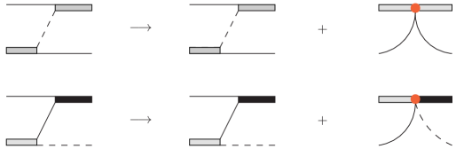
Figure 4: Feynman diagrams modifying the single $D^{0}$-meson and neutron exchange kernel functions, $\mathcal{K}_{(D)}$ and $\mathcal{K}_{(n)}$, respectively, into their renormalized versions, $\mathbb{K}^{R}_{(D)}$ and $\mathbb{K}^{R}_{(n)}$, contributing to the STM3 integral equations. The red-filled circles represent insertions of the regulator ($\Lambda_{\rm reg}$) dependent three-body contact interactions with coupling $g_{3}=g_{3}(\Lambda_{\rm reg})$.

In the asymptotic limit of the above equations, i.e., for $q,q^{\prime}\sim\Lambda_{\rm reg}\to\infty$, the 3BF terms do not contribute, in which case we find

$$F_{n}(q) = \frac{(1+y)^{2}}{2\pi\sqrt{y(2+y)}}\int^{\infty}_{0}\frac{{\rm d}q^{\prime}}{q}\ln\left(\frac{q^{2}+q^{\prime 2}+aqq^{\prime}}{q^{2}+q^{\prime 2}-aqq^{\prime}}\right)\,F_{n}(q^{\prime})$$

$$+\,\frac{1}{\pi}\sqrt{\frac{4y}{(2+y)}}\int^{\infty}_{0}\frac{{\rm d}q^{\prime}}{q}\ln\left(\frac{q^{2}+bq^{\prime 2}+qq^{\prime}}{q^{2}+bq^{\prime 2}-qq^{\prime}}\right)\,F_{D}(q^{\prime})\,,\quad\text{and}$$

$$F_{D}(q) = \frac{(1+y)^{2}}{\pi y\sqrt{y(2+y)}}\int^{\infty}_{0}\frac{{\rm d}q^{\prime}}{q}\ln\left(\frac{q^{\prime 2}+bq^{2}+qq^{\prime}}{q^{\prime 2}+bq^{2}-qq^{\prime}}\right)\,F_{n}(q^{\prime})\,,$$ (63)

Because the above asymptotic integrals are scale-free, the spectator functions must exhibit a power-law scaling behavior of the form $F_{i}(q)\propto q^{s-1}$. With this ansatz, the two coupled integral equations can be reduced into a single transcendental equation which must be numerically solved for determining the unknown exponent $s$:

$$1=C_{1}I_{0}(s;a)+C_{2}I_{1}(s;b)I_{2}(s;b)\,,$$ (64)

with the constants $C_{1,2}$ given by

$$C_{1}=\frac{(1+y)^{2}}{2\pi\sqrt{y(2+y)}}\,,\quad\text{and}\quad C_{2}=\frac{2(1+y)^{2}}{\pi^{2}y(2+y)}\,,$$ (65)

and the asymptotic integrals $I_{0,1,2}$ given by

$$I_{0}(s;a) = \int^{\infty}_{0}dx\,\,x^{s-1}\ln\left(\frac{1+x^{2}+ax}{1+x^{2}-ax}\right)=\frac{2\pi}{s}\frac{\sin\left[s\sin^{-1}\left(\frac{1}{2}a\right)\right]}{\cos\left(\frac{\pi}{2}s\right)}\,,$$

$$I_{1}(s;b) = \int^{\infty}_{0}dx\,\,x^{s-1}\ln\left(\frac{1+bx^{2}+x}{1+bx^{2}-x}\right)=\frac{2\pi}{s}\frac{1}{b^{s/2}}\frac{\sin\left[s\cot^{-1}\left(\sqrt{4b-1}\right)\right]}{\cos\left(\frac{\pi}{2}s\right)}\,,\quad\text{and}$$

$$I_{2}(s;b) = \int^{\infty}_{0}dx\,\,x^{s-1}\ln\left(\frac{b+x^{2}+x}{b+x^{2}-x}\right)=\frac{2\pi}{s}b^{s/2}\frac{\sin\left[s\cot^{-1}\left(\sqrt{4b-1}\right)\right]}{\cos\left(\frac{\pi}{2}s\right)}\,.$$ (66)

Solving the transcendental equation yields imaginary values of the parameter $s$, i.e., $s=\pm is^{\infty}_{0}$, with $s^{\infty}_{0}=1.02387...$ being a transcendental number. Thus, we infer that the $D^{0}nn$ system exhibits an RG limit cycle which formally suggests the Efimovian character of the system. The characteristic behavior stems from the discrete scale invariance of the system which is reflected in the asymptotic log-periodic running with periodicity governed by the factor $\lambda^{\infty}_{0}=\exp(\pi/s^{\infty}_{0})=21.5064...$ of the 3BF coupling $g_{3}=g_{3}(\Lambda_{\rm reg})$. The resulting cyclic singularities are well described by the analytical expression Bedaque:1998mb ; Bedaque:1998km ; Bedaque:1998kg ; Bedaque:1999ve

$$g_{3}(\Lambda_{\rm reg})\sim\aleph\,\frac{\sin\left[s^{\infty}_{0}\ln(\Lambda_{\rm reg}/\Lambda_{*})-\arctan(1/s^{\infty}_{0})\right]}{\sin\left[s^{\infty}_{0}\ln(\Lambda_{\rm reg}/\Lambda_{*})+\arctan(1/s^{\infty}_{0})\right]}\,,$$ (67)

where $\Lambda_{*}$ is a three-body parameter determined by a single low-energy observable, such as $B_{3}$. The numerical pre-factor $\aleph=0.870$ is introduced to improve the overall fit to the non-asymptotic data points. However, due to the paucity of information on whether the $D^{0}nn$ system is bound, the very best we can do in this scenario is to presume some reasonable values of the three-body binding energy for the shallowest (most excited) level state, say, $B_{T}=B_{3}-B_{nD}=0.1$ MeV and $1.0$ MeV (i.e., measured with respect to the 2+1 $nD^{0}$-dimer-particle break-up threshold energy of $B_{nD}=1.82$ MeV). This information is enough to determine the three-body coupling $g_{3}$ by solving the STM3 integral equations in the non-asymptotic kinematical domain. Figure 5 displays the cyclic singularities associated with the formation of successive three-body bound states, e.g., the ground $D^{0}nn$ state along with its first two excites states. In particular, the limit cycle nature of the 3BF thus obtained at the LO indicates the flexibility to choose the regulator scale $\Lambda_{\rm reg}$ in a suitable way that the 3BF terms effectively vanish. In other words, we may prefer to simply drop the 3BF terms and work with the STM equations by choosing a finite value of the cut-off that corresponds to one of the zeros of the limit cycle plot. The lowest value of such a cut-off, namely, $\Lambda_{\rm reg}=\Lambda^{(0)}_{\rm reg}$, may be identified with the (inverse) interaction range which sets the scale for the ground state or the deepest possible three-body binding energy of the system. Beyond this scale, all other deeper-level states get decoupled from the spectrum. In the following section, we revert back to the effective quantum mechanical formulation of the Faddeev equations, to demonstrate how the theoretical framework can be employed to assess the universal structural features of a plausible $D^{0}nn$ halo-bound system.

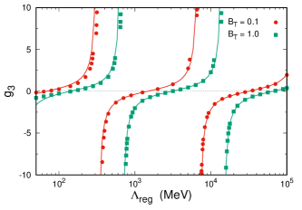
Figure 5: RG limit cycle for the three-body coupling $g_{3}$ of the $D^{0}nn$ system for two choices of the trimer binding energy, namely, $B_{T}=0.1$ and $1.0$ MeV (i.e., measured with respect to the $n$-$D^{0}$ dimer binding energy $B_{nD}=1.82$ MeV). The dotted and square data points correspond to the respective numerical solutions to the STM3 integral equations, while the solid lines denote the fitting curves using the asymptotic expression, Eq. (67), with the three-body fit parameter obtained as $\Lambda_{*}=31.8$ MeV and $66.2$ MeV.

IV Geometrical features of an Efimovian $D^{0}nn$ system

We now revisit the Faddeev equations which in conjunction with the LO halo-EFT formalism can also be used to determine low-energy observables, such as the one- and two-body matter density form factors and their corresponding root mean square radii, in view of a plausible halo-bound $D^{0}nn$ system. These observables can help unravel various universal structural features to assess the Efimov nature of the bound system. For this purpose, we need information on the full three-body wavefunction. Following the general methodology outlined in Refs. Canham:2008jd ; DL-Canham:2009 , we now demonstrate in the reconstruction of the full $D^{0}nn$ three-body wavefunctions from the solutions to the spectator functions $F_{n}$ and $F_{D}$ from Eq. (46). Subsequently, the wavefunctions are used to determine the form factors and matter radii.

IV.1 Reconstruction of three-body S-wave wavefunction at LO

The full three-body wavefunction is represented by the state which is the sum of the Faddeev partitions for the $D^{0}nn$ system:

$$|\Psi\rangle=|\psi_{n_{1}}\rangle+|\psi_{n_{2}}\rangle+|\psi_{D}\rangle=(1-\mathcal{P})|\psi_{n}\rangle+|\psi_{D}\rangle\,.$$ (68)

The form of the wavefunction depends not only on the choice of the binary subsystem but also on the corresponding spectator basis to represent the Jacobi momenta. Let us represent the S-wave projected part as

$${}_{i}\langle pq|\Psi\rangle\equiv\Psi_{i}(p,q)\,,$$ (69)

where index $i=n,D$ indicates the actual spectator particle. In other words, the same three-body wavefunction can be represented in two equivalent ways with respect to the two distinct fragmentation channels labeled by $n$ or $D$. With, say, $p\equiv p_{n_{2}}$ and $q\equiv q_{n_{2}}$, as the preferred choice of the Jacobi momentum representation with $n_{2}$ neutron as the spectator (cf. Channel-3 in Fig. 15), the full wavefunction can be written as

$$\Psi_{n_{2}}(p,q) = \,{}_{n_{2}}\langle pq|1-\mathcal{P}|\psi_{n_{2}}\rangle+\,{}_{n_{2}}\langle pq|\psi_{D}\rangle$$ (70)

$$= \psi_{n_{2}}(p,q)+\int{\rm d}p^{\prime}p^{\prime 2}{\rm d}q^{\prime}q^{\prime 2}\,{}_{n_{1}}\langle pq|p^{\prime}q^{\prime}\rangle_{n_{2}}\,\,\psi_{n_{2}}(p^{\prime},q^{\prime})$$

$$\hskip 35.56593pt+\,\int{\rm d}p^{\prime}p^{\prime 2}{\rm d}q^{\prime}q^{\prime 2}\,{}_{n_{2}}\langle pq|p^{\prime}q^{\prime}\rangle_{D}\,\,\psi_{D}(p^{\prime},q^{\prime})\,.$$

In the above equation, we again need to evaluate the overlap matrix elements as we have done in the previous section using the re-coupling constants $\mathscr{G}^{(nn)}=\mathscr{G}^{(nD)}=1/2$. The only difference with the previous case is that here we need to re-define/shift the $n_{2}$ neutron spectator Jacobi relative momenta $p^{\prime}\equiv p^{\prime}_{n_{2}}$ and $q^{\prime}\equiv q^{\prime}_{n_{2}}$ either into the basis of the $n_{1}$ neutron as the spectator or into the basis of the $D^{0}$-meson as the spectator Nogga:2001 . The results for the S-wave overlap matrix elements associated with Eq. (70) are

$${}_{n_{1}}\langle pq|p^{\prime}q^{\prime}\rangle_{n_{2}}\,\mathscr{G}^{(nn)} \equiv \frac{1}{2}\,{}_{n_{1}}\!\langle p_{n_{2}}q_{n_{2}}|p^{\prime}_{n_{2}}q^{\prime}_{n_{2}}\rangle_{n_{2}}=\frac{1}{2}\int_{-1}^{1}{\rm d}x\frac{\delta(p^{\prime}-\Pi_{nn})}{p^{\prime}\Pi_{nn}}\frac{\delta(q^{\prime}-\Pi^{\prime}_{nn})}{q^{\prime}\Pi^{\prime}_{nn}}\,,\quad\text{and}$$

$${}_{n_{2}}\langle pq|p^{\prime}q^{\prime}\rangle_{D}\,\mathscr{G}^{(nD)} \equiv \frac{1}{2}\,{}_{n_{2}}\!\langle p_{n_{2}}q_{n_{2}}|p^{\prime}_{n_{2}}q^{\prime}_{n_{2}}\rangle_{D}$$ (71)

$$= \frac{1}{2}\,{}_{D}\langle p_{D}q_{D}|p^{\prime}_{n_{2}}q^{\prime}_{n_{2}}\rangle_{D}=\frac{1}{2}\int_{-1}^{1}{\rm d}x\frac{\delta(p^{\prime}-\Pi_{nD})}{p^{\prime}\Pi_{nD}}\frac{\delta(q^{\prime}-\Pi^{\prime}_{nD})}{q^{\prime}\Pi^{\prime}_{nD}}\,,$$

where the shifted momenta for the above re-couplings are respectively given as

$$\Pi_{nn}(p,q;x) = \sqrt{\left(\frac{1}{y+1}\right)^{2}p^{2}+\frac{y^{2}(y+2)^{2}}{(y+1)^{4}}q^{2}+2\frac{y(y+2)}{(y+1)^{3}}\,pqx}\,,$$

$$\Pi^{\prime}_{nn}(p,q;x) = \sqrt{p^{2}+\left(\frac{1}{y+1}\right)^{2}q^{2}-2\left(\frac{1}{y+1}\right)pqx}\,,$$ (72)

and

$$\Pi_{nD}(p,q;x) = \sqrt{\frac{p^{2}}{4}+\frac{(y+2)^{2}}{4(y+1)^{2}}q^{2}+\frac{y+2}{2(y+1)}\,pqx}\,,$$

$$\Pi^{\prime}_{nD}(p,q;x) = \sqrt{p^{2}+\left(\frac{y}{y+1}\right)^{2}q^{2}-2\left(\frac{y}{y+1}\right)\,pqx}\,,$$ (73)

where $x\equiv\hat{\bf p}\cdot\hat{\bf q}$.

Using the above results, as well as the relations between the Faddeev components and the spectator functions, Eq. (44), yields the following expression for the full S-wave three-body wavefunction in the $i=n$ Jacobi channel after integrating over the delta functions:

$$\Psi_{n}(p,q) = \psi_{n}(p,q)+\frac{1}{2}\int_{-1}^{1}{\rm d}x\,\big{[}\psi_{n}(\Pi_{nn},\Pi^{\prime}_{nn})+\psi_{D}(\Pi_{nD},\Pi^{\prime}_{nD})\big{]}$$ (74)

$$= \mathcal{G}^{(n)}_{0}(p,q;B_{3})\bigg{[}\chi(p)\,\tau_{n}(q;B_{3})\,F_{n}(q)+\frac{1}{2}\int_{-1}^{1}{\rm d}x\,\chi\left(\Pi_{nn}\right)\,\tau_{n}(\Pi^{\prime}_{nn};B_{3})\,F_{n}(\Pi^{\prime}_{nn})$$

$$\hskip 65.44142pt+\,\frac{1}{2}\int_{-1}^{1}{\rm d}x\,\chi\left(\Pi_{nD}\right)\,\tau_{D}(\Pi^{\prime}_{nD};B_{3})\,F_{D}(\Pi^{\prime}_{nD})\bigg{]}\,,$$

where we have utilized the fact that

$$\mathcal{G}^{(n)}_{0}(\Pi_{nn},\Pi^{\prime}_{nn};B_{3})=\mathcal{G}^{(D)}_{0}(\Pi_{nD},\Pi^{\prime}_{nD};B_{3})=\mathcal{G}^{(n)}_{0}(p,q;B_{3})\,.$$

Next, with $p\equiv p_{D}$ and $q\equiv q_{D}$ as the preferred choice of the Jacobi momentum representation with $D^{0}$-meson as the spectator (cf. Channel-1 in Fig. 15), the full wavefunction can be written as

$$\Psi_{D}(p,q) = {}_{D}\langle pq|\psi_{D}\rangle+{}_{D}\langle pq|1-\mathcal{P}|\psi_{n_{1}}\rangle$$ (75)

$$= \psi_{D}(p,q)+2\int{\rm d}p\,p^{\prime 2}{\rm d}q^{\prime}\,q^{\prime 2}\,{}_{D}\langle pq|p^{\prime}q^{\prime}\rangle_{n_{1}}\,\psi_{n_{1}}(p^{\prime},q^{\prime})\,.$$

In the above equation, we need to evaluate the overlap matrix elements using the re-coupling factor $\mathscr{G}^{(Dn)}=1/2$. Here we need to re-define/shift the $D^{0}$ spectator Jacobi relative momenta $p^{\prime}\equiv p^{\prime}_{D}$ and $q^{\prime}\equiv q^{\prime}_{D}$ into the basis of the $n_{1}$ neutron as the spectator Nogga:2001 . The result of the S-wave overlap matrix element associated with Eq. (75) is

$${}_{D}\langle pq|p^{\prime}q^{\prime}\rangle_{n_{1}}\,\mathscr{G}^{(Dn)} = \frac{1}{2}\,{}_{D}\langle p_{D}q_{D}|p^{\prime}_{D}q^{\prime}_{D}\rangle_{n_{1}}$$ (76)

$$= \frac{1}{2}\,{}_{n_{1}}\!\langle p_{n_{1}}q_{n_{1}}|p^{\prime}_{D}q^{\prime}_{D}\rangle_{n_{1}}=\frac{1}{2}\int_{-1}^{1}{\rm d}x\frac{\delta(p^{\prime}-\Pi_{Dn})}{p^{\prime}\Pi_{Dn}}\frac{\delta(q^{\prime}-\Pi^{\prime}_{Dn})}{q^{\prime}\Pi^{\prime}_{Dn}}\,,$$

where the shifted momenta are given by

$$\Pi_{Dn}(p,q;x) = \sqrt{\left(\frac{y}{y+1}\right)^{2}p^{2}+\frac{(y+2)^{2}}{4(y+1)^{2}}q^{2}+\frac{y(y+2)}{(y+1)^{2}}pqx}\,,\quad\text{and}$$

$$\Pi^{\prime}_{Dn}(p,q;x) = \sqrt{p^{2}+\frac{q^{2}}{4}-pqx}\,.$$ (77)

Substituting the above result for the overlap matrix element ${}_{D}\langle pq|p^{\prime}q^{\prime}\rangle_{n}$ in Eq. (75), then inserting the relations between the Faddeev components and spectator functions, and finally performing the delta function integrations, we obtain the following expression for the full S-wave three-body wavefunction in the $i=D$ fragmentation channel:

$$\Psi_{D}(p,q) = \mathcal{G}^{(D)}_{0}(p,q;B_{3})\,\chi(p)\,\tau_{D}(q;B_{3})\,F_{D}(q)$$

$$\quad+\,\int_{-1}^{1}{\rm d}x\,\mathcal{G}^{(n)}_{0}(\Pi_{Dn},\Pi^{\prime}_{Dn};B_{3})\,\chi\left(\Pi_{Dn}\right)\,\tau_{n}(\Pi^{\prime}_{Dn};B_{3})\,F_{n}(\Pi^{\prime}_{Dn})$$

$$= \mathcal{G}^{(D)}_{0}(p,q;B_{3})\,\bigg{[}\chi(p)\,\tau_{D}(q;B_{3})\,F_{D}(q)+\int_{-1}^{1}{\rm d}x\,\chi\left(\Pi_{Dn}\right)\,\tau_{n}(\Pi^{\prime}_{Dn};B_{3})\,F_{n}(\Pi^{\prime}_{Dn})\bigg{]}\,,$$

where we have utilized the fact that

$$\mathcal{G}^{(n)}_{0}(\Pi_{Dn},\Pi^{\prime}_{Dn};B_{3})=\mathcal{G}^{(D)}_{0}(p,q;B_{3})\,,$$

and also employed the Heaviside step function regulator, $\chi(p)=\Theta(\Lambda_{\rm reg}-p)$. Furthermore, we used the two-body T-matrices $\tau_{n}$ and $\tau_{D}$ from Eq. (30), the free three-body propagator functions $\mathcal{G}^{(n)}_{0}$ and $\mathcal{G}^{(D)}_{0}$ from Eq. (24), and finally, evaluated the spectator functions $F_{n}$ and $F_{D}$ from the matrix equation, Eq. (46), either at the relative on-shell momentum $q$ or at a shifted off-shell momentum $q^{\prime}=\Pi^{\prime}(p,q)$. The reconstructed full three-body wavefunctions $\Psi_{n}$ and $\Psi_{D}$ at LO with respect to the two fragmentation channels $i=n,D$ are illustrated via the Feynman diagrams in Fig. 6.

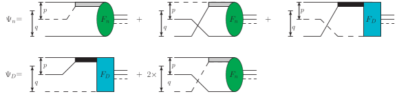
Figure 6: Reconstruction of the full three-body S-wave wavefunctions $\Psi_{i}(p,q)$ at LO with respect to the $i=n,D$ fragmentation channels in Jacobi representation for the $D^{0}nn$ system. The solid/dashed lines denote the neutron/$D^{0}$-meson propagators. The rectangular/oval blobs represent the three-body scattering kernels associated with the spectator functions $F_{i}(q)$. The gray/black thick-shaded thick lines represent the iterated $n$-$D^{0}$/$n$-$n$ two-body S-wave T-matrices $\tau_{i}$, Eq. (58), which in the EFT framework are interpreted as renormalized dressed auxiliary field propagators.

IV.2 Matter Density Form Factors and their radii

With the full three-body wavefunction, Eqs. (74) and (LABEL:eq:Psi_D_pq), determined, we are now in a position to determine the matter density form factor and their corresponding radii. In Jacobi momentum representation, the S-wave matter density form factors are obtained by calculating the S-wave projected Fourier transforms of the respective matter densities with respect to the squares of the three-momentum transfer ${\bf k}$. They are symbolized by the normalized functions $\mathcal{F}_{i}(k^{2}=0)=1$ and $\mathcal{F}_{ni}(k^{2}=0)=1$, where $i=n,D$, depending on the fragmentation channel. The expression for the S-wave one-body matter density form factors is given by

$$\mathcal{F}_{i}(k^{2})=\int{\rm d}p\,p^{2}\int{\rm d}q\,q^{2}\int_{-1}^{1}{\rm d}\xi\,\widetilde{\Psi}_{i}(p,q)\,\widetilde{\Psi}_{i}(p,\sqrt{q^{2}+k^{2}-2qk\xi})\,,\quad i=n,D\,,$$ (79)

where $\xi\equiv\hat{\bf k}\cdot\hat{\bf q}$, and $\widetilde{\Psi}_{i}(p,q)$ represents the S-wave projected part of the complete three-body normalized wavefunction $\Psi_{i}({\bf p},{\bf q})$ in three-dimension, namely,

$$\widetilde{\Psi}_{i}(p,q)=\frac{1}{4\pi}\int{\rm d}\Omega_{\hat{p}}\int{\rm d}\Omega_{\hat{q}}\,\widetilde{\Psi}_{i}({\bf p},{\bf q})\,P_{0}(\hat{\bf p}\cdot\hat{\bf q})\,,\quad\text{with}$$

$$\widetilde{\Psi}_{i}({\bf p},{\bf q})=\frac{\Psi_{i}({\bf p},{\bf q})}{\displaystyle{\sqrt{\int{\rm d}^{3}{\bf p}\int{\rm d}^{3}{\bf q}\,\Psi^{2}_{i}({\bf p},{\bf q})}}}\,,\quad i=n,D\,.$$ (80)

For the purpose of illustration, in Fig. 7 we display the corresponding momentum-space radial probability densities as functions of the Jacobi momenta $p$ and $q$, where the normalized probability densities are defined as

$$P_{i}(p,q)=\frac{\displaystyle{p^{2}q^{2}\,\Psi^{2}_{i}(p,q)}}{\displaystyle{\int{\rm d}{p}\,p^{2}\int{\rm d}{q}\,q^{2}\,\Psi^{2}_{i}(p,q)}}\,,\quad i=n,D\,.$$ (81)

Next, the expressions for the S-wave two-body matter form factors are given by

$$\mathcal{F}_{nD}(k^{2}) = \int{\rm d}p\,p^{2}\int{\rm d}q\,q^{2}\int_{-1}^{1}{\rm d}\zeta\,\widetilde{\Psi}_{n}(p,q)\,\widetilde{\Psi}_{n}(\sqrt{p^{2}+k^{2}-2pk\zeta},q)\,,\quad\text{and}$$

$$\mathcal{F}_{nn}(k^{2}) = \int{\rm d}p\,p^{2}\int{\rm d}q\,q^{2}\int_{-1}^{1}{\rm d}\zeta\,\widetilde{\Psi}_{D}(p,q)\,\widetilde{\Psi}_{D}(\sqrt{p^{2}+k^{2}-2pk\zeta},q)\,,$$ (82)

where $\zeta\equiv\hat{\bf k}\cdot\hat{\bf p}$. The one- and two-body form factors defined above constitute the basis for determining the universal geometrical structure of the putative S-wave $2n$-halo-bound $D^{0}nn$ system.

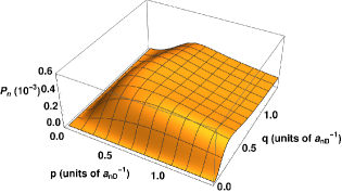
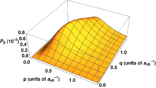
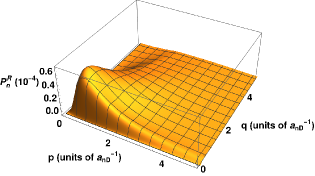
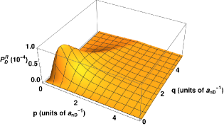
Figure 7: Normalized momentum-space S-wave radial probability densities, Eq. (81) corresponding to the $D^{0}nn$ ground state full three-body wavefunctions $\Psi_{n}(p,q)$ and $\Psi_{D}(p,q)$ at LO, with input binding energy $B_{T}=B_{3}-B_{nD}=0.1$ MeV. Upper panel: Unrenormalized densities at the cut-off scale $\Lambda_{\rm reg}\simeq 68$ MeV, corresponding to the input value of $B_{3}$. Lower panel: Renormalized asymptotic densities as $\Lambda_{\rm reg}\to\infty$. The Jacobi momenta $p$ and $q$ are expressed in units of the inverse S-wave $n$-$D^{0}$ scattering length or $nD^{0}$-dimer binding momentum, i.e., $\gamma_{nD}\sim a^{-1}_{nD}=47.65$ MeV.

We can now extract the mean square two-particle distances between pairs of individual particles, namely, $\langle r^{2}_{nn}\rangle$ and $\langle r^{2}_{Dn}\rangle$, as well as the mean square distances between a spectator particle and the center-of-mass of the binary subsystem, namely, $\langle r^{2}_{n-nD}\rangle$ and $\langle r^{2}_{D-nn}\rangle$. These radii are obtained from the slopes of the one- and two-body form factors at $k^{2}\equiv|{\bf k}|^{2}=0$. The different matter radii for the $D^{0}nn$ system are illustrated in Fig. 8. The slopes of $\mathcal{F}_{ni}$ give the information regarding the mean square two-particle distances $\langle r^{2}_{nn}\rangle$ and $\langle r^{2}_{nD}\rangle$ for the $n$-$n$ and $n$-$D^{0}$ binary subsystems, respectively. Whereas, the slope of $\mathcal{F}_{n}$ ($\mathcal{F}_{D}$) is related to the mean square distance $\langle r^{2}_{n-nD}\rangle$ ($\langle r^{2}_{D-nn}\rangle$) between the spectator neutron ($D^{0}$-meson) and the center-of-mass of the $n$-$D^{0}$ ($n$-$n$) subsystem. This information can further be utilized to obtain the mean square distances $\langle r^{2}_{i}\rangle$ of the distinct bound particles $i=n,D$ from the center-of-mass of the bound $D^{0}nn$ system using the relation Canham:2008jd :

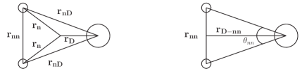
Figure 8: The matter radii defining the geometrical structure of a $2n$-halo bound $D^{0}nn$ system.

$$\langle r^{2}_{i}\rangle=-6\left(\frac{{\rm d}\mathcal{F}_{i}(k^{2})}{{\rm d}k^{2}}\right)_{k^{2}=0}\bigg{[}1-\frac{M_{i}}{(2+y)M_{n}}\bigg{]}^{2}\,,\;\quad i=n,D\,,$$ (84)

where $M_{i}$ refers to the mass of the bound particle in question whose mean square distance is needed to be determined. Similarly, one can define an effective/mean geometrical matter radius for the $2n$-halo bound $D^{0}nn$ system with a point-like core Hammer:2017tjm :

$$\langle r^{2}_{\rm eff}\rangle_{\rm 2n-halo}=\frac{2(y+1)^{2}}{(y+2)^{3}}\langle r^{2}_{n-nD}\rangle+\frac{4y}{(y+2)^{3}}\langle r^{2}_{D-nn}\rangle\,.$$ (85)

Finally, it is a matter of simple geometry to determine the $n-D^{0}-n$ opening angle Canham:2008jd ; Acharya:2013aea :

$$\theta_{nn}=2\arctan\sqrt{\frac{\langle r^{2}_{nn}\rangle}{4\langle r^{2}_{D-nn}\rangle}}\,.$$ (86)

A numerical estimation of the aforementioned observables helps to reconstruct a two-dimensional geometrical structure of the $D^{0}nn$ system, as we provide in the next section.

V Results and Discussion

In this section, we shall display the results of our LO analysis of the S-wave $2n$-halo $D^{0}nn$ system. Here, we mainly focus on the estimation of the universal geometrical features for a plausible trimer state under the idealized ZCL scenario Raha:2017ahu . For our numerical analysis, we prefer the sharp momentum cut-off regularization scheme, as incorporated via the Heaviside step function in the two-body T-matrices and the wavefunctions kernels. The numerical values of the particle masses used in our calculations are displayed in Table 3. The sole two-body input parameters in our effective theory are the S-wave scattering lengths $a_{nD}=4.141$ fm Raha:2017ahu and $a_{nn}=-18.63$ Chen:2008zzj . In Fig. 9 (left panel) we display the sequence of geometrically spaced Efimov states which progressively emerge above the $D^{0}n+n$ dimer-particle break-up threshold energy $B_{nD}=1.82$ MeV upon increasing the cut-off momentum $\Lambda_{\rm reg}$. The binding energies represent the non-trivial solutions to the homogeneous STM equations, Eq. (III.5), without the 3BF terms. The values of the critical cut-offs $\Lambda_{\rm reg}=\Lambda^{(m)}_{\rm crit}$ corresponding to the three shallowest Efimov level states are $\Lambda^{(m=0)}_{\rm crit}\approx 48$ MeV, $\Lambda^{(m=1)}_{\rm crit}\approx 1122$ MeV, and $\Lambda^{(m=2)}_{\rm crit}\approx 23932$ MeV, as consistent with the LO ${}^{\pi\!\!\!\!/}$EFT analysis of Ref. Raha:2017ahu . The small value of the critical cut-off for the ground state relative to the ${}^{\pi\!\!\!\!/}$EFT breakdown scale ($m_{\pi}$) is suggestive of a plausible Efimovian $D^{0}nn$ system which may either survive as a realistic exotic nuclei or evolve into a quasi-bound system upon relaxation of the ZCL scenario. Whereas, the deeper level states emerging at scales substantially larger than $m_{\pi}$ are naturally excluded from the low-energy EFT description. The sensitive dependence of the three-body binding energy on the regulator scale, as seen in Fig. 9 (right panel), can nonetheless be renormalized by introducing the regulator-dependent 3BF terms via the STM3 equations, Eq. (62). The corresponding couplings require three-body data to uniquely determine their RG running, namely, $g_{3}=g_{3}(\Lambda_{\rm reg})$. However, such phenomenological information is currently unavailable. Thus, for instance by fixing an ad hoc near-threshold value of the binding energy of the shallowest (most excited) Efimov level, say, $B_{3}=1.92$ MeV (i.e., $B_{T}=B_{3}-B_{nD}=0.1$ MeV, where the $B_{nD}=1.82$ MeV is $D^{0}n+n$ dimer-particle threshold energy), the limit cycle nature of $g_{3}$ can be predicted by solving the STM3 equations [cf. Fig. 5]. Subsequently, regulator-independent values of all the deeper-level energies can then be readily predicted by the STM3 equations with the coupling $g_{3}$ already determined by the limit cycle. The result is illustrated in the right panel of the Fig. 9, where the two deepest-level energies $B_{T}\approx 73$ MeV and $B_{T}\approx 29934$ MeV are yielded as predictions.

Particle	Mass Symbol	Numerical Value (MeV)
$D^{0}$-Meson	$M_{D}$	1864.3
Neutron ($n$)	$M_{n}$	939.565

Table 3: PDG Zyla:2020zbs values of particle masses used in the calculation.

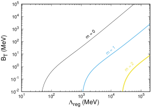
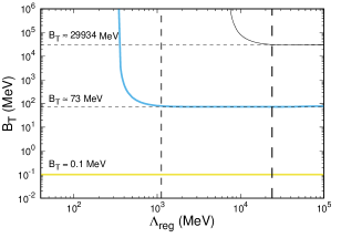
Figure 9: Cut-off scale ($\Lambda_{\rm reg}$) dependence of the $D^{0}nn$ trimer binding energy $B_{T}=B_{3}-B_{nD}$, (where the $B_{nD}=1.82$ MeV is $D^{0}n+n$ dimer-particle threshold energy) obtained as a nontrivial solution to the Faddeev integral equations at leading order. Here we display three sets of curves corresponding to the ground ($m=0$) and the first two excited trimer ($m=1,2$) states. Left panel: Solutions obtained using the unrenormalized STM equations without the 3BF terms. Right panel: Solutions obtained using the STM3 equations renormalized by the three-body couplings $g_{3}=g_{3}(\Lambda_{\rm reg})$ fixed by the RG limit cycle behavior [cf. Fig. 5]. Fixing the trimer binding energy $B_{T}=0.1$ MeV for the shallowest Efimov level, the regulator independent eigenenergies $B_{T}=73$ MeV and $B_{T}=29934$ MeV are yielded as predictions.

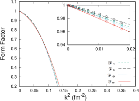
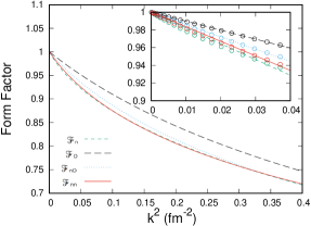
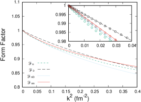
Figure 10: Leading order S-wave one- and two-body matter density form factors for the $D^{0}nn$ system as a function of squared three-momentum transfer $k^{2}$ for the ground ($m=0$) state trimer with a three-body binding energy $B_{T}=2.0$ MeV (upper left panel), and for the first two excited ($m=1,2$) state trimers, each corresponding to the fixed binding energy $B_{T}=0.18$ MeV (upper right and lower panels). All form factors are normalized to unity at $k^{2}=0$. The inset plots depict the linear fits to our numerical data points for very low momentum transfers. These results all correspond to the two-body inputs in the ZCL scenario Raha:2017ahu .

Next, assuming that the S-wave $D^{0}nn$ system is halo-bound, we present our results pertaining to its Samba structure Yamashita:2004pv . In Fig. 10, we plot the various LO S-wave one- and two-body matter density form factors for the ground ($m=0$) and the first two excited ($m=1,2$) trimer states for the $D^{0}nn$ system. Here, we demonstrate our numerical results by fixing a small ad hoc value of the three-body binding energy, say, $B_{3}=2.0$ MeV (i.e., $B_{T}=0.18$ MeV) for the first two ($m=1,2$) excited states, corresponding to $\Lambda_{\rm reg}\approx 1.3$ GeV ($1.7$ GeV) for the first ($m=1$) excited state and $\Lambda_{\rm reg}\approx 31$ GeV ($36$ GeV) for the second ($m=2$) excited state (despite barely qualifying as realizable Efimov states given the large critical cut-offs at which they appear above the threshold, see left panel of Fig. 9). As for the ground ($m=0$) state, we prefer to demonstrate our form factor results for a somewhat larger value of the three-body binding energy, say, $B_{3}=3.82$ MeV (i.e., $B_{T}=2.0$ MeV), lest numerical artifacts arise in the small cut-off region. The non-linear nature of the form factors is evident over a substantial range of low-momentum transfers, say, up to the pion mass ($k^{2}\equiv|{\bf k}|^{2}\lesssim m^{2}_{\pi}$). However, in the $k^{2}\sim 0$ region they may be considered approximately linear with constant slopes, which in turn determine the corresponding mean squared radii. We find that the ground state form factors look significantly different from those of the excited states. Such differences in the character of the unrenormalized results (i.e., those obtained excluding the 3BF) are naturally anticipated, given the fact that only very shallow (near-threshold) trimer states with $B_{T}\to 0$ (however, with the regulator substantially larger than $m_{\pi}$) occur within the region of the universality of the Efimov spectrum. With the binding momenta and regulator cut-offs of comparable size, our ground state results are likely to be plagued by poor numerical convergence in the small cut-off region. Hence, for a more robust prediction, it is desirable to compare the results for a different regularization scheme, such as the Gaussian scheme. This would, however, require us to re-determine the corresponding 3BF RG limit cycle in the adopted regularization, which may, in principle, be different from the sharp cut-off scheme, Fig. 5. Such a comparative study shall be undertaken in a future work.

Efimov level $m$	$B_{3}$ (MeV)	$\Lambda_{\rm reg}$ (MeV)	(1) $r_{nn}$	(2) $r_{nD}$	(3) $r_{n}$	(4) $r_{D}$	(5) $r_{n-nD}$	(6) $r_{D-nn}$	$\theta_{nn}$
	1.92	67.9	13.2	12.6	6.9	3.1	12.7	11.5	59.70
	2.00	78.6	10.6	10.0	5.5	2.7	10.1	9.3	59.51
$m=0$	2.50	123.8	5.9	5.5	3.3	1.8	5.4	5.1	60.72
(Ground)	3.00	157.7	4.4	4.1	2.6	1.5	4.0	3.7	62.22
	3.82	204.1	3.3	3.1	2.2	1.3	3.0	2.7	63.03
	4.00	213.1	3.2	2.9	2.0	1.2	2.8	2.6	63.08
	1.92	1473	3.5	3.1	3.7	1.4	3.9	2.7	66.58
	2.00	1681	3.1	2.8	2.7	1.3	3.2	2.4	64.72
$m=1$	2.50	2608	2.1	2.1	1.5	0.9	2.0	1.8	59.46
(First excited)	3.00	3327	1.7	1.8	1.2	0.8	1.6	1.6	57.33
	3.82	4320	1.4	1.5	1.0	0.7	1.3	1.3	55.50
	4.00	4519	1.4	1.4	1.0	0.7	1.3	1.3	55.23
	1.92	31467	2.2	2.2	2.5	0.9	2.4	1.9	61.43
	2.00	35935	2.0	2.0	1.9	0.9	2.1	1.7	59.59
$m=2$	2.50	55878	1.4	1.5	1.1	0.7	1.4	1.4	55.11
(Second excited)	3.00	71328	1.2	1.3	0.9	0.6	1.2	1.2	53.40
	3.82	92700	1.0	1.1	0.7	0.5	1.0	1.0	52.02
	4.00	96961	1.0	1.1	0.7	0.5	1.0	1.0	51.82

Table 4: Various leading order root mean squared radii $r_{1,...,6}\equiv\sqrt{\langle r^{2}_{1,...,6}\rangle}$ (in fm) and the $n-D^{0}-n$ opening angle $\theta_{nn}$ (in degrees) for a halo-bound S-wave $D^{0}nn$ system. The results are displayed for the ground ($m=0$) and the first two excited ($m=1,2$) Efimov state trimers. The results are obtained using a sharp momentum cut-off regulator $\Lambda_{\rm reg}$. The results correspond to two-body inputs in the ZCL model scenario of Ref. Raha:2017ahu .

With the three lowest trimer ($m=0,1,2$) state form factors evaluated for various input $B_{3}\,(\text{or }B_{T})$ values at specific $\Lambda_{\rm reg}$, as determined by Fig. 9, we first study the regulator dependence of the different root mean squared (rms) distances defining the geometrical structure of $D^{0}nn$. Employing Eqs. (83) and (84), we summarize the corresponding results in Table 4. The inter-particle rms distance between the $(ij)$-pair is defined as $r_{ij}\equiv\sqrt{\langle r^{2}_{ij}\rangle}$. The rms distance of the spectator particle $i$ from the center-of-mass of the binary subsystem $j$-$k$ is defined as $r_{i-{jk}}\equiv\sqrt{\langle r^{2}_{i-{jk}}\rangle}$. Finally, the rms distance of the particle $i$ from the three-body center-of-mass is defined as $r_{i}\equiv\sqrt{\langle r^{2}_{i}\rangle}$. As evident from the table, with the increase of $B_{3}$ for the trimer levels, the magnitude of all the rms radii decreases. This is naturally anticipated because stronger the binding of a given level, the more compact it gets. Especially, for small values of the ground ($m=0$) state binding energy near the $D^{0}n+n$ dimer-particle break-up threshold $B_{3}\sim B_{nD}=1.82$ MeV, the system assumes a characteristic halo-like structure with one of the halo-neutrons orbiting with a large rms radius, while the other neutron forming a compact $D^{0}n$ bound-subsystem. This is reflected in the predominantly larger magnitudes of $r_{nn}$, $r_{n}$ and $r_{n-nD}$ compared to $r_{nD}$, $r_{D}$ and $r_{D-nn}$, respectively. In contrast, the rather compact geometries associated with the excited ($m=1,2$) states preclude a halo-like description. The results for the rms radii are then used to obtain the $n-D^{0}-n$ opening angle $\theta_{nn}$ using Eq. (86). It is observed that $\theta_{nn}$ marginally increases ($\sim 4^{\circ}$) with increasing $B_{3}$ for the ground state, while decreasing more rapidly ($\sim 10^{\circ}$) for the excited states. This is perhaps indicative that the strongly attractive ${}^{1}S_{0}$ $nn$ (di-neutron) state interactions tend to bring the two neutrons closer, thereby favoring a more symmetrical triangular Samba structure of the ground state rather than the typical elongated obtuse triangular halo structure. Furthermore, our results displayed in Fig. 11 for the variation of the effective or mean geometrical radius $r_{\rm eff}\equiv\sqrt{\langle r^{2}_{\rm eff}\rangle_{\rm 2n-halo}}$ [see Eq. (85)] with $B_{3}$, also corroborates with our halo-bound attribution for the ground state, provided of course that the uncertainties caused by the small cut-off-dependent artifacts do not falsify our inference.

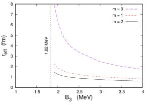
Figure 11: The variation of the effective or mean geometrical matter radius $r_{\rm eff}\equiv\langle r^{2}_{\rm eff}\rangle^{1/2}_{\rm 2n-halo}$ [see Eq. (85)] of the S-wave $D^{0}nn$ $2n$-halo system for various input values of the three-body binding energy $B_{3}$ for the three lowest trimer states ($m=0,1,2$). The vertical dashed line denotes the $D^{0}n+n$ dimer-particle break-up threshold energy $B_{nD}=1.82$ MeV, corresponding to the spin-doublet S-wave scattering length $a_{nD}=4.141$ fm which is extracted in the ZCL scenario Raha:2017ahu .

Finally, we turn to the issue of remnant structural universality, if any, exhibited by the $D^{0}nn$ halo-bound system. We know that on approaching the unitary limit with $a_{nn},a_{nD}\rightarrow\pm\infty$, the square root of the ratio of the relative three-body binding energy $B_{T}$ of two successive Efimov states is expected to approach the universal transcendental number $\lambda^{\infty}_{0}$ characterizing the discrete scaling invariance of the system due to the asymptotic RG limit cycle signature:

$$\sqrt{\frac{B_{3}^{(m)}}{B^{(m+1)}_{3}}}\sim\sqrt{\frac{B_{T}^{(m)}}{B^{(m+1)}_{T}}}\to\lambda^{\infty}_{0}=e^{\pi/s^{\infty}_{0}}=21.5064...\,,$$ (87)

where $B_{T}=B_{3}-B_{nD}\sim B_{3}$, asymptotically, and so do the corresponding successive inverse ratios of the generic rms radii $r\equiv\sqrt{\langle r^{2}\rangle}$, namely,

$$\frac{r^{(m+1)}}{r^{(m)}}\to\lambda^{\infty}_{0}=21.5064...\,.$$ (88)

However, at the physical point of the system (i.e., with finite $a_{nn},\,a_{nD},\Lambda_{\rm reg}<\infty$), only the ratios $\sqrt{B_{T}^{(m)}/B_{T}^{(m+1)}}$ are obtained somewhat close to asymptotic value $\lambda^{\infty}_{0}$, rapidly converging to the same limit as $\Lambda_{\rm reg}\to\infty$. In contrast, the ratios $\sqrt{B_{3}^{(m)}/B_{3}^{(m+1)}}$ are found to differ substantially from the asymptotic scaling factor, especially for small $\Lambda_{\rm reg}$ values, with a rather slow asymptotic convergence. In fact, we find that the convergence pattern exhibited by the successive ratios of the generic rms radii can be much better reconciled with the convergence pattern of the ratios of $1/\sqrt{B_{3}}$ rather than those of $1/\sqrt{B_{T}}$, corroborating with the similar findings of Refs. DL-Canham:2009 ; Canham:2008jd , i.e.,

$$\frac{r^{(m+1)}}{r^{(m)}}\sim\sqrt{\frac{B_{3}^{(m)}}{B_{3}^{(m+1)}}}\nsim\sqrt{\frac{B_{T}^{(m)}}{B_{T}^{(m+1)}}}\,.$$ (89)

To see this numerically, we re-visit our results for the cut-off dependence of the three-body binding energies for the ground ($m=0$) and first two excited ($m=1,2$) states of the $D^{0}nn$ system [cf. Fig. 9, left plot]. For instance, with the choice of the cut-off as $\Lambda_{\rm reg}=1473$ MeV, the binding energy for the shallowest, i.e., the first ($m=1$) excited state is obtained as $B^{(1)}_{3}=1.92$ MeV ($B^{(1)}_{T}=0.1$ MeV), while that of the ground ($m=0$) state is obtained as $B^{(0)}_{3}=76.63$ MeV ($B^{(0)}_{T}=74.81$ MeV). Thus, we can expect the ratios of the rms radii to roughly follow the non-asymptotic correspondence

$$\frac{r^{(1)}}{r^{(0)}}\sim\sqrt{\frac{B_{3}^{(0)}}{B_{3}^{(1)}}}=6.32\,,$$ (90)

in contrast to the ratio $\sqrt{B_{T}^{(0)}/B_{T}^{(1)}}=27.35$ which quickly approaches close to the asymptotic limit $21.5064...$ for larger $\Lambda_{\rm reg}$ values. As displayed in Table 5, the radius ratios are roughly the size of the non-asymptotic values of the 1/$\sqrt{B_{3}}$ ratios, and are expected to follow a similar convergence pattern (although, numerically the radius ratios vary among each other) as $\Lambda_{\rm reg}\to\infty$. In fact, with $\Lambda_{\rm reg}=31467$ MeV, that corresponds to the second ($m=2$) excited state (the shallowest state) with the same binding energy $B^{(2)}_{3}=1.92$ MeV ($B^{(2)}_{T}=0.1$ MeV), the various ratios $r^{(1)}/r^{(0)}$ displayed in the table are seemingly closer to the asymptotic value. Whereas, the corresponding ratios $r^{(2)}/r^{(1)}$ still lag behind exhibiting slower convergence rates. Of course, it should go without mentioning that the ground state at such large cut-offs becomes so anomalously deep that the identification of the $D^{0}nn$ ground state as an Efimov state in low-energy EFT becomes questionable.

RMS Radius	$m^{\rm th}$ level	(1) $r_{nn}$	(2) $r_{nD}$	(3) $r_{n}$	(4)$r_{D}$	(5) $r_{n-nD}$	(6) $r_{D-nn}$	$r_{\rm eff}$
$\Lambda_{\rm reg}=1473$ MeV,	0	0.49	0.48	0.32	0.22	0.43	0.43	0.28
$\sqrt{\frac{B_{3}^{(0)}}{B_{3}^{(1)}}}=6.32$	1	3.49	3.12	3.67	1.39	3.81	2.67	2.23
Radius ratio $\displaystyle{\frac{r^{(1)}}{r^{(0)}}}$	0 & 1	7.12	6.50	11.47	6.32	8.86	6.21	7.96
$\Lambda_{\rm reg}=31467$ MeV,	0	0.02	0.02	0.01	0.01	0.02	0.02	0.01
$\sqrt{\frac{B_{3}^{(0)}}{B_{3}^{(1)}}}=19.88$,	1	0.25	0.28	0.18	0.14	0.24	0.27	0.16
$\sqrt{\frac{B_{3}^{(1)}}{B_{3}^{(2)}}}=6.24$	2	2.27	2.26	2.44	0.94	2.60	1.88	1.53
$1^{\rm st}$ Radius ratio $\displaystyle{\frac{r^{(1)}}{r^{(0)}}}$	0 & 1	12.50	14.00	18.00	14.00	12.00	13.50	16.00
$2^{\rm nd}$ Radius ratio $\displaystyle{\frac{r^{(2)}}{r^{(1)}}}$	1 & 2	9.08	8.07	13.55	6.71	10.83	6.96	9.56

Table 5: Various leading order root mean squared distances and their successive ratios among the ground ($m=0$), first ($m=1$), and second ($m=2$) excited Efimov trimers for a S-wave halo-bound $D^{0}nn$ system. The regulator cut-offs $\Lambda_{\rm reg}$ are chosen such that the shallowest trimer has a fixed binding energy $B^{(m_{\rm max})}_{3}=1.92$ MeV ($B^{(m_{\rm max})}_{T}=0.1$ MeV). The units of the root mean squared distances are in Fermi (fm). The results correspond to two-body inputs in the ZCL scenario Raha:2017ahu .

To determine the renormalized regulator-independent radii for the S-wave $D^{0}nn$ system, it is necessary to introduce LO 3BF terms and fix their couplings $g_{3}=g_{3}(\Lambda_{\rm reg})$ from the RG limit cycle corresponding to the input $B_{3}$. To introduce the 3BF terms, as discussed earlier, we modify the S-wave single-particle exchange interaction kernels, $\mathcal{K}_{(n)}$ and $\mathcal{K}_{(D)}$, into their renormalized counterparts, $\mathbb{K}^{R}_{(n)}$ and $\mathbb{K}^{R}_{(D)}$, respectively [see Eq (61)], for determining the spectator functions $F_{i}$ using the STM3 equations. Furthermore, the three-particle free Green’s functions, $\mathcal{G}_{0}^{(n)}$ and $\mathcal{G}_{0}^{(D)}$, respectively, are required to be modified into their renormalized counterparts, $\mathbb{G}^{(n)R}_{0}$ and $\mathbb{G}^{(D)R}_{0}$ [see Eq. (24)], namely,

$$\mathcal{G}_{0}^{(i)}(p,q;B_{3})\longrightarrow\mathbb{G}^{(i)R}_{0}(p,q;B_{3})=\mathcal{G}_{0}^{(i)}(p,q;B_{3})-2g_{3}/\Lambda_{\rm reg}^{2}\,,$$ (91)

which are used for determining the LO three-particle renormalized S-wave wavefunctions $\Psi^{R}_{n}$ and $\Psi^{R}_{D}$. The corresponding regulator-independent renormalized S-wave radial probability densities $P^{R}_{n}$ and $P^{R}_{D}$ are displayed in the lower panel of Fig. 7. We now use these renormalized wavefunctions along with the STM3 integral equations to determine the renormalized form factors and their rms radii. The residual regulator dependence of the renormalized rms radii is summarized in Fig. 12, as obtained for three ad hoc binding energy inputs, $B_{3}=1.92,2.82$, and $3.82$ MeV. The numerical data points corresponding to each of the six rms distances (i.e., excluding the effective radius $r_{\rm eff}$) are then fitted with a polynomial equation with free parameters ${\mathcal{R}}_{\alpha}$ and ${\mathscr{R}}_{\alpha}$ ($\alpha=1,...,6$) of the form:

$$r_{\alpha}=r_{\alpha}^{(\infty)}\left(1+\frac{\mathcal{R}_{\alpha}}{\Lambda_{\rm reg}}+\frac{\mathscr{R}_{\alpha}}{\Lambda_{\rm reg}^{2}}\right)\,.$$ (92)

Figure 12 demonstrates the residual scale variations of the renormalized rms radii which are all seen to progressively converge as $\Lambda_{\rm reg}\to\infty$, in agreement with renormalization group invariance. These asymptotic values serve as our LO EFT predictions for the renormalized rms distances.

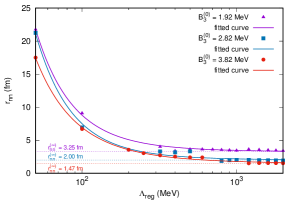
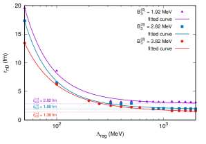
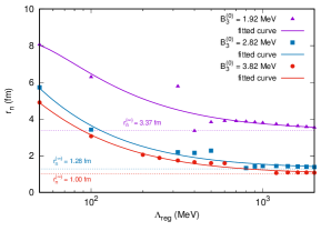
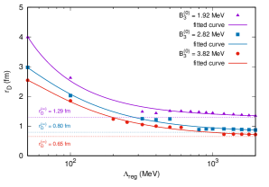
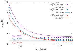
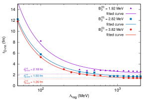
Figure 12: Residual regulator $\Lambda_{\rm reg}$ dependence of the renormalized leading order rms radii of the $D^{0}nn$ ground state for input three-body binding energies $B^{(0)}_{3}=1.92,2.82$, and $3.82$ MeV. In each case, the numerical data points are fitted with a smooth function defined by Eq. (92). The horizontal lines denote the asymptotic values of the respective rms radii $r^{\infty}_{\alpha}$ ($\alpha=1,...6$), as $\Lambda_{\rm reg}\to\infty$. These results correspond to two-body inputs in the ZCL model scenario of Ref. Raha:2017ahu .

In Table. 6 we summarize our LO predictions of the renormalized (asymptotic) radii and the $n-D^{0}-n$ opening angle, corresponding to three distinct ground state binding energies, namely, $B_{3}^{(0)}=1.92,2.82$, and $3.82$ MeV. As expected, we find the three-body system to shrink in size with increasing binding energy. Particularly, in the case of $B_{3}^{(0)}=1.92$ MeV, we already observe $r_{nn}^{(\infty)}$, $r_{n-nD}^{(\infty)}$, and $r_{n}^{(\infty)}$ to supersede $r_{D}^{(\infty)}$ by $\gtrsim 200\%$, and this difference increases progressively further as $B^{(0)}_{3}\to 1.82$ ($B^{(0)}_{T}\to 0$). This evidently indicates the onset that the ground state steadily emerges into a halo-bound universal structure as it is driven close the $D^{0}n+n$ dimer-particle break-up threshold. Figure. 13 illustrates this feature showing the variation of the effective geometrical radius $r_{eff}^{(\infty)}$ with $B_{3}^{(0)}$. The smooth curve shown in the plot is a fit to the data points using a polynomial of the form:

$$B_{3}^{(0)}=1.82\left(1+\frac{\mathcal{B}}{r_{\rm eff}^{(\infty)}}+\frac{\mathscr{B}}{\left(r_{\rm eff}^{(\infty)}\right)^{2}}\right)\,,$$ (93)

where ${\mathcal{B}}$ and ${\mathscr{B}}$ are two fitted parameters.

$B_{3}^{(0)}$ (MeV)	(1) $r_{nn}^{(\infty)}$	(2) $r_{nD}^{(\infty)}$	(3) $r_{n}^{(\infty)}$	(4) $r_{D}^{(\infty)}$	(5) $r_{n-nD}^{(\infty)}$	(6) $r_{D-nn}^{(\infty)}$	$r_{\rm eff}^{(\infty)}$	$\theta^{\infty}_{nn}$
1.92	3.25	2.82	3.37	1.29	3.39	2.18	1.96	73.40
2.82	2.00	1.88	1.28	0.80	1.75	1.50	1.07	67.38
3.82	1.47	1.38	1.00	0.65	1.23	1.26	0.80	60.51

Table 6: Summary of our LO EFT predictions for the renormalized (asymptotic) rms radii $r_{1,...,6}^{(\infty)}$ (in fm), the effective geometrical radius $r_{\rm eff}^{(\infty)}$ (in fm), and the $n-D^{0}-n$ opening angle $\theta^{\infty}_{nn}$ (in degrees), determining the geometrical structure of the S-wave ground state $D^{0}nn$ system. The corresponding input three-body binding energies are $B^{(0)}_{3}=1.92,2.82$, and $3.82$ MeV. These results correspond to two-body inputs in the ZCL model scenario of Ref. Raha:2017ahu .

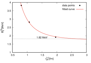
Figure 13: Variation of the effective geometrical radius $r_{eff}^{(\infty)}$ with respect to the ground state binding energy $B_{3}^{(0)}$ of the S-wave $D^{0}nn$ system. The data points correspond to those obtained in Table 6 which are fitted using Eq. 93. The horizontal line depicts the $D^{0}n+n$ dimer-particle break-up threshold energy.

VI Summary and Conclusion

In this work, we have reviewed the effective quantum mechanical formulation of constructing the Faddeev equations in the momentum representation at leading order. Such a formalism was originally developed in Refs. Platter:2004he ; Platter:2004ns ; Platter:2004zs for the investigation of resonant systems of three and four bosons, and was later extended to the study of $2n$-halo nuclei such as the ⁶He, ²⁰C, etc. Canham:2008jd ; DL-Canham:2009 ; Ji:2014wta ; Gobel:2019jba . We subsequently demonstrated the equivalence of the leading order formalism to that of standard leading order pionless/halo-EFT via the STM integral equations STM1 ; STM2 . Next, we used the framework to investigate the universal structural features of the putative S-wave $2n$-halo-bound $D^{0}nn$ system, assuming an idealized ZCL scenario Raha:2017ahu with resonant S-wave interactions between the neutrons and the core $D^{0}$-meson. Using Jacobi coordinate system in momentum representation we constructed a complete set of partial-wave basis states onto which we project the set of coupled integral equations describing the dynamics of the coupled spin and isospin channels for the $D^{0}nn$ system. For such a construction we encountered two essential sets of components, namely, the two-body Lippmann-Schwinger kernels, represented by the form ${}_{i}\langle pq\,\mathcal{Q}_{i}|G_{0}t_{i}|p^{\prime}q^{\prime}\,\mathcal{Q}_{i}\rangle_{i}$, and the re-couplings between the Jacobi representations of different re-arrangement channels, represented by the overlap matrix elements of the form ${}_{i}\langle pq\,\mathcal{Q}_{i}|p^{\prime}q^{\prime}\,\mathcal{Q}_{j}\rangle_{j}$ (where $i,j=n,D$). Especially, in view of the presence of shallow-bound S-wave real-bound bound $D^{0}$-$n$ and virtual-bound $n$-$n$ subsystems, following the approach of Refs Canham:2008jd ; DL-Canham:2009 , it becomes advantageous to use separable S-wave short-distance two-body interactions, thereby allowing us to compute the two-body kernels analytically.

By investigating the asymptotic behavior of the integral equations (without the three-body force terms) an RG limit cycle behavior was revealed with an inherent discrete scaling symmetry characterized by the universal transcendental number $\lambda_{0}^{\infty}=21.5064...$. This is formally indicative of the manifestation of Efimov states below the $D^{0}n+n$ dimer-particle break-up threshold energy $B_{nD}=1.82$ MeV. In particular, by introducing a sharp momentum cut-off in the STM equations and fixing a near-threshold value of the three-body binding energy for the shallowest (most excited) Efimov level, e.g., $B_{T}=B_{3}-B_{nD}=0.1$ MeV, level energies $B_{T}\approx 73$ MeV and $B_{T}\approx 29934$ MeV are yielded as predictions for the two deepest states (although the relevance of such large binding energies lies certainly beyond the realm of the low-energy EFT).

Next, we investigated the remnant structural universality features of the halo-bound $D^{0}nn$ system. For this purpose, we reconstructed the full momentum space leading order S-wave three-body wavefunctions $\Psi_{n}(p,q)$, Eq. (74), and $\Psi_{D}(p,q)$, Eq. (LABEL:eq:Psi_D_pq), following the methodology outlined in Refs. Canham:2008jd ; DL-Canham:2009 . The wavefunctions so constructed were then used to determine the leading order one- and two-body matter density form factors for the ground and the first two excited Efimov states, and hence, extract the corresponding rms radii characterizing the halo-bound structure of the $D^{0}nn$ system. The latter results were also used to determine the two-neutron opening angle $\theta_{nn}$ and the effective geometrical matter radius $r_{\rm eff}$ for the three-body system. In particular, without including the 3BF the unrenormalized results exhibit strong regulator $\Lambda_{\rm reg}$ dependence. Our findings in Table 4 reveal that the rms radii especially the ground state are substantially more sensitive to the regulator variations than the excites states, and tend to become quite large on approaching close to the threshold as $B^{(0)}_{T}\to 0$. This already hints at a halo-like signature for the ground state. The regulator sensitivity, however, diminishes sharply for the excited states which are seemingly more structurally compact. Moreover, the marginal variation of $\theta_{nn}$ for the ground state as compared to the excited states indicates that the strongly attractive $n$-$n$ interaction favors a shallow ground state with a near-equilateral three-particle configuration. Finally, in our quest for a possible signature of remnant structural universality, we indeed observed that the ratios of the rms distances of the successive level states are commensurate with the corresponding ratios of the inverse square root of three-body binding energies $B_{3}$ (as compared to $B_{T}$), namely, $r^{(m+1)}/r^{(m)}\sim\sqrt{B_{3}^{(m)}/B_{3}^{(m+1)}}$. However, at small $\Lambda_{\rm reg}$ values these ratios differ significantly from the asymptotic value characterized by the limit cycle parameter $\lambda_{0}^{\infty}$. Only for sufficiently large $\Lambda_{\rm reg}$, do these ratios approach this limit. However, given that the ground state simultaneously becomes unphysically deep, its practical implication becomes irrelevant in the low-energy EFT picture.

Finally, by including the 3BF terms in the STM3 equations which determine the spectator functions $F_{n,D}$, as well as in the wavefunctions $\Psi_{n,D}$ which determine the form factors, yields our renormalized leading order observables pertaining to the ground state Efimov trimer, as displayed in Table 6. Given the current unavailability of any three-body datum on the $D^{0}nn$ system, several ah hoc input values of the three-body binding energies, namely, $B^{(0)}_{3}=1.92,2.82$, and $3.82$ MeV, were used to obtain our results. As with the two-body inputs, we used the information on the phenomenologically extracted S-wave spin-singlet $nn$ S-wave scattering length, $a_{nn}=-18.63$ fm Chen:2008zzj , as well as the S-wave spin-doublet $nD^{0}$ S-wave scattering length, $a_{nD}=4.141$ fm, with the latter value obtained from the ZCL model analysis of Ref. Raha:2017ahu . As seen in Fig. 12, the results do exhibit residual scale dependence due to lack of renormalizability at small regulator cut-offs. Nevertheless, asymptotic convergence is rapidly achieved beyond $\Lambda_{\rm reg}\gtrsim 450-500$ MeV. With the leading order results converging at scales not too large in comparison to the pion mass, the hard scale of ${}^{\pi\!\!\!\!/}$EFT, evokes encouraging prospects of realizing the $2n$-halo $D^{0}nn$ system as either a realistic Efimov ground state or a quasi-bound Efimov resonance. Moreover, given that a leading order EFT analysis is primarily qualitative, it certainly leaves room for more a robust treatment by systematically including next-to-leading order corrections. However, the major drawback in this regard is that the poorly constrained $DN$ interactions make the extraction of the S-wave parameters, e.g., the $D^{0}n$ effective range, currently unpracticable.

In conclusion, more investigations on the $D^{0}nn$ three-body system, particularly on the experimental front, are needed to throw light on the possible existence of an Efimov bound or quasi-bound resonance state. Due to the current paucity of phenomenological information, as well as the complications of including decay and coupled-channel dynamics which tend to dis-favor universality, it is quite a challenging task to theoretically extract the remnant Efimovian signatures reliably. It is far more conceivable, nonetheless, that near-future experiments at facilities like J-PARC, KEK, and FAIR, might be able to probe specific signatures of the haloing/clustering dynamics manifested in the $D^{0}nn$ system.

Appendix A Basis states in Jacobi momentum representation

The Jacobi momenta provide a convenient representation to describe the non-relativistic dynamics of a three-body system. By completely eliminating the motion of the center-of-mass of the three-body system, it expresses all the dynamics in terms of the binary subsystem’s internal relative motion, as well as the motion of the binary subsystem relative to the spectator particle. Thus, the momentum state of an arbitrary three-body system is defined in terms of a pair of relative three-momenta: one being the relative three-momentum ${\bf p}$ between two particles in a chosen two-body subsystem, and the other being the three-momentum ${\bf q}$ of the third spectator particle relative to the center-of-mass of the chosen binary subsystem.

For concreteness, as depicted in Fig. 14, let us consider an arbitrary system of three distinguishable particles $i,j$ and $k$ with masses $m_{i}$, $m_{j}$ and $m_{k}$, and the individual laboratory/inertial frame momentum ${\bf k}_{i}$, ${\bf k}_{j}$ and ${\bf k}_{k}$, respectively. Then, the Jacobi momenta of the system with particle $i$ as the spectator are defined by

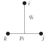
Figure 14: The Jacobi momenta ($p_{i}=|{\bf p}_{i}|,q_{i}=|{\bf q}_{i}|$) for an arbitrary three-body system.

$${\bf p}_{i} = \mu_{jk}\left(\frac{{\bf k}_{j}}{m_{j}}-\frac{{\bf k}_{k}}{m_{k}}\right)\,;\qquad\mu_{jk}=\frac{m_{j}m_{k}}{m_{j}+m_{k}}\,,$$ (94)

$${\bf q}_{i} = \mu_{i(jk)}\left(\frac{{\bf k}_{i}}{m_{i}}-\frac{{\bf k}_{j}+{\bf k}_{k}}{m_{j}+m_{k}}\right)\,;\qquad\mu_{i(jk)}=\frac{m_{i}(m_{j}+m_{k})}{M}\,.$$ (95)

Here, ${\bf p}_{i}$ is the relative momentum between the particles $j$ and $k$ in the center-of-mass frame of the two-body subsystem, ${\bf q}_{i}$ is the relative momentum of the spectator particle $i$ with respect to the center-of-mass of the same binary subsystem, $M=m_{i}+m_{j}+m_{k}$ is the total mass of the three-body system, and ${\bf K}={\bf k}_{i}+{\bf k}_{j}+{\bf k}_{k}$ is total three-body momentum. With the above choice of the Jacobi momenta, the total kinetic energy or free Hamiltonian of the three-body system is given as

$$H_{0}=\frac{{\bf K}^{2}}{2M}+\frac{{\bf p}^{2}_{i}}{2\mu_{jk}}+\frac{{\bf q}^{2}_{i}}{2\mu_{i(jk)}}\,.$$ (96)

A.1 Jacobi momentum basis in quantum mechanics

We now briefly discuss the construction of a complete set of basis states for a momentum-space quantum mechanical description of an arbitrary three-body system. For a detailed exposition, we refer the reader to Ref. Glockle_1983 . The basic objects are the Jacobi plane wave state vectors denoted as

$$|{\bf p},{\bf q}\rangle_{i}\equiv|{\bf p}_{i},{\bf q}_{i}\rangle_{i}\,,$$ (97)

which satisfy the orthonormality relation:

$${}_{i}\langle{\bf p},{\bf q}|{\bf p}^{\prime},{\bf q}^{\prime}\rangle_{i}\equiv{}_{i}\langle{\bf p}_{i},{\bf q}_{i}|{\bf p}^{\prime}_{i},{\bf q}^{\prime}_{i}\rangle_{i}=\delta^{3}({\bf p}_{i}-{\bf p}^{\prime}_{i})\,\delta^{3}({\bf q}_{i}-{\bf q}^{\prime}_{i})\equiv\delta^{3}({\bf p}-{\bf p}^{\prime})\,\delta^{3}({\bf q}-{\bf q}^{\prime})\,,$$ (98)

as well as the completeness relation:

$$\int{\rm d}^{3}{\bf p}\int{\rm d}^{3}{\bf q}\,|{\bf p},{\bf q}\rangle_{i}\,\,{}_{i}\langle{\bf p},{\bf q}|\equiv\int{\rm d}^{3}{\bf p}_{i}\int{\rm d}^{3}{\bf q}_{i}\,|{\bf p}_{i},{\bf q}_{i}\rangle_{i}\,\,{}_{i}\langle{\bf p}_{i},{\bf q}_{i}|=\mathbb{I}\,.$$ (99)

Since these momentum states denote free-particle motions, they are eigenstates of the free Hamiltonian $H_{0}$:

$$H_{0}|{\bf p}_{i},{\bf q}_{i}\rangle=\left(\frac{{\bf p}^{2}_{i}}{2\mu_{jk}}+\frac{{\bf q}^{2}_{i}}{2\mu_{i(jk)}}\right)|{\bf p}_{i},{\bf q}_{i}\rangle$$ (100)

A generic partial wave projected basis can now be constructed from the above plane wave states Glockle_1983 :

$$|pq\,\mathcal{Q}_{i}\rangle_{i}\equiv\Big{|}pq\big{\{}(l,s)\mathcal{j},(\lambda,\sigma)\mathcal{J}\big{\}}JM_{J},(t,\tau)TM_{T}\Big{\rangle}_{i}\,,$$ (101)

where $\mathcal{Q}_{i}$ specifies the set of all spin and isospin quantum numbers for a given quantum state, defined with respect to the particle $i$ as the spectator. For the above basis representation $\mathcal{Q}_{i}$ collectively denotes the following spin-isospin quantum numbers:

• $l\implies$ quantum number for the relative orbital angular momentum of particles in binary subsystem $j$-$k$,

• $s\implies$ intrinsic spin quantum number of binary subsystem $j$-$k$,

• $\mathcal{j}=l\oplus s\implies$ total spin quantum number of binary subsystem $j$-$k$,

• $t\implies$ isospin quantum number of binary subsystem $j$-$k$,

• $\lambda\equiv l_{i}\implies$ orbital angular momentum quantum number of spectator $i$ relative to binary subsystem $j$-$k$,

• $\sigma\equiv s_{i}\implies$ intrinsic spin quantum number of spectator $i$,

• $\mathcal{J}=\lambda\oplus\sigma\implies$ total spin quantum number of spectator $i$,

• $\tau\equiv t_{i}\implies$ isospin quantum numbers of spectator $i$,

• $J=\mathcal{j}\oplus\mathcal{J}\implies$ total spin quantum number of three-body system,

• $M_{J}\implies$ quantum number for the $z$-component of total spin of three-body system,

• $T=t\oplus\tau\implies$ total isospin quantum number of three-body system,

• $M_{T}\implies$ quantum number for the $z$-component of total isospin of three-body system.

However, it is sometimes useful to re-couple the orbital angular momentum, intrinsic spin, and isospin quantum numbers of the full three-body system, instead of using the aforementioned representation in terms of the (2+1)-subsystem quantum numbers. This amounts to an unitary transformation of the $|pq\,\mathcal{Q}\rangle_{i}$ basis which is easily achieved via the Wigner’s 9-j symbol:

$$|pq\,\mathcal{Q}_{i}\rangle_{i}=\sum_{LS}\sqrt{\hat{\mathcal{j}}\,\hat{\mathcal{J}}\,\hat{L}\,\hat{S}}\begin{Bmatrix}l&s&\mathcal{j}\\ \lambda&\sigma&\mathcal{J}\\ L&S&J\\ \end{Bmatrix}\Big{|}pq\big{\{}(l,\lambda)L,(s,\sigma)S\big{\}}JM_{J},(t,\tau)TM_{T}\Big{\rangle}_{i}\,,$$ (102)

where it is customary to denote the hatted quantum numbers, e.g., $\hat{\mathcal{j}}\equiv 2\mathcal{j}+1$, etc. Also,

• $L=l\oplus\lambda\implies$ total orbital quantum number of three-body system,

• $S=s\oplus\sigma\implies$ total intrinsic spin quantum number of three-body system.

These partial-wave-projected basis state vectors likewise satisfy the orthonormality relation:

$${}_{i}\langle pq\,\mathcal{Q}_{i}|p^{\prime}q^{\prime}\,\mathcal{Q}_{i}\rangle_{i}=\frac{\delta(p-p^{\prime})}{pp^{\prime}}\frac{\delta(q-q^{\prime})}{qq^{\prime}}\,,$$ (103)

as well as the completeness relation:

$$\sum_{\mathcal{Q}_{i}}\int_{0}^{\infty}{\rm d}p\,\,p^{2}\int_{0}^{\infty}{\rm d}q\,\,q^{2}\,\,|pq\,\mathcal{Q}_{i}\rangle_{i}\,\,{}_{i}\langle pq\,\mathcal{Q}_{i}|=\mathbb{I}\,,$$ (104)

such that a Faddeev component $|\psi_{i}\rangle$ may be expanded in the basis as follows:

$$|\psi_{i}\rangle=\sum_{\mathcal{Q}_{i}}\int_{0}^{\infty}{\rm d}p\,\,p^{2}\int_{0}^{\infty}{\rm d}q\,\,q^{2}\,\,{}_{i}\langle pq\,\mathcal{Q}_{i}|\psi_{i}\rangle\,\,|pq\,\mathcal{Q}_{i}\rangle_{i}\,.$$ (105)

Here we also display how we express the overlap of a plane wave vector state onto a partial wave projected state employing spherical and hyperspherical harmonics, namely,

$${}_{i}\langle{\bf p}^{\prime}|plm_{l}\rangle_{i} = \frac{\delta(p-p^{\prime})}{pp^{\prime}}Y^{m_{l}}_{l}(\hat{\bf p}^{\prime})\,,$$ (106)

$${}_{i}\langle{\bf p}^{\prime},{\bf q}^{\prime}|pq(l\lambda)LM_{L}\rangle_{i} = \frac{\delta(p-p^{\prime})}{pp^{\prime}}\frac{\delta(q-q^{\prime})}{qq^{\prime}}\mathcal{Y}_{l\lambda}^{LM_{L}}(\hat{\bf p}^{\prime},\hat{\bf q}^{\prime})\,.$$ (107)

The solutions to the Faddeev equations will also require us to re-couple two Jacobi basis states corresponding to different spectator representations. This corresponds to the overlap matrix element of the form:

$${}_{i}\langle pq\,\mathcal{Q}_{i}|p^{\prime}q^{\prime}\,\mathcal{Q}_{j}\rangle_{j} = \sum_{LS}\sum_{L^{\prime}S^{\prime}}\sqrt{\hat{\mathcal{j}}\hat{\mathcal{J}}\hat{L}\hat{S}}\sqrt{\hat{\mathcal{j}^{\prime}}\hat{\mathcal{J}^{\prime}}\hat{L^{\prime}}\hat{S^{\prime}}}\begin{Bmatrix}l&s&\mathcal{j}\\ \lambda&\sigma&\mathcal{J}\\ L&S&J\\ \end{Bmatrix}\begin{Bmatrix}l^{\prime}&s^{\prime}&\mathcal{j}^{\prime}\\ \lambda^{\prime}&\sigma^{\prime}&\mathcal{J}^{\prime}\\ L^{\prime}&S^{\prime}&J^{\prime}\\ \end{Bmatrix}$$ (108)

$$\times{}_{i}\langle pq(l\lambda)L|p^{\prime}q^{\prime}(l^{\prime}\lambda^{\prime})L^{\prime}\rangle_{j}\,\,\,{}_{i}\langle(s\sigma)S|(s^{\prime}\sigma^{\prime})S^{\prime}\rangle_{j}\,\,\,{}_{i}\langle(t\tau)T|(t^{\prime}\tau^{\prime})T^{\prime}\rangle_{j}\,,\quad\,$$

where the re-coupling matrix elements for the spins and isospins are calculated using the Wigner’s 6-j symbol:

$${}_{i}\langle(s\sigma)S|(s^{\prime}\sigma^{\prime})S^{\prime}\rangle_{j}=\delta_{SS^{\prime}}\sqrt{\hat{s}\hat{s}^{\prime}}(-1)^{s_{i}+s_{j}+s_{k}+S}\begin{Bmatrix}s_{j}&s_{k}&s\\ s_{i}&S&s^{\prime}\\ \end{Bmatrix}\,,$$ (109)

and

$${}_{i}\langle(t\tau)T|(t^{\prime}\tau^{\prime})T^{\prime}\rangle_{j}=\delta_{TT^{\prime}}\sqrt{\hat{t}\hat{t}^{\prime}}(-1)^{t_{i}+t_{j}+t_{k}+T}\begin{Bmatrix}t_{j}&t_{k}&t\\ t_{i}&T&t^{\prime}\\ \end{Bmatrix}\,.$$ (110)

The overlap matrix elements ${}_{i}\langle pq(l\lambda)L|p^{\prime}q^{\prime}(l^{\prime}\lambda^{\prime})L^{\prime}\rangle_{j}$ involve re-couplings between momenta and orbital angular momenta belonging to different spectator representations. The general procedure of evaluating such matrix elements is somewhat elaborate but well-known in the literature Glockle_1983 ; Canham:2008jd ; DL-Canham:2009 ; Platter:2004he ; Platter:2004ns ; Platter:2004zs . Thus, we do not intend to repeat the derivations here. For our case of the $D^{0}nn$ system, the analytical results for the appropriate matrix elements are displayed in the main text in Sec. III.

A.2 Jacobi momenta for the $D^{0}nn$ system

The three different re-arrangement channels for the $D^{0}nn$ system are displayed in Fig.15. For the simplicity of analytical derivations, we find it convenient to express the mass $M_{D}$ of the $D^{0}$-meson in terms of the nucleon (neutron) mass, namely, $M_{D}=yM_{n}$. Also, in order to distinguish between the momenta of the two identical neutrons, we find it convenient to tag them as $n_{1}$-neutron and $n_{2}$-neutron. Quantum mechanically, however, anti-symmetry is demanded to preserve the parity of the wavefunctions under permutations. Depending on the choice of the spectator, the following equivalent kinematical description of the $D^{0}nn$ system can be given:

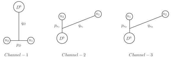
Figure 15: The re-arrangement channels and Jacobi momenta for the $D^{0}nn$ system.

• Channel-1: $D^{0}$-meson is the spectator, and the two neutrons form the binary subsystem. In this case, the choice of the Jacobi momenta are

  $${\bf p}_{D}=\frac{1}{2}({\bf k}_{n_{1}}-{\bf k}_{n_{2}})\,,\qquad\text{and}\qquad{\bf q}_{D}=\frac{2{\bf k}_{D}-y({\bf k}_{n_{1}}+{\bf k}_{n_{2}})}{y+2}\,,$$ (111)

  where ${\bf k}_{n_{1}}$, ${\bf k}_{n_{2}}$, and ${\bf k}_{D}$ are individual momenta of $n_{1}$-neutron, $n_{2}$-neutron and the $D^{0}$-meson, respectively. The corresponding free Hamiltonian of the system in this representation is given by

  $$H_{0}^{(D)}=\frac{{\bf p}_{D}^{2}}{2\mu_{nn}}+\frac{{\bf q}_{D}^{2}}{2\mu_{D(nn)}}=\frac{1}{M_{n}}p_{D}^{2}+\left(\frac{y+2}{4yM_{n}}\right)q_{D}^{2}\,,$$ (112)

  where the reduced masses are defined as

  $$\mu_{nn}=\frac{M_{n}}{2}\quad\text{and}\quad\mu_{D(nn)}=\frac{2M_{n}M_{D}}{M_{D}+2M_{n}}=\frac{2y}{y+2}M_{n}\,.$$ (113)

• Channels-2, -3: Either $n_{1}$-neutron or $n_{2}$-neutron is the spectator, while the non-spectator neutron with the $D^{0}$-meson forms the binary subsystem. These two re-arrangement channels yield identical configurations since the two neutrons are identical particles. As noted earlier, using the permutation operator $\mathcal{P}$ the $|\psi_{n2}\rangle$ component wavefunction is expressible in term of the $|\psi_{n1}\rangle$ Faddeev component. In this case, the choice of the Jacobi momenta are

  $${\bf p}_{n_{1}}=\frac{1}{y+1}\left(y{\bf k}_{n_{2}}-{\bf k}_{D}\right)\,,\quad{\bf p}_{n_{2}}=\frac{1}{y+1}\left({\bf k}_{D}-y{\bf k}_{n_{1}}\right)\,,\qquad\text{and}$$

  $${\bf q}_{n_{1}}=\frac{(y+1){\bf k}_{n_{1}}-({\bf k}_{n_{2}}+{\bf k}_{D})}{y+2}\,,\quad{\bf q}_{n_{2}}=\frac{(y+1){\bf k}_{n_{2}}-({\bf k}_{n_{1}}+{\bf k}_{D})}{y+2}\,.$$ (114)

  The corresponding free Hamiltonian is

  $$H_{0}^{(n)}=\frac{{\bf p}_{n}^{2}}{2\mu_{nD}}+\frac{{\bf q}_{n}^{2}}{2\mu_{n(nD)}}=\frac{y+1}{2yM_{n}}p_{n}^{2}+\left(\frac{y+2}{2M_{n}(y+1)}\right)q_{n}^{2}\,,$$ (115)

  where the reduced masses are defined as

  $$\mu_{nD}=\frac{M_{n}M_{D}}{M_{D}+M_{n}}=\frac{y}{y+1}M_{n},\quad\text{and}\quad\mu_{n(nD)}=\frac{M_{n}(M_{D}+M_{n})}{M_{D}+2M_{n}}=\frac{y+1}{y+2}M_{n}\,.$$ (116)

Appendix B Two-body T-matrix with a separable potential

Here we review the quantum mechanical framework, developed originally in the Refs. Platter:2004he ; Platter:2004ns ; Platter:2004zs ; DL-Canham:2009 , and subsequently used in the study of two-body S-wave bound states for a single-channel (rank 1) attractive local potential which is separable. In the momentum space such a model potential can be represented as

$$\frac{1}{(2\pi)^{3}}\langle{\bf k}^{\prime}|V^{S}|{\bf k}\rangle=V({\bf k},{\bf k^{\prime}})=C_{0}\chi(k)\chi(k^{\prime})+\cdots\,,$$ (117)

where $C_{0}<0$ is a two-body coupling constant, and the ellipses denote contributions from higher partial waves that do not concern us. The separable potential can also be expressed in the form of a projection operator:

$$V^{S}\equiv C_{0}|\chi\rangle\langle\chi|\,,$$ (118)

where $\chi(p)=\langle{\bf p}|\chi\rangle$ and $\chi(p^{\prime})=\langle\chi|{\bf p^{\prime}}\rangle$ are the so-called form factor functions. Here we consider their choice for the $l^{\rm th}$ partial wave proportional to the Heaviside step function of the form:

$$\chi_{l}(k,\beta_{l})=k^{l}\Theta(\beta_{l}-k)\,,$$ (119)

where the prefactor $k^{l}$ constrains the T-matrices to satisfy the well-known Wigner threshold law Wigner:1948zz . In our treatment, however, we only consider S-wave ($l=0$) case, for which we have $\chi_{0}\equiv\chi$ with $\beta_{0}\equiv\Lambda_{\rm reg}$. Such regulator functions are used to suppress dynamical contributions arising from the high-momentum region, i.e., for $k,k^{\prime}\geq\beta_{l}$, where $\beta_{l}$’s are cut-off parameters defining the effective range of the potential. In other words, taking $\beta_{l}\to\infty$ is equivalent to considering a zero-range potential.

Now, it is easy to show that for a separable potential $V^{S}$ the two-body T-matrix is itself separable. To this end we consider the T-matrix given by the Lippmann-Schwinger equation in the operator form:

$$t(z)=V^{S}+V^{S}g_{0}(z)t(z)=C_{0}|\chi\rangle\langle\chi|+C_{0}|\chi\rangle\langle\chi|g_{0}(z)t(z)\,.$$ (120)

Multiplying by $\langle\chi|g_{0}$ from the left, we have

$$\langle\chi|g_{0}(z)t(z)=C_{0}\langle\chi|g_{0}(z)|\chi\rangle\langle\chi|+C_{0}\langle\chi|g_{0}(z)|\chi\rangle\langle\chi|g_{0}(z)t(z)\,.$$ (121)

Solving for $\langle\chi|g_{0}t$ we get,

$$\langle\chi|g_{0}(z)t(z)=\frac{\langle\chi|g_{0}(z)|\chi\rangle\langle\chi|}{C^{-1}_{0}-\langle\chi|g_{0}(z)|\chi\rangle}\,.$$ (122)

On inserting it back into the T-matrix equation, we obtain the separable form:

$$t(z)=C_{0}|\chi\rangle\langle\chi|+\frac{C_{0}|\chi\rangle\langle\chi|g_{0}(z)|\chi\rangle\langle\chi|}{C^{-1}_{0}-\langle\chi|g_{0}(z)|\chi\rangle}\equiv|\chi\rangle\tau(z)\langle\chi|\,,$$ (123)

where

$$\tau(z)=\frac{1}{C^{-1}_{0}-\langle\chi|g_{0}(z)|\chi\rangle}\,.$$ (124)

Next, let us express the S-wave T-matrix $T({\bf k},{\bf k^{\prime}};{\mathcal{E}})\equiv-\langle{\bf k}^{\prime}|t|{\bf k}\rangle/(2\pi)^{3}$ via the Lippmann-Schwinger equation in the momentum representation:

$$T({\bf k},{\bf k^{\prime}};{\mathcal{E}}) = V({\bf k},{\bf k^{\prime}})+\int{\rm d}^{3}{\bf p}\,\frac{V({\bf k},{\bf p})}{{\mathcal{E}}-\frac{p^{2}}{2\mu}+i\varepsilon}T({\bf p},{\bf k^{\prime}};{\mathcal{E}})$$ (125)

$$= C_{0}\chi(k,\Lambda_{\rm reg})\,\chi(k^{\prime},\Lambda_{\rm reg})+C_{0}\chi(k,\Lambda_{\rm reg})\int{\rm d}^{3}{\bf p}\,\frac{\chi(p,\Lambda_{\rm reg})}{{\mathcal{E}}-\frac{p^{2}}{2\mu}+i\varepsilon}T({\bf p},{\bf k^{\prime}};{\mathcal{E}})$$

$$= C_{0}\chi(k,\Lambda_{\rm reg})\,\chi(k^{\prime},\Lambda_{\rm reg})\bigg{[}1+C_{0}{\mathcal{I}}({\mathcal{E}},\Lambda_{\rm reg})+C_{0}^{2}{\mathcal{I}}^{2}({\mathcal{E}},\Lambda_{\rm reg})+\cdots\bigg{]}$$

$$\equiv \chi(k,\Lambda_{\rm reg})\,\chi(k^{\prime},\Lambda_{\rm reg})\frac{1}{C^{-1}_{0}-{\mathcal{I}}({\mathcal{E}},\Lambda_{\rm reg})}\,,$$

where

$${\mathcal{I}}({\mathcal{E}},\Lambda_{\rm reg}) = \int{\rm d}^{3}{\bf p}\,\frac{|\chi(p,\Lambda_{\rm reg})|^{2}}{{\mathcal{E}}-\frac{p^{2}}{2\mu}+i\varepsilon}=8\pi\mu\int_{0}^{\infty}{\rm d}p\,p^{2}\frac{\Theta^{2}(\Lambda_{\rm reg}-p)}{2\mu{\mathcal{E}}-p^{2}+i\varepsilon}$$ (126)

$$= 8\pi\mu\int_{0}^{\infty}{\rm d}p\,p^{2}\frac{\Theta(\Lambda_{\rm reg}-p)}{2\mu{\mathcal{E}}-p^{2}+i\varepsilon}=8\pi\mu\int_{0}^{\Lambda_{\rm reg}}{\rm d}p\,p^{2}\frac{1}{2\mu{\mathcal{E}}-p^{2}+i\varepsilon}\,,$$

Since we are concerned with two-body bound states where the total energy is negative (${\mathcal{E}}<0$), the $i\varepsilon$ prescription in the denominator of integral $\mathcal{I}$ becomes redundant. A straightforward evaluation of the integration leads to the following closed-form expression:

$${\mathcal{I}}({\mathcal{E}},\Lambda_{\rm reg})=-4\pi^{2}\mu\bigg{[}\frac{2}{\pi}\Lambda_{\rm reg}-\sqrt{-2\mu{\mathcal{E}}}\,\frac{2}{\pi}\arctan\bigg{(}\frac{\Lambda_{\rm reg}}{\sqrt{-2\mu{\mathcal{E}}}}\bigg{)}\bigg{]}\,.$$ (127)

Taking the zero-range limit, i.e., $\Lambda_{\rm reg}\rightarrow\infty$, the first term in the above expression yields an ultraviolet divergence. Since low-energy observables are expected to be independent of regulators, such terms are eliminated through proper renormalization prescription. With the binary S-wave system with large positive (negative) scattering length $a_{0}$ a two-body shallow bound (virtual) state with energy ${\mathcal{E}}=-B_{2}=-1/(2\mu a^{2}_{0})$ is produced at leading order. This is indicated by the pole position of the two-body T-matrix, represented by the condition:

$$\frac{1}{C_{0}}={\mathcal{I}}({\mathcal{E}}=-B_{2},\Lambda_{\rm reg})\,.$$ (128)

Utilizing the pole position we can now fix the running of the two-body coupling $C_{0}\to C_{0}(\Lambda_{\rm reg})$ in order to reproduce the scattering length $a_{0}$. In particular with $a_{0}\Lambda_{\rm reg}>>1$ leads to a simpler expression:

$$C_{0}(\Lambda_{\rm reg})=\frac{a_{0}}{4\pi^{2}\mu}\bigg{[}1-\frac{2a_{0}\Lambda_{\rm reg}}{{\pi}}\bigg{]}^{-1}\,.$$ (129)

Thus, the renormalized two-body T-matrix for negative energies (${\mathcal{E}}<0$) in the vicinity of an S-wave bound/anti-bound state at the leading order is given by

$$T({\bf k},{\bf k^{\prime}};{\mathcal{E}}) = \chi(k,\Lambda_{\rm reg})\,\chi(k^{\prime},\Lambda_{\rm reg})\frac{1}{4\pi^{2}\mu}\bigg{[}\frac{1}{a_{0}}\,\frac{2}{\pi}\arctan\big{(}|a_{0}|{\Lambda_{\rm reg}}\big{)}$$ (130)

$$\hskip 136.5733pt-\,\sqrt{-2\mu{\mathcal{E}}}\,\frac{2}{\pi}\arctan\bigg{(}\frac{\Lambda_{\rm reg}}{\sqrt{-2\mu{\mathcal{E}}}}\bigg{)}\bigg{]}^{-1}\,.$$

Appendix C Numerical implementation

Finally, we elaborate on our numerical procedure for solving the coupled system of Faddeev integral equations for the $D^{0}nn$ system, Eq. (46), namely,

$$F_{n} = \mathcal{K}_{nn}F_{n}+\mathcal{K}_{nD}F_{D}\,,$$

$$F_{D} = \mathcal{K}_{Dn}F_{n}\,.$$ (131)

The coupled-channel equations could be reduced to a single algebraic equation with two unknown quantities $F_{n}$ and $F_{D}$ which must be solved. Hence, the system of equations does not yield unique solutions. In order to facilitate a solution, we assume the particular form of the solutions, namely, $F_{n}=1$ and $F_{D}=\mathcal{K}_{Dn}F_{n}$.

Since we perform the numerical integrations using Gaussian quadratures, the integration measure ${\rm d}q^{\prime}$ is replaced by a summation over $N$ Gaussian weights $w_{i}$, with $q=q_{i}$ and $q^{\prime}=q^{\prime}_{j}$ being the discrete Gaussian points between 0 and the ultraviolet cut-off momentum $\Lambda_{\rm reg}$. With the numerical integration defined over $N$ Gaussian quadrature points, the spectator function $F_{n}=F_{n}(q^{\prime})$ becomes a $N$-dimensional array with all elements equal to 1, while the kernel function $\mathcal{K}_{Dn}=\mathcal{K}_{Dn}(q,q^{\prime})$ [cf. Eq. (III.4)] becomes an $N\times N$-dimensional matrix defined over the mesh points $(q_{i},q^{\prime}_{j})$, namely,

$$\mathcal{K}_{Dn}(q_{i},q^{\prime}_{j}) = -\frac{2(y+1)}{\pi y}W_{j}q^{\prime\,2}_{j}\mathcal{K}_{(n)}(q_{j}^{\prime},q_{i};B_{3})\,S^{R}_{d}\left(-B_{3}-\frac{q^{\prime 2}_{j}}{2M_{n}},{\bf q}^{\prime}_{j}\right)\,,$$ (132)

where $W_{j}=W(q^{\prime}_{j})$ is the weight factor associated with a given quadrature point $q^{\prime}_{j}$. Finally, the matrix multiplication of $\mathcal{K}_{Dn}$ with the vector $F_{n}$ yields $F_{D}$ as an $N$-dimensional vector:

$$F_{D}(q_{i})=\sum_{j=1}^{N}\mathcal{K}_{Dn}(q_{i},q^{\prime}_{j})\,F_{n}(q^{\prime}_{j})\,.$$ (133)

Furthermore, for the purpose of evaluating the three-body wavefunctions, Eqs. (74) and (LABEL:eq:Psi_D_pq), it is required that the solutions to the spectator functions $F_{n}$ and $F_{D}$ be evaluated at shifted values of the off-shell relative momentum $q^{\prime}=\Pi^{\prime}$ [see Eqs. (72), (73), and (77)]. For this purpose, we use interpolated values of these functions which are easily obtained via a cubic spline interpolation algorithm of the form:

$$F_{i}(\Pi^{\prime})\approx\sum_{j}{\mathcal{S}}_{j}(\Pi^{\prime})F_{i}(q^{\prime}_{j})\,;\quad i=n,D\,,$$ (134)

where ${\mathcal{S}}_{j}$ are the spline elements evaluated at the desired momentum $q^{\prime}=\Pi^{\prime}$. Likewise, the spline interpolator is needed for evaluating the matter density from factors at the shifted values of the momentum transfer $p\to|{\bf p}-{\bf k}|$ or $q\to|{\bf q}-{\bf k}|$, [see Eqs. (79) and (82)].

References

- (1) V. Efimov, “Energy levels arising from the resonant two-body forces in a three-body system”, Phys. Lett. B 33, 563 (1970).
- (2) V. N. Efimov, “Weakly-bound states of 3 resonantly-interacting particle”,, Yad. Fiz. 12, 1080 (1970) [Sov. J. Nucl. Phys. 12, 589 (1971)].
- (3) V. Efimov, “Energy levels of three resonantly interacting particles”, Nucl. Phys. A 210, 157 (1973).
- (4) G. S. Danilov, ”On the three-body problem with short-range forces”, Zh. Eksp. Teor. Fiz. 40, 498 (1961) [Sov. Phys. JETP 13, 349 (1961)].
- (5) L. D. Faddeev, “Scattering theory for a three-particle system”, Sov. Phys. JETP 12, 1014 (1961) [Zh. Eksp. Teor. Fiz 39, 1459 (1960)].
- (6) E. Braaten and H. W. Hammer, “Universality in few-body systems with large scattering length”, Phys. Rept. 428, 259-390 (2006).
- (7) P. Naidon and S. Endo, “Efimov Physics: a review”, Rept. Prog. Phys. 80, no.5, 056001 (2017).
- (8) D. B. Kaplan, M. J. Savage and M. B. Wise, “Nucleon - nucleon scattering from effective field theory”, Nucl. Phys. B 478, 629 (1996).
- (9) D. B. Kaplan, M. J. Savage, and M. B. Wise, “A New expansion for nucleon-nucleon interactions”, Phys. Lett. B 424, 390-396 (1998).
- (10) D. B. Kaplan, M. J. Savage, and M. B. Wise, “Two nucleon systems from effective field theory”, Nucl. Phys. B 534, 329-355 (1998).
- (11) D. B. Kaplan, M. J. Savage, and M. B. Wise, “A Perturbative calculation of the electromagnetic form-factors of the deuteron”, Phys. Rev. C 59, 617 (1999).
- (12) U. van Kolck, “Effective field theory of short-range forces”, Nucl. Phys. A 645, 273 (1999).
- (13) G. V. Skornyakov and K. A. Ter-Martirosyan, “Three body problem for short-range forces. I. Scattering of low energy neutrons by deuterons”, Sov. Phys. JETP 4, 648 (1957) [Zh. Eksp. Teor. Fiz. 31, 775 (1956)].
- (14) G. V. Skornyakov and K. A. Ter-Martirosyan, Sov. Phys. JETP 31, 775 (1956).
- (15) P. F. Bedaque, H. W. Hammer and U. van Kolck, “Effective theory for neutron deuteron scattering: Energy dependence”, Phys. Rev. C 58, 641 (1998).
- (16) P. F. Bedaque, H. W. Hammer, and U. Van Kolck, “Renormalization of the three-body system with short range interactions”, Phys. Rev. Lett. 82, 463 (1999).
- (17) P. F. Bedaque, H. W. Hammer, and U. Van Kolck, “Effective theory of the triton”, Nucl. Phys. A 676, 357 (2000).
- (18) C. A. Bertulani, H. W. Hammer and U. Van Kolck, “Effective field theory for halo nuclei”, Nucl. Phys. A 712, 37-58 (2002).
- (19) P. F. Bedaque, G. Rupak, H. W. Griesshammer and H. W. Hammer, “Low-energy expansion in the three-body system to all orders and the triton channel”, Nucl. Phys. A 714, 589-610 (2003)
- (20) D. L. Canham and H. W. Hammer, “Universal properties and structure of halo nuclei”, Eur. Phys. J. A 37, 367-380 (2008).
- (21) D. L. Canham, Ph.D. Thesis, Three-Body Halo Nuclei in an Effective Theory Framework.
- (22) H. W. Hammer, “The Hypertriton in effective field theory”, Nucl. Phys. A 705, 173 (2002).
- (23) S. I. Ando, U. Raha and Y. Oh, “Investigation of the bound state in pionless effective theory”, Phys. Rev. C 92, no. 2, 024325 (2015).
- (24) F. Hildenbrand and H.-W. Hammer, “Three-Body Hypernuclei in Pionless Effective Field Theory”, Phys. Rev. C 100, 034002 (2019).
- (25) S.-I. Ando, G.-S.Yang and Y. Oh, “H in halo effective field theory”, Phys. Rev. C 89, 014318 (2014).
- (26) S. I. Ando and Y. Oh, “He in cluster effective field theory”, Phys. Rev. C 90, 037301 (2014).
- (27) C. Ji, Ch. Elster and D. R. Phillips, “6He nucleus in halo effective field theory”, Phys. Rev. C 90, 044004 (2014).
- (28) M. Göbel, H.-W. Hammer, C. Ji, D. R. Phillips, “Momentum-Space Probability Density of 6He in Halo Effective Field Theory”, Few Body Syst. 60, 61 (2019).
- (29) G. Meher and U. Raha, “Investigation of () Hypernucleus in Low-energy Pionless Halo Effective Theory”, Eur. Phys. J. ST 230, no.2, 579-601 (2021).
- (30) G. Meher and U. Raha, “H and He Hypernuclei reexamined in Halo/Cluster Effective Theory”, Phys. Rev. C 103, no.1, 014001 (2021).
- (31) E. Braaten and M. Kusunoki, “Low-energy universality and the new charmonium resonance at 3870-MeV”, Phys. Rev. D 69, 074005 (2004).
- (32) U. Raha, Y. Kamiya, S. I. Ando, and T. Hyodo, “Universal physics of the few-body system of two neutrons and one flavored meson”, Phys. Rev. C 98, no. 3, 034002 (2018).
- (33) U. Raha, “Universality of Two Neutrons and One Flavored Meson in Low-Energy Effective Theory”, Springer Proc. Phys. 238, 995-999 (2020).
- (34) H. W. Hammer, S. König and U. van Kolck, “Nuclear effective field theory: status and perspectives”, Rev. Mod. Phys. 92, 025004 (2020).
- (35) K. Riisager, “Nuclear halo states”, Rev. Mod. Phys. 66, 1105-1116 (1994).
- (36) M. V. Zhukov et al., “Bound state properties of Borromean Halo nuclei: He-6 and Li-11”, Phys. Rept. 231, 151-199 (1993).
- (37) P. G. Hansen, A. S. Jensen and B. Jonson, “Nuclear halos”, Ann. Rev. Nucl. Part. Sci. 45, 591-634 (1995).
- (38) I. Tanihata, “Neutron halo nuclei”, J. Phys. G 22, 157 (1996).
- (39) A. S. Jensen, K. Riisager, D. V. Fedorov and E. Garrido, “Structure and reactions of quantum halos”, Rev. Mod. Phys. 76, 215-261 (2004).
- (40) H. W. Hammer, C. Ji and D. R. Phillips, “Effective field theory description of halo nuclei”, J. Phys. G 44, no.10, 103002 (2017).
- (41) R. H. Dalitz and S. F. Tuan, “A possible resonant state in pion-hyperon scattering”, Phys. Rev. Lett. 2, 425-428 (1959).
- (42) R. H. Dalitz and S. F. Tuan, “The energy dependence of low energy K- -proton processes”, Annals Phys. 8, 100-118 (1959).
- (43) R. H. Dalitz and S. F. Tuan, “The phenomenological description of -K -nucleon reaction processes”, Annals Phys. 10, 307-351 (1960).
- (44) R. H. Dalitz, “On the strong interactions of the strange particles”, Rev. Mod. Phys. 33, 471-492 (1961).
- (45) R. H. Dalitz, “-K -nucleon bound-state interpretation of the 1385-Mev pi-lambda resonance”, Phys. Rev. Lett. 6, 239-241 (1961).
- (46) Y. Nogami, “Possible existence of NN bound states”, Phys. Lett. 7, no.4, 288-289 (1963).
- (47) Y. Akaishi and T. Yamazaki, “Nuclear anti-K bound states in light nuclei”, Phys. Rev. C 65, 044005 (2002).
- (48) T. Yamazaki and Y. Akaishi, “The Basic nuclear cluster and its enhanced formation in the reaction”, Phys. Rev. C 76, 045201 (2007).
- (49) N. V. Shevchenko, A. Gal and J. Mares, “Faddeev calculation of a K- p p quasi-bound state”, Phys. Rev. Lett. 98, 082301 (2007).
- (50) N. V. Shevchenko, A. Gal, J. Mares and J. Revai, “anti-K NN quasi-bound state and the anti-K N interaction: Coupled-channel Faddeev calculations of the anti-K NN - pi Sigma N system”, Phys. Rev. C 76, 044004 (2007).
- (51) Y. Ikeda and T. Sato, “Strange dibaryon resonance in the anti-K NN - pi Sigma N system”, Phys. Rev. C 76, 035203 (2007).
- (52) Y. Ikeda and T. Sato, “On the resonance energy of the anti-K NN - pi YN system”, Phys. Rev. C 79, 035201 (2009).
- (53) A. Dote, T. Hyodo and W. Weise, “K- pp system with chiral SU(3) effective interaction”, Nucl. Phys. A 804, 197-206 (2008).
- (54) A. Dote, T. Hyodo and W. Weise, “Variational calculation of the ppK- system based on chiral SU(3) dynamics”, Phys. Rev. C 79, 014003 (2009).
- (55) S. Wycech and A. M. Green, “Variational calculations for K-few-nucleon systems”, Phys. Rev. C 79, 014001 (2009).
- (56) Y. Ikeda, H. Kamano and T. Sato, “Energy dependence of barKN interactions and resonance pole of strange dibaryons”, Prog. Theor. Phys. 124, 533-539 (2010).
- (57) T. Hyodo and D. Jido, “The nature of the Lambda(1405) resonance in chiral dynamics”, Prog. Part. Nucl. Phys. 67, 55-98 (2012).
- (58) N. Barnea, A. Gal and E. Z. Liverts, “Realistic calculations of , , and quasibound states”, Phys. Lett. B 712, 132-137 (2012).
- (59) S. Ohnishi, W. Horiuchi, T. Hoshino, K. Miyahara and T. Hyodo, “Few-body approach to structure of -nuclear quasi-bound states”, Phys. Rev. C 95, no.6, 065202 (2017).
- (60) A. Gal, E. V. Hungerford and D. J. Millener, “Strangeness in nuclear physics”, Rev. Mod. Phys. 88, 035004 (2016).
- (61) T. Hyodo, T. Hatsuda, and Y. Nishida, “Universal physics of three bosons with isospin”, Phys. Rev. C 89, 032201 (2014).
- (62) J. Hofmann and M. F. M. Lutz, “Coupled-channel study of crypto-exotic baryons with charm”, Nucl. Phys. A 763, 90-139 (2005).
- (63) T. Mizutani and A. Ramos, “D mesons in nuclear matter: A DN coupled-channel equations approach”, Phys. Rev. C 74, 065201 (2006).
- (64) M. Bayar, C. W. Xiao, T. Hyodo, A. Dote, M. Oka and E. Oset, “Energy and width of a narrow quasibound state”, Phys. Rev. C 86, 044004 (2012).
- (65) S. Yasui and K. Sudoh, “Exotic nuclei with charm and bottom flavors”, Prog. Theor. Phys. Suppl. 186, 199-204 (2010).
- (66) M. T. Yamashita, L. Tomio and T. Frederico, “Radii in weakly bound light halo nuclei”, Nucl. Phys. A 735, 40 (2004).
- (67) L. Platter, H. W. Hammer and U. G. Meissner, “The Four boson system with short range interactions”, Phys. Rev. A 70, 052101 (2004).
- (68) L. Platter, H. W. Hammer and U. G. Meissner, “Universal properties of the four boson system in two dimensions”, Few Body Syst. 35, 169-174 (2004).
- (69) L. Platter, H. W. Hammer and U. G. Meissner, “On the correlation between the binding energies of the triton and the alpha-particle”, Phys. Lett. B 607, 254-258 (2005).
- (70) W. Glöckle, The Quantum Mechanical Few-Body Problem, Springer Verlag Publication, December 2012.
- (71) J. R. Taylor, Scattering Theory: The Quantum Theory of Nonrelativistic Collisions, Dover Publication, May 2006.
- (72) A. E. A. Amorim, T. Frederico and L. Tomio, “Universal aspects of Efimov states and light halo nuclei”, Phys. Rev. C 56, R2378(R).
- (73) I. Mazumdar, V. Arora and V. S. Bhasin, “Three body analysis of the occurrence of Efimov states in 2n halo nuclei such as B-19, C-22 and C-20”, Phys. Rev. C 61, 051303 (2000).
- (74) V. S. Bhasin, I. Mazumdar, V. S. Bhasin and I. Mazumdar, “Few Body Dynamics, Efimov Effect and Halo Nuclei”, SpringerBriefs in Physics, December 2020.
- (75) Q. Chen et al., “Measurement of the neutron-neutron scattering length using the pi-d capture reaction”, Phys. Rev. C 77, 054002 (2008).
- (76) A. N. Mitra, “The nuclear three-body problem”, Adv. Nucl. Phys. 3, 1 (1969).
- (77) P. F. Bedaque, H. W. Hammer and U. van Kolck, “The Three boson system with short range interactions”, Nucl. Phys. A 646, 444 (1999).
- (78) M. C. Birse, J. A. McGovern and K. G. Richardson, “A Renormalization group treatment of two-body scattering”, Phys. Lett. B 464, 169 (1999).
- (79) S. R. Beane and M. J. Savage, “Rearranging pionless effective field theory,” Nucl. Phys. A 694, 511-524 (2001).
- (80) S.-I. Ando and C. H. Hyun, “Effective field theory on the deuteron with dibaryon field”, Phys. Rev. C 72, 014008 (2005).
- (81) D. B. Kaplan, “More effective field theory for nonrelativistic scattering”, Nucl. Phys. B 494, 471 (1997).
- (82) W. Meier and W. Gloeckle, “Need of repulsion in form factors for separable two-nucleon forces in conjunction with the two-pion-exchange three-nucleon force”, Phys. Rev. C 28, 1807-1811 (1983).
- (83) A. Nogga, Ph.D. Thesis, Ruhr-Universitt Bochum,Bochum, 2001.
- (84) B. Acharya, C. Ji and D. R. Phillips, “Implications of a matter-radius measurement for the structure of Carbon-22”, Phys. Lett. B 723, 196-200 (2013).
- (85) P. A. Zyla et al. [Particle Data Group], “Review of Particle Physics”, PTEP 2020, No.8, 083C01 (2020).
- (86) E. Wigner, “On the Behavior of Cross Sections Near Thresholds”, Phys. Rev. 73, 1002 (1948).