Consumption Smoothing in Metropolis:
Evidence from the Working-class Households
in Prewar Tokyo

Abstract

I analyze the risk-coping behaviors among factory worker households in early 20th-century Tokyo. I digitize a unique daily longitudinal survey dataset on household budgets to examine the extent to which consumption is affected by idiosyncratic shocks. I find that while the households were so vulnerable that the shocks impacted their consumption levels, the income elasticity for food consumption is relatively low in the short-run perspective. The result from mechanism analysis suggests that credit purchases with local retailers played a role in smoothing short-run food consumption. The event-study analysis using the adverse health shock as the idiosyncratic income shock confirms the robustness of the results. I also find evidence that the misassignment of payday in data aggregation results in a systematic attenuation bias due to measurement error.

Keywords: consumption smoothing; credit purchases; daily budget data; local retailers; measurement error; risk-coping strategy; risk-sharing

JEL Codes: E21; N35

1 Introduction

Economic theory illustrates the mechanism behind the smoothing of consumption in complete markets (Arrow and Debreu 1954). A series of empirical studies have tested the smoothness of consumption among households in various economies under systematic empirical specification. Evidence shows that markets in contemporary developing countries are often imperfect. The households are vulnerable to risk, and the idiosyncratic shocks impact the levels of their consumption because risks are not fully insured in the markets. Therefore, consumption smoothing is an essential agenda for mitigating poverty, especially in developing economies.

Historical economies offer experimental environments to investigate the means and degrees of consumption smoothing under less developed societies. Lessons from historical institutions in developed economies shall provide meaningful insights for today’s developing economies. Despite this advantage, little has been known about historical consumption smoothing behaviors, partially because of the lack of data on longitudinal household budgets. This study is the first to digitize a unique daily longitudinal budget survey on working-class households conducted in Tokyo around 1919 and employed systematic econometric methods to explore the consumption behaviors among factory worker households in a representative manufacturing area. The result shows that the full insurance hypothesis is strongly rejected for overall consumption expenditure. The estimated income elasticity is close to that for the rural households in southern India around 1980. This means that the factory worker households in historical metropolis suffered certain consumption losses when they faced idiosyncratic adverse income shocks. However, I also found evidence that while expenses on dispensable categories are likely to be cut in response to the idiosyncratic shocks, expenses on indispensable consumption categories are partially smoothed in the short-run. Mechanism analyses provide suggestive evidence that credit purchases in the local economy played an important role in mitigating adverse idiosyncratic shocks to smooth the consumption.

The first contribution of this study is to offer the first case study of a metropolis in a past developing economy. Urbanization is now a general phenomenon in the world, and the shares of urban population in many developing countries, especially in East Asia, are reaching a similar level to the developed countries (Henderson and Turner 2020). This fact raises the need for a deeper understanding of consumption behavior among urban working households in the process of economic development. Despite this, there is still little evidence for the urban worker households in this literature. While Townsend (1995) offers the results for Bangkok in Thailand between 1975 and 1990, a large part of the existing studies focused on the rural economies (Townsend 1994; Ravallion and Chaudhuri 1997; Gertler and Gruber 2002). This study focused on a set of homogeneous households in a representative manufacturing area in Tokyo, which provides an ideal empirical setting for testing the risk-sharing behaviors in the target economy. I found suggestive evidence of consumption smoothing using credit transactions with local retailers among working-class households in a historical metropolis.

Macroeconomics literature has investigated the theoretical mechanisms behind the false rejections of the null of the risk-sharing hypothesis. An important factor disturbing the valid statistical inference is measurement error in aggregate data (Cochrane 1991; Nelson 1994; Dynarski et al. 1997; Gervais and Klein 2010). This study reveals a specific generating process of systematic measurement errors in the aggregated income and expenditure series in the survey dataset. In my empirical setting, the factory workers had two paydays in a month: one was set in the middle and the other at the end of the month. Hence, the panel dataset based on the calendar months leads to a substantial mismatch between the timing of earnings and expenses. I found that the aggregation ignoring this mechanism causes false rejections in most consumption subcategories due to the attenuation bias. This evidence shows the importance of reflecting the timing of paydays in the aggregation and invokes careful reviews of the existing results based on the aggregate budget dataset, a typical format widely used previously.

The second contribution is to add a new analytical perspective to economic history studies. How working-class households overcame their economic hardships during industrialization has attracted wider attention in economic history. The previous studies have focused on the temporary income sources used to deal with income losses in the late 19th to the early 20th century Britain, showing that working-class households had used a variety of risk-coping institutions. Weights of evidence from these studies have revealed the roles of historical financial institutions and labor supply adjustments in compensating income losses. However, there is little evidence of how those risk-coping strategies contributed to smooth household consumption. In addition, the previous studies have utilized the cross-sectional variations in income to estimate the elasticities for the temporary income sources. This means that the estimated elasticity shows the mean tendency that the households with lower (higher) income were more (less) likely to use a specific risk-coping strategy. However, since risk-coping is a concept about the dynamic behavior of a specific household, comparing the different time cells is natural to evaluate the roles of the risk-coping strategies. This study implements the stylized econometric analysis of panel data to systematically investigate the households’ smoothing mechanisms to offer comparable estimates.

Another historical contribution is adding micro-level evidence on the consumers’ behaviors during industrialization. Francks (2009) provides a comprehensive view of the long-run consumption history in Japan from the Edo era to the twentieth century. This study employs a different analytical view by focusing on short-run behaviors. Looking into the extent and how the local society could ensure the households’ consumption provides valuable insights into the consumption history literature.

The rest of this paper is organized as follows. Section 2 overviews the Japanese economy around the First World War (WWI) and reviews Tsukisima, the target area in my analysis. I also summarize the financial institutions that were accessible to working-class households. Section 3 introduces the documents used to construct my panel dataset and discusses the sample characteristics. Section 4 summarizes the empirical strategies and results. Section 5 overviews the credit purchases in the local economy. Section 6 concludes.

2 Historical Background

2.1 Japanese Economy around the First World War

Japan had the foundations of an industrial nation by WWI. Between 1885 and 1915, real GNP grew annually by 2.6%, while population increased at 1.1%.

Soon after the outbreak of WWI, exports from European countries declined. Japan increased exports to the Asian market on behalf of those European countries and exported munitions and foodstuffs to the European Allies, leading to a current account surplus. Given the declines in the export capacity of the European countries, import substitution had progressed (Nakamura and Odaka 1989, p. 10). This expands the domestic market and leads to a rise in the machinery, metal, and chemical sectors. A worldwide shortage of ships also stimulated the development of shipbuilding, which proliferated as a leading industry. Development of shipbuilding industry stimulated demand for the machinery and steel industries (Sawai and Tanimoto 2016, p. 250). Through this process of heavy and chemical industrialization, the total number of enterprises increased. Figure 1 shows that the GNP growth from 1915-19 was 11.5% in nominal terms (4.4% in real terms), the highest growth throughout the 1910s and 1920s.

This rapid industrialization impacted the Japanese economy in many ways. Due to export-led economic growth, large inflows of gold increased domestic currency balances, causing prices to soar (Nakamura and Odaka 1989, p. 21). Although wages began to rise around 1916 as a response to rising prices and labor demand due to the increased number of firms, wage increases failed to keep pace with soaring prices. By the end of the war, the number of labor disputes grew sharply, and the labor movement flourished (Nakamura and Odaka 1989, p. 23). Furthermore, the rise of business accelerated urbanization as the rural population moved to cities in search of job opportunities (Nakamura and Odaka 1989, p. 22). The share of large cities (with people of 50,000 or more) as a percentage of the total population was less than 10% in 1889 but increased to nearly 16% in 1920 (Online Appendix Figure A.1a). The growth rate was exceptionally high during the WWI period, indicating that structural changes through the war accelerated the rise of the urban population. Urbanization has increased public investment in large cities, especially in construction investment in social capital such as roads and water supply systems (Nakamura 1971, pp. 142; 147).

Exports in the 1920s were lower than before because of the yen’s appreciation against the real exchange rate due to the accumulation of domestic and foreign species during WWI (Sawai and Tanimoto 2016, p. 253). Since the current account deficit was settled through the disbursement of foreign species owned by the government and the Bank of Japan, there was no reduction in the domestic money supply despite the sizeable current account deficit. This resulted in the domestic prices, especially nontradable goods prices, being kept high (Sawai and Tanimoto 2016, p. 254). The first half of the 1920s saw a temporary decline in industrial investment as the capital investment boom of the WWI period came to a halt under declining demand.

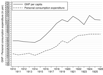
Figure 1: Gross National Product per Capita and Personal Consumption Expenditure (in yen)

Note: This figure shows the gross national product per capita (solid line) and personal consumption expenditure (dashed line) between 1910 and 1926. The prices are deflated using the CPI in 1934-1935 price.

Sources: Created by the author using Ohkawa et. al. (1974, p. 237).

As described, there were short-term business cycles, such as the boom caused by WWI and the subsequent recession. However, taken as a whole, Japan achieved a high economic growth rate relative to other countries in the early 20th century and before WWII (Nakamura 1971, pp. 2–5). As shown in Figure 1, the growth rates of personal consumption expenditure were particularly high during and immediately after WWI, with average growth rates reaching 112% in 1915-19 and 118% in 1920-24. This was a high level even by international standards (Nakamura 1971, p. 27). Given the rapid urbanization, it is therefore necessary to focus on the consumption behavior of urban households when considering the Japanese economy at that time. However, progress has yet to be made in analyzing the consumption behavior (Nakamura 1971, pp. 30–31).

2.2 Tsukishima: A Representative Manufacturing Area

The population in Tokyo City has been growing since the end of the 19th century, and industrialization due to WWI spurred its growth. Tokyo City’s population share increased from 2.5% in 1889 to approximately 4% by 1920. Throughout the 1910s, the percentage of industrial and commercial workers increased in Tokyo City, building the city as a gigantic commercial and industrial place (Tanimoto 2002, p. 8). In fact, Column 1 of Panel A in Table 1 shows that nearly half of the male workers worked in the industrial sector as of 1920 in Tokyo.

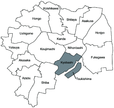
Figure 2: Administrative Wards in Tokyo City

Notes: The name in each lattice indicates the administrative ward in Tokyo. The gray ward indicates the Kyobashi Ward and an island in the Kyobashi Ward indicates Tsukishima. The border surrounded by Asakusa, Honjyo, Nihonbashi, and Fukagawa wards includes the Sumida River. The borders of each ward are based on the administrative district in 1920. Geographical coordinate system is based on JGD2000/(B, L).

Source: Created by the author using the official shapefile (Ministry of Land, Infrastructure, Transport and Tourism, database).

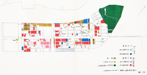
Figure 3: Factories in Tsukishima

Notes: Blocks in green and light green indicate the shipyards. Blocks in red and pink indicate the factories in the machinery sector. Blocks in blue and light blue indicate the factories in the other manufacturing sectors. Blocks in brown are the warehouses. Small circles colored in black and white show the workplaces in the machinery sector and the other manufacturing sectors, respectively.

Source: Department of Health, Ministry of the Interior 1923c, second map. The tone was adjusted by the author using Adobe Photoshop 24.7.0.

The subject of this paper is Tsukishima, an industrial area located southeast of Kyobashi Ward in Tokyo (Figure 2). Column (2) of Panel A in Table 1 shows that Kyobashi had an industrial composition similar to that of Tokyo City in 1920. Column (3) confirms that Tsukishima is a representative industrial area in the city; approximately 68% of male workers were employed in the manufacturing sector. In the same year, there were 214 factories on this island, and approximately 80% of them belonged to the machinery and related sectors. (Department of Health, Ministry of the Interior 1923a, pp 385–389). Figure 3 shows the spatial distribution of factories in Tsukishima as of June 30, 1918. Tsukishima had many machine factories and shipyards, and the workers’ residences were clustered there. The focus of this study is the consumption behavior of these worker households in the industrial sector.

Table 1: Industrial and Family Structures in Tsukishima

Panel A: Industrial structure
Name of survey	(1) 1920 Population census	(2) 1920 Population census	(3) 1920 Population census
Survey area	Tokyo City	Kyobashi Ward	Tsukishima
Survey subject	Complete survey	Complete survey	Complete survey
Survey month and year	October 1920	October 1920	October 1920
Agriculture	1.0	0.6	0.4
Fisheries	0.1	0.3	0.8
Mining	0.4	0.4	0.8
Manufacturing	44.5	45.2	67.7
Commerce	32.4	34.0	16.9
Transport	7.6	10.2	6.1
Public service and professions	11.3	10.2	4.6
Housework	0.3	0.1	0.2
Other industry	2.4	2.0	2.5
Panel B: Demographic structure
Name of survey	(1) 1920 Population census	(2) 1920 Population census	(3) 1920 Population census
Survey area	Tokyo City	Kyobashi Ward	Tsukishima
Survey subject	Complete survey	Complete survey	Complete survey
Survey month and year	October 1920	October 1920	October 1920
Average household size (in person)	4.6	4.7	4.3
Share of married males (%)	38	36	40
Sex ratio (males/females)	1.2	1.2	1.3
0–13 years	1.1	1.1	1.1
14–19 years	1.5	1.7	2.2
20–29 years	1.3	1.4	1.6
30–39 years	1.2	1.2	1.3
40–49 years	1.2	1.2	1.3
50–59 years	1.1	1.1	1.2
60+	0.8	0.8	0.9
Average age of males	25.3	25.3	25.1

Notes:

Panel A: This panel summarizes the industrial structures based on the occupations of male workers measured in the 1920 population census. Each share is calculated as the number of males worked as regular workers in each sector divided by the total number of male workers (in percentage). All the figures do not include the number of unemployed (mugyō sha) males.

Panel B: The average household size is the number of people divided by the number of households. The share of married males is the number of married males living with/without spouses divided by the total number of males (in percentage). The average age of males is calculated using the tables for population by age group reported in the census. Since the tables are open-ended, the class for over 60 years old is rounded as $64.5$ following the range of the former category (i.e., 50–59). All the figures in this panel do not include a small number of quasi-households (jyun setai), which include the person, such as the students in dormitories and the patients in hospitals.

The figures for Tsukishima listed in column 3 of both panels are based on the total sum of statistics of all the blocks (chōme) in Tsukishima (i.e., from Tsukudajima to Tsukishima dōri jyūni chōme).

Sources: Columns 1 and 2 of Panel A use the Statistics Bureau of the Cabinet (1929c, pp. 18–19). Columns 1 and 2 of Panel B use the Statistics Bureau of the Cabinet (1929c, pp. 38–43); Tokyo City Office (1922b, pp. 2–3; 42–46). Column 3 of Panel A uses the Tokyo City Office (1922c, pp. 42–47). Column 3 of Panel B uses the Tokyo City Office (1922a, pp. 26–31); Tokyo City Office (1922b, pp. 2–3; 42–46).

To look more closely at the characteristics of working-class households in Tsukishima, Panel B in Table 1 summarizes the population and occupational statistics from the census. First, the average household size in Tsukishima is $4.3$, similar but slightly smaller than the values of $4.6$ and $4.7$ in Tokyo City and Kyobashi Ward, respectively. The percentage of the married male population is $40$%, which is in the similar range of the figures of Tokyo City ($38$%) and Kyobashi Ward ($36$%). The average age of men in Tsukishima is $25.1$, slightly lower than the figures for Tokyo and Kyobashi. While the sex ratio by age group in Tsukishima shows a similar trend to that of Tokyo and Kyobashi, the ratios for the $14$–$19$ and $20$–$29$ age bins are higher than those. Overall, these statistics reflect the fact that Tsukishima is a typical industrial area and many young male workers were employed there. The slightly smaller household size in Tsukishima can be attributed to the relatively large number of young factory worker households compared to other areas. Given that the percentage of married men is slightly higher in Tsukishima, some of these worker households in their early 20s might had been couples before they started raising children.

Finally, I briefly overview the lives of the factory workers’ households in Tsukishima. Factories and workers’ residences were scattered throughout the island. The factory workers had lived in similar tenements and used the commercial stores and restaurants in the central lot. There were two postal offices, 13 pawnshops, and five moneylenders, and those were scattered throughout the island (Online Appendix Figure A.2). As for medical personnel, there were eight doctors, four dentists, eight obstetricians, and 14 drug stores. The main routes to the mainland were the wooden Aioi Bridge (Aioi bashi) and three ferries (watashi bune). The average daily total number of people using the ferries in 1918 was reported to be $53,318$, accounting for more than twice as many people as the Tsukishima population. These descriptions illustrate Tsukishima as a busy machine industry area during the industrialization.

2.3 Risk-Coping Institutions

Working-class households had been exposed to several risks that led to losses of income at that time. Generally, social insurance, such as health, accident, and unemployment insurance, can help mitigate the idiosyncratic income shocks on the workers. However, comprehensive social insurance systems did not exist in the early 1920s in Japan. The former health insurance was enacted in 1927 and unemployment insurance had not been established throughout the prewar period. Therefore, the workers had basically no public support for their illness, injuries, and joblessness. Instead, they might have used private financial institutions to deal with the idiosyncratic risks.

Several financial institutions were indeed available for working-class households. A representative savings institution for households was the postal savings (yūbin chokin). In Tokyo City, roughly $1.4$ million people had postal savings accounts, covering approximately $67$% of the entire citizens in 1920 (Online Appendix Table A.2). The average savings amount per capita in Kyobashi Ward was $44.5$ yen (Tokyo City Office 1921, pp. 892–893), which is less than one month’s earnings of the skilled-factory workers (Section 3.2). Savings bank (chochiku ginkō) is another famous savings institution among the working class in the 1910s (Ito and Saito 2019, pp. 79–81). The number of people with savings accounts was roughly $1.4$ million, accounting for approximately $58$% of total people in Tokyo (Online Appendix Table A.2). However, $84.8$% of all the depositors were the commerce and miscellaneous workers, and the manufacturing sector shared only $11.5$% in Kyobashi Ward (Online Appendix Table A.3). As described by the Tokyo Institute for Municipal Research, savings bank was a savings institution designed for lower-income workers than factory workers (Tokyo Institute for Municipal Research 1925b, p. 81). This is consistent with the fact that Tsukishima did not have any savings bank branches, while there were two postal offices (Section 2.2). Although another savings institution was the mutual loan association (mujin), it had been used among small business owners and merchants for running their businesses (see Online Appendix A.2 for details).

There also be a few lending institutions. Credit purchases (kakegai) in retail shops were the most popular institution. Although the systematic statistics on credit purchases are unavailable, the THBS households often used credit purchases in various retail shops for rice, fish, vegetables, firewood, and charcoal. I will describe this institution in detail in Section 5. Pawnshop was the popular lending institution among low-income households who might face certain credit constraints. The accessibilities were higher than the other lending institutions: as described, there were $13$ pawnshops in Tsukishima, more than twice the large number of moneylenders. However, the core users of the pawnshops were the low-income working-class households rather than the factory workers (Tokyo City Social Affairs Bureau 1921, p. 9). According to the statistics on the pawnshop users in Tokyo prefecture in 1923, the most representative users were the day laborers and workers classified as “miscellaneous”, accounting for $63.4$% of all users. In contrast, those for agriculture, commerce, and manufacturing sectors were only $1.7$, $19.5$, and $15.6$%, respectively (Tokyo Institute for Municipal Research 1926, p. 25). The inexpensive article means that pawnshops were used to deal with very short-run necessities only. Among the pawnshops of Kyobashi, for example, the average amount per case was $7.8$ yen which accounts for $14$% of the monthly earnings of the THBS households. This means that the average redemption rate was substantially high: among $88$ pawnshops in Kyobashi, it was approximately $94$% in 1920 ($401,222$ cases/$427,265$ cases) (Tokyo City Office 1922b, pp. 888–889). While the pawnshops were the famous lending institutions, they might not offer a sufficient amount of temporary income.

Other lending institutions are money lenders (kinsen kashitsuke gyō) and credit unions (shinyō kumiai). Generally, moneylenders were used by business owners with very high-interest rates (Shibuya 2000, pp. 184; 248). Similarly, the coverage of the credit unions was substantially low, say a few percentage points of the male workers in the manufacturing sector (Online Appendix A.2). Informal gifts may be another type of risk-coping institution, although systematic statistics are not available. A household survey on the 185 factory-worker households in Tokyo suggests that the share of average monthly gifts in total income was approximately $3$% in November 1922 (Social Affairs Division 1925, pp. 58-59). Although this means that the gifts comprised a few percentage points of the monthly income, whether these informal income transfers had functioned as mutual aid is unclear.

To summarize, while there were several institutions, the available institutions for the factory-workers were few in the practical sense. For savings institutions, the postal savings might have been the best available devices for Tsukishima workers. Regarding lending institutions, credit purchase is the plausible device among factory workers. Although pawnshops were the most accessible financial institutions, they might not provide sufficient money as the articles were usually inexpensive. The factory workers in Tsukishima might have combined these risk-coping devices to deal with the idiosyncratic income shocks.

3 Data

This section offers a set of descriptive analyses to understand the characteristics of the data used in the study. I give an overview of the Tsukishima Survey in Section 3.1. I then utilize the statistics from the complete surveys in Section 3.2 to assess the representativeness of the sample households. In Section 3.3, I explain my data aggregation method to overcome the potential measurement error issue. The variables used, the trend in income and expenditure, and variations in idiosyncratic shocks are introduced in Section 3.4.

3.1 Tsukishima Household Budget Survey

The Tsukishima Survey was the first urban social survey conducted in Japan by the Ministry of Home Affairs around 1919. The purpose was to investigate the status of the lives of urban worker households amid the rapid progression of industrialization throughout WWI. It was designed as a field survey consisting of multiple survey items on the worker households, and the household budget survey (hereafter THBS) included in. The Ministry of Interior published a report on the Tsukishima Survey in 1921, which contains some aggregated information on the target households. However, the main interest of this current study is the variations in the consumption and income in each household, meaning that household-level budget information is required.

Fortunately, the household budget book (kinsendeiri hikaechō) gathered in the THBS is preserved in the archives of the Ohara Institute of Social Research (hereafter, OISR). These budget books were transferred to the OISR by Iwasaburo Takano, who was responsible for the Tsukishima Survey as a member of the 7th Section of the Health and Hygiene Research Committee of the Ministry of Home Affairs and became the first director of the OISR.

I corrected and digitized all the 40 THBS budget books for the factory worker households that were included in the official report of the Tsukishima Survey. During the study period, each household recorded their income and expenses daily in a budget book. Notably, a survey office was set up in Tsukishima, where a few surveyors lived and were closely connected with the survey households. Furthermore, weekly administrative meetings were held to discuss the progress of the survey (Miyoshi 1980, p. 38). This confirms that the information in these budget books is reliable and that the THBS budget dataset ensures a quality that allows quantitative analysis.

3.2 Sample Characteristics

Analytical Sample

I use the semi-monthly and monthly panel datasets for my baseline analyses. Among the 40 THBS households, there are five cross-sectional units in the semi-monthly and monthly data. The estimation strategy used for testing consumption smoothing and risk-coping behaviors requires the panel structures (Section 4). Thus, I excluded these five cross-sectional units, leaving 35 THBS households. Next, a household with incomplete income information, which is necessary data for my analysis, is removed. I also exclude a household for which no information on payments to the credit purchases was recorded. Finally, I excluded the small number of budget books created at both edges of the survey periods to aggregate the daily to semi-monthly dataset that I will explain in detail in the next section (Section 3.3). Consequently, my THBS sample includes 33 households with panel structures from 12th January to 11th November 1919. Online Appendix B.3 presents the finer details of the original data structure and trimming.

Before analyzing the representatives of the THBS sample, I assess the potential selection bias due to attrition of the units. The panel units with shorter (longer) time-series observations might have different preferences on the consumption than those with longer (shorter) time-series observations. In other words, the households with shorter panels should have similar family size characteristics to those with more extended panels. To test this potential issue, I regressed an indicator variable for the shorter panel units on the family size variables using the THBS sample. Online Appendix Table B.2 summarizes the results. All the estimated coefficients on the covariates are close to zero and statistically insignificant, and this result is robust to changing the thresholds. The Wald statistics support the null results, which are robust to using different thresholds such as first quantile, median, and third quantile. This result supports the evidence that the family structure, representing the household’s preference, is independent of the unbalancedness in my analytical sample.

Representativeness

Table 2: Assessing Representativeness: Tsukishima Household Budget Survey

Panel A: Manufacturing sector
Name of survey	(1) 1919 Statistics of	(2) 1920 Tsukishima Factory		(3) The THBS
	National Police Agency	Survey
Survey area	Tsukishima	Tsukishima		Tsukishima
Survey month and year	December 1919	November 1920		1919
Survey subject	All factories with	All factories with # of		33 households
	# of workers $\geq 15$	workers $\geq 15$	workers $<15$
Textile	0.2	2.9	0.0	0
Machinery	87.4	85.3	91.8	93.9
Chemical	1.1	5.9	5.5	0
Food	1.2	1.5	0.0	3.0
Miscellaneous	10.2	4.4	2.7	3.0
Observations	$7,647$ workers	68 factories	146 factories	33 heads
Panel B: Family structure
Name of survey	(1) 1920 Population	(2) 1919 Statistics of	(3) The THBS
	Census	National Police Agency
Survey area	Tsukishima	Tsukishima	Tsukishima
Survey month and year	October 1920	December 1919	1919
Survey subject	Complete survey	Complete survey	33 households
Average household size	4.3	4.3	4.3
Sex ratio	1.3	1.2	1.2
Household size (% share)
1	6.0	–	0
2	16.7 (18.7)	–	15.2
3–5	50.8 (57.1)	–	57.6
6–8	21.5 (24.2)	–	27.3
9+	4.9	–	0
Pearson $\chi^{2}$ statistic $p$-value	–	–	0.948
Panel C: Monthly earnings
Name of survey	(1) The THBS		(2) Manufacturing Census
Survey area	Tsukishima		Tokyo City
Survey/equivalent year	1919		1919
Survey subject	THBS heads		Male factory workers
	(Ave. age: 33.2)		in machinery factories
			(Age range: 30-40)
Average monthly earnings	52.7		55.0
	95%CI [48.0, 57.4]

Notes: Panel A: Column 1 shows the share of factory workers to the total factory workers in each sector (in percentage). The number of factory workers includes female and male factory workers in the 68 factories, with 15 workers and more. Column 2 indicates the share of factories to the total number of factories in each sector by factory size (in percentage). Column 3 summarizes the manufacturing sectors for the heads of the THBS. The definition of classification in the Statistics of the National Police Agency (column 1) is used in columns 2 and 3. Following this definition, several “woodworking” factories measured in the Tsukishima Factory Survey are included in the machinery sector in column 2, as it consists of shipbuilding and wooden pattern factories. The report also supports that the wooden patterns are used in the casting process and shall be regarded as one of the machinery sector (Department of Health, Ministry of the Interior 1923a, pp. 388–389).

Panel B: The first and second rows in columns 1 and 2 show the average household size and sex ratio measured in the 1920 Population Census and Statistics of the National Police Agency of 1919, respectively. The third to eighth rows in columns 1 and 3 show household size distributions in the census and the THBS sample, respectively. The figures in parentheses in Column (1) are the percentage share for family size bins between 2 and 8 people. The ninth row in column 3 shows the $p$-value from the Pearson $\chi^{2}$ test for the equality of the household size distributions between 2 and 8 people. The share in each household size bin measured in the census is used as the theoretical probability in calculating the test statistic (Online Appendix B.5).

Panel C: Column 1 lists the average monthly earnings of the THBS heads calculated using the adjusted monthly panel dataset. Gaussian-based 95% confidence interval (CI) using bootstrap standard error is reported in the brackets. Column 2 shows the average monthly wage of the male factory workers in the skilled age range (30-40 years old) in machinery factories in Tokyo City. This figure is calculated using the average monthly wage and average monthly ancillary wage measured in the manufacturing censuses. All the wage statistics are deflated using the CPI for cities provided by Ohkawa et al. (1967, p. 255). Online Appendix B.6 summarizes the finer details of the process of this wage estimation.

Sources: Panel A: Column 1 uses the National Police Agency (1920b, p. 236). Column 2 uses the Department of Health, Ministry of the Interior (1923a, p. 385–386). Column 3 uses the Department of Health, Ministry of the Interior (1923a, p. 154). Panel B: Column 1 uses the Tokyo City Office (1922a, pp. 26–31; 262–283); Tokyo City Office (1922b, pp. 2–3; 42–46). Column 2 uses the National Police Agency (1920b, p. 53). The figures in column 3 are calculated by the author using the THBS dataset. Panel C: Column 1 uses the THBS dataset. Column 2 uses the Tokyo City Statistics Division (1926a, pp. 16; 244–245); Tokyo City Office (1921, pp. 726–757).

By using the manufacturing and population censuses, I first assess the representativeness of the THBS sample in Tsukishima.

Panel A of Table 2 summarizes the share of male workers in the manufacturing industry by sector. Statistics of the National Police Agency (hereafter SNPA) focusing on factories with more than or equal to 15 workers show that roughly 90% of male workers had been engaged in the machinery sector in 1919 (column 1). Column 2 summarizes the statistics in the manufacturing census conducted in the Tsukishima Factory Survey. The proportion of machine factories is $85$% in larger factories and $92$% in smaller factories. Thus, both columns indicate that most of the male workers in Tsukishima worked in the machinery sector. In column 3, I confirm that the THBS heads’ occupations show a similar proportion: $94$% worked in the machinery sector. In fact, the report states that “It is not too much to say that most of the industry in Tsukishima is machinery. Therefore, to describe the labor situation in Tsukishima, it is sufficient to describe its machinery industry” (Department of Health, Ministry of the Interior 1923a, p. 389). Figure 3 illustrating many machinery factories supports this statement for Tsukishima. For the other sectors, the THBS includes a few heads who worked in food and miscellaneous sectors, and the proportions are similar to those listed in column 2.

Panel B of Table 2 summarizes the family structure. The average household sizes are identical in the Population Census ($4.3$ in column 1), SNPA ($4.3$ in column 2), and THBS ($4.3$ in column 3). In addition, the sex ratio is similar across the surveys ($1.2$–$1.3$). The number of people in the THBS households ranges from 2 to 8, meaning the THBS sample does not include single or very large households. In other words, the THBS mainly focuses on the consumption behavior in couples and households with a few children. For this household size range, the Pearson $\chi^{2}$ test does not reject the null of equality in the household size distributions with $p$-value = $0.948$. This means that the THBS sample reasonably approximates the distribution of family households in Tsukishima. This confirms the validity of the statement in the report that the THBS households can be “regarded as representative of the family form in Tsukishima” (Department of Health, Ministry of the Interior 1923a, p. 145). Online Appendix B.5 illustrates the household size distributions in finer detail.

The official report of the Tsukishima Survey suggests that roughly nine out of ten factory workers in the skilled-age range were classified as skilled workers. Roughly six of those skilled workers were employed in the middle- to large-scale factories, and three worked in small-scale factories. Given this fact in Tsukishima, the THBS was designed to investigate the budgets in skilled workers’ households. The average THBS head’s age is 33, which is indeed in the skilled workers’ representative age range of the 30s in the machinery factories (Kitazawa 1924). Column 1 of Panel C in Table 2 indicates that the average monthly earning of the THBS heads is $53$ yen. In Column 2, I calculated the average monthly earning of male machinery factory workers in the skilled-age range using the manufacturing censuses for the entire city, which shows only $2$ yen higher earnings (i.e., $55$) than the THBS heads’ earnings. This provides evidence that the monthly earnings of the THBS heads and skilled workers’ households in Tsukishima are materially similar. Therefore, the THBS households can be useful in inferring the mean tendency of those households.

3.3 Aggregation

Measurement Error

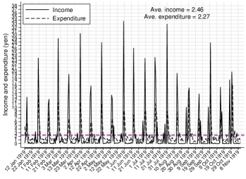
(a) Daily panel dataset:
income and expenditure

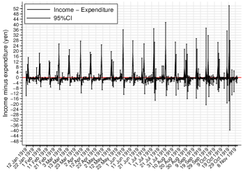
(b) Daily panel dataset:
net income

(c) Semi-monthly panel dataset:
income and expenditure

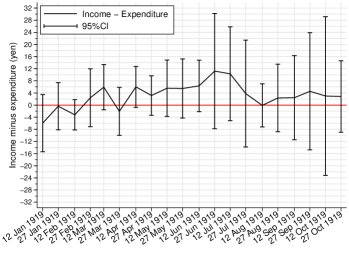
(d) Semi-monthly panel dataset:
net income

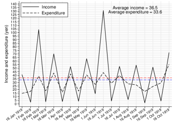
(e) Unadj. semi-monthly panel dataset: income and expenditure

(f) Unadj. semi-monthly panel dataset: net income

Figure 4: Relationships between Average Income and Expenditure
by Different Time-series Frequencies

Note: Figure 4a, 4c, and 4e illustrate the time-series plots of the average daily, semi-monthly, and unadjusted semi-monthly income and expenditure, respectively. Figure 4b, 4d, and 4f illustrate the time-series plots of the average daily, semi-monthly, and unadjusted semi-monthly income minus expenditure. Figures 4a and 4b shows the daily data between 12th January and 11th November 1919. The (adjusted) semi-monthly series defines the 12-26th for the first and 27-11th for the second half. Thus, Figures 4c and 4d show the semi-monthly series calculated using the daily data between 12th January and 11th Novemeber 1919. The unadjusted semi-monthly series uses the 15th of each month as a threshold. Figures 4e and 4f show the unadjusted semi-monthly series calculated using the daily data between 15th January and 31st October 1919.

Source: Created by the author using the THBS sample.

It is necessary to summarize the daily budget information into a more extended time range because household needs a set of time to smooth their consumption given a realiszed amount of income. To explore the reasonable way to aggregate the THBS dataset, I first overview the daily time series on the total income and expenditure. Figure 4a shows that the head’s income had been paid twice monthly: the semi-monthly wages were paid on the middle (14–16th) and last day (30th or 31st). Importantly, Figure 4a indicates that the households expensed much of their income just on the payday and spent the rest of the payment little by little until the next payday. In other words, the expenditures had never clearly increased just before the paydays. This means that the households had made their consumption decisions (schedules until the next payday) based on the income they obtained. Notice that the calendar (semi-)monthly aggregation can not reflect this household behavior because the calendar (semi-)month does not place the payday at the beginning of its cell. Another source of measurement error is the shift of the payday: the payday for the latter half of a month was sometimes set on the first date of the following month. Although this shift did not occur frequently, the calendar month cell shall contain a substantial noise from the shift as it leads to the cells including more (three paydays) and fewer (one payday) payments than normal. Nelson (1994) suggests that this sort of mismatching in the timing of income and expenditure tends to induce the type II error in the test of consumption smoothing.

Adjustment

To match income and expenditure data precisely, I first consider aggregating the daily data into semi-monthly series. Specifically, I aggregate the daily observations between the 12th and 26th for the first half and those between the 27th and 11th of the next month for the second half. This range is based on the fact that almost all of the paydays in the second half of a month measured in the THBS dataset, are 27th–31st.

Figure 4c shows the time-series plots of the income and expenditure from this adjusted semi-monthly panel dataset, whereas Figure 4e illustrates the unadjusted (calender) semi-monthly series using the 15th of each month as the threshold of the semi-month. Clearly, Figure 4e provides very rough measures of both income and expenditure due to the measurement errors from the misadjustment of paydays. The most significant improvement in Figure 4c is that the expenditure can chase the income in each month, reflecting the households’ consumption behaviors based on their income measured in the exact timing. Given the improvements in both income and expenditure measures, the net income series shows a much smoother trend in Figure 4d, which are not available under the unadjusted definition (Figure 4f). In Section 4.1, I will demonstrate how these measurement errors in the unadjusted dataset attenuate the estimates.

3.4 Data Description

Variables

The THBS budget book has two primary sections: expenditure and income. I digitized records in each category following the categorization used in the official report of the Tsukishima Survey. Panel A of Table 3 lists the $11$ subcategories for expenditures: food, housing, utilities, furniture, clothes, education, medical, entertainment, transportation, gifts, and miscellaneous. These variables are used to test the smoothness of these consumptions. I consider five net income categories: net savings, net insurance, net borrowing, net credit purchase, and net gifts to investigate the risk-coping strategies. Net variables are defined as the income minus expenditure in each category; for example, net savings refers to the difference between the withdrawal amount and deposits to savings. I also consider the sales of miscellaneous goods and labor earnings from the family members except for the head to test the contribution of the asset sales and intrahousehold labor-supply adjustments. Panel B of Table 3 summarizes these variables.

It is important to take into account the possibility of changes in preferences that may occur as a result of alterations in family size (Jappelli and Pistaferri 2017). Fortunately, the archives of the Tsukishima Survey include the sheets documenting the changes in household composition (Kazoku idō hyō). I found that the size of households had been stable over time: one household experienced changes in the number of family members due to the birth of a son during the sample periods. This supports the evidence that the preference shifts had rarely occurred among the THBS households. Although family size is included in all regressions to be conservative, it has little effect on the results. Panel C of Table 3 shows the summary statistics on the family size variable.

Table 3: Summary Statistics

Panel A: Variables for testing consumption smoothing (in yen)
	Semi-monthly Panel Dataset				Adj. Monthly Panel Dataset
	Level		Log		Level		Log
	Mean	Obs.	Mean	Obs.	Mean	Obs.	Mean	Obs.
Total expenditure	34.5	289	3.4	289	61.1	162	4.0	162
Food	10.9	289	2.3	270	19.5	162	2.8	152
Housing	2.7	289	1.6	134	4.9	162	1.8	118
Utilities	1.2	289	-0.1	232	2.2	162	0.5	147
Furniture	0.4	289	-1.6	177	0.7	162	-1.2	126
Clothes	2.8	289	0.3	248	5.0	162	1.0	148
Education	0.7	289	-0.6	201	1.3	162	-0.2	135
Medical	1.7	289	0.2	269	3.0	162	0.7	152
Entertainment	1.4	289	-0.1	255	2.5	162	0.5	150
Transportation	0.4	289	-1.3	195	0.8	162	-0.9	125
Gift	3.1	289	0.5	243	5.6	162	1.2	148
Miscellaneous	0.5	289	-1.3	222	0.9	162	-0.9	140
Disposable income	37.6	289	3.5	278	67.3	162	4.1	159
Panel B: Variables for testing risk-coping mechanisms (in yen)
	Semi-monthly Panel Dataset			Adj. Monthly Panel Dataset
	Mean	Std. Dev.	Obs.	Mean	Std. Dev.	Obs.
Panel B-1: Savings, insurance, borrowing, and gifts
Net savings	-0.01	3.97	289	-0.02	5.52	162
Net insurance	-0.03	6.67	289	-0.05	8.97	162
Net borrowing	0.31	5.03	289	0.61	7.32	162
Net credit purchase	-2.47	11.33	289	-4.67	19.38	162
Net gifts	-2.04	6.11	289	-3.56	9.20	162
Panel B-2: Labor supply adjustments & sales of miscellaneous assets
Other family member’s earning	3.74	6.11	289	6.72	14.79	162
Sales of assets	0.02	0.12	289	0.04	0.15	162
Panel B-3: Income variable
Head’s earning	29.43	18.11	289	52.70	30.30	162
Panel C: Family size (people)
	Semi-monthly panel dataset
	Mean	Std. dev.	Min	Max	Obs.
Number of family members	4.3	1.6	2.0	8.0	289
Panel D: Health shocks
	Semi-monthly panel dataset
	Mean	Std. dev.	Min	Max	Obs.
Number of days with illness (head)	0.1	0.8	0	11	254
Number of days with illness	0.2	1.7	0	16	254
(the other family members)

Notes:

Panel A: The summary statistics of the variables used to test the consumption smoothing for the 33-panel units in the semi-monthly and adjusted monthly panel datasets are shown in this panel. Disposable income is the total income minus tax payments.

Panel B: This panel shows the summary statistics of the variables used to test the risk-coping strategies for the 33-panel units in the semi-monthly and adjusted monthly panel datasets. Each net income variable is defined as the difference between income and expenses. “Net savings” refers to the difference between the amount withdrawn and the total deposits. “Net insurance” refers to the amount received from insurance minus the expenses paid for insurance. “Net borrowing” refers to the amount of borrowing minus the debt payments. “Net credit purchase” refers to the amount of credit purchases minus credit redeemed. “Net gifts” refer to the total received amounts, including both pecuniary and non-pecuniary gifts, minus the payments for gifts. “Other family member’s earnings” refers to the total income earned by all family members except for the head of the household. “Sales of assets” includes the sale of daily miscellaneous goods such as newspapers and empty bottles.

Panel C: The summary statistics of the family size variable for the 33-panel units in the semi-monthly panel dataset are listed. The statistics for the adjusted monthly panel dataset are not reported because they are materially similar to those for the semi-monthly panels.

Panel D: The summary statistics of the number of days with illness for family members are listed. Since both are lagged variables, the initial time period in all the units is omitted. Similarly, a household with two semi-month observations is excluded. Similarly, .

Sources: Created by the author from the THBS sample.

Trend

Next, I overview the time-series figures to evaluate the representativeness of my THBS dataset. Figure 4c shows a weak increasing trend in the average income. This is consistent with the macroeconomic trend in the nominal income during this period. This trend in earnings was, however, offset by the steep inflation under the expansions after the war (Section 2.1). In Figure 4d, the deviation of expenditure from income in January must capture the expenses on the goods for the New Year events. The gaps in June to the first half of July may reflect the payments of bonuses. The humps in March may reflect the preparation for the new fiscal and academic year from April, meaning that the increased income in this month may suggest a higher proportion of temporary income from withdrawals and loans. These support the evidence that the budget data from the THBS households can capture the macroeconomic trends.

Idiosyncratic Shocks

Online Appendix Figure B.11 illustrates the residuals from the regression in the first difference in semi-monthly income on the first difference in aggregate semi-monthly income. While the residuals satisfy the zero-average property, they occasionally take large negative and positive values, suggesting that the workers had experienced idiosyncratic income shocks in some cells. Regardless of favorable or adverse shocks, these cells that deviated from mean tendency are helpful in investigating how those households coped with the idiosyncratic shocks. Despite this, it is helpful to focus on the illness as it is the least predictable shock (Gertler and Gruber 2002). Although joblessness is another shock, the THBS heads rarely changed their occupation during the survey period as they are the skilled workers who were less likely to move to other jobs. In contrast, fortunately, the illness among the THBS family is documented systematically. As explained in Section 2.3, the comprehensive health insurance system was unavailable then. Moreover, the sanitary conditions in the cities were low, leading to higher mortality rates. The official report indeed mentioned the fact that the workers in the machinery factories in Tsukishima had faced the risk of diseases (Department of Health, Ministry of the Interior 1923a, p. 14).

Considering this, I first provide the overall results from the specification using the changes in earnings as the idiosyncratic income shock in Sections 4.1 and 4.2. I then consider the structure behind the adverse income shocks using the heads’ temporary illness to investigate the households’ consumption and risk-coping behaviors in Section 4.3. Panel D of Table 3 shows the summary statistics on the health shock variables used.

Risk Preferences

This study investigates consumption smoothing behaviors among homogeneous households, say the skilled factory workers’ households in the machinery sector in Tsukishima. This empirical setting is useful because the different attitudes toward risks among households may lead to bias in the standard risk-sharing regressions. Following Schulhofer-Wohl (2011), I tested whether the earnings of the heads who worked in a few specific factories or sectors showed different responses to the aggregate shocks. Specifically, I consider the heads who worked in large-scale or governmental factories to have potentially different risk preferences because those workers might have lower risk tolerance than those who worked in smaller enterprises. I confirmed that the sensitivities to the aggregate shocks are materially similar in both groups in the statistical sense. This result is unchanged if I assume that a few heads who worked in the smithing factory or in the non-machinery sectors had different risk preferences. This supports the evidence that conditional on the household fixed effects, it is plausible to assume that the THBS households shared similar risk preferences. Online Appendix B.10 summarizes the finer details of this analysis.

4 Empirical Analysis

4.1 Consumption Smoothing

Estimation Strategy

I consider a linear fixed-effects model designed to test the consumption smoothing. Online Appendix C.1 provides the conceptual framework and the derivation of my empirical specification. For household $i$ in time $t$, the reduced form equation is characterized as follows:

$$\log c_{i,t}=\gamma\log y_{i,t}+\delta x_{i,t}+\mu_{i}+\phi_{t}+u_{i,t},$$ (1)

where $c_{i,t}$ is consumption, $y_{i,t}$ is disposable income, $x_{i,t}$ is the family size control, $\mu_{i}$ is the household fixed effect, $\phi_{t}$ is the semi-month fixed effect, and $u_{i,t}$ is a random error term. The household fixed effect captures the time-constant unobservable factors such as permanent income and consumption preference. The time-fixed effect effectively removes the unobservable macroeconomic shocks and trends described in Section 3.4. The estimate of $\gamma$ suggests income elasticity, which can range from zero for perfect insurance to one for the absence of insurance. The cluster-robust variance-covariance matrix estimator is used to deal with heteroskedasticity and serial dependency (Arellano 1987).

Results

Table 4: Results of Estimating Income Elasticities

	(1) Semi-monthly Panels			(2) Adj. Monthly Panels			(3) Unadj. Monthly Panels
	Disposable income		Obs.	Disposable income		Obs.	Disposable income		Obs.
	Coef.	Std. error		Coef.	Std. error		Coef.	Std. error
Total consumption	0.358	[0.033]***	278	0.548	[0.065]***	159	0.261	[0.054]***	144
Food	0.136	[0.030]***	259	0.436	[0.088]***	149	0.100	[0.072]	135
Housing	0.099	[0.415]	134	0.291	[0.243]	118	-0.263	[0.167]	126
Utilities	-0.003	[0.138]	223	0.431	[0.149]***	144	0.197	[0.333]	133
Furniture	0.426	[0.223]*	169	0.943	[0.335]***	123	0.250	[0.339]	114
Clothes	0.378	[0.190]*	238	0.374	[0.324]	145	0.806	[0.262]***	135
Education	0.070	[0.092]	194	0.337	[0.212]	133	0.093	[0.213]	125
Medical expenses	0.039	[0.066]	258	0.498	[0.196]**	149	-0.128	[0.094]	135
Entertainment expenses	0.355	[0.109]***	244	0.484	[0.148]***	147	-0.049	[0.199]	134
Transportation	0.278	[0.110]**	187	0.635	[0.190]***	124	0.362	[0.290]	117
Gift	0.523	[0.106]***	234	0.599	[0.115]***	146	0.622	[0.305]*	133
Miscellaneous	-0.076	[0.147]	214	0.549	[0.184]***	137	0.246	[0.267]	129

***, **, and * denote statistical significance at the 1%, 5%, and 10% levels, respectively. Standard errors in brackets are clustered at the household level.

Notes: This table shows the results of equation 1: the regressions of the 11 measures of log-transformed consumption on log-transformed disposable income as well as on the family size control, household-fixed effect, and time-fixed effect. Columns 1, 2, and 3 show the results for the semi-monthly, adjusted monthly, and unadjusted monthly panel datasets, respectively. The estimated coefficients on log-transformed disposable income are listed in the column named “Coef.”.

Column (1) of Table 4 presents the results from the semi-monthly panel dataset. In the total consumption, the estimated coefficient is $0.358$. This means that a one percentage point decrease in disposable income decreases the total expenditure by $0.36$ percentage point, suggesting that the factory worker households could not thoroughly smooth their consumptions. Among the subcategories, the food, furniture, clothes, entertainment, transportation, and gifts expenditures are not well-insured. This implies that the households are likely to cut off (increase) their expenses on these categories when they face adverse (favorable) income shocks. The estimates suggest that the expenses on furniture and clothes are relatively sensitive to the shocks ($0.426$ and $0.378$, respectively). This is consistent with the fact that both categories are luxury categories. Similarly, the estimate for gifts shows a large magnitude ($0.523$) because the expenses on the other households are essentially optional. The estimates for the entertainment and transportation expenses are slightly smaller but statistically significant ($0.355$ and $0.278$). This also makes sense, given that these expenses are related to family travel and theatergoing. Importantly, the estimate for food categories is statistically significant but much smaller ($0.136$). This implies that the households might have had some means to deal with idiosyncratic shocks to smooth their expenses on food. I will return to this point later.

Next, I present the results for the adjusted monthly panel dataset in Column (2) to see whether the income elasticities changed in monthly frequency, a longer span than the semi-monthly frequency. Not surprisingly, the adjusted monthly series yields greater estimates than the semi-monthly series. The estimate for total consumption is now $0.548$, which is roughly $1.5$ times greater than that from the semi-monthly panel data. Generally, the panels with short-run time bins are more likely to be influenced by unexpected shocks in consumption, which tends to attenuate the income elasticity (Nelson 1994). In this case, however, the estimates for the adjusted monthly panels are greater than those for the semi-monthly panels across almost all subcategories. The clothes category alone shows a similar but statistically insignificant estimate. This may reflect the cases in which the workers bought their work clothes for the new season. Although such a replacement of work clothes has not occurred frequently (i.e., semi-monthly), this means that the clothes category includes both luxury and necessary items, which may increase the standard error of the estimate.

A few subcategories turn out to be statistically significantly positive: utilities and medical expenses. The estimate for the utility category is relatively large. Given that the sample period includes the winter season, this reflects the households’ behavior of reducing their expenses on firewood and charcoals in economic hardship because those prices were relatively high. The medical categories include the fee for bathing (yuya), typical for working-class people. This indicates that reducing the frequency of taking baths was relatively easy. By contrast, a few subcategories are not sensitive to the idiosyncratic shocks over different time-series frequencies. The estimates for the housing and education categories are not statistically significant in both semi-monthly and adjusted monthly series. This may reflect that the rent payment and school fees were fixed and paid once per month.

Overall, I found that the estimated income elasticity is smaller in the semi-monthly than in the adjusted monthly series. In the total consumption, the estimated coefficient is $0.36$ in the semi-monthly panels, while that is $0.55$ in the adjusted monthly panels. One potential explanation behind this difference is that the available sources of temporary income have been limited, and those sources are not useful for compensating for adverse income shocks lasting for at least one month. In other words, while the household might have been able to compensate for their income losses for a few weeks, they could not do so for several weeks, presumably because of borrowing constraints and/or a limited amount of liquidity assets. The most noticeable example is the food category, which comprises the largest portion of the expenditure (Panel A of Table 3). The estimate for the food category is $0.14$, which is more than three times smaller than the estimate from the adjusted monthly series ($0.44$). This implies that the households’ food consumption is likely to be insured in a few weeks but not over one month. I will delve into the mechanism behind this behavior in the following subsections.

Finally, I assess the validity of the aggregation used in this study. Adjusting the aggregate data to account for the timing of paydays reveals more transparent relationships between income and expenditure than the unadjusted data (Section 3.3). To demonstrate this mechanism, I listed the estimates from the unadjusted monthly panel dataset in Column (3). The estimate for the total consumption is $0.261$, roughly half of the estimate from the adjusted series ($0.548$). In addition, most subcategories show systematically smaller estimates than those from the adjusted data listed in Column (2) and are statistically insignificant. These estimates are clearly odd, with several subcategories taking values close to one or large negative values. Those are no longer economically interpretable. This means that measurement errors in the unadjusted aggregation lead to attenuation bias, which results in false negatives in most of the consumption categories and may cause critical issues in statistical inference for a few subcategories.

4.2 Risk-coping Mechanisms

Preceding results suggest that the skilled workers’ households in Tsukishima were less likely to smooth their consumption. The estimated elasticities, however, become smaller when I focus on the semi-monthly frequency. Specifically, food expenditure is likely to be insured within at least half a month. The workers might have dealt with their shorter-run shocks relatively well but could not cope with the longer-run shocks. In this section, I test the mechanisms behind their smoothing behavior using several variables on the risk-coping devices.

Estimation Strategy

To test the roles of risk-coping strategies, I employ the empirical specification suggested by Fafchamps and Lund (2003). For household $i$ at time $t$, the specification is characterized as follows:

$$r_{i,t}=\kappa\tilde{y}_{i,t}+\eta x_{i,t}+\nu_{i}+\zeta_{t}+\epsilon_{i,t},$$ (2)

where $\tilde{y}_{i,t}$ is head’s earning, $x_{i,t}$ is the family size control, $\nu_{i}$ is the household fixed effect, $\zeta_{t}$ is the time fixed effect, and $\epsilon_{i,t}$ is a random error term. Online Appendix C.1 summarizes the derivation of this specification. I prefer to use the head’s income instead of the disposable income in equation 2 to avoid the potential endogeneity. As for $r_{i,t}$, I consider several variables to overview the wide variety of risk-coping strategies. These include the net income on savings, insurance, borrowing, credit purchases, and gifts. Each net variable is defined as the difference between income and expenses. The estimates of $\kappa$ are expected to be negative since net income becomes negative in good times but positive in unfavorable times. I also consider the sales of miscellaneous goods and the earnings of all the family members except for the head because asset sales and intra-household labor supply adjustments may play a role in mitigating the idiosyncratic shocks as alternative risk-coping strategies (Udry 1995; Blundell et al. 2016). The estimated coefficients for the sales and labor supply adjustment variables are expected to be negative, reflecting additional earnings when the head’s income is reduced.

Results

Table 5: Results of Testing the Risk-Coping Mechanisms

	(1) Semi-monthly Panels			(2) Adj. Monthly Panels
	Head’s earning		Obs.	Head’s earning		Obs.
	Coef.	Std. error		Coef.	Std. error
Panel A: Savings, insurance, borrowing, and gifts (yen)
Net savings	-0.043	[0.018]**	289	-0.042	[0.018]*	162
Net insurance	0.001	[0.013]	289	0.015	[0.024]	162
Net borrowing	-0.021	[0.027]	289	0.036	[0.036]	162
Net credit purchase	-0.128	[0.039]***	289	-0.017	[0.059]	162
Net gifts	-0.052	[0.019]**	289	-0.015	[0.014]	162
Panel B: Labor supply adjustments & sales of miscellaneous assets (yen)
Other member’s earnings	0.001	[0.010]	289	0.038	[0.024]	162
Sales of assets	-0.000	[0.000]	289	0.000	[0.000]	162

***, **, and * denote statistical significance at the 1%, 5%, and 10% levels, respectively. Standard errors in brackets are clustered at the household level.

Notes:

This table shows the results of equation 2: the family size control, household fixed effects, and time-fixed effects are included in all the regressions. Columns 1 and 2 show the estimates for the semi-monthly and adjusted monthly panel datasets, respectively. The estimated coefficients on the head’s earnings are listed in the “Coef.” columns.

Panel A: Each net income variable is defined as the difference between income and expenses. “Net savings” refers to the difference between the amount withdrawn and the total deposits. “Net insurance” refers to the amount received from insurance minus the expenses paid for insurance. “Net borrowing” refers to the amount of borrowing minus the debt payments. “Net credit purchase” refers to the amount of credit purchases minus credit redeemed. “Net gifts” refer to the total received amounts, including both pecuniary and non-pecuniary gifts, minus the payments for gifts.

Panel B: “Other family member’s earnings” refers to the total income earned by all family members except for the head of the household. “Sales of assets” includes the sale of daily miscellaneous goods such as newspapers and empty bottles. All dependent variables are in yen.

Table 5 presents the results. Columns (1) and (2) summarize the results for the semi-monthly and adjusted monthly panel datasets, respectively. Panel A shows the results for the net income variables, whereas Panel B shows those for the labor supply adjustments and sales of assets.

The estimated coefficient for the net savings is negative and statistically significant in Column (1). The estimate suggests that a one yen decrease (increase) in the head’s earnings increases (decreases) the net income from savings by $0.043$ yen. The estimate from the monthly series is similar ($0.042$), albeit weakly statistically significant (Column (2)). This is basically consistent with the historical fact that many workers had savings accounts both in postal savings and savings banks at that time (Section 2.3). However, the estimated magnitude is small, suggesting that the withdrawals from savings did not provide sufficient amounts of temporary income to compensate for the losses of earnings.

The estimates for the insurance category are close to zero and statistically insignificant in both columns. The budget books indicate that the primary source in category is the mutual loan associations (mujin). As explained in Section 2.2, these associations’ rules were unsuitable for compensating the idiosyncratic shocks. A suggestive case is that a THBS household won a lottery and got $100$ yen in a monthly cell, which is clearly independent of the worker’s earnings.

For the net borrowing category, the estimated coefficients are close to zero and statistically insignificant in both columns. Section 2.2 shows that pawnshop was the popular lending institution, especially for the low-income households. Although THBS households occasionally used pawnshops, they never used them frequently. This makes sense because the THBS households can not be categorized as the low-income working class.

The estimated coefficient for the net income from credit purchases is negative and statistically significant in Column (1). The estimate suggests that a one yen decrease (increase) in the head’s earnings increases (decreases) the net income from credit purchases by $0.13$ yen. This magnitude is larger among the other categories. According to the THBS budget books, the credit purchases were mostly used to buy rice, fish, vegetables, and fuels (firewood and charcoal). Since rice, a staple food, is usually an expensive item, credit purchases might have played an important role among these households. While this provides a suggestive evidence that credit purchase is the primary risk-coping strategy, Column (2) shows that the credit were less likely to work in the longer-run. This seems to be reasonable because borrowers could make monthly or semi-monthly payments but could not borrow for more than a month (Section 5). Instead, the result for the net savings category suggests that precautionary savings have helped mitigate income declines lasting at least one month due to idiosyncratic shocks. Given the magnitudes, however, it is important to note that both devices could only partially compensate for the idiosyncratic shocks.

The estimates for the net income from gifts are negative and statistically significant in Column (1). The THBS budget books show that the gifts included seasonal gifts, celebration money, and return gifts. Among them, the return gifts can be regarded as mutual aid from personal networks, which may be reflected in this result. According to an official report of Tokyo, however, the share of average monthly gifts in total income was approximately $3$% (Social Affairs Division 1925, pp. 58-59). In my adjusted monthly panels, this share is also calculated to be roughly $4$%. In this light, while the gifts comprised a few percentage points of the monthly income, they may not have provided sufficient aid for the households facing economic hardship. In fact, the estimate is no longer statistically significant in the adjusted monthly series (Column (2)).

Finally, Panel B tests the roles of the intra-household labor supply adjustment and sales of miscellaneous assets. The estimated coefficients in both columns are close to zero and statistically insignificant. Although sewing was the most popular side job among THBS wives, their earnings were too small to replace the lost income from their breadwinning husbands. In addition, I find that the sales of miscellaneous assets such as newspapers, bottles, and clocks did not work as the risk-coping.

To summarize, I find suggestive evidence that credit purchases have played a role in mitigating the idiosyncratic shocks. The results also indicate that the savings institutions and personal networks might have been used as risk-coping institutions among the workers. However, these were basically available for short-term, say at most half a month. The estimated magnitudes indicate that the workers could only partially compensate for the temporary losses of income by using these institutions, which is indeed consistent with the findings on the partial risk-sharing in Section 4.1. Overall, the results are aligned with the descriptives from the historical documents on the financial institutions available in Tokyo City (Section 2.3). An interesting finding, which is not explicitly described in the historical sources, is the possibility that the credit purchases in the local society and the informal gifts from personal networks might have provided some aid to the factory workers.

4.3 Event-Study Analysis: Response to the Advers Health Shocks

The foregoing analyses used the within variations in the income variables for estimating the income elasticity, meaning that the identification depends both on the adviser and favorable idiosyncratic shocks. While it is useful to illustrate the overall responses of the households to the idiosyncratic shocks, it does not offer a clear view of the pathways behind the risk-coping behaviors against the adverse idiosyncratic shocks. To clarify this point, I next focus on the temporary illness of the heads as the adverse idiosyncratic shocks that cause temporary income losses.

Estimation Strategy

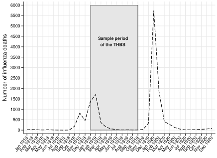
Figure 5: Number of Influenza Deaths in Tokyo between 1918 and 1920

Notes: This figure shows the time-series plots of the monthly death counts from influenza (ryūkōsei kanbō) in Tokyo prefecture between January 1918 and December 1920. The death statistics used in this figure were collected based on the comprehensive registration system.

Source: Created by the author using the 1918, 1919, and 1920 editions of the Statistics of Causes of Deaths of the Empire Japan (Statistics Bureau of the Cabinet 1921; 1922; 1923).

I begin my analysis by testing whether the illness of the head reduced the earnings. To do so, I decided the exact timing and duration of illnesses of the family members using the Kazoku idō hyō (Section 3.4). Figure 5 shows the number of monthly death counts from influenza (ryūkōsei kanbō) in Tokyo between 1918 and 1920. There appears to have been a moderate spike in early 1919, which is partially captured in the THBS period. In fact, a few THBS budget books suggest that the family members had caught the flu during this period. Five households experienced the illness during the sample period, and the illness affecting the heads was concentrated between February and May 1919, when the flu exposure was most prevalent. In addition, the average duration for the heads is $5.8$ days (Std. Dev. $=3.6$), which is consistent with the fact that Type A influenza causes fever for less than 6 days (Uyeki et al. 2022). Therefore, it is plausible to see that the influenza epidemics largely led to illnesses during this period. This historical event offers me a quasi-experimental setting in analyzing to what extent the adverse idiosyncratic shock driven by illness influences the households’ consumption behaviors.

Table 6 presents the results from the regressions of the head’s earnings on the number of days suffering illness in the previous semi-month cell. One must be careful that the head’s earnings in a specific semi-month cell depend mainly on the works in the last semi-month cell. In other words, if the health shocks have reduced their earnings, the lagged health shock has a clear effect on the earnings, whereas the instantaneous health shock has much smaller effects. Columns (1)–(3) confirms this mechanism. While the instantaneous health shock has little impact on the head’s earnings (Column 1), the lagged health shock has a statistically significant effect on his earnings (Column 2). This result is unchanged if I include both variables in the same regression in Column 3, supporting the evidence that the health shocks in the previous cell reduced the earnings of the head. The estimate in Column (2) suggests that a one-day increase in the illness decreases the head’s semi-monthly income by roughly $2.4$ yen. Notably, this is close to the average daily wage rate of skilled factory workers (Online Appendix B.6). Thus, this may reflect the reductions in their salary due to the absence. Finally, Column (4) adds the health shocks of the other family members into the specification of Column (3). The estimated coefficients on these placebo variables are statistically insignificant, supporting the robustness of the result in Column (3). These results confirm that the head who suffered illness lost earnings.

Table 6: Results of Testing the Impacts of Adverse Health Shocks
on the Head’s Earning

	Dependent Variable: Semi-monthly Earnings of the Head
	(1)	(2)	(3)	(4)
Health shocks on:
The head [level]	$-0.061$		$-0.972$	$-1.319*$
	$[0.679]$		$[0.699]$	$[0.666]$
The head [lag]		$-2.371***$	$-2.868***$	$-2.994***$
		$[0.644]$	$[0.734]$	$[0.765]$
The others [level]				$0.889$
				$[1.275]$
The others [lag]				$3.675$
				$[3.312]$
Observations	287	254	254	254

***, **, and * denote statistical significance at the 1%, 5%, and 10% levels, respectively. Standard errors in brackets are clustered at the household level.

Notes: This table shows the results from the regressions of the head’s earnings on the health shock variables using the semi-monthly panel dataset. A household with two semi-month observations is excluded from the sample in all the regressions because the lagged health shock variables are included. The family size variable, household fixed effects, and time-fixed effects are included in all the regressions. “Health shocks on the head” refers to the number of days that the head suffered illness. “Health shocks on the others” refers to the number of days that family members, excluding the head, were ill. “[level]” indicates the variable of the head’s earnings in the same semi-month cell. “[lag]” indicates the lagged variable (i.e., the shocks measured in the previous semi-month cell). Although correlation coefficient between the level and lag of the health shock variables for the other family members is substantially high (Pearson’s coefficient $=0.99$), including eather of the two variables does not change the finding on the neglisible impacts of the health shocks on the other family members.

Following the evidence, I characterize equation 1 as a structural consumption smoothing equation by using the first-stage reduced form equation as follows:

$$\log y_{i,t}=\beta h_{i,t-1}+\psi x_{i,t}+\varpi_{i}+\tau_{t}+e_{i,t},$$ (3)

where $h_{i,t-1}$ is the number of days of head’s illness in the previous semi-month cell, $\varpi_{i}$ is the household fixed effect, $\tau_{t}$ is the semi-month fixed effect, and $e_{i,t}$ is a random error term. For the risk-sharing mechanisms analysis under equation 2, the log-transformed disposable income in equation 3 ($y_{i,t}$) is replaced with the head’s earnings ($\tilde{y}_{i,t}$). The health shock variable is plausibly exogenous because the illnesses were from the influenza epidemics, as explained above. In addition, there is a correlation between the health shock variable and the head’s earnings at a statistically valid level (Table 6). Both support the evidence that the exogeneity of the instrument and relevance condition basically hold under this just-identified system.

Results: To what extent do illnesses affect consumption?

Table 7: Results of Estimating Income Elasticities:
Smoothing Consumption against the Adverse Health Shocks

	Semi-monthly Panel Dataset
	(1) Reduced-form approach			(2) Instrumental variable approach
	Head’s illness		Obs.	Disposable income		Obs.	First-stage
	Coef.	Std. error		Coef.	Std. error		$F$-statistics
Total consumption	-0.118	[0.015]***	254	0.543	[0.076]***	245	17.6
Food	-0.075	[0.017]***	236	0.355	[0.075]***	227	18.4
Housing	-0.017	[0.070]	126	0.118	[0.477]	126	7.6
Utilities	-0.051	[0.066]	199	0.201	[0.331]	192	12.4
Furniture	-0.157	[0.106]	156	0.761	[0.801]	150	6.2
Clothes	-0.339	[0.050]***	219	1.233	[0.222]***	211	65.4
Education	-0.099	[0.039]**	176	0.373	[0.153]**	170	45.9
Medical expenses	-0.002	[0.028]	236	-0.001	[0.142]	227	18.4
Entertainment expenses	0.019	[0.046]	224	-0.222	[0.501]	215	13.1
Transportation	-0.100	[0.094]	170	0.436	[0.510]	162	20.5
Gift	-0.325	[0.093]***	212	1.567	[0.797]*	204	17.8
Miscellaneous	-0.075	[0.027]***	195	0.343	[0.101]***	189	17.3

***, **, and * denote statistical significance at the 1%, 5%, and 10% levels, respectively. Standard errors in brackets are clustered at the household level.

Notes:

Column 1 shows the results of equation 1, in which the disposable income ($y_{i,t}$) is replaced with the head’s illness (i.e., the number of days with illness in the previous semi-month cell) as the idiosyncratic shock variable. The dependent variables are the 11 measures of log-transformed consumption, and all the regressions include the family size control, household fixed effects, and time fixed effects. The estimated coefficients on the health shock variable are listed in the column named “Coef.”.

Column 2 shows the results of equation 1, in which the disposable income ($y_{i,t}$) is regarded as the endogeneous variable. The head’s illness is an instrumental variable (i.e., excluded exogenous regressor) for the first-stage reduced-form equation. The estimated coefficients on the disposable income are listed in the column named “Coef.”. The first-stage $F$-statistics on the health shock variable are listed in the final column.

I first consider a reduced-form specification using the head’s illness as the exposure variable in equation 1 in the spirit of Cochrane (1991). Column 1 in Table 7 shows the results. Overall, the coefficients on the exposure variable are negative, supporting the evidence that adverse health shocks on the heads reduce consumption levels. The estimate for the food subcategories is smaller, as I found in my baseline result (Table 4). The estimate for the clothing category shows a relatively large magnitude, which is consistent with the adjustments in reducing luxury consumption. The expenses on gifts were also likely to be cut off in response to the adverse health shock as those are optional. Interestingly, the estimate for the education category is now statistically significantly negative. This may reflect the reduction of allowances for children in response to income losses due to health shocks.

Next, I explicitly model the structure behind the relationship between the health shocks and earnings using the reduced-form equation of 3. If the negative impacts of the health shocks on consumption were derived from the income losses, the results from this structural estimation approach are similar to those in Column (1). The estimates from the structural equation are listed in Column (2) of Table 7. The results are materially similar to the reduced-form results in Column (1), and the weak instrument issues are not relevant in most of the regressions. Overall, the estimates are systematically larger than those reported in Table 4. This partially reflects that the endogeneity is mitigated using the instrumental variable approach. It is important to remember that, however, this system intends to reduce the bias by specifying the channel from the adverse (instead of favorable) income shocks. In other words, I do not explicitly take the exogenous favorable shocks into account in the reduced-form equation. This would be another explanation for the difference in the results from my baseline results (Table 4). For example, expenses on the allowance for children could be easily cut during economic hardship but may not respond to favorable shocks. The expenses for furniture are also likely to be cut, but the households might not buy those frequently, meaning that there are no sufficient cases for reacting to the rare health shock events in my dataset. This may partly reflected in the smaller value of the first-stage $F$-statistics in the furniture subcategory. A similar interpretation can be applicable to the transportation category because the family travels did not happen frequently. While the estimates for clothes and gifts categories now exceed one, the null of equality to population mean of one are not rejected for both cases. Although the large estimates may partly due to the operation under the instrument based on the rare health shock events, the findings are materially similar to my baseline results: both categories are likely to be cut as those are dispensable categories.

Results: How did the households compensate for the losses from the ill?

Table 8: Results of Testing the Risk-Coping Mechanisms:
Adverse Health Shock as the Idiosyncratic Shock

	Semi-monthly Panels
	(1) Reduced-form approach			(2) Instrumental variable approach
	Head’s illness		Obs.	Head’s earning		Obs.
	Coef.	Std. error		Coef.	Std. error
Panel A: Savings, insurance, borrowing, and gifts (yen)
Net savings	0.397	[0.318]	254	-0.167	[0.117]	254
Net insurance	-0.168	[0.204]	254	0.071	[0.100]	254
Net borrowing	0.116	[0.261]	254	-0.049	[0.103]	254
Net credit purchase	1.294	[0.674]*	254	-0.546	[0.203]***	254
Net gifts	0.181	[0.177]	254	-0.077	[0.090]	254
Panel B: Labor supply adjustments & sales of miscellaneous assets (yen)
Other member’s earnings	0.001	[0.081]	254	-0.001	[0.034]	254
Sales of assets	0.002	[0.002]	254	-0.001	[0.001]	254

***, **, and * denote statistical significance at the 1%, 5%, and 10% levels, respectively. Standard errors in brackets are clustered at the household level.

Notes:

Column 1 shows the results of equation 2, in which the head’s earning ($\tilde{y}_{i,t}$) is replaced with the head’s illness (i.e., the number of days with illness in the previous semi-month cell) as the idiosyncratic shock variable. The family size control, household fixed effects, and time-fixed effects are included in all the regressions. The estimated coefficients on the head’s illness are listed in the “Coef.” columns.

Column 2 shows the results of equation 2, in which the head’s earning ($\tilde{y}_{i,t}$) is treated as the endogenous variable. The head’s illness is an instrumental variable (i.e., excluded exogenous regressor) in the first-stage reduced-form equation. The first-stage result is identical to the result listed in Column (2) of Table 6 with the first-stage $F$-statistics of $13.6$.

Panel A: Each net income variable is defined as the difference between income and expenses. “Net savings” refers to the difference between the amount withdrawn and the total deposits. “Net insurance” refers to the amount received from insurance minus the expenses paid for insurance. “Net borrowing” refers to the amount of borrowing minus the debt payments. “Net credit purchase” refers to the amount of credit purchases minus credit redeemed. “Net gifts” refer to the total received amounts, including both pecuniary and non-pecuniary gifts, minus the payments for gifts.

Panel B: “Other family member’s earnings” refers to the total income earned by all family members except for the head of the household. “Sales of assets” includes the sale of daily miscellaneous goods such as newspapers and empty bottles. All dependent variables are in yen.

I test the risk-coping strategies for mitigating adverse health shocks in Table 8. Column 1 lists the reduced-form results for the risk-coping strategies in the same manner in Table 5. The estimated coefficients on the net income variables are positive in most cases, suggesting the households’ compensating responses against the shocks. The estimate for the credit purchases category is weakly statistically significant, with the largest magnitude. It suggests that the one-day increase in the head’s illness increased the net credit purchases by $1.29$ yen, which accounts for roughly half of their average daily wages ($1.29/2.56$). Column 2 presents the estimates from the structural equation using the head’s earnings as the endogenous variable, which is instrumented by the head’s illness. A similar but much clearer result is obtained: the estimate for the credit purchases category is $-0.55$, which is roughly four times greater magnitude than that reported in Column (1) of Table 5. The estimate indicates that a one yen decrease in the head’s earnings increases the net income from credit purchases by $0.55$ yen. This magnitude is consistent with the direct effect of the health shocks on the net credit purchases estimated in Column (1) of Table 8. The estimates for the savings and gifts categories are still negative but now statistically insignificant, supporting the evidence that the credit purchase is the primary risk-coping strategy for dealing with the health shocks. Since it shall take more time (steps) from withdrawing and receiving gifts to use the money at the retailers, many households might prefer to use the credit purchases.

Overall, the event-study analysis using adverse health shocks confirms baseline findings and provides a sharper illustration of consumption smoothing behaviors in the case of adverse idiosyncratic shock events. In short, my results show that the unique available response among the THBS households to the idiosyncratic income shock was to use credit purchases. The available compensation via the credit purchases accounts for roughly half of their temporary income losses, which partially contributes to smoothing their food consumption in the short-run, say in a few weeks.

5 Credit System in Local Economy

Foregoing results shed new light on the roles of credit institutions among skilled workers’ households during historical industrialization. Since the credit purchases are provided by local retailers, this shows the importance of the relationships between the workers and retail shops. To the best of my knowledge, however, there is little historical work on credit purchases in prewar Japan. Therefore, the details of this credit institution are not yet clear: for example, how retailers get the credit information of their customers, whether the contracts are explicit or implicit, and whether the lenders enforce penalties for the debtors. The information on these institutions may be considerably personal, as in the case of state-contingent loans in the rural credit market (Udry 1994) and thus, are hardly be documented officially. In this section, therefore, I attempt to use the THBS dataset to investigate the institutions of credit purchases.

Table 9: Customers, Sales Methods, and Competitiveness in the Retailers in Tokyo City

Selling Item	Number of	Share of sales	Social Class of			Sales Method (%)			Number of
	stores	for regular	the Regular Customer (%)			Cash	Credit	Monthly	competitors
	reported	customer (%)	Upper	Middle	Other		purchase	installment	reported
White Rice	101	73.1	16	45.7	38.2	26.9	71.5	1.7	8.5
Fish	59	64.6	6.8	57.6	35.6	43.9	56.1	0	5.0
Greengrocer	66	45.4	9.4	40.4	50.2	65.8	34.2	0	6.2
Firewood and charcoal	100	51.1	15.7	50.9	33.4	20.4	78.4	1.3	8.6

Notes: This table summarizes the statistics on the sales in the $326$ retail shops selling white rice, fish, fruit and vegetables, and firewood and charcoal in Tokyo surveyed in 1935. The number of stores reported the share of regular customers (column 2) are $90$, $56$, $61$, and $93$ in the white rice, fish, greengrocer, and fuel (firewood and charcoal) categories, respectively. The share of regular customers is defined as the percentage of sales for regular customers in the annual total sales in 1935. The definition of the social classes (“Upper”; “Middle”; “Other”) is not exactly defined in the report. The share of sales method is based on the percentage of sales using each method in the annual total sales in 1935. The number of competitors indicates the number of peers within a three-cho, approximately $327$ meters, radius. The department stores and retail markets are not included in this survey.

Source: Tokyo City Chamber of Commerce and Industry 1937, pp. legend; 20–21; questionnaire.

Systematic information on credit purchases in the prewar period is unavailable. Fortunately, however, a survey report on retail shops in 1935 published by the Tokyo City Chamber of Commerce and Industry is remained. Table 9 summarizes the information on the sales in those retail shops of rice, fish, fruit and vegetables, and fuels. First, a large number of annual sales are from their regular customers, most of whom are from the non-upper classes. For example, $73$% of annual sales in rice retailers are from their regular customers, and more than $80$% of them are from non-upper classes, including the factory workers. Second, and most importantly, credit purchase is the popular sales method, especially among rice and fuel retailers: Evidence shows that more than $70$% of the sales were done with credit in both shops. Although cash was also used frequently among greengrocers, $34$% of the sales were settled using credit. This supports the evidence that credit purchases had been popular payment methods, and regular customers might settle a large part of them. Although these statistics are from the mid-1930s, this confirms the possibility that the retailers were engaged in credit transactions in the context of a long-term relationship with their customers. The final column of this table further provides suggestive evidence behind this. The survey asked retailers whether the sales area was competitive or not, and if yes, they were asked to report the number of competitors within a three-cho (roughly $330$ meters) radius. As shown, rice and fuel stores have 2-3 more competitors than the retailers selling fish, fruit, and vegetables. Given the relatively high utilization of credit in rice and fuel retailers, they may have responded to competition by allowing their customers to trade on credit.

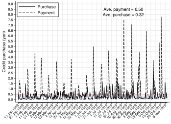
(a) Daily panel dataset:
purchase and payment

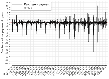
(b) Daily panel dataset:
net purchase

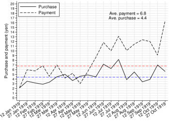
(c) Semi-monthly panel dataset:
purchase and payment

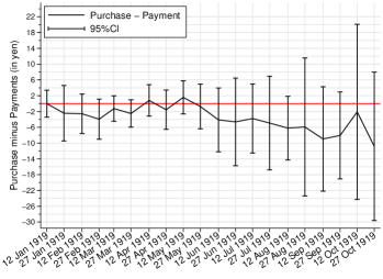
(d) Semi-monthly panel dataset:
net purchase

Figure 6: Relationships between Average Credit Purchases and Payments
by Different Time-series Frequencies

Note: Figure 6a, and 6c illustrate the time-series plots of the average daily and semi-monthly credit purchase and payment, respectively. Figure 6b and 6d illustrate the time-series plots of the average daily and semi-monthly credit purchase minus payment. Figures 6a and 6b show the daily data between 12th January and 11th November 1919. Figures 6c and 6d show the semi-monthly series calculated using the daily data between 12th January and 11th November 1919. All figures are based on the 30 THBS households that used any credit purchases.

Source: Created by the author using the THBS sample.

Next, I look into consumers’ credit purchase behavior using the THBS dataset. Most of the THBS households ($29/33$) used any credit purchases during their sample period, supporting the evidence that this was a common practice among the factory workers’ households in Tsukishima. Figure 6a illustrates the average credit purchases and payments based on the daily series. Generally, there is a peak per semi-month in payments, which reflects the households’ behavior of making the payments for the credit purchase on or soon after their paydays. The purchases series shows a similar tendency but with lower spikes and larger variance. This indicates that the households purchased goods by a certain amount around their paydays and then used it when they needed unconservable food such as fish, fruit, and vegetables. Figure 6b illustrating the net purchases confirms this behavior: while the households used the credit on a daily basis and redeemed near paydays. Figures 6a and 6d show that the average payment exceeds the average purchase in almost all semi-month cells, meaning that many households were able to repay their loans. This is consistent with the findings from the survey report that credit purchases function based on the long-term relationship between retailers and consumers in the local economy.

I then analyze whether the volatility of earnings restricts credit purchases. Since the credit of a worker is unobservable, I use the volatility of earnings as a proxy of credit risk in the following empirical specification:

$$I(\overline{CP}_{i}=0)=\varkappa_{0}+\varkappa_{1}CV_{i}+\bar{\mathbf{x}}_{i}^{\prime}\mathbf{\chi}+v_{i},$$ (4)

where $I(\cdot)$ is an indicator function, $\overline{CP}$ is the (unit-)average credit purchases, $CV$ is the coefficient of variation for head’s earnings, $\bar{\mathbf{x}}$ is a vector of the (unit-)average family composition variables, and $v$ is a random error term. All variables are calculated using the semi-monthly series. In this cross-sectional model, I include several family composition variables to control for unobservable preferences because the household-fixed effect is unable to be modeled as an error component. If retailers allowed households to use credit purchases regardless of the variability of earnings, the estimate of $\varkappa_{1}$ becomes close to zero. In contrast, if retailers did not allow households with high-income volatility to trade on credit, the estimate should be positive and reasonably large.

Table 10: Volatility of Earnings and Use of Credit Purchases

	Dependent Variable: Indicator Variable for
	Non-CP Users			Non-CP + Low-CP Users
	(1)	(2)	(3)	(4)	(5)	(6)
CV of Head’s Earnings	$0.003$	$-0.002$	$-0.027$	$0.019$	$0.008$	$-0.005$
	$[0.012]$	$[0.014]$	$[0.050]$	$[0.013]$	$[0.017]$	$[0.049]$
Sample mean of the DV	$0.12$	$0.12$	$0.12$	$0.24$	$0.24$	$0.24$
Model	LPM	LPM	Probit	LPM	LPM	Probit
Number of THBS households	33	33	33	33	34	33
Family Size	Yes	Yes	Yes	Yes	Yes	Yes
Children aged 6–12 (%)	Yes	Yes	Yes	Yes	Yes	Yes
Children aged 13–16 (%)	Yes	Yes	Yes	Yes	Yes	Yes
Adults aged 17+ (%)	Yes	Yes	Yes	Yes	Yes	Yes
Head’s age	No	Yes	Yes	No	Yes	Yes
Head’s earnings	No	Yes	Yes	No	Yes	Yes
Zero slope ($p$-value)	0.467	0.718	0.336	0.515	0.519	0.451

***, **, and * denote statistical significance at the 1%, 5%, and 10% levels, respectively. Robust standard errors are reported in brackets.

Notes: The dependent variable in Columns (1)-(3) is the indicator variable for the households who did not use any credit purchases during the sample period (non-CP users). The dependent variable in Columns (4)-(6) is the indicator variable for the non-CP users and households less than the first quartile in the sample average of credit purchases. The linear probability model (LPM) is used in Columns (1)-(2) and (4)-(5), whereas the Probit model is used in Columns (3) and (6). “CV of Head’s Earnings” indicates the coefficient of variations in the head’s semi-monthly earnings. The sample mean of the CV is $5.76$ (Std. Dev. = $5.72$). All the regressions include the family composition variables: average family size, share of children aged 6–12, share of children aged 13–16, and share of adults aged 17+ (share of children aged 0–5 is regarded as a reference). The average head’s age and average head’s earnings are added to the control variables in Columns 3 and 6. $F$-statistics $p$-values for the null of zero-slope hypothesis are reported in Columns (1)-(2) and (4)-(5). $\chi^{2}$-statistics $p$-values for the null of zero-slope hypothesis are listed in Columns (3) and (6). The standard errors for the LPM are based on the HC2 estimator proposed by Horn et al. (1975).

Column (1) of Table 10 presents the result for equation 4. The estimated coefficient is very close to zero and statistically insignificant. A potential concern herein may be the correlations between the volatility of earnings and the head’s age and earnings level. Column (2) shows the result from the extended model, including the head’s age and earnings, which shows the robustness of the baseline estimate in Column (1). Another potential issue is the functional form assumption in the LPM. Column (3) lists the result from the Probit model, including the full set of control variables used in Column (2), showing that the estimate is not statistically significantly different from zero. Next, I changed the threshold for the dependent indicator variable to consider a wider range of households using a relatively smaller amount of credit purchases, say less than the first quartile of the average credit purchases. Columns (4)-(5) summarize the results in the same column layouts as Columns (1)-(3), confirming that the estimates are still close to zero in all the specifications. Finally, the final row in this table shows that the null of the joint zero slope hypothesis is strongly rejected in all the regressions. Overall, there is no apparent trend in the characteristics of households to use credit purchases. This suggests that retailers may not have put weights on the volatility of earnings when trading with factory workers on credit. This is consistent with the retailers’ motivation to secure their local customers discussed earlier, and with the fact that factory workers commonly used credit purchases.

The results so far indicate that retailers have been generous in the earnings volatility risk. This, in turn, implies that retailers may factor risk in the form of interest into their loans or retail prices. Unfortunately, there are no systematic statistics on the interest in credit purchases. Thus, I calculate the risk premiums backward by differencing payments and purchases. This backward calculation technique requires information both on the price and type of retailers. However, budget books usually document price-by-item information but not price-by-retailer information. This is problematic because the same items were often sold in different types of retailers: for example, eggs were sold in greengrocers (yaoya) in many cases but sometimes sold in variety stores (aramonoya) too. Fortunately, I found that a specific month in a budget book has documented the price-by-retailer information. According to this budget book, the reimbursements were made semi-monthly, as seen in Figure 6b. They bought various goods in greengrocers, fish stores, and variety stores between 1st and 14th February 1919 and paid exactly the same amounts on the 15th. In the latter half of February, the household paid the same amounts to greengrocers and variety stores on 28th, but less amount to the fish stores. Since the budget book for March does not have information on the type of retailers, it is difficult to know exactly how the reimbursement shortfall was handled. However, this case suggests that the risk premiums may have been included in the retail prices but not in the form of interest.

To summarize, available documents suggest that retailers had to compete with other retailers in the same sales area and thus, provided consumers with the opportunity to trade on credit without interest for at least one month. This ease of accessibility to credit purchases might enable workers to smooth consumption in response to adverse idiosyncratic shocks in the short-run.

6 Conclusion

This study investigates the consumption behaviors among working-class households in Tokyo. I digitized the daily longitudinal budget survey on the factory worker households conducted in Tsukishima from 1918 to 1920 and implemented a systematic econometric method to obtain comparable estimates for income elasticities. The estimated income elasticity for total consumption indicates that the factory worker households suffered certain consumption losses when they faced idiosyncratic adverse income shocks. For consumption subcategories, I found evidence that while expenses on indispensable consumption categories are partially smoothed, expenses on dispensable categories are likely to be cut in response to the income losses.

The estimated elasticity for total expenditure ($0.55$) is in a similar range of those in rural eonomies in the developing countries, although only a few available references exist. According to Ravallion and Chaudhuri (1997), the elasticity for the rural households in Indian villages between 1975 and 1984 was roughly $0.5$. As for the urban hosueholds, the estimated elasticity is $0.4$ for Bangkok between 1975 and 1990, which had a similar GDP per capita to 1920 Japan (Townsend 1995). Since my estimate is from a specific occupation, skilled factory workers, one must be careful when making comparisons with estimates based on the samples including a variety of urban occuptions. At least, however, the factory workers in historical metropolis in Japan around the WWI had been relatively vlunerable against the idiosyncratic income shocks.

A recent study found an income elasticity of $0.39$ for factory workers’ households in Osaka city circa 1920 (Ogasawara 2024). My estimate from the adjusted monthly panels ($0.55$) is slightly larger than this estimate. Although the measurement errors in aggregate consumption and income in the monthly panel dataset may explain the discrepancy in these estimates, if taken literally, this implies that the Tsukishima factory workers were more vulnerable than those in Osaka. This indicates that higher levels of urbanization do not necessarily correspond to a greater availability of risk-mitigation institutions. Therefore, inter-city and cross-national comparisons of income elasticities and analysis of the institutional characteristics behind it will be the subject of future work.

My findings on the attenuation bias due to the measurement errors are potentially significant in that they may prompt a reinterpretation of the results obtained in previous studies. Errors in the timing of payroll can result in inconsistencies in the aggregate data for income and expenditure. An important point is that household-level studies often use aggregate data. In this case, modifying the aggregation period to align with wage payments can reduce attenuation. If the aggregation period cannot be changed, clarifying payroll timing and discussing potential bias is useful.

The results from mechanism analyses provide suggestive evidence that credit purchases played an important role in mitigating adverse idiosyncratic shocks to smooth food consumption. The institutional details of credit purchases should be investigated further. However, this finding offers a new historical view that interdependence between consumers and local retailers played a role in mitigating the idiosyncratic shocks on the workers. This implies that understanding the local retail system would be important in comprehending regional consumption behavior and, in turn, in understanding the improvement in living standards in prewar Japan.

Appendices

Appendix Appendix A Background Appendix

A.1 Developments of the Cities

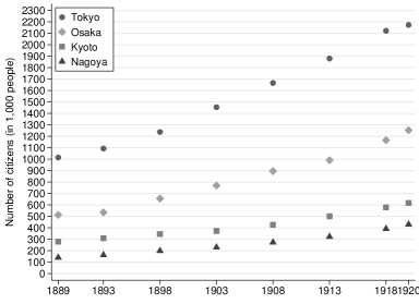
(a) Number of people in the large cities

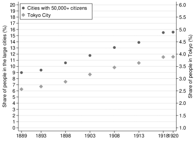
(b) Share of people in the large cities (%)

Figure A.1: Developments of the Large Cities in Japan

Note: This figure illustrates the development of large cities in Japan between 1889 and 1920. Figure A.1a shows the number of people in Tokyo, Osaka, Kyoto, and Nagoya. Figure A.1b shows the share of people in Tokyo (diamond) and the cities with more than $50,000$ people (circle) in total population in Japan.

Source: Umemura et al. (1983, pp. 303–305); Umemura et al. (1988, pp. 166; 168).

Table A.1: City Characteristics:
Tokyo, Osaka, Kyoto, and Nagoya

	Name of cities
	Tokyo	Osaka	Kyoto	Nagoya
Panel A: Population and Industrial Structures
Population	2,173,201	1,252,983	591,323	429,997
Male workers	768,633	476,229	189,922	138,275
Panel B: Industrial Structure (% share in male workers)
Agriculture	1.0	0.8	2.2	1.8
Fisheries	0.1	0.1	0.0	0.4
Mining	0.4	0.3	0.2	0.2
Manufacturing	44.5	45.6	49.0	45.8
Commerce	32.4	34.0	32.3	29.6
Transport	7.6	10.6	5.5	8.0
Public service and professions	11.3	6.7	9.0	11.3
Housework	0.3	1.8	0.1	0.0
Other industry	2.4	0.1	1.5	2.8
Panel C: Local Infrastructures
Number of electrical lights per people in 1921	0.9	0.8	0.9	0.9
Accessibility to modern water supply (%)	78.9	80.5	46.5	39.4
Panel D: Meteorological Features
January 1918 – December 1923
Average daily temperature	14.1	15.4	14.1	14.6
Average daily precipitation	4.7	3.9	4.6	4.8
February – April only
Average daily temperature	8.0	8.8	7.8	8.3
Average daily precipitation	4.2	3.4	4.1	4.3

Notes:

1. Panel A: The number of people and male workers measured in the Population Census conducted in October 1920 are listed.

2. Panel B: Occupations are classified based on the industrial classification of the 1920 population census. Unemployed people are not included in the calculation.

3. Panel C: The number of electrical lights measured at the end of 1921 is divided by the number of people in the 1920 population census. The number of houses accessible to water supply measured at the end of September 1920 is divided by the number of total households measured in the 1920 population census (%).

4. Panel D: The average daily temperature and precipitation between 1st January 1918 and 31st December 1923 and between 1st February 1920 and 30th April 1920 are listed.

Sources: The number of people in 1920 is from the 1920 Population Census (Statistics Bureau of the Cabinet 1928, pp. 186; 214; 222; 225). The number of male workers and their industrial structures are from the Statistics Bureau of the Cabinet (1929a, pp. 20–21; 26–29). The number of houses accessible to the water supply is from the Water Works Association (1922, pp. 69–70). The total number of households is from the 1920 Population Census (Statistics Bureau of the Cabinet 1928, pp. 186; 214; 222; 225). The number of electrical lights is from the Ministry of Posts and Telecommunications (1922, p. 558) The daily temperature and precipitation are from the Japan Meteorological Agency (database).

A.2 Financial Institutions in the Cities

Several financial institutions were available for working-class households in the cities around 1920.

A representative savings institution for households in prewar Japan is the postal savings (yūbin chokin). Although postal savings was initially designed as a small savings institution for low-income households, the share of postal savings to Japan’s total savings was roughly $10$% in the 1910s (Tanaka 2018, p. 29). The number of postal savings accounts per total population in the early 1910s exceeded $20$% in Japan (Tanaka 2018, p. 33), and the saving rate in prewar Japan was indeed higher than that of the U.S. (James and Suto 2011). As shown in Panel A of Table A.2, roughly $1.4$ million people had accounts in Tokyo in 1920, covering approximately $67$% of the entire population in Tokyo at that time. The average savings amount per capita was $64.5$ yen. The average figure for the postal savings accounts in Kyobashi Ward was $44.5$ yen at the end of 1919 (Tokyo City Office 1921, pp. 892–893). This amount is less than the monthly earnings of the skilled-factory workers (Section 3.2). Unfortunately, the statistics on postal savings by depositors’ occupation in Tokyo City are unavailable. However, this figure suggests that the average amount of postal savings was insufficient to smooth factory workers’ monthly consumption.

Savings bank (chochiku ginkō) is another famous savings institution for working-class households in the 1910s (Ito and Saito 2019, pp 79–81). Panel A of Table A.2 shows that the number of people having savings accounts was roughly $1.4$ million people had the accounts, accounting for approximately $58$% of total people in Tokyo at that time. Although this figure is similar to the postal savings, the workers in the manufacturing industry were less likely to rely on the savings banks than the workers in the other industrial sectors. Table A.3 summarizes the number of depositors and the amount of deposits by occupation in Tokyo City. In Kyobashi, the commerce and miscellaneous sectors shared roughly $84.8$% of all the depositors, whereas the manufacturing sector had only $11.5$%. This is mainly unchanged if I use the amounts of deposits to calculate the shares. Tokyo Institute for Municipal Research stated that this tendency captures the fact that savings banks are mainly designed as financial institutions for the lower-income class (Tokyo Institute for Municipal Research 1925b, p. 81). This suggests that skilled factory workers were less likely to use this savings institution. This may be consistent with the fact that Tsukishima did not have any savings bank branches, while there were two postal offices.

Mutual loan association (mujin) is another type of savings institution. The members of this association pay a fixed amount of money several times, and each member withdraws the total amount of payments each time under specific rules. The lotteries or bidding system decided which members could withdraw money each time. This means that the workers were less likely to use this institution to deal with the acute negative income shocks. Instead, it had been used to make a certain amount of money among small business owners and merchants. A report suggests that the workers in the manufacturing sector were roughly 10% of all the mutual loan associations in Tokyo (Tokyo City Office 1935, p. 25). Tokyo Chamber of Commerce stated that the mutual loan association was used for business and rarely used for household consumption (Tokyo Chamber of Commerce 1918, p. 121).

Cooperative societies were also available for worker households. Cooperative societies in Tokyo used credit as their payment method: households could buy goods in advance and pay at the end of the month or twice (middle and the end of) a month. The commodity prices were similar to or slightly lower than those in the retail shops (Central Federation of Industrial Associations 1925, pp. 18–19). However, the cooperatives only covered a few citizens. There were 26 cooperative societies in Tokyo prefecture in 1924, and 23 of them were organized by the citizens and workers (Central Federation of Industrial Associations 1925, p. 57–59). Among these 23 cooperatives, while the two largest societies had roughly 4000 members in total, the others were generally small societies with less than 100 members. This figure accounts for only a few percentage points in the workers in the city, given that the number of male workers was more than 768 thousand (Table A.1). Most of the THBS households had not used the cooperatives.

An alternative institution is the credit purchase in retail shops. The THBS households had often used the credit purchase in various retail shops for rice, fish, vegetables, alcohol, firewood, and charcoal. The details of the credit purchase are not described in the documents, and the systematic statistics on the credit purchase are also unavailable. This may be mainly because these transactions were conducted between each shop and worker. However, at least, the THBS budget data suggest that credit purchases had been widely used among the skilled-factory worker households at that time.

Pawnshops were the most popular lending institution among low-income working-class households. Lenders did not need to screen the borrower’s credit, and the borrowers did not worry about incurring heavy debt as the primary articles were inexpensive clothes (Shibuya et al. 1982). In addition, the interest rates were regulated by the Pawnbroker Regulation Act of 1895, and the average redemption rate was substantially high under the lower interest rates. Among $88$ pawnshops in Kyobashi, the average redemption rate was approximately $94$% ($401,222$ cases/$427,265$ cases) in 1920 (Tokyo City Office 1922b, pp. 888–889). The accessibilities were higher than the other lending institutions. The number of pawnshops in Tokyo was $1,334$ in 1918 and $1,261$ in 1919, respectively. The total number of cases was $8,226,883$ and $7,573,406$ each year. These figures are more than three times greater than the entire population in Tokyo City. As described in the main text, there were 13 pawnshops and only five moneylenders in Tsukishima. Thus, the accessibility to a pawnshop was undoubtedly high for the workers in the city.

However, the inexpensive article means that pawnshops were used to deal with very short-run necessities only. Among the pawnshops of Kyobashi, for example, the average amount per case was $7.8$ yen, which was $14$% of the monthly earnings of the THBS households. While the pawnshops were the popular lending institution, they could not offer a sufficient amount of temporary income for relatively large idiosyncratic shocks. According to the statistics on the pawnshop users in Tokyo prefecture in 1923, the share of agriculture, commerce, and manufacturing sectors were 1.7, 19.5, and 15.6%, respectively. The most representative users were the day laborers and workers classified as “miscellaneous”, accounting for $63.4$% (Tokyo Institute for Municipal Research 1926, p. 25). Tokyo City Office stated that the pawnshops were mainly used among low-income (poor) working-class households (Tokyo City Social Affairs Bureau 1921, p. 9). This indicates the evidence that the primary pawnshop users were not the skilled-worker households like the THBS households.

Another lending institution is the money lenders (kinsen kashitsuke gyō). Generally, business owners use money lenders, and the interest rates in the money lenders were very high compared with those in the pawnshops (Shibuya 2000, pp. 184; 248). Tokyo Institute for Municipal Research was concerned about the increasing number of unscrupulous companies arrested by the National Police Agency (Tokyo Institute for Municipal Research 1925b, pp. 106–108). Given this, while there were two money lenders in Tsukishima, they might have been less likely used by the factory worker households.

Credit unions (shinyō kumiai) are another institution available for working-class households. In Tokyo City, there were 215 unions in 1923. According to the survey of the 184 unions among them, however, the number of union members in the manufacturing sector was only $5,662$ (Tokyo Institute for Municipal Research 1925c, p. 20). This accounts for, at the most, only a few percentage points of the male workers in the manufacturing sector in Tokyo measured in the population census of 1920 (Online Appendix Table A.1).

Table A.2: Financial Institutions in Tokyo, Osaka, Kyoto, and Nagoya Cities in 1920

	Name of cities
	Tokyo	Osaka	Kyoto	Nagoya
Panel A: Savings Institutions
Postal saving
Number of depositors	1,462,604	725,642	305,927	172,183
Population percentage (%)	67.3	57.9	51.74	40.04
Total amounts (yen)	94,330,789	34,742,000	12,036,439	9,540,725
Amount per people (yen)	64.50	47.88	39.34	55.41
Savings bank
Number of depositors	1,461,389	1,648,090	663,831	482,960
Population percentage (%)	67.25	131.53	112.26	112.32
Total amounts (yen)	48,682,260	50,674,000	28,495,407	24,014,781
Amount per people (yen)	33.31	30.75	42.93	49.72
Panel B: Pawnshop
Number of shops	1,253	867	441	412†
Number of units lent	6,042,501	2,027,690	1,251,283	319,609
Amount of loans (yen)	38,667,993	3,785,186	4,424,357	2,983,250
Amount per loan (yen)	6.40	1.87	3.54	9.33

Notes:

1. Panel A: The statistics on postal savings were measured at the end of March 1921. The statistics on savings banks were measured at the end of 1920.

2. Panel B: Pawnshops in Tokyo, Osaka, and Kyoto were measured in 1920. Those for Nagoya (suggested in ${\dagger}$) were measured in 1923 because the statistics in the former years are unavailable.

Sources: Panel A: Tokyo City Office (1923, pp. 969; 977); Osaka City Office (1922, pp. 6(61); 6(67)); Kyoto Prefecture (1922, p. 257); Kyoto City Office (1926, pp. 188); Nagoya City Office (1922, pp. 286; 290). Panel B: Tokyo City Office (1923, pp. 888–889); Osaka City Office (1922, pp. 6(68)–(69)); Kyoto City Office (1922, p. 191); Tokyo City Statistics Division (1926b, p. 12).

Table A.3: Deposits in the Savings Banks in Tokyo City by Occupations

	Occupations
	Agriculture	Commerce	Manufacturing	Miscellaneous	Total
Entire Tokyo City
Number of depositors	76210	550784	166498	619963	1413455
Amount of deposits	2002124	19112713	6663091	19809591	47587519
Number of depositors (%)	5.4	39.0	11.8	43.9	100.0
Amount of deposits (%)	4.2	40.2	14.0	41.6	100.0
Kyobahi ward
Number of depositors	3809	34665	11664	51481	101619
Amount of deposits	130781	1218081	450805	1696086	3495753
Number of depositors (%)	3.7	34.1	11.5	50.7	100.0
Amount of deposits (%)	3.7	34.8	12.9	48.5	100.0

Notes: This table summarizes the number of depositors and the amount of deposits in the savings banks in Tokyo City by occupation on 31st December 1919.

Source: Tokyo City Office (1922a, pp. 864–865).

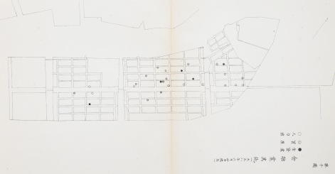
Figure A.2: Pawnshops and Money Lenders

Notes: This map shows the location of the pawnshops and money lenders in Tsukishima. Bullseye indicates the pawnshop (shichiya). The black circle shows the money lenders (kanekashi gyō). The white circle shows the rickshaw station (kuruma yado).

Source: Department of Health, Ministry of the Interior 1923c, tenth map. The tone was adjusted by the author using Adobe Photoshop 24.7.0.

A.3 Development of Tsukishima

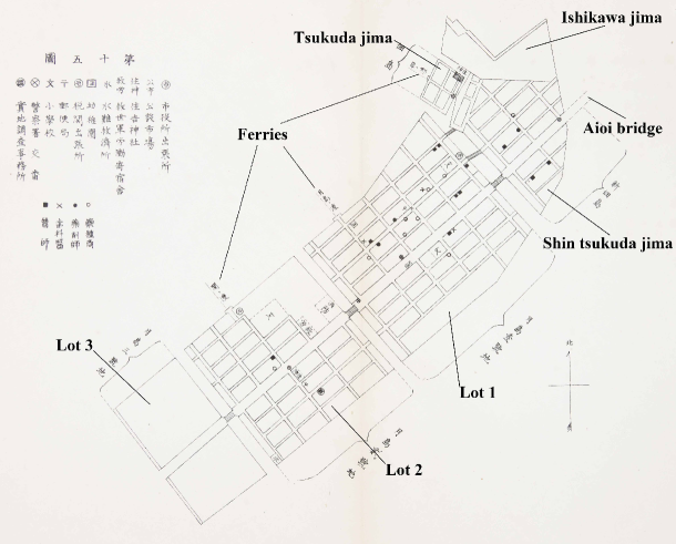
Figure A.3: Tsukishima: Ishikawajima, Tsukudajima, Shin-tsukudajima, and Lots 1–3

Notes: Tsukishima contains Ishikawajima, Tsukudajima, Shin-tsukudajima, and Tsukishima lots 1–3. This map does not illustrate the northernmost part of Ishikawa jima (see Figure 3 for this part). “Ferries” shows the Tsukishima to Kyobashi Ward sea routes: Tsukuda, Tsukishima, and Kachidoki routes (right to left). “Aioi bridge” links Shin tsukudajima and Fukagawa ward.

Source: Department of Health, Ministry of the Interior 1923c, 15th map. The author modified and adjusted the tone using Adobe Photoshop 24.7.0.

Tsukishima (transliterated as “moon island”) is a reclaimed land on a sandbar of the Sumida River. Ishikawa Island and Tsukuda Island at the northern end of Tsukishima are the starting point of its history. The following description of this section is based on Chūō Ward (1994, pp. 122–124).

Ishikawa Island was built in 1626 by a boatman, Hachizaemon Ishikawa, who received a fief from the Shogunate. In 1790, the Ishikawajima Prison was built on Ishikawa Island. This was a facility for the reintegration of minor offenders and those without lodgings and was called a Ninsoku Yoseba. After Perry arrived in Japan in 1853, the Shogunate ordered the Mito Clan to build a shipyard on Ishikawa Island. A month later, the groundbreaking ceremony was held for a Western-style wooden sailing ship delivered to the Shogunate in 1856. In 1866, the Ishikawajima Lighthouse was built on the west bank of the Yoseba and served to signal the position of ships entering the Nihonbashi direction. In 1870, the Ninsoku Yoseba became a place of imprisonment (Toba) and was renamed the Ishikawajima Jail Station of the Metropolitan Police Department in 1877. The prison was finally moved to Sugamo and the penitentiary on Ishikawa Island was closed in 1895.

Adjacent to Ishikawa Island is called Tsukuda Island, where fishermen from “Tsukuda” in Osaka Prefecture settled in 1644 after receiving land from the shogunate (the island was named after their hometown, Tsukuda). In 1645, the “Tsukuda ferry” began, and throughout the Edo period, Tsukuda Island was known as a fishing island for whitefish for the shogun’s household. In 1863, the Tsukudajima Battery was built on the south side of Tsukuda Island, one of 13 batteries used to defend Edo Bay. This battery later became the starting point for the reclamation of Lot 1 of Tsukishima.

In 1884, the Port of Tokyo Waterway Dredging Project was initiated. This was to secure the passage of ships by sweeping away the sediment in the shipping channel, and the Tsukishima landfill was created using the deposit. The first Tsukishima site was completed in 1891, and the “Tsukishima ferry” began the same year. The second site was created in 1894; then the Shin-(new) tsukudajima was built in 1896. From the west shore of Shin tsukudajima, the island overlooks the Boso Peninsula in Chiba Prefecture, making it a favorite vacation spot for writers. Cultural figures such as Toson Shimazaki and Kaoru Osanai stayed here from 1907 to the early Taisho period. In 1903, the Aioi Bridge was completed, bringing water and electricity to Tsukishima and improving transportation convenience, which contributed to industry development (until then, Suzukiiya had been selling water to supply the entire island using a ferryboat). The “Kachidoki Ferry” began to lead to Lot 2 in 1905. In 1913, Lot 3 was finally completed.

A.4 Housings in Tsukishima

Since the Tsukishima Survey included a housing survey (Table B.1), the type of housing in the entire island can be determined. Table A.4 summarizes the results of this survey. The description in this section is based on the Department of Health, Ministry of the Interior (1923a, pp. 69–76).

$88$ ($46$%) of the detached homes are in Tsukudajima. Tsukudajima is reported to be “superior to other areas in terms of housing quality, and the percentage of inferior housing is meager”. Conversely, Shin-tsukudajima has a low percentage of detached homes, is actually “inhabited by unskilled laborers” and “occupies the most inconvenient housing status of all the islands.” Lot 1 is a cluster of numerous residences, mainly tenements, which is consistent with the fact that Lot 1 functions as a center of life in Tsukishima. Lot 2 had a relatively high percentage of single-family and two-family houses and appears to have had a character as a “workers’ residential area” than Lot 1. These indicate that there may have been some geographic differences in income distribution regarding housing type.

Overall, however, of the $989$ dwellings in Tsukishima, $799$ ($81\%$) are row houses, and only $190$ are single-family homes. This confirms that Tsukishima was an industrial area with many working families. The workers lived in very similar tenements and with similar standards of living. Figure A.4 is a photo showing these tenement houses.

Table A.4: Housing Types in Tsukishima

		Tenement (nagaya)
	(A) Detached	(B) 2 families		3+ families		Total	(A)+(B)	%
		2-story	1-story	2-story	1-story
Tsukuda jima	88	32	26	6	23	175	146	83.4
Shin-tsukuda jima	16	27	10	36	59	148	53	35.8
Lot 1	58	62	74	73	200	467	194	41.5
Lot 2	28	27	43	9	92	199	98	49.2
Total	190	148	153	124	374	989	491	49.6

Note: This table summarizes the housing types in Tsukishima surveyed on 30th June 1919. Source: Department of Health, Ministry of the Interior 1923a, pp. 69–76.

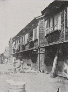
(a) 2-story tenement

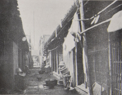
(b) 1-story tenement

Figure A.4: Photographs of the Tenements in Tsukishima

Note: Figures A.4a and A.4b show the two- and one-story tenements in Tsukishima, respectively. Source: Department of Health, Ministry of the Interior 1923c, figures 62–63; 66.

A.5 Machinery Factories in Tsukishima

First, I use the results of the Elementary School Children Survey included in the Tsukishima Survey to analyze the occupation (industry) of the head of the family household in Tsukishima. This is a survey of 4th-6th graders at Tsukishima 1st and 2nd Elementary Schools in July 1919. There were 1,173 children in the 3rd grade, and the survey included all 1,100 children who resided in Tsukishima. At that time, there were no other elementary schools besides those mentioned above. Thus, this survey is a complete survey for all children in grades 4-6 in Tsukishima. Although it does not cover households without children in grades 4-6, it is still a beneficial survey that provides an overview of the family households this paper covers. Panel A of Table A.5 shows the industrial structures. The composition ratios are similar to the census-based statistics shown in Panel A of Table 1. It does not specify whether brothers and sisters in the same household were counted twice. Despite this, this result confirms that the statistics obtained from this survey are useful in identifying overall trends in family households in Tsukishima.

Panel B of Table A.5 divides the “social classes” of the household heads in the industrial sector into six categories. The report considers large business owners to be the capitalist class, small business owners, free enterprise owners, directors to be the middle class, and workers to be the working class (Department of Health, Ministry of the Interior 1923a, p. 50). The table reveals at least three things. First, most heads of households in the industrial sector are workers, with only 1% of the capitalist class and less than 20% of the middle class. Although the definition of “executive” is unclear, it is unlikely that “small business owners” are households with a reasonably large income difference from skilled worker households because they must be small factory owners (Department of Health, Ministry of the Interior 1923a, p. 64).

Table A.5: Industrial Structure and Social Classes in Tsukishima

Panel A: Industrial Structure
Name of survey	Tsukishima Survey
Survey area	Tsukishima
Survey month and year	July 1919
Survey subject	Heads of all the students in grades 4–6
	in Tsukishima 1st and 2nd Primary Schools
	# of heads	% share
Agriculture	1	0.1
Fisheries	13	1.2
Mining	2	0.2
Manufacturing	623	58.6
Commerce	259	24.4
Transport	72	6.8
Public service and professions	55	5.2
Other industry	38	3.6
Observations	1,100	100
Panel B: Social Class of Heads in Manufacturing Sector
Name of survey	Tsukishima Survey
Survey area	Tsukishima
Survey month and year	July 1919
Survey subject	All students in grades 4–6
	in Tsukishima 1st and 2nd Primary Schools
	Tsukudajima	Shin-tsukudajima	Lot 1	Lot 2	Total
Large business owner	0	0	5	3	8
Small business owner	1	10	49	13	73
Self-employed	0	0	0	0	0
Executive	3	13	28	7	51
Worker	23	94	265	108	490
Unemployed/Unknown	0	0	0	0	0
Total	27	117	347	131	622
% share of workers	85.2	80.3	76.4	82.4	78.8

Notes: This table summarizes the statistics from the Complete Survey on the 4th-6th graders in Tsukishima1st and 2nd Elementary Schools in July 1919. Panel A summarizes the heads’ industries. Panel B sorted the “social classes” of the heads in the manufacturing sector. The report does not specify the definition of each “social class”.

Source: Department of Health, Ministry of the Interior 1923a, pp. 386–387.

In November 1920, there were 214 factories in Tsukishima, 168 of them (roughly $80$%) were classified as machinery factories. The official report documented that the wooden pattern factories could be included in the machinery sector because they were incorporated into the casting processes (Department of Health, Ministry of the Interior 1923a, p. 388). The share of machinery factories becomes approximately $90$% if I include those 24 wooden pattern factories.

Panel A of Table A.6 uses the manufacturing survey in the Tsukishima Survey to classify the 168 factories by size and industrial sector. First, more than $90$% of the plants are in the three sectors of machinery and equipment manufacturing, can manufacturing, and blacksmithing, with only $15$ plants in the casting sector. 113 ($67$%) of the machinery factories had workers less than 15. Second, many smithing factories have fewer than 15 workers. Hence, almost all of Tsukishima’s smithing industry was considered to be small businesses.

Panel B of Table A.6 classifies the types of the 620 workers based on the results of the primary school survey used in Table A.5. There were 455 skilled and 165 unskilled workers. Notably, these 620 workers include those not in the industrial sector: 490 industrial workers, 13 commercial, 61 in transportation, 16 in public service free trade, 38 in other gainful employment, and 2 in agriculture and mining in total. Since the workers in the industrial sector should include factory workers, workers in the cottage industry, and handicraft workers, the day laborers are considered to be classified into non-industrial workers (in fact, $620$ workers $-120$ day laborers $=490$). Therefore, it is estimated that roughly 90% of factory workers ($455/490$) were skilled workers, $65$% of whom worked in factories, $17$% in cottage industries, and $18$% as craftsmen. Since the workers in cottage and handicraft industries are considered to work in small factories, $65$% of these factory workers might had worked in the middle- to large-scale factories (with 15+ worerks).

One must be careful about the fact that this survey only covers the heads who had primary school children aged 9–11 (i.e., 4th to 6th grades), suggesting that most of these heads are in their 30s. Therefore, the share of skilled workers to the entire workers should be smaller than the $90$%. At least, however, it is plausible to see that almost all of the Tsukishima workers in their 30s were skilled workers at that time.

Table A.6: Scale of Machinery Factories and Type of Workers in Tsukishima

Panel A: Scale of Factories
Name of survey	Tsukishima Survey
Survey area	Tsukishima
Survey month and year	November 1920
Survey subject	All factories
	Machinery and	Drum	Casting	Smithing	Total
	equipment
# of workers $\geq 15$	22	15	10	8	55
# of workers $<15$	44	25	5	39	113
Total	66	40	15	47	168
Panel B: Type of Workers (All Industries)
Name of survey	Tsukishima Survey
Survey area	Tsukishima
Survey month and year	July 1919
Survey subject	All students in grades 4–6
	in Tsukishima 1st and 2nd Primary Schools
	Skilled workers			Unskilled workers
Factory workers	295		Factory workers	42
Cottage industry	76		Cottage industry	3
Handicraft industry	84		Day laborer	120
Total	455			165

Notes: Panel A summarizes the machinery factories by the scale of the factory. Statistics are from the manufacturing census conducted in the Tsukishima Survey (1st November 1920). The threshold (i.e., 15 workers) is based on the application of the Factory Act enacted in 1916.

Panel B sorted the heads by their skill level and job type. Statistics are obtained from the Complete Survey on the 4th-6th graders in Tsukishima1st and 2nd Elementary Schools in July 1919.

Source: Panel A: Department of Health, Ministry of the Interior 1923a, pp. 386–387; 410–414. Panel B: Department of Health, Ministry of the Interior 1923a, p. 149.

A.6 Works in the Machinery Factories

39% of the factories in Tsukishima are machinery and equipment manufacturing factories, the largest share of the machinery industry. Typical jobs for workers in machinery and equipment manufacturing plants are finishers (or fitters) and turners. A finisher is “a skilled worker responsible for finishing, assembling, and commissioning machine products” and is “one of the finest skilled workers because it requires skills in all aspects to correct defects in machine making” (p. 393). The turner is the “middle axis of machinists,” to which most semi-skilled and skilled workers belong. Becoming a full-fledged finisher and lathe operator takes at least five years. Generally, apprentices enter the workforce around 14–18, but they do not work in the same factory for many years within the apprenticeship system. After learning the skills for 1-2 years, they often move to another factory to improve their skills (p. 394).

Wages are paid on a piece-work basis or on a time basis. In Tsukishima, a time contract was adopted, and payment was based on the “residual time” method. Under the “residual time” method, “if the work is completed within the contracted time, the remaining time is considered the bonus.” For example, if 12 hours are contracted, and the work is completed in 10 hours, 2 hours are paid as a bonus (pp. 396-397). Wages were paid by dividing one month into two periods (first and second semester). The average workday in a machine shop is reported to be roughly 10 hours, with occasional all-night work (p. 402). Overtime hours were reportedly around 2 hours (p. 402).

Next, I summarize labor in the canning factory, which accounts for 24% of all Tsukishima factories. The can factory is said to be the “representative industry of Tsukishima”. It is said to be engaged in shipbuilding, bridges, steel frames for construction, and other works, including fabrication and repair of gas reservoirs (p. 406). Workers in a canning factory are called “boiler makers” and are typically involved in bending steel plates and joining them with rivets. Workers are divided into rivetter, holder-up, plater, angle-ironsmith, and caulking. The work is done in groups, with the skilled angle-ironsmith and caulking. The “bōsin” of the rivetter gives the instructions as the head of the group. Wages are paid on a piece-rate contract basis. Because of the contracted wage, the cannery workers’ income is unstable; thus, they are paid a fixed wage (daily wage amount) during the off-season.

Smithing is the second most common industry, accounting for 28% of the total. Panel A of Table A.6 reveals that most of the smithing industry is relatively small scale. They make boulders, nuts, rivets, lathe stops, jigs, and spanners for can manufacturing and construction. They were subcontractors who manufactured metal parts to supply the large factories on the island (p. 412). There were three types of jobs: yokoza, sakite, and tatara-fuki (bellows-blower). The yokoza were self-employed skilled workers (oyakata), while the other two were young unskilled laborers. In small operations, wages were based on a percentage based on voluntary business discussions with the proprietor, and working hours were not regular (pp. 411–413).

Appendix Appendix B Data Appendix

B.1 Tsukishima Survey: The First Social Survey in Japan

In modern Japan, the methodology of social research was formed in the 1930s. Before this, the generation of social research methodologies was attempted in the 1910s and 1920s (Kawai 1980, pp. 47–48). Kawai (1980, p.48) summarizes the history of social research methodology: during this period, “numerous social surveys were conducted by various survey entities, including government agencies, research groups, local administrative bodies, private organizations, survey research institutes, and researchers.” This is because “around WWI, there were many problems in labor, lifestyle, urban, health and sanitation, public safety, and civic due to the heavy and chemical industrialization, the monopolization of capitalism, and urban expansion”. The “Report on Field Survey in Tsukishima, Kyobashi Ward, Tokyo” (called Tsukishima Survey) used in this paper is the most pioneering of these surveys of urban communities. The Tsukishima Survey was a pioneering household survey in Japan (Sekiya 1970, p. 43).

First, I summarize the investigators, the research questions, and the subjects of the Tsukishima Survey. The person responsible for the Tsukishima Survey was Iwasaburō Takano (hereafter “Takano”), a professor of social statistics and social policy at the Law School of Tokyo Imperial University. Takano became a professor of economics at Tokyo Imperial University in 1919, and he became the director of the OISR in 1920. Takano placed great importance on gathering objective statistics about workers through social surveys (Sekiya 1970, p. 33). He had the experience of conducting the first household survey in Japan in 1916. Takano has been a member of the seventh subcommittee (Rural Sanitation Subcommittee) of the Ministry of Home Affairs’ Health and Sanitation Investigation Committee since 1916. In 1917, the Seventh Section evolved into the Section on Urban and Rural Sanitary Conditions (Kawai 1981a, pp. 12–13). On October 22, 1918, Takano submitted a proposal to the subcommittee for a field survey of urban sanitary conditions, which was approved. The survey aimed to determine the housing conditions, household budget status, and health status (child health, production, stillbirths, deaths, and diseases) in the areas where skilled-worker families congregated (Sekiya 1970, p. 6). Initially, the survey area was planned to be Yanagibashi Yokogawa-chō in Honjo Ward. However, at a committee meeting on November 23, the survey site was changed to Tsukishima in Kyobashi Ward, which had more skilled worker families than in Yokogawa-cho (Kawai 1980, pp. 55–59).

While the statistical method of sampling was not yet widespread at that time, Takano selected the survey sites based on his visionary thinking. In fact, “There can be no dispute that we have chosen Tokyo as the target of our metropolitan survey. However, it is impossible to survey the entire Tokyo area. We have no choice but to conduct a partial survey. For this purpose, it would be the best idea to select a representative area in Tokyo and survey that area narrowly but deeply.” (Department of Health, Ministry of the Interior 1923a, pp. 2–3). Takano further explained the need to focus on the working-class, which makes up most of the citizens, rather than the political and commercial center of Tokyo: “Most of Tokyo’s citizens are wage earners who subsist on labor. As is usual in large cities, a large number of people are engaged in manual labor in Tokyo. However, the most genuine type of worker is the skilled worker. Therefore, the area where many families of skilled workers congregate can be regarded as a representative area of Tokyo. And it seemed to me that a study of the social and sanitary conditions in that area could explain a large part of the social and sanitary conditions in Tokyo.” (Department of Health, Ministry of the Interior 1923a, pp. 3).

It is necessary to delve into the point where Takano states that “the most genuine type of worker is the skilled workers” and that the main target of the Tsukishima Survey was skilled workers. The description by Kawai (1981a, pp. 13–18) is helpful in this regard. As summarized in Section 2, Japan’s heavy and chemical industrialization throughout WWI led to a large concentration of city workers. As a result, the ratio of small-scale conventional factories based on “master employees” as is often observed in the textile industry decreased. On the other hand, the number of factories with a direct “factory owner-employee” employment relationship increased, particularly in the machinery and equipment, metal, and chemical industries. These workers in the modern industrial sector accumulated skills, formed households, and settled in the cities. It can be said that a new urban worker lifestyle was being formed. In short, although the city had a class of workers engaged in traditional industries, a new type of workers in the modern industrial sector, and a lower class, Takano believed that the skilled workers in the modern industrial sector would play a central role in terms of the labor force, labor movement, and urban life.

In addition, Sekiya notes the rise of the labor movement. As noted in Section 2, while wages rose throughout WWI, the price surge caused relative wages to decline. In 1916, Japan’s first labor protection legislation, the Factory Law, was enacted. However, the number of working days and hours did not decrease, and the number of labor disputes steadily increased (Sekiya 1970, pp. 24–26). Given this, Takano believed that workers should organize labor unions to help themselves with labor problems that could not be resolved through labor protection legislation. Sekiya (1970, pp. 26–40) speculates that Takano’s intention in conducting the Tsukishima Survey was to obtain basic data for solving labor problems, specifically to identify the scope of matters to be solved by workers on their own initiative (or covered by labor protection legislation). His insights suggest that this historical background must be addressed as a reason for Takano’s focus on skilled workers.

Kawai (1981b, pp. 15; 17) assessed the 40 households covered by the household survey included in the Tsukishima Survey as “the representativeness of the sample has remained ambiguous.” There is some mention but no clear description of how the sample households were characterized among the worker households in Tsukishima. It is reported that “to find suitable persons to fill in the form, we must ask for the assistance of school principals, police officers, physicians, and laborers, and we have requested a meeting of these persons at the survey office to explain the purpose of the survey, and to solicit applicants for the distribution of the household account book.” (Department of Health, Ministry of the Interior 1923a, pp. 8–9). As explained, the target households were not randomly selected because the statistical method of sampling was not prevalent (Section 3 provides a detailed analysis of the characteristics of the surveyed households). However, it is plausible that Takano designed this household budget survey in the sampling framework to capture the representative households in Tsukishima.

Table B.1: Survey Categories in the Field Study of Tsukishima Survey

	Periods of the	Chapter in the
	field studies	published report
1. Social mapping	Nov. 1918–May 1919	A2
2. Physical examination of children	Jan. 1919–July 1919	3
3. Physical examination of workers	June 1919	3
4. Nutrition survey of the worker households	May 1919	3
5. Survey of tenement houses	Autumn, 1919	3
6. Survey of sanitation occupation	June 1919	3
7. Sanitary survey in elementary schools	Unknown	3
8. Factory labor survey	Unknown	4
9. Labor household survey	Nov. 1918–Jan.1920	2
10. Elementary school survey	July 1919	2
11. Restaurant survey	Dec. 1919 & April 1920	2
12. Field survey of vaudeville	Dec. 1919	2
13. Survey of stalls and passersby	Dec. 1919	2
14. Photographing	Oct. 1920–Nov.1920	A2

Notes: The years/months listed in the first column (“Periods of the field studies”) are based on the description in the Department of Health, Ministry of the Interior (1923a, pp. 10–17). Figures listed in the second column (“Chapter in the published report” ) are based on the table of contents in the Department of Health, Ministry of the Interior (1923a, pp. 1–12; 1923b, pp.1–2). “A2” indicates the Appendix 2.

Sources: Department of Health, Ministry of the Interior (1923a, 1923b, 1923c).

Next, I overview the survey items and methodology. The investigation was primarily divided into “documentary” and “field” surveys. The former was an analysis of the characteristics of Tsukishima, using published statistics such as the census and the Police Department Statistics Book (Department of Health, Ministry of the Interior 1923a, p. 10). This was a pioneering attempt at the time and had influenced subsequent urban studies (Kawai 1980, pp. 61-62). The latter was a field survey including 14 survey items (Table B.1). It is not possible to describe all the survey items in detail, but following the report format described below, they can be divided into four large categories: 1. survey on workers’ livelihood (chapter 2); 2. survey on sanitary conditions (chapter 3); 3. survey on labor conditions in Tsukishima (chapter 4); and 4. social mapping and photography (appendix). The survey was conducted over two years, generally from November 1918 to November 1920, although the timing varied depending on the survey items (Table B.1).

A unique feature of the survey methodology is using young researchers as commissioned researchers. The household budget survey and leisure life survey were conducted by Gonda Yasunosuke, a faculty member of the Association for German Sciences “Doitsugaku kyōkai gakkō”, who had researched activity photography and entertainment. Tetsuo Hoshino, a medical doctor, was responsible for the sanitary survey. The labor survey was handled by Yoshitsuru Yamana, a graduate of Tokyo Imperial University who contributed to the organization of labor unions. In addition, Toyotaro Miyoshi, a sociology student at the Tokyo Imperial University, and others became temporary employees. In other words, although the Tsukishima Survey was initially planned as an insurance and sanitation survey by the Ministry of Home Affairs, in reality, it was a long-term survey conducted as a joint study by young researchers in different fields, led by Takano (Kawai 1980, p. 63). At the time, the Health Bureau of the Ministry of the Interior was conducting several sanitary surveys of rural areas. Takano might have designed the urban sanitary survey based on this background (Kawai 1981a, pp. 8–9). However, based on the idea that “health and sanitation surveys can at least encompass economic and social surveys,” Takano included a wide range of survey items, not limited to sanitation surveys (Department of Health, Ministry of the Interior 1923a, p. 56). Kawai (1980, p. 55) credits the Tsukishima Survey as a noteworthy pioneering concept: “going beyond a mere insurance and sanitation survey, it attempted to accurately depict the state of urban workers’ lives as they became established in the city during modernization, with skilled workers as its core.”

(a) Outside of the office

(b) Inside of the office

Figure B.1: Photographs of the Survey Office in Tsukishima

Note: Figures B.1a and B.1b show the outside and inside of the survey office in Tsukishima, respectively. Source: Department of Health, Ministry of the Interior 1923a, figures 1 and 2.

Takano stated, “To be as complete as possible, it is best to continue the survey over as long a period as possible and to obtain accurate facts by recording the workers’ household income and expenditures over a long period.” For this reason, he believed that “the best method of investigation would be to establish a survey station directly in the survey area and to have a full-time investigator reside there as much as possible, familiarize himself with the area and the people, and conduct the field survey” (Department of Health, Ministry of the Interior 1923a, p. 4). In fact, through the mediation of the Tsukishima police station, a research station was rented at 9-3 Higashinakadori, Tsukishima, where Yoshitsuru Yamana moved in from November 1918 and conducted contact with worker households (Department of Health, Ministry of the Interior 1923a, p. 7; Takeda 2015, p. 77). The survey office was open from November 1918 to December 1920, including the entire survey period (Figure B.1 shows the survey office).

It is also important to note that Takano and his team held weekly meetings at the research center during the survey period. Miyoshi recalls the situation at that time as follows:

After the start of the research station, all the members gathered once a week with Iwasaburo Takano present to discuss the implementation and progress of the survey and administrative matters. Iwasaburo Takano would always attend each meeting, happily listening to the results of the week’s research, inspecting the materials, providing detailed and thoughtful guidance, and usually ending the study session in a friendly atmosphere. Even now, I can recall the warm face of sensei (i.e., Professor Takano) of those days. It was always a friendly, laboratory-like atmosphere in which the C. Booth and S. Rowntree investigations were occasionally discussed.
Miyoshi (1980, p. 38)

He also states the following about Takano:

When the Tsukishima Survey was launched, the Faculty of Economics (in the Tokyo Imperial University) was becoming independent, and he was swamped both inside and outside the university. However, his enthusiasm for the Tsukishima Survey was extreme, and he was always present on his business trips to Tsukishima. Moreover, he made every effort to carry out his duties with precision.
Miyoshi (1980, p. 40)

Kawai (1981b, p. 28) assessed that there were no interconnections among the survey items mentioned above and that the survey “ended up being several fragmentary surveys rather than a comprehensive and systematic survey of workers’ lives.” The Tsukishima Survey is complex for secondary analysis because the sample size is small, and the statistics obtained through the study are not systematically compiled. This difficulty may be why previous studies have not frequently used the Tsukishima Survey. However, as already explained, Takano did not intend to conduct a large-scale social survey in Tsukishima in the first place. Instead, as he noted, the best method is to investigate a representative area “narrowly but deeply,” the goal was to improve the quality of the investigation rather than the scale of it. In this light, the fact that the researcher lived in the survey area and was constantly organizing and revising the survey results should be appreciated. Even though the Tsukishima Survey is the early social survey in Japan, it is of high quality as a prewar household survey.

Figure B.2: Official Published Report of the Tsukishima Survey

Notes: This photograph shows an example of the official report of the Tsukishima Survey published by the Department of Health, Ministry of the Interior, in 1923.

Source: Department of Health, Ministry of the Interior 1923b, title page. The tone was adjusted by the author using Adobe Photoshop 24.7.0.

Finally, I summarize the format of the report of the findings and the unpublished materials this paper will use. The results of the Tsukishima Survey were officially summarized in one report published in December 1921 by the Sanitary Bureau of the Ministry of the Interior and in two appendices (Figure B.2 is an example). The report was published under the name “Report on Field Survey in Tsukishima, Kyobashi, Tokyo,” and consists of four sections. The first section is a comprehensive review by Takano and outlines the survey. The second section summarizes the living conditions of the workers and was written by Gonda (partly by Yamana). Hoshino wrote the third section and summarized the sanitary conditions of workers. In the fourth section, Yamana summarizes the labor situation in Tsukishima. As for the two appendices, one contains statistical tables related to the above report, and the other organizes social maps and photographs. The correspondence between the survey items and the report is summarized in Table B.1. The Ministry of Home Affairs has already published these materials, which are available at the Gonda Yasunosuke Library of the OISR and the University of Tokyo Library.

B.2 Original Micro-spreadsheets from the Household Budget Survey in Tsukishima Survey

To analyze the consumption behavior of working households in detail, it is necessary to use the original individual survey forms. Unfortunately, the official report does not include individual data on the survey subjects, and many of the original forms used to prepare the report have yet to survive. However, some of the original slips are kept in the archives of the OISR because Takano was the first director of the OISR. The data used in this study to analyze household consumption are the individual data from the household survey (No. 9 in Table B.1), which Gonda used in writing the second section of the official report. While they have yet to be publicly available, I received permission from the OISR to use the original forms stored in the archives: the OISR, Archives of the Tsukishima Survey (THBS, unreleased).

Figure B.3: An Example Page of the Account of Household Expenses in the Tsukishima Household Budget Survey

Notes: This photograph depicts an example page from the household expenses account of the THBS. The right page documents the details of costs. The left page includes the details of revenue and receiving and making payments on the goods (actual things, including gifts).

Source: The THBS, account #6, 15th February 1919. The tone was adjusted by the author using Adobe Photoshop 24.7.0.

The household budget book used for the household budget survey in the Tsukishima Survey is named the Kinsendeiri hikaechō (money receipts and disbursements account book). This budget book is designed based on the form used in Takano’s first household survey (Online Appendix B.1) (Department of Health, Ministry of the Interior 1923a, p. 152). The budget book is to be filled out daily and includes four sections: income, expenses, receipts from credit purchases, and receipts and disbursements of actual goods. Most of the entries are in the income and expenses sections, indicating that living was basically conducted through wage receipt and consumption in cash. Figure B.3 shows an example of the budget book.

The method used to select households for the survey was not recorded in detail. According to the report, they initially recruited just over 90 households through the factory, police station, and elementary school in Tsukishima. Of these, 50 households completed the book for at least one month, but 10 were deemed incomplete and not included in the report. In addition to the 40 budget books used in preparing the report, therefore, the OISR has a set of other budget books marked as “discarded”. According to my survey, about six incomplete books of the worker households have been determined to be in this “discarded” category. Therefore, based on the remaining conditions of the books, it is plausible to believe that roughly 50 households participated in the survey. Of the 40 households included in the report tally, two households had recorded for more than one year, 11 households had recorded for 6–12 months, and the remaining 27 households had registered for less than six months (Department of Health, Ministry of the Interior 1923a, pp. 152– 153). Initially, the survey period was targeted to be six months, but the average bookkeeping period for the 40 households was four months.

B.3 Trimming

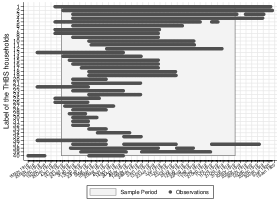
(a) Daily panel dataset

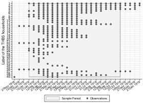
(b) Semi-monthly panel dataset

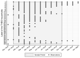
(c) Adj. monthly panel dataset

Figure B.4: Structures of the THBS Datasets by Different Time Frequencies

Note: Figure B.4a, B.4b, and B.4c show the observations in the daily, semi-monthly, and adjusted monthly panel datasets, respectively. For example, a marker in Figure B.4a indicates an observation in a specific year-month-date cell. Strictly, semi-monthly, and monthly datasets include both panel and cross-sectional units because aggregation shall trim fractions in the edges of the survey period. Figure B.4b shows 35-panel units and 5 cross-sectional units (#29; #31-33; #35). Figure B.4c also shows 35-panel units and 5 cross-sectional units (#29; #31-33;#35).

Source: Created by the author using the THBS sample.

In order to check whether the statistics from 40 THBS budget books contained any missing information, I digitized all 40 household budget books. Throughout this digitization process, I found that there are a few misreporting issues in the budget books.

First, there is a household that does not include information on income (household #37). Although the official report by Gonda reported the average monthly income for this household (Department of Health, Ministry of the Interior 1923a, p. 183), there was no documentation that would allow me to know how this average income was calculated. In order to avoid measurement errors in the income data, I excluded this household’s budget book. Similarly, a household does not include information on the payments to the credit purchases (household #39). Although the budget book of this household documented the amount purchased in credit purchases, I excluded this household’s book because the expenditure series becomes systematically smaller due to the omission of the payment information.

Second, the final pages of the budget books are sometimes omitted. This may be because the vendor who bound the budget books accidentally truncated the last page. All these incomplete sheets can not be included in the analysis.

Thrid, several households did not complete their budget books in the first and/or last month of the survey period. For example, the budget book of household #1 has statistics from 1st January 1919 to 12th January 1920. Similarly, the book of household #29 contains statistics from 26th January to 23rd February 1919. In semi-monthly and monthly datasets, these censored budget books may not be included in the aggregation. In the latter case, for instance, the budget sheets of 26th January and after 11th February 1919 are not included in a semi-month cell because the semi-month cell is defined from the 27th to 11th of the next month in this case. Thus, household #29 only has a cross-sectional observation and can not be included in the panel analysis.

Figure B.4 summarizes the structure of the 40 THBS households. Figure B.4a, B.4b, and B.4c shows the observations in the daily, semi-monthly, and adjusted monthly datasets, respectively. As explained, there are five cross-sectional units (#29; #31-33; #35) in the semi-monthly and adjusted monthly datasets. Therefore, there are 35 units with panel structure. After excluding a unit that does not have complete information on income (#37), I get the 34 THBS households as the analytical sample for my panel data analysis.

Regarding the time dimension, I trim all the observations before 12th January 1919 and after 11th November 1919 because the number of surveyed households is substantially small. For example, Figure B.4b shows that the number of cross-sectional units is three or less in both periods, causing substantial fluctuations in the net income. Consequently, my analytical sample includes 34 households measured between 12th January and 11th November 1919. The average number of semi-months per unit is $8.8$ (Std. Dev. $=5.0$). The characteristics of the 34 THBS households are summarized in detail in Section 3.

B.4 Testing the Potential Influence of the Unbalancedness

Table B.2: Results for the Balancing Tests

	DV: Indicator variable for the households
	with shorter time-series observations
	Threshold:
	(1) Median	(2) 75 percentile	(3) 25percentile
	($150$ days)	($184$ days)	($79$ days)
Size	-0.243	0.238	-0.135
	[0.244]	[0.254]	[0.294]
Children aged 6–12 (%)	0.017	-0.011	0.026
	[0.020]	[0.019]	[0.022]
Children aged 13–16 (%)	0.029	-0.050	0.057
	[0.038]	[0.045]	[0.041]
Men aged 17+ (%)	-0.008	0.008	-0.010
	[0.019]	[0.018]	[0.026]
Intercept	1.149	-0.576	-0.164
	[2.107]	[2.048]	[2.805]
Zero slope ($p$-value)	0.710	0.753	0.160
Maximized Log-likelihood	-21.8	-18.5	-15.2
Pseudo $R$-squared	0.046	0.046	0.171
Number of households	33	33	33

The results from Probit models are reported. Robust standard errors are in brackets.

Notes: The dependent variable is an indicator variable that takes one if the household has shorter time-series observations. Column 1 uses the median of the number of days per unit as the threshold. The result from the regression using the average number of days per unit ($144$ days) as the threshold is identical to that listed in column 1. Column 2 uses the 75 percentile of the number of days per unit as the threshold. Column 3 uses the 25 percentile of the number of days per unit as the threshold. All family size variables are the time-series average in each unit over the sample period. The proportion of children aged 0–5 years (%) is used as the reference group. Wald $\chi^{2}$ statistics $p$-values for the null of the zero-slope hypothesis are reported in the sixth row. The results from the expanded regressions including the head’s age and earnings are materially similar and the null of the zero-slope hypothesis is not rejected at the conventional level in all the specifications (not reported).

The unbalancedness in the THBS sample suggests that the attrition in several units may lead to selection bias in the sample. If the difference in the preference for consumptions predicted the large attritions, there must be statistically significant correlations between the family size variables and attritions. In other words, the units with shorter (longer) time-series observations have different preferences from those with longer (shorter). Table B.2 summarizes the results of the balancing tests for the 33 THBS households used in the analyses (Section 3.2). The dependent variable is an indicator variable that takes one if the household has time-series observations less than the median (column 1), 75 percentile (column 2), and 25 percentile (column 3). In Column 1, all the estimated coefficients on the family size variables are very close to zero and statistically insignificant, and the Wald statistics suggest the null results. This result is unchanged if I use the third and first quantiles in columns (2) and (3), respectively. Therefore, the family characteristics are similar in a statistical sense between the households with short-term observations and those with long-term observations. This supports the evidence that the unbalancedness in my THBS household panel datasets is not problematic in estimating their consumption behaviors.

B.5 Comparing Distributions of the Household Size

Figure B.5 illustrates the household size distribution measured in the census and THBS sample. The THBS does not include households with one person and with a large number of people (i.e., 9+). The number of households in the former class is $362$, accounting for only $6$% of the total number of households. The latter class has $294$ households, accounting for a smaller share with $5$%. Thus, the THBS sample covers most of the classes in the household sizes of Tsukishima. Although the THBS sample has a higher share of the category with four people than the census, the Pearson chi-squared test does not reject the null hypothesis of the equality of distributions with $p$-value of 0.948. This suggests that the THBS sample has a similar household size distribution to the population of Tsukishima (Section 3.1). It is, however, essential to remember that the THBS sample focuses on couples and households with children. This current study does not consider the consumption behaviors of the single factory workers’ households.

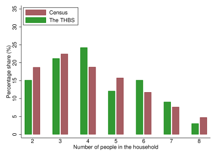
Figure B.5: Distribution of the Household Size:
Population Census v. the THBS sample

Notes: This figure shows the share of the household in each household size category to the total number of households in Tsukishima measured in the 1920 Population Census and the THBS samples. Pearson chi-squared test does not reject the null hypothesis of the equality of distributions with $p$-value of $0.948$. The share in each household size measured in the census is used as the theoretical probability in calculating $\chi^{2}$ test statistic (Pearson 1900).

Sources: Created by the author using the Tokyo City Office (1922a, pp. 262–283) and the THBS dataset.

B.6 Estimating Average Head’s Monthly Income

Comprehensive estimation effort on the time series figures of average wages in prewar Japan has been done in the Long-Term Economic Statistics. Specifically, the LTES estimates the average national salary series of “general occupations,” “manufacturing sector,” and “manufacturing occupations (by medium classification).” For the manufacturing occupations category, the average wage per day of factory workers in Tokyo City and Osaka city from 1917 to 1922 are reported (Ohkawa et al. 1967, p. 255). These values were estimated using the “Annual Statistics of the City of Tokyo” (hereafter, the ASCT) and “Osaka City Statistical Table.” However, the household survey includes the household head’s monthly income but no information on the daily wage. Hence, the “average daily wage per factory worker” estimated in the LTES cannot be directly compared to the monthly income of the head of household, which is obtained from the Tsukishima Survey. In this section, I use available wage and labor statistics to estimate the average monthly income of male factory worker households in Tokyo and compare it to the THBS heads’ average monthly earnings.

To clarify the problem, I estimate average monthly earnings most simply. Specifically, I use the ASCT (volume 17), which provides wage statistics as of the end of 1918, as a case study. The ASCT (Volume 17) provides the “average daily wage of male factory workers aged 15 and over,” “number of factory workers aged 15 and over,” and “average number of working days per year” by industrial sector for four categories of factories: factories with ten or fewer workers, and factories using or not using motive power. Using the “number of workers over 15 years old” obtained for each factory category cell in each industrial sector as weights, I can get, for example, the average wage per month for a worker in the machinery sector as:

$$\textit{Wage}^{15+}_{Machine}=\frac{\sum_{c}\{(\textit{Daily Wage}^{15+}_{Machine,c}\times\textit{Working Days}_{Machine,c})\times\textit{Workers}^{15+}_{Machine,c}\}}{12\sum_{c}\textit{Workers}^{15+}_{Machine,c}}.$$ (5)

This value is estimated at $27.8$ yen. This is the most straightforward estimate using daily wages, the number of workers, and the number of working days, and thus has several significant problems that create a downward bias in the estimates.

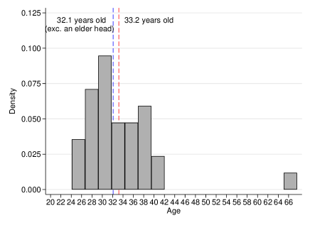
Figure B.6: Distribution of the THBS Heads’ Age

Notes: This figure shows the density of the THBS heads’ age calculated from the THBS daily panel dataset. The dashed line (red) indicates the average age of all the heads (33.2 years old). The dashed line (blue) shows the average age of the heads, excluding an elder head aged 67.6 (32.1 years old). The difference between the two average figures is statistically insignificant with $p=0.4087$.

Source: Created by the author using the THBS dataset.

The first issue is that the average wages of factory workers listed in the ASCT (volume 17) are summarized as “15 years old or older.” Figure B.6 shows the THBS heads’ age distribution. The mean value is $33.2$ years old, which is unchanged (i.e., $32.1$ years old) if I exclude a head aged more than $60$. Only nine heads are under 29 years old, and most are around 30 to early 40s. This means I have to refer to the average daily wage for the 30s to 40s. However, since the number of factory workers is concentrated in the 20s, the average wage reported in the ASCT shall be considerably lower than the average wage for factory workers around 30 years old. To correct for this downward bias, I need the wage profiles by age.

Second, there is no consideration of ancillary pay such as bonuses and various allowances. As explained later, these “accessory wages” were not negligible at the time. Thus, estimation without considering ancillary pay would have a non-negligible downward bias. In the following, I summarize the procedure for correcting such downward bias.

B.6.1 Daily Wage Distribution by Ages

Since the early wage surveys focused on average wages, official statistics in the 1910s do not include average wage statistics by age (bin). By the “Statistical Data Field Survey Law” (Law No. 52) in April 1922, average wages by age group were surveyed for the first time in the “Labor Statistics Field Survey” in October 1924 conducted by the Social Affairs Bureau of the Ministry of Home Affairs (Committee for the History of the Labor Movement 1964, p. 14). The official reports of this survey in Tokyo were summarized as the Labor Statistics Table (hereafter, LST) for Tokyo City and Suburbs and published by the Tokyo City Statistics Division in 1926.

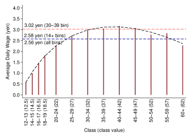
(a) 1918

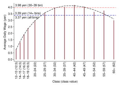
(b) 1919

Figure B.7: Daily Wage by Age Bins: 1924 Manufacturing Census

Notes: This figure shows the daily wage distribution by age bins measured in the manufacturing census in 1924. The weighted average daily wage for 30-39-year-old bin is shown in red. The weighted averages for all and 14+ bins are shown in gray and blue lines, respectively. The fitted fractional polynomial models are shown in the dashed lines. For the 1918 price data, the fitted model is $\hat{y}^{\textit{Daily Wage}}=-10.01+4.15a^{1/2}-0.33a^{2}$ with $R^{2}=0.99$. For the 1918 price data, the fitted model is $\hat{y}^{\textit{Daily Wage}}=-13.18+5.47a^{1/2}-0.43a^{2}$ with $R^{2}=0.99$.

Sources: Created by the author using the Tokyo City Statistics Division (1926a, pp. 16; 244-245). Data on the consumer price index for the cities are obtained from Ohkawa et al. (1967, p. 135).

Figure B.7 depicts daily wages by age for male factory workers in Tokyo City’s machinery and equipment manufacturing industry, based on statistics obtained from the LST. There are 13 age bins, and the number of workers and average wages are listed for each bin. Figure B.7a shows the distribution of wages adjusted to 1918 prices using the consumer price index (CPI) for urban areas (Ohkawa et al. 1967, p. 135). The weighted average for ages $14$ and older is $2.58$ yen, which is about the same as the weighted average for daily wages of $2.56$ yen. The $2.58$ yen is between the average values for the 20-24 age bin and the 25-29 age bin. Thus, it may represent the daily wage of workers around 25. This is consistent with the fact that workers are concentrated in the 20s. However, the weighted average for the 30-39 age bin is $3.02$yen, which deviates significantly from the weighted average. The distribution of wages at 1919 prices shows a similar result (Figure B.7b). Using weighted averages for earnings comparisons leads to the erroneous conclusion that the sample households are upwardly biased.

To address these issues, I use the following steps to estimate the distribution of wages of the factory workers in Tokyo City in 1918-1919, the observation period of the THBS sample. Since the same estimation method is used for both years, I use 1918 as an example below.

First, the distribution of daily wages by age group was projected from statistics obtained from the LST. Following Royston and Altman (1994), I consider a fractional polynomial of degree $m$ as follows:

$$\phi_{m}(a;\bm{\varphi},\mathbf{p})=\varphi_{0}+\sum_{j=1}^{m}\varphi_{j}a^{(p_{j})},$$ (6)

where $a$ ($>0$) denotes class value of age bin, $\bm{\varphi}$ is a vector of coefficients and $\mathbf{p}$ is a vector of powers, satisfying $p_{1}<p_{2}<...<p_{m}$. $a^{(p_{j})}$ indicates the Box-Tidwell transformation, taking $\text{ln}(a)$ if $p_{j}=0$ and $a^{p_{j}}$ if $p_{j}\neq 0$. As suggested in Royston and Altman (1994, p. 433), the models requiring a degree higher than two ($m>2$) are rare in practice. The wage by age bin distribution illustrated in Figure B.7 clearly shows a simple quadratic curve. Thus, I consider a fractional polynomial function with degree two as follows:

$$\phi_{2}(a;\varphi_{0},\varphi_{1},\varphi_{2},p_{1},p_{2})=\varphi_{0}+\varphi_{1}a^{(p_{1})}+\varphi_{2}a^{(p_{2})}.$$ (7)

To model the function, I consider a set of powers $\mathscr{P}=\{-2,-1,-0.5,0,0.5,1,2,3\}$ in the spirit of Royston and Altman (1994, p. 434).

The maximum likelihood estimation is used to search for the most suitable candidate of the coefficients for a given $m$. Since $m=2$, there are ${}_{8}\mathrm{H}_{2}$ ($=36$) repeated combinations for the candidates of the parameters. By adding the $8$ simple candidates under the nested models (i.e., the models with degree-1 fractional polynomial) to be conservative, I run $44$ regressions in total to find out the model with the highest maximized log-likelihood. The best power vector suggested is $(p_{1},p_{2})=(0.5,1)$. The projection model fitted using the best power vector is as follows:

$$\hat{y}^{\textit{Daily Wage}}=-10.01+4.15a^{\frac{1}{2}}-0.33a^{1},\quad R^{2}=0.99.$$ (8)

The dashed curve in Figure B.7 is the predicted distribution in equation 8. The precise fitting suggests that the predicted distribution works properly, especially below 50-54 bin.

Next, I shift the predicted distribution based on the difference in the average daily wages in the ASCT and LST. The weighted average of the daily wage is $2.56$ yen for the LST, whereas that for the ASTC is $1.05$ yen, meaning that there is roughly $1.5$ yen difference. Thus, I shift the functional polynomial function by this amount of difference to yield the proxy distribution for 1918. Figure B.8a illustrates this operation: dotted curve is a fractional polynomial shifted from the original fractional polynomial shown as a short dashed curve.

The average daily wage for 12–14-year-old bin is reported to be $0.42$ yen in the ASCT, whereas that for 12–13-year-old bin in the LST is $0.60$ yen. This difference (i.e., $0.18$ yen) is smaller than the difference in the weighted average for all age bins (i.e., $1.5$ yen). This implies that the daily wage by age distribution in the ASCT could be smoother (i.e., flatter) than that of the LST. Thus, the shifted fractional polynomial would provide stronger shrinkage for those bins of younger age. In other words, the shifted curve shall get closer to the actual (unobservable) wage distribution as age increases.

The long dashed curve in Figure B.8a examines this relationship by fitting another fractional polynomial model using the 12-14-year old bin figure of the ASCT and the predicted wages for 25–65 from the shifted fractional polynomial. Let this curve a predicted wage distribution for the true distribution. The average daily wage for the 30–40-year-old bin in the shifted fractional polynomial is $1.55$ yen, which is similar to that for the same-age bin in the predicted wage distribution (i.e., $1.52$ yen). However, the wage gaps for the younger ages show more significant differences. As long as our interest is in the late 20s to the early 40s, therefore, it is plausible to employ the predicted wages for the wage comparison conducted in Section 3.

Figure B.8b illustrates the result of the same analysis from the wage data of 1919 price, reflecting the increasing trend in price between 1918 and 1919. The average daily wage for a 30–40-year-old bin in the shifted fractional polynomial is $2.46$ yen. Again, this is similar to that for the predicted wage distribution (i.e., $2.42$ yen).

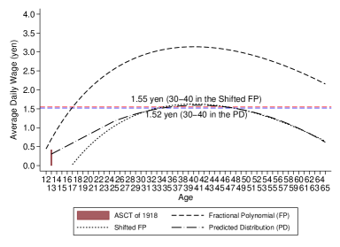
(a) 1918

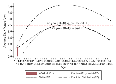
(b) 1919

Figure B.8: Daily Wage by Ages Distribution:
Shifted Fractional Polynomial

Notes: The short dashed curve illustrates the fractional polynomial (FP) in Figure B.7. The dotted curve indicates the FP shifted by the difference in the average daily wage between the ASCT and LST. The ASCT documents the wage statistics for four different categories for each manufacturing sector: the scale of the factory (10+ or below ten workers) and engines (use or not). I calculated the weighted average of the daily wage using the number of factory workers in each age bin and the category as weights. The long-dashed curve shows the FP refitted using the average daily wage for 12–14-year-old bin ($0.42$ yen) measured in the ASCT and the daily wages for 25–65-year-old suggested in the shifted FP. The average daily wage for a 12–14-year-old bin is only available for the ASCT of 1918. Therefore, this figure for the 1919 price is calculated using the ratio between the average daily wage ($1.05$ yen) and that for 12–14 years old bin ($0.42$) in 1918 as $1.80\times(0.42/1.05)$, where $1.80$ is the average daily wage measured in the ASCT of 1919. The red dashed line is the average daily wage for 30–40-year-old in the shifted FP. The blue dashed line is the average daily wage for 30–40-year-old in the refitted FP.

Sources: Created by the author using the Tokyo City Office (1921, pp. 726–757); Tokyo City Statistics Division (1926a, pp. 16; 244-245).

As I explained later, the average size of factories in Tsukishima was larger than in the entire city (Panel C in Table B.3). Since the larger factories had at least larger ancillary wages, the factory workers in Tsukishima might have had more earnings than those in the entire city (Online Appendix B.6.2). Therefore, it is important to remember that the average daily wages calculated in Figure B.8 are conservative estimates for the average daily wage for the skilled workers in the machinery sector in Tsukishima. However, given the scarcity in the wage-by-age statistics, I refer to these wages in the monthly wage calculation in Online Appendix B.6.3.

B.6.2 Ancillary Wage

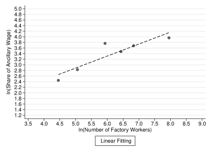
Figure B.9: Log-Relationship between the Number of Workers and Share of Ancillary Wage: Original Data from the Factory Survey by Kitazawa (1924)

Notes: This scatter plot shows the relationship between the log-transformed number of factory workers and the log-transformed share of ancillary wage. The raw data are listed in Table B.3. The dashed line indicates the linear fit using the log-transformed variables: the fitted regression is $\hat{y}=0.747+0.428x$ with $R^{2}=0.82$. The predictions are materially similar if I use the fractional polynomial using the raw data on the number of factory workers and share of ancillary wage in Table B.3. In the case of fitting based on the raw data, the fitted fractional polynomial model is $\hat{y}^{\textit{Daily Wage}}=53.6-399.3a^{-1/2}+(2.84\times 10^{-10})a^{3}$ with $R^{2}=0.87$. I prefer to use linear regression herein because it can provide more precise fitted values for factories with a small number of workers.

Source: Kitazawa (1924, pp. 20; 58–62).

The daily wage estimated in Section B.6.1 is a fixed salary and, thus, does not include additional salaries (bonuses and allowances). Some data on bonuses and allowances in prewar Japan are available for the pre-Showa period, but unfortunately, there are no systematic statistics (Committee for the History of the Labor Movement 1964, pp. 14–15). In this section, therefore, I use available data from a detailed survey of factory workers’ salaries to determine the percentage of wages outside of regular pay. In the following, wages other than regular salaries, such as bonuses and allowances, are collectively referred to as ancillary wages.

Since the Tsukishima Survey targets skilled worker households, knowing the ancillary wages paid to skilled workers is necessary. The “Wage Survey Report” by Kitazawa (1924) is helpful in this regard. This report includes the result of a survey on the wages for machine finishers (fitters) and turners at six machine factories in Tokyo from May–October 1921. This is particularly useful as it examines the wage structure of skilled factory workers.

There are two methods of paying wages to workers in the machine industry: one is to use hourly wages to calculate fixed salaries, and the other is to combine hourly wages with piece-rate wages, with the former being the most common (Kitazawa 1924, p. 33). However, wages paid in both methods are divided into fixed salaries and other ancillary wages, and there is not much difference in essence (Kitazawa 1924, p. 39). Fixed wages are salaries added from a fixed hourly wage rate, while ancillary wages include bonuses and overtime pay, night shift pay, and labor premiums (profit sharing). In the case of a combination of hourly and piece-rate pay systems, the accessory wage includes a share of the piece-rate profit.

Panel A in Table B.3 summarizes the survey results. The surveyed factories included 86, 157, 376, 623, 928, and 2,837 workers, ranging from small to large. The percentage of skilled workers (finishers and turners) in the surveyed factories ranged from $27$% to $77$%, and the portion of monthly ancillary wages was 12–53%. Figure B.9 is a linear regression fit using log-transformed data on the percentage of ancillary wages and the number of workers. There is a positive correlation between the factory size and ancillary wages. This is consistent with the historical fact that larger factories have more extensive benefits than smaller ones (Odaka 1999).

Next, I estimate the percentage of ancillary wages at the Tsukishima factories. One of the most frequently used statistics on factories in Tokyo is the Handbook of Factories (kōjyō tsūran), which covers all the factories with ten or more workers as of January 1, 1920. This handbook is the most comprehensive source for ascertaining the number of factories and their sizes around 1919. This document does not cover the number of tiny working places with less than nine workers. Importantly, however, the purpose of Panel C in Table 2 is to compare the average monthly wage of the skilled factory workers employed in the Tsukishima factories and the THBS heads’ average monthly earnings. Therefore, the censoring at the left tail of the factory size distribution is manageable for this purpose.

Columns 1 and 2 in Panel B of Table B.3 summarize the distributions of the number of factories, and the number of workers in Tsukishima reported in the handbook. Column 3 summarizes the average of the ancillary wage estimates predicted in Figure B.9. The average ancillary wage at the Tsukishima factory is about 12%, which is close to the value for the entire city of Tokyo (9%).

Panel C in Table B.3 compares the size of factories obtained from the handbook with the size of factories where the THBS heads in the machine industry worked. There are 32 (out of 40) heads of household for which the name of the factory where they worked is known. For 31 of these heads, the number of workers can be obtained from the handbook. In addition, three others are self-employed, two of whom are blacksmiths. Since these three were self-employed owners of tiny factories, I assume the number of workers to be 10, based on the report (Department of Health, Ministry of the Interior 1923a, p. 412). Column 1 of Panel C summarizes the distribution of plant sizes worked by these 35 heads of households. Compared to the distribution in Tokyo City and Tsukishima (columns 2–3), the THBS heads worked at the larger-scale factories.

Column 4 uses the same method as Panel B to calculate the average share of the ancillary wage for the THBS heads. The averages for the classes ranging from 10 to 199 workers are very similar to those of the THBS heads, Tsukishima, and Tokyo City classes. Despite the differences in the factory sizes, this supports the evidence that the THBS heads who worked in the small and medium-sized factories earned similar wage levels to the entire Tsukishima and Tokyo City.

However, in the 200+ bin, the average value of THBS heads (57%) is larger than the average value in Tokyo and Tsukishima (columns 3–4 in Panel B). This is because 13 heads of households work at Ishikawajima Shipyard, which has over 3,000 workers. Since there is a variation in the monthly earnings among the THBS heads working at the Ishikawajima Shipyard, the average value of THBS heads in the 200+ bin does not always represent the share of the ancillary wage for these heads. However, the percentage of workers in large factories is relatively higher in the THBS heads than in Tokyo City and Tsukishima. This suggests that these heads got a higher percentage of ancillary wages than the average. Therefore, the average monthly earnings of the THBS heads may be more or less higher than the average monthly income of the skilled workers in the Tsukishima factories.

Table B.3: Estimating the Average Share of Monthly Ancillary Wage

Panel A: Original Data on the Share of Ancillary Wage
Document: Report of Factory Survey by Kitazawa (1924)
Survey subject: Six Machinery Factories in Tokyo City
Survey month and year: May to October 1921
	Number of	Share of	Share of	Share of
	factory	skilled	fixed	ancillary
Factory	workers	workers (%)	wage (%)	wage (%)
A	157	44	83	17
B	86	53	88	12
C	376	27	57	43
D	623	77	68	32
E	2837	NA	47	53
F	928	41	60	40
Panel B: Estimating the Average Share of Ancillary Wage
Document: Handbook of Factories (1921 edition)
Survey subject: Machinery Factories with 10+ workers in Tokyo City
Survey month and year: January 1920
	Machinery Factories
	Tsukishima			Tokyo City
	(1) Number	(2) Average	(3) Average	(4) Average
	of factories	number of	share of	share of
Factory size		factory workers	ancillary wage (%)	ancillary wage (%)
Total	47	124	12	9
10–99 workers	39	32	9	8
100–199 workers	5	143	18	17
200+ workers	3	1284	38	31
Panel C: Distribution of the Factory Size
		Number of Machinery Factories		(4) THBS heads
Factory size	(1) THBS heads	(2) Tokyo City	(3) Tsukishima	Ancillary wage (%)
Total	29	846	39	35
10–99 workers	6(21)	760 (90)	39(83)	10
100–199 workers	8(28)	52(6)	5(11)	19
200+ workers	15(52)	34(4)	3(6)	59

Notes:

Panel A: This panel shows the size of factories and the share of fixed and ancillary monthly wages in six factories surveyed in Kitazawa (1924). The number of factory workers surveyed in factories A–F are 14, 23, 9, 11, 11, and 16, respectively. The share of these surveyed skilled workers to all skilled workers is 20.3 in Factory A, 50.0 in Factory B, 5.3 in Factory C, 2.3 in Factory D, and 4.2 in Factory F, respectively. This figure for factory E is unavailable because the number of skilled workers is unknown (Kitazawa 1924, p. 21).

Panel B: Columns 1 and 2 summarize the number of factories and average number of workers surveyed in 1920 (Handbook of Factories 1921). Columns 3 and 4 show the average share of ancillary monthly wage predicted in Figure B.9 in Tsukishima and Tokyo City, respectively.

Panel C: Column 1 summarizes the number of THBS heads in each factory size bin. One head whose factory size is unknown is not included. Two heads whose factory names are unavailable are not included. Three heads with own businesses are classified into the 10–99 workers bin. Two heads working in the other sector are excluded. Columns 2 and 3 show the machinery factories measured in the Handbook of Factories (1921 edition).

Sources: Panel A: Kitazawa (1924, pp. 20; 58–62). Panel B: The number of factory workers is taken from the Ministry of Agriculture and Commerce (1921, pp. 613-629; 674). The average shares of ancillary wage are calculated using Kitazawa (1924, pp. 20; 58–62). See also Figure B.9. Panel C: Data on the number of factory workers and factories are from the Ministry of Agriculture and Commerce (1921, pp. 613-629; 674). Data on the number of heads are from the THBS sample.

B.6.3 Estimating Monthly Income of Adult Male Factory Workers

Table B.4: Estimating the Monthly Income of Adult Male Factory Workers in Machinery Sector

	Weight for the Ancillary Wage
	(1) Tsukishima	(2) Tokyo City
	$\vartheta=0.12$	$\vartheta=0.09$
Panel A: Components in equation 14: $w^{Daily}_{j}$, $l_{j}$, and $n_{m}$
Average daily wage ($w^{Daily}_{j}$)
$w^{Daily}_{1918}$	1.52	1.52
$w^{Daily}_{1919}$	2.42	2.42
Average annual working days ($l_{j}$)
$l_{1918}$	313	313
$l_{1919}$	322	322
Frequency weights ($n_{m}$)
$n_{1}$	11	11
$n_{2}$	24	24
$n_{3}$	29	29
$n_{4}$	26	26
$n_{5}$	22	22
$n_{6}$	18	18
$n_{7}$	11	11
$n_{8}$	10	10
$n_{9}$	6	6
$n_{10}$	5	5
Panel B: Estimated monthly earning: $w^{\textit{Total}}$
$w^{\textit{Total}}$	55.0	53.6

Notes:

1. Average daily wage ($w^{Daily}_{j}$): The average daily wage of male factory workers in the skilled age range (aged 30-40) in the machinery sector is calculated using two official reports of the manufacturing censuses documented in the ASCT and LST. Details in the calculation steps are summarized in Online Appendix B.6.1.

2. Average annual working days ($l_{j}$): The ASCT documents the number of factories and average annual working days for each machinery sub-sector in 2 factory-size bins. I used the number of factories in each machinery sub-sector and factory size bin as the weights to calculate the weighted average of the annual working days in the entire machinery sector.

3. Weight for the ancillary wage ($\vartheta$): The average share of monthly ancillary wage in the machinery sector is calculated based on the factory survey report in Kitazawa (1924). The calculation steps are described in Online Appendix B.6.2. Column 1 uses the share based on the factory size distribution in Tsukishima, whereas column 2 uses that in the entire Tokyo City.

4. Frequency weights ($n_{m}$) are based on the number of cross-sectional observations between January and October 1919 in the adjusted monthly panel dataset.

5. $w^{\textit{Total}}$ is calculated using equation 14.

Sources: Data used to calculate the average daily wage are from the Tokyo City Office (1921, pp. 726-757); Tokyo City Office (1922, pp. 732-733); Tokyo City Statistics Division (1926a, pp. 16; 244-245). Data used to calculate the average annual working days are from the Tokyo City Office (1921, pp. 726-741) and Tokyo City Office (1922, pp. 716-725). Data used to calculate the average share of monthly ancillary wage are from Kitazawa (1924, pp. 20; 58-62) and the Ministry of Agriculture and Commerce (1921, pp. 613-629; 674).

Following the institution described in Online Appendix B.6.2, the monthly wage of the male workers in the skilled age range ($w^{\textit{Total}}$) can be defined as follows:

$$w^{\textit{Total}}=w^{\textit{Regular}}+w^{\textit{Ancillary}},$$ (9)

where $w^{\textit{Regular}}>0$ is the monthly regular wage and $w^{\textit{Ancillary}}\geq 0$ indicates the monthly ancillary wage. Online Appendix B.6.2 shows that $w^{\textit{Ancillary}}$ can be calculated as the product of the monthly regular wage and weight for the ancillary wage, $\vartheta\in(0,1)$. The monthly wage equation is then specified as follows:

$$w^{\textit{Total}}=(1+\vartheta)w^{\textit{Regular}}.$$ (10)

To calculate equation 10, I have to conduct a few final tunings in my wage data. First, I fixed the deviations in the timing of the manufacturing censuses and the THBS observations. Let $w^{\textit{Regular}}_{j}$ be the monthly regular wage calculated using wage statistics measured in year $j\in\{1918,1919\}$ as follows:

$$w^{\textit{Regular}}_{j}=w^{\textit{Daily}}_{j}l_{j}/12,$$ (11)

where $w^{\textit{Daily}}_{j}$ is the average daily wage of male factory workers in the skilled age range and $l_{j}$ is the average annual working days discussed in Online Appendix B.6.1. The THBS were conducted from November 1918 to January 1920, and my THBS sample was observed from December 1918 to December 1919. Notably, almost all observations are measured between January and June of 1919 (Section 3). However, $w^{\textit{Regular}}_{j}$ is calculated using the wage statistics measured in the manufacturing census conducted in December of 1918 and 1919. This means that if I use $w^{\textit{Regular}}_{1919}$ alone for equation 10, it shall provide upward-biased wage due to the deviation between the timing of the THBS observations and of the manufacturing census. To cope with this issue, I use the weighted average between $w^{\textit{Regular}}_{1918}$ and $w^{\textit{Regular}}_{1919}$ to yield monthly wage series as follows:

$$w^{\textit{Regular}}_{m}=\{(12-m)w^{\textit{Regular}}_{1918}+mw^{\textit{Regular}}_{1919}\}/12,$$ (12)

where $m\in\{0,1,2,...,12\}$ corresponds to the year-month cells from December 1918 to December 1919. This way of weighting assumes that the average daily wage of machinery workers had increased during this period. This assumption is plausible given the historical fact that the average wage in the manufacturing industry indeed showed a secular increasing trend around 1920 in Tokyo City (Ohkawa et al. 1967, p. 255).

Secondly, I use the number of observations in each year-month cell as the frequency weight. Let $n_{m}$ be the number of households measured in year-month cell $m$. Then, the average monthly wage can be defined as:

$$w^{\textit{Regular}}=\frac{\sum_{m}n_{m}w^{\textit{Regular}}_{m}}{\sum_{m}n_{m}},$$ (13)

where $m\in\{\text{December}1918,\text{January}1919,...,\text{December}1919\}$ is the year-month cell and $n_{m}$ is the frequency weight for year-month cell $m$.

Substitute equation 11, 12, and 13 into equation 10 to yield the final specification:

$$w^{\textit{Total}}=(1+\vartheta)\frac{\sum_{m}n_{m}\{(12-m)w^{\textit{Daily}}_{1918}l_{1918}+mw^{\textit{Daily}}_{1919}l_{1919}\}}{12^{2}\sum_{m}n_{m}}.$$ (14)

Panel A in Table B.4 summarizes all the components in equation 14. In column 1 of Panel B in Table B.4, I calculate the average monthly wage under the share of the ancillary wage for the factories in Tsukishima ($\vartheta$). The estimate is $55$ yen, which is approximately $2$ yen higher than the average monthly earnings in the THBS heads ($53$ yen, see Panel C of Table 2) as I expected in Online Appendix B.6.2. Therefore, the deviation from the population mean ($55$ yen) is not too large to infer the mean household behaviors of the skilled workers in the machinery factories in Tsukishima. Given that the average daily wage of the male factory workers in the skilled age range is $2.5$ yen (Figure B.8), $2$ yen difference is less than one day’s earnings. This is consistent with the findings in my descriptive analyses that show the similarities in the distribution of family structure, average household size, and share of ancillary wage between the THBS households and Tsukishima households (Section 3; Online Appendix B.6.2).

Another reason for supporting the representativeness is the systematic downward bias in estimating the average daily wage explained in Online Appendix B.6.1. When I calculated the average daily wage of the male factory workers in the skilled age range, I used the wage statistics for the machinery sector in Tokyo City, given the limited availability of the wage for age bin statistics. Since the average size of factories in Tsukishima was slightly larger than in the entire city (Panel C in Table B.3), using the wage statistics for the whole of the city systematically underestimated the average daily wage in Tsukishima. Thus, $52.9$ yen is a conservative estimate for the average monthly wage for the skilled workers in the machinery sector in Tsukishima.

Column 2 uses the share of the ancillary wage for the entire Tokyo City ($\vartheta=0.09$) to calculate the average monthly wage. The estimate is $51.4$ yen, which is smaller than that in column 1, reflecting the difference in the weights for the ancillary wages. When I see this figure as an unbiased estimate for the entire city, the difference in the average factory size between the entire Tokyo City and Tsukishima may be reflected in the deviation from the THBS heads’ earnings (i.e., $5$ yen).

B.7 Measurement Errors in the Raw and Shifted Semi-monthly Dataset

(a) Unadjusted Semi-monthly Panel Dataset: Income and expenditure

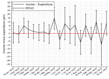
(b) Unadjusted Semi-monthly Panel Dataset: Net income

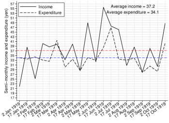
(c) Shifted Semi-monthly Panel Dataset: Income and expenditure

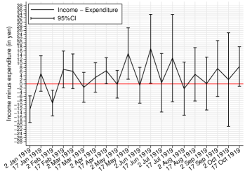
(d) Shifted Semi-monthly Panel Dataset: Net income

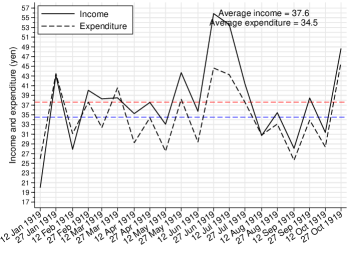
(e) Adjusted Semi-monthly Panel Dataset: Income and expenditure

(f) Adjusted Semi-monthly Panel Dataset: Net income

Figure B.10: Comparisons of Average Monthly Incomes
from Different Aggregations

Note: Figures B.10a, B.10c, B.10e show the average semi-monthly income and expenditure calculated from raw, shifted, and adjusted panel datasets, respectively. Raw series defines the days from the 1st to the 15th of each month as the first half, whereas the days from the 16th to the end of each month as the second half. The shifted series defines the days from the 2nd to the 16th of each month as the first half, whereas the days from the 17th to the 1st of the following month are the second half. Adjusted series is the baseline definition in the main text, which uses the days from 12th to 26th in each month as the “first-half” and those from 27th to 11th in the next month as the “second-half”.

As explained in Section 3, the raw series contains considerable measurement errors due to the timing of payday. The shifted series can deal with the measurement errors from the timing of payday but can not adjust the difference in the payday timing and expenses. In other words, the shifted series ignores the households’ decision on the consumption schedule in each semi-month. The adjusted series can deal with measurement errors and take the timing of the household expenses into account.

Figures B.10b, B.10d, B.10f illustrate the average semi-monthly income minus expenditure calculated from raw, shifted, and adjusted panel datasets, respectively.

Source: Created by the author using the THBS sample.

Figure B.10 explains how different ways of aggregation influence the measured time-series in income and expenditure. Figures B.10a, B.10c, B.10e show the average semi-monthly income and expenditure calculated from raw, shifted, and adjusted panel datasets, respectively.

Raw series defines the days from the 1st to the 15th of each month as the first half and the days from the 16th to the end of each month as the second half. This raw series shall contain substantial measurement errors due to the shifts of paydays explained in Section 3. The time-series plots of average income in Figure B.10a have substantially large variance and fluctuate over time. This is because some semi-monthly income is assigned to the wrong semi-month cells. In these wrong cells, the measured incomes shall take larger values than the actual ones. Moreover, the time-series plots of average expenditure do not chase those of the income. For example, the average expenditure in the second half of June shows a large difference from the average income in the same cell. Consequently, the average net income (i.e., income minus expenditure) in each semi-month is relatively flat and takes a few odd cells with large positive values (Figure B.10b).

The shifted series defines the days from the 2nd to the 16th of each month as the first half and the days from the 17th to the 1st of the following month as the second half. Although the shifted series can deal with the measurement errors from the payday shifts, it can not adjust the difference in the payday timing and expenses. Figure B.10c indeed gets a much smaller variance in the average incomes over time because all the paydays are now fixed to assign the suitable semi-month cells. However, the expenditure series still does not chase the income series well because the payday is placed on the latter edge in each semi-month cell. In other words, the average expenditure in each semi-month reflects a large part of the consumption based on the income of the previous semi-month cell. Since the average incomes take a better series than Figure B.10a, the average net income now seems to show an increasing trend (Figure B.10d). However, it still has a few cells with large negative and large values due to the deviations of expenditure from income.

The adjusted series uses the days from the 12th to 26th of each month as the “first half” and those from the 27th to 11th of the following month as the “second half”. By shifting the entire semi-month cells, this adjusted series can deal with the measurement errors from the payday shifts and fix the miss-matching in the timing of income and expenditure. In other words, each payday is assigned to a suitable semi-month cell, and each semi-month cell reflects the household’s decision on consumption given the latest income. Figure B.10e shows similar time-series plots of average income in Figure B.10c, in which has a corrected semi-monthly average income series. Notably, the expenditure series are now chasing the income series in Figure B.10e because each semi-month cell’s expenditure is based on the income in the same cell. Accordingly, Figure B.10f now shows a smoother series in the net income. It shows a clear increasing trend in the net income and has a smaller variance over time.

These illustrations support the evidence that the adjusted semi-monthly dataset can offer cleaner within variations in income and expenditure because it can fix the measurement errors raised from the shifts of paydays and can reflect the households’ consumption behaviors based on their latest incomes measured in the same semi-month cell.

B.8 Distribution of the Idiosyncratic Shocks

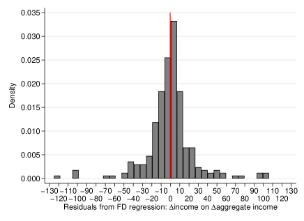
Figure B.11: Distribution of the Idiosyncratic Shocks

Notes: This figure shows the distribution of idiosyncratic shocks in the semi-monthly THBS panel dataset. The idiosyncratic shocks are estimated as the residuals from the regression of the first difference in income on the first difference in aggregate income. The red line indicates the mean of the idiosyncratic shocks ($-0.235$).

Source: Created by the author using the THBS sample.

Figure B.11 illustrates the distribution of the idiosyncratic shocks predicted using the semi-monthly panel dataset. The idiosyncratic shocks are calculated as the residuals from the regression in the first difference in semi-monthly income on the first difference in aggregate semi-monthly income. Let $n_{j}$ be the number of households in semi-month $j$ in the year 1919. For household $i$ in semi-month $j$ cell, the residual is then defined as follows:

$$\Delta\hat{\upsilon}_{i,t}=\Delta\textit{Income}_{i,t}-\hat{\alpha}\Delta\overline{\textit{Income}}_{.,t},$$ (15)

where $\overline{\textit{Income}}_{.,t}=\sum_{i=1}^{n_{t}}\frac{\textit{Income}_{i,t}}{n_{t}}$ and $\hat{\alpha}$ is the estimated coefficient.

It is clear that the residuals satisfy the zero-average property (Figure B.11). However, the residuals have some variations, indicating that the THBS households had experienced both favorable and adverse idiosyncratic shocks during the survey periods.

B.9 Unit Root and Autocorrelations

Table B.5 presents the results of the Fisher-type panel unit root tests for the total expenditure in the semi-monthly (Column 1) and adjusted monthly (Column 2). Both columns show that the null hypothesis of unit roots in all the panels is rejected at the conventional level. The results of the unit root tests for consumption subcategories and variables used to test the risk-coping mechanisms are not reported as those are materially similar results. Since I used the cluster-robust variance-covariance estimator, any arbitrary autocorrelations within unit are allowed in the regressions (Arellano 1987). Despite this, I confirmed that the null hypothesis of no serial correlation is not rejected at the conventional level in Wooldridge’s autocorrelation test for almost of the consumption and net income variables (Wooldridge 2002).

Table B.5: Results of the Unit Root Tests

Test statistics	(1) Semi-Monthly	(2) Adjusted Monthly
$P$-statistic $p$-value	0.0000	0.0001
$Z$-statistic $p$-value	0.0000	0.0000
$L^{*}$-statistic $p$-value	0.0000	0.0000
$P_{m}$-statistic $p$-value	0.0000	0.0000

The results of the Fisher-type panel unit root tests based on augmented Dickey-Fuller (ADF) tests are reported in this table. The null hypothesis is that all the panels contain unit roots, whereas the alternative hypothesis is that at least one panel is stationary. In all the specifications, the process under the null hypothesis is assumed to be a random walk with drift. The demeaned data are used to address the effect of cross-sectional dependence. The number of lagged differences in the ADF regression equation reported is set as one because including two or more two lags reduces a large part of the panel units available for computing the test statistics due to the unbalancedness of the panels. I confirmed that including two lags in the semi-monthly panels does not change the results. Including two lags in the adjusted monthly panels and three lags in the semi-monthly panels is impossible. See Choi (2001) for the details of the tests. These tests need both the first-differenced dependent variable and the lagged dependent variable. Therefore, the units with less than four time-series observations are excluded in the regressions.

Source: Calculated by the author using the THBS sample.

B.10 Risk Preferences

The potential influences of heterogeneous risk preference on standard risk-sharing regressions are discussed in a few works. In my empirical setting, the heterogeneity in the risk preference is assumed to be removed by using the household fixed-effect. When the risk preferences are difference over households, say $\sigma=\sigma_{i}$, equation 26 becomes:

$$\log c_{i,t}=\log c_{t}^{a}+\frac{1}{\sigma_{i}}(\log\omega_{i}-\omega^{a})+(\theta_{i,t}-\theta_{t}^{a}).$$ (16)

The first differencing removes the second term with the coefficient of relative risk aversion in the right-hand side of this equation, even though it varies over the households.

Schulhofer-Wohl (2011) shows that the heterogeneous risk preference may lead to bias in the estimation of the income elasticity under the standard risk-sharing regressions and proposes a parametric test for that heterogeneity. This test is valid under a particular utility function. Specifically, the bias could be raised under the case that the coefficient of relative risk aversion interacts with the aggregate shock in the first-order condition for consumption because the interaction means that the aggregate shock can not be removed using the time-fixed effect in the risk-sharing regressions. As explained, this is a different setting from the one used in the current paper. Mozzoco and Saini (2012) consider a more general case for testing the homogeneity of risk preferences. Their test requires a panel dataset with a very long time dimension that can not be applicable to my THBS dataset.

An alternative way to test potential heterogeneity in the risk preference is to use direct measures on the risk preferences of workers. Schulhofer-Wohl (2011) uses the results of experimental risk-tolerance questions on the workers’ risk preferences in the Health and Retirement Study to test whether the correlations between earnings and aggregate shocks are different across high- and low-risk-tolerance workers. They found that the high-risk-tolerance workers have more procyclical incomes than the low-risk-tolerance workers.

Since the THBS dataset does not have any experimental questions, it is impossible to apply a similar test under my empirical setting. Considering the limitation that the direct test using experimental risk-tolerance question is unavailable, I compare the correlations between the heads’ income and aggregate consumption over sub-groups to get insights into the potential difference in the heads’ attitudes toward risks. For household $i$ and semi-month $t$, the specification is characterized as follows:

$$\log\tilde{y}_{i,t}=\xi_{1}\log c_{t}^{a}+\xi_{2}\log c_{t}^{a}\times d_{i}+ox_{i,t}+\iota_{i}+\varepsilon_{i,t},$$ (19)

where $\tilde{y}_{i,t}$ is head’s earnings, $c_{t}^{a}$ is aggregate consumption, $x_{i,t}$ is the household size, $\iota_{i}$ is the household fixed-effect, and $\varepsilon_{i,t}$ is a random error term. The aggregate consumption is calculated as the cross-sectional average of the total expenditure among THBS sample, given that the mean consumption expenditure among all the skilled factory workers’ households in Tsukishima is unavailable.

$d_{i}$ is an indicator variable that takes one if household $i$ belongs to a specific group that might have had different preferences on their jobs than the other heads in the sample. Firstly, I consider the case that the heads who worked in the large-scale factory had different risk preferences. Although there are no specific anecdotes behind this, the workers in the large-scale factory might have had a lower risk tolerance than those in the small- and medium-scale enterprises. 13 heads who worked in the Ishikawajima shipyard and governmental factory are classified into this group. Secondly, I assume that the heads who worked in the smithing and the non-machinery factories had different risk preferences. As described in Online Appendix A.5, skilled workers in the smithing sector could be business owners. The workers in non-machinery factories might also have different job preferences than the machinery factory workers. This group has only three heads: one worked in a smithing factory, and two worked in food and paper-making factories.

Table B.6 presents the results. In Column (1), the estimated coefficient on the interaction term is close to zero and statistically insignificant. Thus, the sensitivities to aggregate consumption are similar across different scales of the factories. Column (2) further shows that the estimated coefficient on the interaction term is not statistically significant under an alternative proxy of risk tolerance. It suggests that the heads worked in the smithing and non-machinery factories show similar responses to the aggregate shock. Since the aggregate consumption is the cross-sectional sample average, the aggregate variable may contain noise in the period with the small number of cross-sectional observations. To deal with this issue, I exclude the semi-months in October and November 1919 in Columns (3) and (4). Clearly, the estimated coefficients on the interaction terms are largely unchanged in both columns.

This finding is consistent with the fact that these heads have similar characteristics in nature because the budget survey focused on skilled factory workers in Tsukishima. Thus, it would be plausible to see that the THBS households had more or less similar attitudes toward the risks.

Table B.6: Results for Testing Heterogeneous Risk Preferences

	DV: ln(head’s earnings)
	Analytical Period
	(1) Full	(2) Full	Jan. to Sept.	Jan. to Sept.
Aggregate Consumption	0.277*	0.273	0.361**	0.362*
	[0.158]	[0.198]	[0.164]	[0.198]
Aggregate Consumption	-0.041		-0.061
$\times$ Large Scale Factory	[0.453]		[0.415]
Aggregate Consumption		-0.089		-0.178
$\times$ Smithing/Non-machinery		[0.215]		[0.215]
Observations	261	261	239	239

***, **, and * denote statistical significance at the 1%, 5%, and 10% levels, respectively. Standard errors in brackets are clustered at the household level.

Notes: This table shows the results of equation 19 for the semi-monthly panel dataset. ‘Aggregate Consumption’ indicates the cross-sectional sample average of the total expenditures. ‘Large Scale Factory’ indicates an indicator variable that takes one if the head worked in the Ishikawajima shipyard or governmental factory. ‘Smithing/Non-machinery’ indicates an indicator variable that takes one if the head worked in the smithing, food, or paper-making factories. All the regressions include the family size variable and household fixed-effect.

Columns 1–2 show the results for the entire sample period. Columns 2–3 show the results for the period between January and September 1919 to remove year-month cells with the smaller (cross-sectional) number of households (Online Appendix Figure B.4).

Appendix Appendix C Empirical Analysis Appendix

C.1 Conceptual Framework

Consider the economy where household $i=1,...,N$ receives an uncertain income at time $t$ depending on the state of the world $s_{t}\in S_{t}$ as $y_{i,t}(s_{t})$. For infinite time horizon, the state $s_{t}$ realizes with probability $\pi(s_{t})\in[0,1]$. The weighted sum of the expected lifetime utility of $N$ households in the economy is expressed as:

$$\sum_{i=1}^{N}\omega_{i}\sum_{t=0}^{\infty}\rho^{t}\sum_{s_{t}\in S_{t}}\pi(s_{t})u(c_{i,t}(s_{t}),\theta_{i,t}(s_{t})),$$ (20)

where $\omega_{i}$ is the social planner’s weight representing the reciprocal of the marginal utility of each household ($0<\omega_{i}<1$ and $\sum_{i=1}^{N}\omega_{i}=1$), $0<\rho^{t}<1$ is the discount factor, $c_{i,t}(s_{t})$ is households consumption, and $\theta_{i,t}(s_{t})$ is a preference shock. For all states $s_{t}$, the aggregate resource constraint is given by:

$$\sum_{i=1}^{N}c_{i,t}(s_{t})=\sum_{i=1}^{N}e_{i,t}(s_{t}),$$ (21)

where $e_{i,t}(s_{t})$ is household $i$’s exogenous endowment at time $t$.

Following Mace (1991), I assume that the aggregate idiosyncratic shocks approach zero as $N$ gets large. Consider the situation that the household’s endowment can be decomposed into the permanent component ($e_{i,t}^{P}$), shock linked to macroeconomic trends ($\varrho_{i,t}^{a}(s_{t})$), and idiosyncratic shock ($\varsigma_{i,t}(s_{t})$) as:

$$e_{i,t}(s_{t})=e_{i,t}^{P}+\varrho_{i}^{a}(s_{t})+\varsigma_{i,t}(s_{t}).$$ (22)

Given the random nature of the idiosyncratic shock ($\forall t,E[\varsigma_{i,t}(s_{t})|s_{t}]=0$), the sample average of the idiosyncratic shock satisfies $N^{-1}\sum_{i=1}^{N}\varsigma_{i,t}(s_{t})\overset{p}{\to}0$ as $N$ gets large ($\because$ WLLN). This means that the aggregate endowment is written without the idiosyncratic shock as: $e_{t}(s_{t})^{a}=e_{t}^{P,a}+\varrho_{t}^{a}(s_{t})$. Intuitively, the idiosyncratic shocks are shared among the economy with a large number of households.

Subject to equation(21), the social planner maximizes equation(20) by choosing an allocation of consumption across households. The suggested first-order condition at time $t$ is derived as follows:

$$\omega_{i}\rho^{t}\pi(s_{t})u_{c}(c_{i,t}(s_{t}),\theta_{i,t}(s_{t}))=\lambda(s_{t}),$$ (23)

where $\lambda$ is the Lagrange multiplier for the single lifetime resource constraint.

To derive my empirical specification, I assume a constant relative risk aversion preference as:

$$u(c_{i,t}(s_{t}),\theta_{i,t}(s_{t}))=\frac{c_{i,t}^{1-\sigma}(s_{t})}{1-\sigma}\exp(\sigma\theta_{i,t}(s_{t})),$$ (24)

where $\sigma>0$ is the coefficient of relative risk aversion. Below, I consider a particular history of the state of the world so that the subscript $t$ can represent the dependence on the state (e.g., Hayashi et al. 1996). This simplifies the notation in equation 23 as:

$$\omega_{i}\rho^{t}\pi_{t}c_{i,t}^{-\sigma}\text{exp}(\sigma\theta_{i,t})=\lambda_{t}.$$ (25)

Taking the log of equation (25) and aggregating over households, consumption for household $i$ is expressed as:

$$\log c_{i,t}=\log c_{t}^{a}+\frac{1}{\sigma}(\log\omega_{i}-\omega^{a})+(\theta_{i,t}-\theta_{t}^{a}),$$ (26)

where

$$c_{t}^{a}=\exp\left(\frac{1}{N}\sum_{i=1}^{N}\log c_{i,t}\right),~{}~{}~{}~{}~{}\omega^{a}=\frac{1}{N}\sum_{i=1}^{N}\log\omega_{i},~{}~{}~{}~{}~{}\theta_{t}^{a}=\frac{1}{N}\sum_{i=1}^{N}\theta_{i,t}.$$ (27)

The first-difference in equation (26) eliminates the household time-constant effect to yield:

$$\log c_{i,t}-\log c_{i,t-1}=\log c_{t}^{a}-\log c_{t-1}^{a}+(\theta_{i,t}-\theta_{i,t-1})+(\theta_{t}^{a}-\theta_{t-1}^{a}).$$ (28)

Individual income is a conventional proxy variable for the preference shock (Mace 1991). Using the growth rate of household income $\log y_{i,t}-\log y_{i,t-1}$ as a proxy for idiosyncratic shock and adding a measurement error in consumption $\epsilon_{i,t}$, the empirical specification can be characterized as follows:

$$\log c_{i,t}-\log c_{i,t-1}=\alpha_{1}(\log c_{t}^{a}-\log c_{t-1}^{a})+\alpha_{2}(\log y_{i,t}-\log y_{i,t-1})+\epsilon_{i,t}.$$ (29)

The aggregate consumption growth in equation(29) is assumed to reflect macroeconomic shocks in Tsukishima in the case of my empirical setting. As discussed in Section 3.4, the consumption of the THBS households indeed captures the overall macroeconomic trend. Despite this, interpreting $\alpha_{1}$ is not easy because the THBS households include the factory workers’ households in Tsukishima alone. To deal with this potential issue, I use a two-way fixed-effects model instead of the first-difference model in the spirit of Cochrane (1991). Another potential issue is that $\epsilon_{i,t}$ may include the household-specific time-varying preference shock, which might be correlated with the idiosyncratic income shock. Family size influences the household’s preference because the marginal utility of consumption increases with family size (Jappelli and Pistaferri 2017). As explained, the family size had been fairly stable during the sample period in the THBS households, meaning that the preference shifts had rarely occurred (Section 3.4). To be conservative, however, I include the number of family members as a control variable for representing potential preference shock.

Considering these modifications, the empirical specification can finally be characterized as follows:

$$\log c_{i,t}=\gamma\log y_{i,t}+\delta x_{i,t}+\mu_{i}+\phi_{t}+u_{i,t},$$ (30)

where $c_{i,t}$ is consumption, $y_{i,t}$ is disposable income, $x_{i,t}$ is family size, $\mu_{i}$ is the household fixed effect, $\phi_{t}$ is the time fixed effect, and $u_{i,t}$ is a random error term. The estimate of $\gamma$ shall range from zero (i.e., idiosyncratic shocks are perfectly insured) to one (for the absence of insurance).

In order to test the risk-coping mechanisms, I consider the following representation of individual consumption in the spirit of Fufchamps and Lund (2003).

$$c_{i,t}=y_{i}^{P}+y_{i,t}^{T}+r_{i,t},$$ (31)

where $y_{i}^{P}$ is permanent income and $y_{i,t}^{T}$ is transitory income. $r_{i,t}=\bm{z}^{\prime}_{i,t}\bm{1}$ is a linear combination of the net temporary incomes expressed using a $k\times 1$ net income vector ($\bm{z}$) and a vector of ones. Substituting equation 31 into equation 26 and taking the first-difference removes the time-constant components, including the permanent income. It follows that my empirical specification can be characterized as follows:

$$r_{i,t}=\kappa\tilde{y}_{i,t}+\eta x_{i,t}+\nu_{i}+\zeta_{t}+\epsilon_{i,t},$$ (32)

where $\tilde{y}_{i,t}$ is head’s earning, $x_{i,t}$ is the family size control, $\nu_{i}$ indicates the household-fixed effect, $\zeta_{t}$ indicates the time-fixed effect, and $\epsilon_{i,t}$ is a random error term. I herein use the head’s earnings ($\tilde{y}_{i,t}$) as the idiosyncratic shock variable instead of the disposable income. The regression is separately run for each component in the net income vector ($\bm{z}$).

C.2 Raw Relationship between Income and Expenditures

Figure C.1 summarizes the densities of the log-differences (LD) of the semi-monthly expenditures. Figure C.1a illustrates the LD distribution of the total expenditure, whereas Figures C.1b–C.1l summarize the LD distributions of the 11 subcategories of the expenditure. These figures confirm no specific outliers in all these expenditure categories.

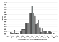
(a) Total expenditure

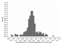
(b) Food

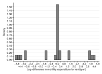
(c) Housing

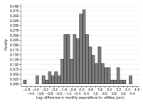
(d) Utilities

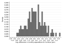
(e) Furniture

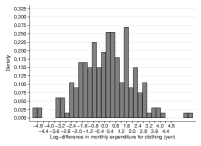
(f) Clothing

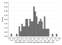
(g) Education

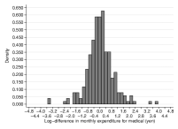
(h) Medical

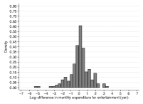
(i) Entertainment

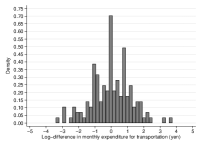
(j) Transportation

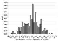
(k) Gift

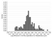
(l) Miscellaneous

Figure C.1: Distributions of the Log-differences of the Semi-monthly Expenditures

Notes: The distribution of the log-difference in semi-monthly total expenditure is shown in Figure C.1a. Figures C.1b–C.1l show the distributions of the log-differences in semi-monthly expenditure for the 11 subcategories listed in panel A of Table 3.

Sources: Created by the author using the THBS sample.

Figure C.4 summarizes the scatter plots between the LD of the semi-monthly disposable income and expenditures. Figure C.2a illustrates the relationship between the LD of the semi-monthly disposable income and total expenditure. Figures C.2b–C.2l illustrate the correlations between the LD of the semi-monthly disposable income and 11 expenditure subcategories.

Generally, rent was paid once per month. This means that the semi-monthly dataset fails to capture the variations in rent payment because it includes some semi-monthly cells with zero values. In addition, the water bills are included in the rent subcategory but not in the utility subcategory. This means that a semi-month cell takes a minimal value when the payment of rent is not included in that cell. Figure C.1c indeed shows that the LD of rent generates some larger values in the semi-monthly panel dataset due to those water bill payments. These cells taking large LD values substantially increased the slope, as shown in Figure C.2c.

Given this technical issue, I used the adjusted monthly panel dataset to analyze the estimate for the rent category. I confirmed that the adjusted monthly panel dataset (Online Appendix B.7) can assign the rent payday each month. The scatter plot from the adjusted monthly variation shows a flat relationship in Figure C.4c.

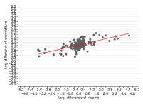
(a) Total expenditure

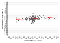
(b) Food

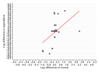
(c) Housing

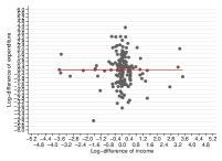
(d) Utilities

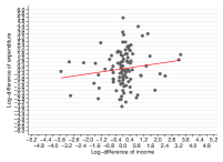
(e) Furniture

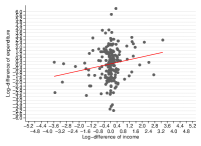
(f) Clothing

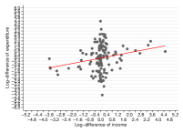
(g) Education

(h) Medical

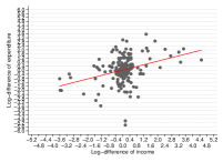
(i) Entertainment

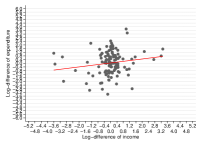
(j) Transportation

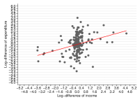
(k) Gift

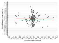
(l) Miscellaneous

Figure C.2: Raw Relationship between the Log-differences in Semi-monthly Income and Expenditure

Notes: Figure C.2a illustrates the relationship between the log-differences in semi-monthly income and expenditure. Figures C.2b–C.2l illustrate the relationships between the log-differences in semi-monthly disposable income and the 11 expenditure subcategories listed in Panel A in Table 3. The range of the y-axis is fixed across all the figures for comparability.

Sources: Created by the author using the THBS sample.

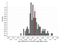
(a) Total expenditure

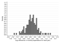
(b) Food

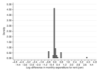
(c) Housing

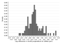
(d) Utilities

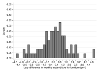
(e) Furniture

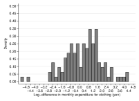
(f) Clothing

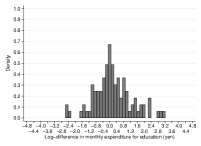
(g) Education

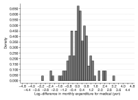
(h) Medical

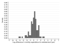
(i) Entertainment

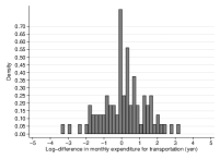
(j) Transportation

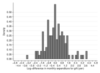
(k) Gift

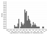
(l) Miscellaneous

Figure C.3: Distributions of the Log-differences of the Monthly Expenditures

Notes: The distribution of the log-difference in adjusted monthly total expenditure is shown in Figure C.3a. Figures C.3b–C.3l show the distributions of the log-differences in adjusted monthly expenditure for the 11 subcategories listed in panel A of Table 3.

Sources: Created by the author using the THBS sample.

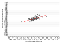
(a) Total expenditure

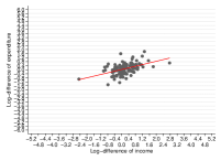
(b) Food

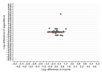
(c) Housing

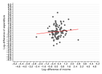
(d) Utilities

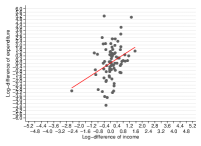
(e) Furniture

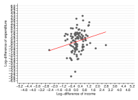
(f) Clothing

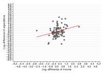
(g) Education

(h) Medical

(i) Entertainment

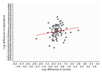
(j) Transportation

(k) Gift

(l) Miscellaneous

Figure C.4: Raw Relationship between the Log-differences in Monthly Income and Expenditure

Notes: Figure C.4a illustrates the relationship between the log-differences in semi-monthly income and expenditure. Figures C.4b–C.4l illustrate the relationships between the log-differences in semi-monthly disposable income and the 11 expenditure subcategories listed in Panel A in Table 3. The range of the y-axis is fixed across all the figures for comparability.

Sources: Created by the author using the THBS sample.

C.3 Retail Sales in Tokyo City: A Retail Store Survey of 1935

Table C.1 summarizes the contribution of regular customers to their total sales, social classes of the customers, and sales methods in the retailers selling white rice, fish, greengrocers, and fuels (firewood and charcoal) by the scale of their businesses. In the original document, the figures for the sales method (Columns 8–10) in firewood and charcoal shops (Total) are missing. For these three cells, I filled the averages over the three business-size categories in each sales method: 20.4% for “Cash”, 78.4% for “Credit purchase”, and 1.3% for “Monthly installment”.

Table C.1: Customers, Sales Methods, and Competitiveness in the Retailers in Tokyo City

Selling Item	Scale of	Number of	Share of sales	Social Class of			Sales Method (%)			Number of
	Business	stores	for regular	the Regular Customer (%)			Cash	Credit	Monthly	competitors
		reported	customer (%)	Upper	Middle	Other		purchase	installment	reported
White Rice	Small	19	69.7	12.1	49.5	38.4	29.5	70.2	0.3	7.3
	Medium	55	69.5	17.5	41.6	40.9	26.9	72.6	0.5	8.7
	Large	27	81.7	15.9	51.5	32.6	26.7	71.0	2.3	8.8
	Total	101	73.1	16	45.7	38.2	26.9	71.5	1.7	8.5
Fish	Small	34	64.5	5.9	53.2	40.9	42.7	57.3	0	5.1
	Medium	20	62.6	10	58.0	32.0	43.8	56.2	0	5.3
	Large	5	72.0	0	86.0	14.0	44.8	55.2	0	3.4
	Total	59	64.6	6.8	57.6	35.6	43.9	56.1	0	5.0
Greengrocer	Small	46	42.2	8	39.2	52.7	59.7	40.3	0	6.5
	Medium	17	57.1	8.8	43.5	47.6	65.0	35.0	0	6.1
	Large	3	36.7	33.3	40.0	26.7	79.7	20.3	0	3.7
	Total	66	45.4	9.4	40.4	50.2	65.8	34.2	0	6.2
Firewood and charcoal	Small	78	68.5	13.5	50.7	35.8	25.0	74.2	0.8	8.4
	Medium	17	77.7	23.5	49.1	27.4	19.3	79.1	1.6	8.9
	Large	5	33.3	23.0	60.0	17.0	16.8	81.8	1.4	10.6
	Total	100	51.1	15.7	50.9	33.4	20.4	78.4	1.3	8.6

Notes:

This table summarizes the statistics on the sales in the retail shops selling white rice, fish, fruit and vegetables, and firewood and charcoal in Tokyo surveyed in 1935.

1. Small, middle, and large-scale businesses include retailers with annual sales of less than 10,000, 10,000–30,000, and 30,000+ yen, respectively.

2. The number of stores reported the share of regular customers (column 4) are 90, 56, 61, and 93 in the white rice, fish, greengrocers, and firewood and charcoal categories, respectively.

3. The share of regular customers is defined as the percentage of sales for regular customers in the annual total sales in 1935.

4. The definition of the social classes (“Upper”; “Middle”; “Other”) is not clearly defined in the report. Therefore, this must be based on the subjective judgment of the retailers.

5. The share of sales method is based on the percentage of sales using each method in the annual total sales in 1935.

6. The number of competitors indicates the number of peers within a three-cho (approximately 327 meters) radius.

Source: Tokyo City Chamber of Commerce and Industry 1937, pp. legend; 20–21; questionnaire.

References

- Aguila et al. (2017) Emma Aguila, Arie Kapteyn, and Francisco Perez-Arce. Consumption smoothing and frequency of benefit payments of cash transfer programs. The American Economic Review, 107(5):430–435, May 2017.
- Arellano (1987) Manuel Arellano. Computing robust standard errors within groups estimator. Oxford Bulletin of Economics and Statistics, 49:431–434, 1987.
- Arrow and Debreu (1954) Kenneth J Arrow and Gerard Debreu. Existence of an equilibrium for a competitive economy. Econometrica, 22(3):265–290, July 1954.
- Asdrubali et al. (2020) Pierfederico Asdrubali, Simone Tedeschi, and Luigi Ventura. Household risk-sharing channels. Quantitative Economics, 11(3):1109–1142, July 2020.
- Attanasio and Pistaferri (2016) Orazio P Attanasio and Luigi Pistaferri. Consumption inequality. Journal of Economic Perspectives, 30(2):3–28, May 2016.
- Baltagi et al. (2012) Badi H Baltagi, Chihwa Kao, and Long Liu. On the estimation and testing of fixed effects panel data models with weak instruments. In Terrell Daniel and Millimet Dek, editors, Advances in Econometrics (30th Anniversary Edition), volume 30, pages 199–235. Emerald Group Publishing Limited, United Kingdom, 2012.
- Blundell et al. (2016) Richard Blundell, Luigi Pistaferri, and Itay Saporta-Eksten. Consumption inequality and family labor supply. The American Economic Review., 106(2):387–435, 2016.
- Boyer (1997) George R Boyer. Poor relief, informal assistance, and short time during the lancashire cotton famine. Explorations in Economic History, 34(1):56–76, January 1997.
- Cai et al. (2012) Zongwu Cai, Ying Fang, and Henong Li. Weak instrumental variables models for longitudinal data. Econometric Reviews, 31(4):361–389, July 2012.
- Cochrane (1991) John H Cochrane. A simple test of consumption insurance. Journal of Political Economy, 99(5):957–976, 1991.
- Comola and Prina (2023) Margherita Comola and Silvia Prina. The interplay among savings accounts and network-based financial arrangements: Evidence from a field experiment. The Economic Journal, 133(649):516–535, 2023.
- Dercon (2004) Stefan Dercon. Insurance Against Poverty. Oxford University Press, 11 2004.
- Dynarski et al. (1997) Susan Dynarski, Jonathan Gruber, Robert A Moffitt, and Gary Burtless. Can families smooth variable earnings? Brookings Papers on Economic Activity, 1997(1):229–303, 1997.
- Fafchamps and Lund (2003) Marcel Fafchamps and Susan Lund. Risk-sharing networks in rural philippines. Journal of Development Economics, 71(2):261–287, August 2003.
- Foster (1995) Andrew D Foster. Prices, credit markets and child growth in Low-Income rural areas. The Economic Journal, 105(430):551–570, 1995.
- Francks (2009) Penelope Francks. The Japanese Consumer: An Alternative Economic History of Modern Japan. University of Cambridge Press, Cambridge, 2009.
- Gertler and Gruber (2002) Paul Gertler and Jonathan Gruber. Insuring consumption against illness. The American Economic Review, 92(1):51–70, 2002.
- Gervais and Klein (2010) Martin Gervais and Paul Klein. Measuring consumption smoothing in CEX data. Journal of Monetary Economics, 57(8):988–999, November 2010.
- Gordon (2013) Andrew Gordon. Fabricating Consumers: The Sewing Machine in Modern Japan. University of California Press, Calfornia, 2013.
- Grimard (1997) Franque Grimard. Household consumption smoothing through ethnic ties: evidence from cote d’ivoire. Journal of Development Economics, 53(2):391–422, August 1997.
- Gruber (1997) Jonathan Gruber. The consumption smoothing benefits of unemployment insurance. The American Economic Review, 87(1):192–205, 1997.
- Henderson and Turner (2020) J Vernon Henderson and Matthew A Turner. Urbanization in the developing world: Too early or too slow? Journal of Economic Perspectives, 34(3):150–173, August 2020.
- Horn et al. (1975) Susan D Horn, Roger A Horn, and David B Duncan. Estimating Heteroscedastic Variances in Linear Models. Journal of the American Statistical Association, 70(350):380–385, June 1975.
- Horrell and Oxley (2000) Sara Horrell and Deborah Oxley. Work and prudence: Household responses to income variation in nineteenth-century britain. European Review of Economic History, 4(1):27–57, April 2000.
- James and Suto (2011) John A James and Isao Suto. Early twentieth-century japanese worker saving: precautionary behaviour before a social safety net. Cliometrica, 5(1):1–25, January 2011.
- Jappelli and Pistaferri (2017) Tullio Jappelli and Luigi Pistaferri. The Economics of Consumption: Theory and Evidence. Oxford University Press, New York, October 2017.
- Kantor and Fishback (1996) Shawn Everett Kantor and Price V Fishback. Precautionary saving, insurance, and the origins of workers’ compensation. Journal of Political Economy, 104(2):419–442, 1996.
- Kiesling (1996) L Lynne Kiesling. Institutional choice matters: The poor law and implicit labor contracts in victorian lancashire. Explorations in Economic History, 33(1):65–85, 1996.
- Kuznets (1962) Simon Kuznets. Quantitative aspects of the economic growth of nations: VII. the share and structures of consumption. Economic Development and Cultural Change, 10(2):1–92, 1962.
- Mace (1991) Barbara J Mace. Full insurance in the presence of aggregate uncertainty. Journal of Political Economy, 99(5):928–956, 1991.
- Macours et al. (2022) Karen Macours, Patrick Premand, and Renos Vakis. Transfers, diversification and household risk strategies: Can productive safety nets help households manage climatic variability? The Economic Journal, 132(647):2438–2470, March 2022.
- Mazzocco and Saini (2012) Maurizio Mazzocco and Shiv Saini. Testing efficient risk sharing with heterogeneous risk preferences. The American Economic Review, 102(1):428–468, 2012.
- Meyer and Sullivan (2023) Bruce D Meyer and James X Sullivan. Consumption and income inequality in the united states since the 1960s. Journal of Political Economy, 131(2):247–284, 2023.
- Miyamoto (2008) Matao Miyamoto. Economic History of Japan [in Japanese]. Hōsōdaigaku Kyōikushinkōkai, Tokyo, 2008.
- Morduch (1999) Jonathan Morduch. Theory and evidence from indian households. March 1999.
- Nakamura (1971) Takafusa Nakamura. Analysis of Economic Growth in prewar Japan [in Japanese]. Iwanami Shoten, Tokyo, 1971.
- Nakamura and Odaka (1989) Takafusa Nakamura and Konosuke Odaka. Overview. In Takafusa Nakamura and Konosuke Odaka, editors, Dual-Structure [in Japanese], pages 1–80. Iwanami Shoten, Tokyo, 1989.
- Nelson (1994) Julie A Nelson. On testing for full insurance using consumer expenditure survey data. Journal of Political Economy, 102(2):384–394, 1994.
- O’Connell and Reid (2005) Sean O’Connell and Chris Reid. Working-Class consumer credit in the UK, 1925-60: The role of the check trader. The Economic History Review, 58(2):378–405, 2005.
- Ogasawara (2024) Kota Ogasawara. Consumption smoothing in the working-class households of interwar japan. The Journal of Economic History, 84(1):111–147, 2024.
- Pearson (1900) Karl Pearson. On the criterion that a given system of deviations from the probable in the case of a correlated system of variables is such that it can be reasonably supposed to have arisen from random sampling. Philosophical Magazine, 50(302):157–175, July 1900.
- Ravallion and Chaudhuri (1997) Martin Ravallion and Shubham Chaudhuri. Risk and insurance in village india: Comment. Econometrica, 65(1):171–184, 1997.
- Rose (1999) Elaina Rose. Consumption smoothing and excess female mortality in rural india. The Review of Economics and Statistics, 81(1):41–49, February 1999.
- Rosenzweig and Stark (1989) Mark R Rosenzweig and Oded Stark. Consumption smoothing, migration, and marriage: Evidence from rural india. Journal of Political Economy, 97(4):905–926, August 1989.
- Sawai and Tanimoto (2016) Minoru Sawai and Masayuki Tanimoto. The Economic History of Japan: From the Early Modern Era to the Present [in Japanese]. Yūhikaku, Tokyo, 2016.
- Schneider and Ogasawara (2018) Eric B Schneider and Kota Ogasawara. Disease and child growth in industrialising japan: Critical windows and the growth pattern, 1917-39. Explorations in Economic History, 69:64–80, 2018.
- Schulhofer-Wohl (2011) Sam Schulhofer-Wohl. Heterogeneity and tests of risk sharing. Journal of Political Economy, 119(5):925–958, 2011.
- Scott and Walker (2012) Peter M Scott and James Walker. Working-Class household consumption smoothing in interwar britain. The Journal of Economic History, 72(3):797–825, August 2012.
- Sekiya (1970) Koichi Sekiya. Seikatsu koten sōsho, volume 6: Tsukishima chōsa (A classic series of books about life, volume 6: Tsukishima Survey) [in Japanese]. Kōseikan, Tokyo, 1970.
- Shibuya and Shojiro (1982) Kameji Suzuki. Shibuya, Ryuichi. and Ishiyama Shojiro. Nihon no shichiya (Pawn Shops in Japan) [in Japanese]. Waseda University Press, Tokyo, 1982.
- Skoufias and Quisumbing (2005) Emmanuel Skoufias and Agnes R Quisumbing. Consumption insurance and vulnerability to poverty: A synthesis of the evidence from bangladesh, ethiopia, mali, mexico and russia. The European Journal of Development Research, 17(1):24–58, March 2005.
- Staiger and Stock (1997) B Y Douglas Staiger and James H Stock. Instrumental variables regression with weak instruments. Econometrica, 65(3):557–586, 1997.
- Tanimoto (2002) Masayuki Tanimoto. Small business in the modern japanese city. In Takafusa Nakamura and Fujii Nobuyuki, editors, Urbanization and Conventional Industry [in Japanese], pages 1–50. Chuō Keizai Sha, Tokyo, 2002.
- Tanimoto (2011) Masayuki Tanimoto. Kindainihon no setaikeizai to jyoseirōdō (women’s work and household economy in modern japan) [in japanese]. Ohara Shakaimondai Kenkyūjyo zasshi, 635_636:7–25, September 2011.
- Tanimoto (2012) Masayuki Tanimoto. The role of housework in everyday life: Another aspect of consumption in modern japan. In Penelope Francks and Hunter Janet, editors, The Historical Consumer, pages 27–55. Palgrave Macmillan, New York, 2012.
- Townsend (1994) Robert M Townsend. Risk and insurance in village india. Econometrica, 62(3):539–591, 1994.
- Townsend (1995) Robert M Townsend. Consumption insurance: An evaluation of Risk-Bearing systems in Low-Income economies. Journal of Economic Perspectives, 9(3):83–102, 1995.
- Udry (1994) Christopher Udry. Risk and insurance in a rural credit market: An empirical investigation in northern nigeria. The Review of Economic Studies, 61(3):495–526, July 1994.
- Udry (1995) Christopher Udry. Risk and saving in northern nigeria. The American Economic Review, 85(5):1287–1300, 1995.
- Uyeki et al. (2022) Timothy M Uyeki, David S Hui, Maria Zambon, David E Wentworth, and Arnold S Monto. Influenza. Lancet, 400(10353):693–706, August 2022.
Documents and Database
- (1)
- (2) Central Federation of Industrial Associations. Sangyō kumiai chōsa siryō, volume 9 (Survey report of the industrial association, volume.9). [in Japanese] Tokyo: Central Federation of Industrial Associations, 1925.
- (3)
- (4) Ohkawa, Kazushi, Miyohei Shinohara, and Mataji Umemura. Estimates of Long-term Economic Statistics of Japan since 1868, volume.8. [in Japanese] Tokyo: Toyo Keizai Shinposha, 1967.
- (5)
- (6) Ohkawa, Kazushi, Takamatsu Nobukiyo, and Yamamoto Yuzo. Estimates of Long-term Economic Statistics of Japan since 1868, volume.1. [in Japanese] Tokyo: Toyo Keizai Shinposha, 1974.
- (7)
- (8) Statistics Bureau of the Cabinet. Nihonteikoku shiintōkei (The statistics of causes of death of the empire Japan, 1918 edition). [in Japanese]. Statistics Bureau of the Cabinet, Tokyo, 1921.
- (9)
- (10) Statistics Bureau of the Cabinet. Nihonteikoku shiintōkei (The statistics of causes of death of the empire Japan, 1919 edition). [in Japanese]. Statistics Bureau of the Cabinet, Tokyo, 1922.
- (11)
- (12) Statistics Bureau of the Cabinet. Nihonteikoku shiintōkei (The statistics of causes of death of the empire Japan, 1920 edition). [in Japanese]. Statistics Bureau of the Cabinet, Tokyo, 1923.
- (13)
- (14) Statistics Bureau of the Cabinet. Taishō kyūnen kokusei chōsa hōkoku, zenkoku no bu, dai ikkan (Population Census of Japan, Vol. 1, 1920 Edition). [in Japanese] Tokyo: Statistics Bureau of the Cabinet, 1928.
- (15)
- (16) Statistics Bureau of the Cabinet. Taoshō kyūnen kokuseichōsahōkoku, zenkoku no bu, dai nikan (Population Census of Japan, Vol. 2, 1920 Edition). [in Japanese] Tokyo: Statistics Bureau of the Cabinet, 1929a.
- (17)
- (18) Statistics Bureau of the Cabinet. Taishō kyūnen kokusei chōsa hōkoku, zenkoku no bu, dai sankan (Population Census of Japan, Vol. 3, 1920 Edition). [in Japanese] Tokyo: Statistics Bureau of the Cabinet, 1929b.
- (19)
- (20) Statistics Bureau of the Cabinet. Taishō kyūnen kokusei chōsa hōkoku, fuken no bu, dai ikkan (Population Census of Japan, Tokyo Prefecture, 1920 Edition). [in Japanese] Tokyo: Statistics Bureau of the Cabinet, 1929c.
- (21)
- (22) Tokyo City Office. Tokyoshi tōkeisho, dai jyūnana kai (Annual Statistics of the City of Tokyo, volume 17) [in Japanese]. Tokyo: Tokyo City Office, 1921.
- (23)
- (24) Tokyo City Office. Tokyo shi shisei tōkei genpyō, dai ikkan (Tokyo City Municipal Statistics Original Table, vol.1) [in Japanese]. Tokyo: Tokyo City Office, 1922a.
- (25)
- (26) Tokyo City Office. Tokyo shi shisei tōkei genpyō, dai nikan (Tokyo City Municipal Statistics Original Table, vol.2) [in Japanese]. Tokyo: Tokyo City Office, 1922b.
- (27)
- (28) Tokyo City Office. Tokyo shi shisei tōkei genpyō, dai sankan (Tokyo City Municipal Statistics Original Table, vol.3) [in Japanese]. Tokyo: Tokyo City Office, 1922c.
- (29)
- (30) Tokyo City Statistics Division. Tokyo shi oyobi kinkō chōson rōdōtōkeigenpyō (dai ikkai, dai nikan) (Labor Statistics Table for Tokyo City and Suburbs, issue 2 of volume 1) [in Japanese]. Tokyo: Tokyo City Office, 1926a.
- (31)
- (32) Tokyo City Social Affairs Bureau.Tokyo shinai saimin no nyūshichi nikansuru chōsa (Survey on the use of pawnshops among the poor in Tokyo City) [in Japanese]. Tokyo City Social Affairs Bureau, 1921.
- (33)
- (34) Tokyo Institute for Municipal Research. Toshishominkinyū nikansuru chōsa, dainisatsu toshichochiku ginkō (Survey of Financial Institution among Common People, volume. 2, Municipal Savings Banks) [in Japanese]. Tokyo Institute for Municipal Research, 1925b.
- (35)
- (36) Tokyo Institute for Municipal Research. Toshishominkinyū nikansuru chōsa, daiyonsatsu kousetsu shichiho (Survey of Financial Institutions among Common People, volume. 2, Pubic pawnshops) [in Japanese]. Tokyo Institute for Municipal Research, 1926.
- (37)
- (38) Department of Health, Ministry of the Interior. Tokyo-shi Kyobashi-ku Tsukishima ni okeru jicchichōsahōkoku (dai isshū) (Report of the Field Study in Tsukishima in Kyobashi Ward of Tokyo City, Volume 1) [in Japanese]. Tokyo: Department of Health, Ministry of the Interior, 1923a.
- (39)
- (40) Department of Health, Ministry of the Interior. Tokyo-shi Kyobashi-ku Tsukishima ni okeru jicchichōsahōkoku (dai isshū, furoku no ichi) (Report of the Field Study in Tsukishima in Kyobashi Ward of Tokyo City, Appendix 1 of Volume 1) [in Japanese]. Tokyo: Department of Health, Ministry of the Interior, 1923b.
- (41)
- (42) Department of Health, Ministry of the Interior. Tokyo-shi Kyobashi-ku Tsukishima ni okeru jicchichōsahōkoku (dai isshū, furoku no ni) (Report of the Field Study in Tsukishima in Kyobashi Ward of Tokyo City, Appendix 2 of Volume 1) [in Japanese]. Tokyo: Department of Health, Ministry of the Interior, 1923c.
- (43)
- (44) Ministry of Agriculture and Commerce. Kōjyō Tsūran (Taishō jyūnen jyūgatsu) (Handbook of Factories, November 1921 edition) [in Japanese]. Tokyo: Ministry of Agriculture and Commerce, 1921.
- (45)
- (46) Ministry of Land, Infrastructure, Transport and Tourism (database). Gyōsei kuiki data (Administrative area data) [in Japanese]. (https://nlftp.mlit.go.jp/ksj/gml/datalist/KsjTmplt-N03-v2˙2.html, accessed on 15th August 2023).
- (47)
- (48) National Police Agency.Keisatsuchō tōkeisho (Statistics of National Police Agency, 1918 edition). [in Japanese] Tokyo: Documentation Division, Superintendent General’s Office, 1920a.
- (49)
- (50) National Police Agency.Keisatsuchō tōkeisho (Statistics of National Police Agency, 1919 edition). [in Japanese] Tokyo: Documentation Division, Superintendent General’s Office, 1920b.
- (51)
Archival Sources
- (1)
- (2) The Ohara Institute for Social Research, Archives of the Tsukishima Survey (THBS, unreleased).
- (3) The Ohara Institute for Social Research, Archives of Gonda Yasunosuke (7-2).
- (4) The Ohara Institute for Social Research, Archives of Gonda Yasunosuke (7-3).
- (5) The Ohara Institute for Social Research, Archives of Gonda Yasunosuke (7-4).
- (6)