On optimal tracking portfolio in incomplete markets: The classical control and the reinforcement learning approaches

Abstract

This paper studies an infinite horizon optimal tracking portfolio problem using capital injection in incomplete market models. We consider the benchmark process modelled by a geometric Brownian motion with zero drift driven by some unhedgeable risk. The relaxed tracking formulation is adopted where the portfolio value compensated by the injected capital needs to outperform the benchmark process at any time, and the goal is to minimize the cost of the discounted total capital injection. In the first part, we solve the stochastic control problem when the market model is known, for which the equivalent auxiliary control problem with reflections and the associated HJB equation with a Neumann boundary condition are studied. In the second part, the market model is assumed to be unknown, for which we consider the exploratory formulation of the control problem with entropy regularizer and develop the continuous-time q-learning algorithm for the stochastic control problem with state reflections. In an illustrative example, we show the satisfactory performance of the q-learning algorithm.

Keywords: Optimal tracking portfolio, capital injection, incomplete market, stochastic control with reflection, continuous-time reinforcement learning, q-learning

1 Introduction

One important business in fund management is to choose the portfolio among some risky assets to closely track some benchmark processes such as the market index, the inflation rates, the exchange rates, the liability, or the living cost and education cost, etc. How to formulate the tracking procedure and derive the optimal tracking portfolio has become an active research topic in quantitative finance during the past decades. For example, several objectives for active portfolio management are proposed in Browne (1999a), Browne (1999b), and Browne (2000) including: maximizing the probability that the agent’s wealth achieves a performance goal related to the benchmark before falling below a predetermined shortfall; minimizing the expected time to reach the performance goal; the mixture of these two objectives, and some further extensions by considering the expected reward or expected penalty. Another standard method to optimize the tracking error is to minimize the variance or downside variance relatively to the index value or return, which leads to the linear-quadratic stochastic control problem; See Gaivoronski et al. (2005), Yao et al. (2006) and Ni et al. (2022) among others. In Strub and Baumann (2018), a different objective function is introduced to measure the similarity between the normalized historical trajectories of the tracking portfolio and the index where the rebalancing transaction costs can also be taken into account. Recently, another new tracking formulation using the fictitious capital injection is studied in Bo et al. (2021, 2023a, 2023b), however, all in the complete market model. With the help of an auxiliary control problem based on the constructing state process with reflections, the original stochastic control problem under dynamic floor constraints is then equivalent to the study of the HJB equation with a Neumann boundary condition. The market completeness plays a key role therein as the dual transform of the HJB equation leads to a linear PDE problem whose solution admits some probabilistic representations. The existence of the classical solution for the linear PDE and the verification of the feedback optimal portfolio control can be obtained by using stochstic flow analysis and some delicate estimations.

The present paper aims to further extend the studies on the relaxed tracking portfolio using capital injection in Bo et al. (2021, 2023a, 2023b) in some incomplete market models in which there exists some unhedgeable risk driving the external benchmark process (see (2.4)). As a direct consequence, the previous methodology based on the dual transform and the probabilistic representations for the dual PDE therein fails because the dual HJB equation can no longer be linearized. We therefore only consider the benchmark process governed by a geometric Brownian motion with zero drift in the present paper. We propose two different approaches in two cases when the precise information of the market model is given and when the market model is unknown, respectively.

In the first problem in which the information of the market model is given, we adopt the equivalent formulation to the auxiliary control problem similar to Bo et al. (2021), which is to solve a stochastic control problem when the auxiliary state process exhibits reflections at the boundary $0$. By taking advantage of the benchmark dynamics as a geometric Brownian motion, the dimension reduction of the control problem can be exercised. For the obtained one-dimensional control problem, the classical solution to the associated HJB equation with a Neumann boundary condition can be solved fully explicitly. As a result, the optimal portfolio control can be characterized in an explicit feedback form and the verification on its optimality can be established.

In the second part of the paper, we consider the more realistic situation when the market model is unknown, for which we are interested in developing the continuous-time reinforcement learning approach. Recently, for continuous-time stochastic control problems, Wang et al. (2020), Jia and Zhou (2022a, b, 2023) have developed the theoretical foundation for reinforcement learning in the continuous time exploration formulation with continuous state space and action space. In particular, Wang et al. (2020) firstly studied the exploratory learning formulation by incorporating the entropy regularization to encourage the policy exploration, and the optimal policy has been shown therein as a Gaussian type for LQ control problems. Jia and Zhou (2022a) examined the policy evaluation problem and proposed the martingale loss to facilitate the algorithm design. The policy gradient problem was then studied in Jia and Zhou (2022b) where the martingale approach in Jia and Zhou (2022a) can be adopted for the policy gradient and some Actor-Critic algorithms can be devised to learn the value function and the stochastic policies alternatively. Later, Jia and Zhou (2023) established a continuous time q-learning theory by considering the first order approximation of the conventional discrete-time Q-function. We also refer to some recent subsequent studies in different contexts such as Wang et al. (2023) in developing the continuous-time Actor-Critic algorithm for solving the optimal execution problem in the Almgren-Chriss model; the application of policy improvement algorithm in Bai et al. (2023) for solving the optimal dividend problem in diffusion models; and the generalization of continuous-time q-learning in Wei and Yu (2023) for mean-field control problems in McKean-Vlasov diffusion models.

In this paper, we are interested in generalizing the continuous-time q-learning from the standard controlled diffusion models in Jia and Zhou (2023) to solve our auxiliary stochastic control problem with the reflection boundary at $0$. In particular, for the stochastic control problems with reflections, it is shown in the present paper that the value function and the associated q-function can also be characterized by the martingale condition of some stochastic processes involving the reflection term or the local time at $0$; see Proposition 4.2 and Theorem 4.3. In addition, some extra transversality conditions (see (4.16) and (4.17)) are also needed in our infinite horizon setting. Building upon our martingale characterization in Theorem 4.3, we are able to devise the offline q-learning algorithm for the targeted stochastic control problems with reflections using the loss function resulting from the martingale orthogonality condition. As a new theoretical contribution to the literature, in the context of the infinite horizon stochastic control problems with reflections, we establish the convergence of the stochastic approximation algorithms for time discretization and horizon truncation when $\Delta t\rightarrow 0$ and $T\rightarrow\infty$; see Theorem 4.5. To illustrate the efficiency of our q-learning algorithm, we study a simulation example of our optimal tracking portfolio problem with a particular choice of the temperature parameter $\gamma=\rho/d$. Here $\rho$ stands for the subjective discount rate and $d$ is the dimension of stocks, both are known to the agent. In this case, we present an example beyond the LQ control framework such that the exploratory HJB equation with a Neumann boundary condition can be solved fully explicitly, allowing us to obtain the exact parameterization of the optimal value function and the optimal q-function. For some initial inputs and choices of learning rates, we illustrate the very satisfactory performance of the iteration convergence of learned parameters towards their true values.

The remainder of this paper is organized as follows. Section 2 introduces the incomplete market model and the benchmark process as well as the portfolio optimization problem under the relaxed tracking formulation using capital injection. Section 3 studies the classical control problem when the market model is known, where the auxiliary control problem formulation and the dimension reduction are employed such that the HJB equation can be solved explicitly and the optimal feedback control can be derived and verified. In Section 4, the market model is assumed to be unknown, the continuous-time reinforcement learning approach is proposed for the exploratory formulation of the control problem with entropy regularizer. In particular, the q-learning algorithm is developed therein together with some convergence results on time discretization and horizon truncation. Section 5 presents a simulation example with a specific temperature parameter beyond the LQ control framework such that the value function and q-function still admit exact parameterizations. Finally, all proofs of the main results in previous sections are reported in Section 6.

2 Market Model and Problem Formulation

In this section, we introduce the market model and formulate our optimal tracking problem. Let $(\Omega,\mathcal{F},\mathbb{F}^{W},\mathbb{P}^{W})$ be a filtered probability space with the filtration $\mathbb{F}^{W}=(\mathcal{F}^{W}_{t})_{t\geq 0}$ satisfying the usual conditions. This filtered probability space supports a $d+1$-dimensional Brownian motion $(W^{0},W^{1},\ldots,W^{d})=(W_{t}^{0},W_{t}^{1},\ldots,W_{t}^{d})_{t\geq 0}$. Consider a financial market consisting of $d$ risky assets driven by the $d$-dimensional Brownian motion $W=(W^{1},\ldots,W^{d})^{\top}$. In other words, the price process $S^{i}=(S_{t}^{i})_{t\geq 0}$ of the $i$-th asset is described as the following Black-Scholes model, for $t\geq 0$,

$$\frac{dS_{t}^{i}}{S_{t}^{i}}=\mu_{i}dt+\sum_{j=1}^{d}\sigma_{ij}dW_{t}^{j},\quad i=1,\ldots,d,$$ (2.1)

where, for $i,j=1,\ldots,d$, the coefficient $\mu_{i}\in\mathds{R}$ is the return rate and the coefficient $\sigma_{ij}\in\mathds{R}$ denotes the volatility. Hereafter, denote by $\mu=(\mu_{1},\ldots,\mu_{d})^{\top}$ the vector of return rate and by $\sigma=(\sigma_{ij})_{d\times d}$ the volatility matrix. Assume that the riskless interest rate $r=0$ that amounts to the change of numéraire and the return rate $\mu\neq{\bm{0}}$. From this point onwards, all processes including the wealth process and the benchmark process are defined after the change of numéraire.

For $t\geq 0$, let $\theta_{t}^{i}$ be the amount of wealth (the resulting process $\theta^{i}=(\theta_{t}^{i})_{t\geq 0}$ is assumed to be $\mathbb{F}^{W}$-adapted) that the fund manager allocates in asset $S^{i}=(S_{t}^{i})_{t\geq 0}$ at time $t$. The self-financing wealth process under the portfolio control $\theta=(\theta_{t}^{1},\ldots,\theta_{t}^{d})_{t\geq 0}^{\top}$ is given by, for $t\geq 0$,

$$V^{\theta}_{t} =\textrm{v}+\int_{0}^{t}\theta_{s}^{\top}\mu ds+\int_{0}^{t}\theta_{s}^{\top}\sigma dW_{s},\quad V_{0}^{\theta}=\textrm{v}\in\mathds{R}_{+}:=[0,\infty).$$ (2.2)

We consider the portfolio decision making by the fund manager whose goal is to optimally track a stochastic benchmark process $Z=(Z_{t})_{t\geq 0}$. In the present paper, we consider the benchmark process satisfying the geometric Brownian motion (GBM) in the form of

$$\frac{dZ_{t}}{Z_{t}}=\sigma_{Z}dW^{\kappa}_{t},\quad\forall t>0$$ (2.3)

with the initial value $Z_{0}=z>0$ and the volatility $\sigma_{Z}>0$. For the nonzero correlative coefficient $\kappa\in[-1,1]$, the process $W^{\kappa}=(W_{t}^{\kappa})_{t\geq 0}$ appeared in (2.3) is a standard Brownian motion, which is defined by

$$W^{\kappa}_{t}:=\kappa W^{0}_{t}+\sqrt{1-\kappa^{2}}W^{\eta}_{t},\quad t\geq 0.$$ (2.4)

Here $W^{\eta}=(W^{\eta}_{t})_{t\geq 0}$ is a linear combination of the $d$-dimensional Brownian motion $W$ with weights $\eta=(\eta_{1},\ldots,\eta_{d})^{\top}\in[-1,1]^{d}$, which itself is a Brownian motion. We also recall that $W^{0}=(W^{0}_{t})_{t\geq 0}$ is a Brownian motion independent of the $d$-dimensional Brownian motion $W$. The type of benchmark process $Z$ in (2.3) may refer to futures price process for a commodity, a stock index, or an interest rate index, see, for example, the benchmark considered in Björk and Landén (2000).

Given the benchmark process $Z=(Z_{t})_{t\geq 0}$, an optimal tracking portfolio problem is considered that combines the portfolio control with another singular control as capital injection together with dynamic floor constraints. To be precise, we assume that the fund manager can strategically inject capital $A=(A_{t})_{t\geq 0}$ into the fund account from time to time whenever it is necessary such that the total capital dynamically dominates the benchmark process $Z$, i.e., $A_{t}+V_{t}^{\theta}\geq Z_{t}$ for all $t\geq 0$. The goal of the optimal tracking problem is to minimize the expected cost of the discounted total capital injection under dynamic floor constraints that

$${\rm w}(\mathrm{v},z):=\text{$\inf_{A,\theta}\mathbb{E}\left[A_{0}+\int_{0}^{\infty}e^{-\rho t}dA_{t}\right]$\quad s.t.\quad$Z_{t}\leq A_{t}+V^{\theta}_{t}$ at each $t\geq 0$,}$$ (2.5)

where the constant $\rho>0$ is the discount rate and $A_{0}=(z-\textrm{v})^{+}$ is the initial injected capital to match with the initial benchmark.

To cope with the problem (2.5) with dynamic floor constraints, we observe that, for a fixed control $\theta$, the optimal $A$ is the smallest adapted right-continuous and non-decreasing process that dominates $Z-V^{\theta}$. Let $\mathbb{U}$ be the set of regular $\mathbb{F}$-adapted control processes $\theta=(\theta_{t})_{t\geq 0}$ such that (2.2) is well-defined. Similar to Bo et al. (2021), for each fixed regular control $\theta$, the optimal singular control $A_{t}^{*}$ satisfies that

$$A^{*}_{t}=0\vee\sup_{s\in[0,t]}(Z_{s}-V_{s}^{\theta}),\quad\forall t\geq 0.$$ (2.6)

As a result, the problem (2.5) with floor constraints admits the equivalent formulation as a unconstrained control problem but with a running maximum cost that

$${\rm w}(\mathrm{v},z)=(z-\mathrm{v})^{+}+\inf_{\theta\in\mathbb{U}}\ \mathbb{E}\left[\int_{0}^{\infty}e^{-\rho t}d\left(0\vee\sup_{s\in[0,t]}(Z_{s}-V_{s}^{\theta})\right)\right].$$ (2.7)

In the forthcoming section, we will focus on the solvability of problem (2.7) in the sense of strong control by introducing an auxiliary control problem.

3 The Classical Strong Control Approach

In this section, we will first introduce an auxiliary stochastic control problem closely related to the unconstrained stochastic control problem (2.7), and then apply the dimension reduction and solve the associated one-dimensional HJB equation with a Neumann boundary condition.

3.1 Auxiliary control problem

To formulate the auxiliary control problem, we impose a new controlled state process to replace the process $V^{\theta}=(V_{t}^{\theta})_{t\geq 0}$ given in (2.2). To do it, we first define the following difference process by

$$D_{t}:=Z_{t}-V_{t}^{\theta}+\mathrm{v}-z,\quad\forall t\geq 0.$$ (3.1)

It is obvious that $D_{0}=0$. Moreover, for any $x\geq 0$, let us consider the running maximum process of $D=(D_{t})_{t\geq 0}$ defined by

$$L_{t}:=x\vee\sup_{s\in[0,t]}D_{s}\geq 0,\quad\forall t>0,$$ (3.2)

with the initial value $L_{0}=x\geq 0$. One can easily see that $(z-\mathrm{v})^{+}-{\rm w}(z,\mathrm{v})$ with the value function ${\rm w}(\mathrm{v},z)$ given in (2.7) is equivalent to the auxiliary control problem:

$$\sup_{\theta\in\mathbb{U}}\mathbb{E}\left[-\int_{0}^{\infty}e^{-\rho t}dL_{t}\right],$$ (3.3)

when we set the initial level $L_{0}=x=(\mathrm{v}-z)^{+}$.

We start with the introduction of a new controlled state process $X=(X_{t})_{t\geq 0}$ for problem (3.3), which is defined as the reflected process $X_{t}:=L_{t}-D_{t}$ for $t\geq 0$ that satisfies the SDE:

$$X_{t}=-\int_{0}^{t}\sigma_{Z}Z_{s}dW^{\kappa}_{s}+\int_{0}^{t}\theta_{s}^{\top}\mu ds+\int_{0}^{t}\theta_{s}^{\top}\sigma dW_{s}+L_{t},\quad\forall t\geq 0$$ (3.4)

with the initial value $X_{0}=x\geq 0$. In particular, the running maximum process $L_{t}$ increases if and only if $X_{t}=0$, i.e., $L_{t}=D_{t}$. We will change the notation from $L_{t}$ to $L_{t}^{X}$ from this point onwards to emphasize its dependence on the new state process $X$ given in (3.4). The benchmark process $Z=(Z_{t})_{t\geq 0}$ defined in (2.3) is chosen as another state process.

Let $\mathbb{U}^{r}$ be the set of admissible portfolios (controls) such that the reflected SDE (3.4) has a unique strong solution. Then, we propose the following stochastic control problem, for $(x,z)\in\mathds{R}_{+}\times(0,\infty)$,

$$\hat{{\rm w}}(x,z):=\sup_{\theta\in\mathbb{U}^{r}}J(\theta;x,z):=\sup_{\theta\in\mathbb{U}^{r}}\mathbb{E}_{x,z}\left[-\int_{0}^{\infty}e^{-\rho t}dL_{t}^{X}\right],$$ (3.5)

where $\mathbb{E}_{x,z}[\cdot]:=\mathbb{E}[\cdot|X_{0}=x,Z_{0}=z]$. Using the definition (3.5) of $\hat{\rm w}(x,z)$, it is not difficult to check that (i) the value function $x\to\hat{{\rm w}}(x,z)$ is non-decreasing; (ii) it holds that $\sup_{x_{1},x_{2}\geq 0}|\frac{\hat{{\rm w}}(x_{1},z)-\hat{{\rm w}}(x_{2},z)}{x_{1}-x_{2}}|\leq 1$, that is, the value function $x\to\hat{{\rm w}}(x,z)$ is Lipschitz continuous with Lipschitz coefficient being $1$. These properties will be applied in the remaining sections.

3.2 Reduction of dimension

In this section, we apply the change of measure to simplify the stochastic control problem in (3.5) by reducing the dimension. To this end, let us introduce the normalized processes of triplet $(X,\theta,L^{X})$ by the benchmark process $Z=(Z_{t})_{t\geq 0}$ defined by

$$Y_{t}:=\frac{X_{t}}{Z_{t}},\quad\tilde{\theta}_{t}:=\frac{\theta_{t}}{Z_{t}},\quad L_{t}^{Y}:=\int_{0}^{t}\frac{dL_{s}^{X}}{Z_{s}},\quad\forall t\geq 0.$$ (3.6)

Note that the process $Z$ is strictly positive (see (2.3)). Then, $t\to L_{t}^{Y}$ is a non-decreasing process and satisfies that, a.s.

$$\int_{0}^{t}{\bf 1}_{Y_{s}=0}dL_{s}^{Y}=\int_{0}^{t}{\bf 1}_{X_{s}=0}\frac{dL_{s}^{X}}{Z_{s}}=\int_{0}^{t}\frac{dL_{s}^{X}}{Z_{s}}=L_{t}^{Y},\quad\forall t\geq 0.$$

This implies that $L^{Y}=(L_{t}^{Y})_{t\geq 0}$ is the local time process for the process $Y=(Y_{t})_{t\geq 0}$ at the reflecting boundary $0$. Then, the Itô’s rule yields that

$$dY_{t} =\sigma_{Z}^{2}(Y_{t}+1)dt-\sigma_{Z}(Y_{t}+1)dW_{t}^{\kappa}+\tilde{\theta}_{t}^{\top}\mu dt+\tilde{\theta}_{t}^{\top}\sigma dW_{t}+dL_{t}^{Y}.$$ (3.7)

In the sequel, we introduce the following change of measure specified by

$$\frac{d\mathbb{Q}^{W}}{d\mathbb{P}^{W}}\Big{|}_{\mathcal{F}_{t}}=Z_{t},\quad\forall t\geq 0.$$ (3.8)

We then consider the following stochastic control problem formulated as:

$$u(y) :=\sup_{\theta\in\tilde{\mathbb{U}}^{r}}\mathbb{E}^{\mathbb{Q}^{W}}\left[-\int_{0}^{\infty}e^{-\rho s}dL_{s}^{Y}\right],\quad\forall y\in\mathds{R}_{+},$$ (3.9)

where the normalized admissible set $\tilde{\mathbb{U}}^{r}:=\{(\frac{\theta_{t}}{Z_{t}})_{t\geq 0};\leavevmode\nobreak\ \theta\in\mathbb{U}^{r}\}$, and $\mathbb{E}^{\mathbb{Q}}[\cdot]$ is the expectation under the probability measure $\mathbb{Q}^{W}\sim\mathbb{P}^{W}$. It follows from (3.7) that the underlying state process $Y$ has the following dynamics under $\mathbb{Q}^{W}$ given by

$$dY_{t} =-\sigma_{Z}(Y_{t}+1)d\tilde{W}^{\kappa}_{t}+\tilde{\theta}^{\top}_{t}\mu dt+\tilde{\theta}^{\top}_{t}\sigma dW_{t}+dL_{t}^{Y}.$$ (3.10)

Here $\tilde{W}_{t}^{\kappa}:=W^{\kappa}_{t}-\sigma_{Z}t$ for $t\geq 0$ is a $\mathbb{Q}^{W}$-Brownian motion. For the case $\kappa=1$, the process $\tilde{W}^{\kappa}=(\tilde{W}_{t}^{\kappa})_{t\geq 0}$ is also independent of $W=(W^{1},\ldots,W^{d})^{\top}$. The following lemma gives the relationship between the value function $u(y)$ for $y\geq 0$ defined by (3.9) and the value function $\hat{\rm w}(x,z)$ for $(x,z)\in\mathds{R}_{+}\times(0,\infty)$ defined by (3.5).

Lemma 3.1.

Let $(x,z)\in\mathds{R}_{+}\times(0,\infty)$. It holds that $\hat{\rm w}(x,z)=zu\left(\frac{x}{z}\right)$.

The proof of Lemma 3.1 is reported in Section 6.

3.3 HJB equation and verification result

Lemma 3.1 tells us that we can solve the simplified stochastic control problem (3.9) with one-dimensional state process instead of problem (3.5). Then, the corresponding value function satisfies the following HJB equation given by, for $y>0$,

$$\sup_{\tilde{\theta}\in\mathds{R}^{n}}\left\{u^{\prime}(y)\tilde{\theta}^{\top}\mu+u^{\prime\prime}(y)\tilde{\theta}^{\top}\sigma\sigma^{\top}\tilde{\theta}-\sqrt{1-\kappa^{2}}\sigma_{Z}(y+1)\tilde{\theta}^{\top}\sigma\eta u^{\prime\prime}(y)\right\}$$

$$\qquad+\frac{1}{2}\sigma_{Z}^{2}(y+1)^{2}u^{\prime\prime}(y)=\rho u(y)$$ (3.11)

with Neumann boundary condition $u^{\prime}(0)=1$. If the value function $u$ is strictly concave, then the optimal feedback portfolio is given by

$$\tilde{\theta}^{*}(y)=-(\sigma\sigma^{\top})^{-1}\frac{u^{\prime}(y)\mu-\sqrt{1-\kappa^{2}}\sigma_{Z}(y+1)\sigma\eta u^{\prime\prime}(y)}{u^{\prime\prime}(y)},\quad\forall y\geq 0.$$ (3.12)

By plugging (3.12) into (3.3), we have

$$-\alpha\frac{(u^{\prime}(y))^{2}}{u^{\prime\prime}(y)}+\sqrt{1-\kappa^{2}}\zeta(y+1)u^{\prime}(y)+\frac{1}{2}\sigma_{Z}^{2}\kappa^{2}(y+1)^{2}u^{\prime\prime}(y)=\rho u(y),$$ (3.13)

where the coefficients are defined by $\alpha:=\frac{1}{2}\mu^{\top}(\sigma\sigma^{\top})^{-1}\mu$ and $\zeta:=\sigma_{Z}\eta^{\top}\sigma^{-1}\mu$. We consider the candidate solution of Eq. (3.13) given by

$$u(y)=\frac{\lambda-1}{\lambda}(1+y)^{\frac{\lambda}{\lambda-1}},\quad y\geq 0.$$ (3.14)

Here, $\lambda\in(0,1)$ is the unique solution to the following equation:

$$\ell(\lambda):=\alpha\lambda(\lambda-1)^{2}+\rho(\lambda-1)^{2}-\sqrt{1-\kappa^{2}}\zeta\lambda(\lambda-1)-\frac{1}{2}\kappa^{2}\sigma_{Z}^{2}\lambda=0.$$ (3.15)

In fact, one can easily check that

$$\lim_{\lambda\to-\infty}\ell(\lambda)=-\infty,\quad\ell(0)=\rho>0,\quad\ell(1)=-\frac{1}{2}\kappa^{2}\sigma_{Z}^{2}<0,\quad\lim_{\lambda\to+\infty}\ell(\lambda)=+\infty.$$

Therefore, Eq. (3.15) has a unique root $\lambda\in(0,1)$.

Based on the above results, we have the following verification result for the classical strong control problem.

Theorem 3.2.

The function $u(y)$ for $y\geq 0$ given by (3.14) is a classical solution of the HJB equation (3.3). Define the following optimal feedback control function by, for all $y\in\mathds{R}_{+}$,

$$\tilde{\theta}^{*}(y)=(1-\lambda)(y+1)(\sigma\sigma^{\top})^{-1}\mu+\sqrt{1-\kappa^{2}}\sigma_{Z}(y+1)(\sigma\sigma^{\top})^{-1}\sigma\eta.$$ (3.16)

Consider the controlled state process $Y^{*}=(Y_{t}^{*})_{t\geq 0}$ that obeys the following SDE, for all $t\geq 0$,

$$Y_{t}^{*}=-\int_{0}^{t}\sigma_{Z}(Y_{s}+1)d\tilde{W}^{\kappa}_{s}+\int_{0}^{t}\tilde{\theta}^{*}(Y_{s}^{*})^{\top}\mu ds+\int_{0}^{t}\tilde{\theta}^{*}(Y_{s}^{*})^{\top}\sigma dW_{s}+L_{t}^{Y^{*}},$$ (3.17)

with $L_{0}^{Y^{*}}=y$. Let $\tilde{\theta}_{t}^{*}=\tilde{\theta}^{*}(Y_{t}^{*})$ for all $t\geq 0$, then $\tilde{\theta}^{*}=(\tilde{\theta}_{t}^{*})_{t\geq 0}\in\tilde{\mathbb{U}}^{\mathrm{r}}$ is an optimal investment strategy. That is, for all admissible $\tilde{\theta}\in\tilde{\mathbb{U}}^{\mathrm{r}}$, we have

$$\mathbb{E}^{\mathbb{Q}^{W}}\left[-\int_{0}^{\infty}e^{-\rho t}dL_{t}^{Y}\right]\leq u(y),\quad\forall y\in\mathds{R}_{+},$$

where the equality holds when $\tilde{\theta}=\tilde{\theta}^{*}$.

The proof of Theorem 3.2 is provided in Section 6.

Remark 3.3.

Note that the optimal feedback control $\tilde{\theta}^{*}(y)$ is linear in $(y+1)$, thereby the optimal control $\theta^{*}_{t}$ admits the feedback form of $\theta^{*}_{t}=\theta^{*}(X^{*}_{t},Z^{*}_{t})$ where the feedback function $\theta^{*}(x,z)$ is linear in $(x+z)$ in view of the relationship documented in (3.6). Then, recall the definition of $X_{t}$ in (3.4), when the wealth process $V_{t}^{\theta^{*}}\geq Z_{t}$, the optimal portfolio $\theta^{*}_{t}$ is also linear in $V_{t}^{\theta^{*}}$, i.e., it is optimal to invest a fraction of the wealth into stocks whenever the wealth process itself can already outperform the benchmark process.

4 The Continuous-time Reinforcement Learning Approach

In this section, the model is assumed to be unknown to the fund manager, i.e., all model parameters $\mu=(\mu_{1},\ldots,\mu_{d})^{\top}$, $\sigma=(\sigma_{ij})_{d\times d}$, $\sigma_{Z}$, $\kappa$ and $\eta=(\eta_{1},\ldots,\eta_{d})^{\top}\in[-1,1]^{d}$ are unknown. Thereby, the classical control approach in the previous section is not applicable. Our goal is to develop a continuous-time reinforcement learning algorithm to find the optimal tracking portfolio in problem (3.9).

Reinforcement learning allows the decision maker to learn the optimal action in the unknown environment through the interactions with the environment as the repeated trial-and-error procedure. Specifically, the agent exercises a sequel of actions $\tilde{\theta}=(\tilde{\theta}_{t})_{t\geq 0}$ and observe responses from $(Y^{\tilde{\theta}},L^{Y})=(Y^{\tilde{\theta}}_{t},L_{t}^{Y})_{t\geq 0}$ along with a stream of discounted running rewards $(-e^{-\rho t}dL_{t}^{Y})_{t\geq 0}$, and continuously update and improve his actions based on these observations.

To describe the exploration step in reinforcement learning, we can randomize the pair of action $\tilde{\theta}$ and consider the joint distribution. Assume that the probability space is rich enough to support uniformly distributed random variables on $[0,1]$ that is independent of $(\tilde{W}^{\kappa},W^{1},\ldots,W^{d})$, and then such a uniform random variable can be used to generate other random variables with specified density functions. Let $K=(K_{t})_{t\in[0,T]}$ be a process of mutually independent copies of a uniform random variable on $[0,1]$ which is also independent of the BMs $(W^{0},W^{1},\ldots,W^{d})$, the construction of which requires a suitable extension of probability space (c.f. Sun 2006). We then further expand the filtered probability space to $(\Omega,\mathcal{F},\mathbb{F},\mathbb{Q})$ where $\mathbb{F}=(\mathcal{F}_{t}^{W}\vee\sigma\left(K_{s},0\leq s\leq t\right))_{t\geq 0}$ and the probability measure $\mathbb{Q}$, now defined on $\mathbb{F}$, is an extension from $\mathbb{Q}^{W}$ (i.e. the two probability measures coincide when restricted to $\mathbb{F}^{W}$). In particular, let $\bm{\pi}:y\in\mathds{R}_{+}\to\bm{\pi}(\cdot\mid y)\in\mathcal{P}({\cal A})$ be a given (feedback) policy whith ${\cal A}:=\mathds{R}^{d}$, and $\mathcal{P}({\cal A})$ is a suitable collection of probability density functions. At each time $t\geq 0$, an action $\tilde{\theta}^{\bm{\pi}}_{t}$ is generated from the joint density $\bm{\pi}\left(\cdot\mid Y_{t}\right)$. Fix a policy $\bm{\pi}$ and an initial state $y\geq 0$, we can consider the following reflected SDE:

$$dY_{t}^{\bm{\pi}} =-\sigma_{Z}(Y_{t}^{\bm{\pi}}+1)d\tilde{W}^{\kappa}_{t}+(\tilde{\theta}^{\bm{\pi}}_{t})^{\top}\mu dt+(\tilde{\theta}^{\bm{\pi}}_{t})^{\top}\sigma dW_{t}+dL_{t}^{Y^{\bm{\pi}}},\leavevmode\nobreak\ t>0;\quad Y^{\bm{\pi}}_{0}=y.$$ (4.1)

Here, $L^{Y^{\bm{\pi}}}=(L_{t}^{Y^{\bm{\pi}}})_{t\geq 0}$ denotes the local time of the state process $Y^{\bm{\pi}}=(Y_{t}^{\bm{\pi}})_{t\geq 0}$ at the level $0$.

To encourage exploration, we adopt the Shannon’s entropy regularizer suggested in Wang et al. (2020) that leads to the following value function associated to a given policy $\bm{\pi}$ that

$$J(y;\bm{\pi})=\mathbb{E}^{\mathbb{Q}}\left[-\gamma\int_{0}^{\infty}e^{-\rho t}\ln{\bm{\pi}}\left(\tilde{\theta}_{t}^{{\bm{\pi}}}\mid Y^{\bm{\pi}}_{t}\right)\mathrm{d}t-\int_{0}^{\infty}e^{-\rho t}dL_{t}^{Y^{\bm{\pi}}}\Big{|}Y_{0}^{\bm{\pi}}=y\right],$$ (4.2)

where $\mathbb{E}^{\mathbb{Q}}$ is the expectation with respect to both the Brownian motion and the action randomization. In the above, $\gamma>0$ is a given parameter indicating the level of exploration, also known as the temperature parameter.

Similar to Wang et al. (2020), we can show that the average of the sample trajectories $(Y^{\bm{\pi}}_{t})_{t\geq 0}$ converges to $(\tilde{Y}_{t}^{\bm{\pi}})_{t\geq 0}$, which satisfies the following reflected SDE:

$$d\tilde{Y}_{t}^{\bm{\pi}}=\tilde{b}(\tilde{Y}^{\bm{\pi}}_{t},\bm{\pi}(\cdot\mid\tilde{Y}^{\bm{\pi}}_{t}))dt+\tilde{\sigma}(\tilde{Y}^{\bm{\pi}}_{t},\bm{\pi}(\cdot\mid\tilde{Y}^{\bm{\pi}}_{t}))dB_{t}+dL_{t}^{\bm{\pi}},$$ (4.3)

where $B=(B_{t})_{t\geq 0}$ is a standard Brownian independent of $(\tilde{W}^{\kappa},W)$, and the coefficient functions $(\tilde{b},\tilde{\sigma})$ are respectively defined by, for $(y,\bm{\pi})\in\mathds{R}_{+}\times\mathcal{P}(\mathcal{A})$,

$$\begin{cases}\displaystyle\tilde{b}(y,\bm{\pi}):=\int_{\mathcal{A}}\tilde{\theta}^{\top}\mu\bm{\pi}(\tilde{\theta}\mid y)d\tilde{\theta},\\[11.99998pt] \displaystyle\tilde{\sigma}(y,\bm{\pi}):=\sqrt{\int_{\mathcal{A}}\left(\frac{1}{2}\tilde{\theta}^{\top}\sigma\sigma^{\top}\tilde{\theta}-\sqrt{1-\kappa^{2}}\sigma_{Z}(y+1)\tilde{\theta}^{\top}\sigma\eta+\frac{\sigma_{Z}^{2}}{2}(y+1)^{2}\right)\bm{\pi}(\tilde{\theta}\mid y)d\tilde{\theta}}.\end{cases}$$

It follows from the property of Markovian projection in Brunick and Shreve (2013) that $Y_{t}^{\bm{\pi}}$ and $\tilde{Y}_{t}^{\bm{\pi}}$ have the same distribution for any $t\geq 0$. As a consequence, the value function (4.2) is equivalent to the following relaxed control form (see also Kushner (1990) and Fleming (1999)):

$$J(y;\bm{\pi})=\mathbb{E}^{\mathbb{Q}^{W}}\left[-\gamma\int_{0}^{\infty}e^{-\rho t}\int_{\mathcal{A}}\ln\bm{\pi}\left(\tilde{\theta}\mid\tilde{Y}_{t}^{\bm{\pi}}\right)\bm{\pi}\left(\tilde{\theta}\mid\tilde{Y}_{t}^{\bm{\pi}}\right)d\tilde{\theta}dt-\int_{0}^{\infty}e^{-\rho t}dL_{t}^{\bm{\pi}}\Big{|}\tilde{Y}_{0}^{\bm{\pi}}=y\right].$$ (4.4)

The task of reinforcement learning is to find the optimal policy to attain the maximum of the value function that

$$v(y)=\max_{\bm{\pi}\in\Pi}J(y;\bm{\pi}),\quad y\geq 0,$$ (4.5)

where the set $\Pi$ stands for the set of admissible (stochastic) policies. The following gives the precise definition of admissible policies.

Definition 4.1.

A policy $\bm{\pi}$ is called admissible, that is, $\pi\in\Pi$, if

• $\bm{\pi}$ takes the feedback form as $\bm{\pi}_{t}={\bm{\pi}}(\cdot|Y_{t})$ for $t\geq 0$, where $\bm{\pi}(\cdot|\cdot):{\cal A}\times\mathds{R}_{+}\to\mathds{R}$ is a measurable function and $\bm{\pi}(\cdot|y)\in{\cal P}({\cal A})$ for all $y\in\mathds{R}_{+}$;

• the SDE (4.3) admits a unique strong solution for any initial $y\in\mathds{R}_{+}$.

Assume that the value function (4.4) under a given admissible policy $\bm{\pi}\in\Pi$ is smooth enough, we can see that it satisfies the following Neumann problem, for $\bm{\pi}\in\mathcal{P}(\mathcal{A})$,

$$\begin{cases}\displaystyle\int_{\mathcal{A}}\left[H(\tilde{\theta},y,J_{y}(y;\bm{\pi}),J_{yy}(y;\bm{\pi}))-\gamma\ln\bm{\pi}(\tilde{\theta}\mid y)\right]\bm{\pi}(\tilde{\theta}\mid y)d\tilde{\theta}\\[8.00003pt] \displaystyle\qquad\qquad\qquad\qquad\qquad\qquad\qquad+\frac{\sigma_{Z}^{2}}{2}(y+1)^{2}J_{yy}(y;\bm{\pi})=\rho J(y;\bm{\pi}),\\[10.00002pt] \displaystyle J_{y}(0;{\bm{\pi}})=1.\end{cases}$$ (4.6)

On the other hand, the optimal value function defined by (4.5) satisfies the following exploratory HJB equation with a Neumann boundary condition that, for $y\geq 0$,

$$\begin{cases}\displaystyle\sup_{{\bm{\pi}}\in{\mathcal{P}}({\mathcal{A}})}\int_{\mathcal{A}}\left[H(\tilde{\theta},y,v_{y}(y),v_{yy}(y))-\gamma\ln\bm{\pi}(\tilde{\theta})\right]\bm{\pi}(\tilde{\theta})d\tilde{\theta}+\frac{\sigma_{Z}^{2}}{2}(y+1)^{2}v_{yy}(y)=\rho v(y),\\[16.99998pt] \displaystyle v_{y}(0)=1.\end{cases}$$ (4.7)

Here, the Hamilton operator $H:{\cal A}\times\mathds{R}_{+}\times\mathds{R}\times\mathds{R}\to\mathds{R}$ is defined by

$$H(\tilde{\theta},y,P,Q):=\tilde{\theta}^{\top}\mu P+\frac{1}{2}\tilde{\theta}^{\top}\sigma\sigma^{\top}\tilde{\theta}Q-\sqrt{1-\kappa^{2}}\sigma_{Z}(y+1)\tilde{\theta}^{\top}\sigma\eta Q.$$ (4.8)

Moreover, by assuming $v_{yy}<0$, the candidate optimal policy is a Gaussian measure after normalization that

$${\bm{\pi}}^{*}(\tilde{\theta}\mid y) =\frac{\exp\left\{\frac{1}{\gamma}H(\tilde{\theta},y,v_{y}(y),v_{yy}(y))\right\}}{\int_{\mathcal{A}}\exp\left\{\frac{1}{\gamma}H(\tilde{\theta},y,v_{y}(y),v_{yy}(y))\right\}d\tilde{\theta}}$$

$$=\mathcal{N}\left(\tilde{\theta}\leavevmode\nobreak\ \Big{|}-(\sigma\sigma^{\top})^{-1}\frac{\mu v_{y}(y)-\sqrt{1-\kappa^{2}}\sigma_{Z}(y+1)\sigma\eta v_{yy}(y)}{v_{yy}(y)},-(\sigma\sigma^{\top})^{-1}\frac{\gamma}{v_{yy}(y)}\right),$$ (4.9)

where we have denoted by ${\cal N}(\tilde{\theta}|a,b)$ the Gaussian density function with mean vector $a\in\mathds{R}^{d}$ and covariance matrix $b\in\mathds{R}^{d\times d}$.

In what follows, we use the Gaussian policy in (4) to establish the policy improvement theorem.

Theorem 4.1 (Policy Improvement Theorem).

For any given $\bm{\pi}\in\Pi$, assume that the value function $J(\cdot;\bm{\pi})\in C^{2}(\mathds{R}_{+})$ satisfies Eq. (4.6) with the Neumann boundary condition and $J_{yy}(\cdot;{\bm{\pi}})<0$ for any $y\in\mathds{R}_{+}$. We consider the mapping ${\cal I}$ on $\Pi$ defined by

$$\mathcal{I}(\bm{\pi}) :=\frac{\exp\left\{\frac{1}{\gamma}H(\cdot,y,J_{y}(y;\bm{\pi}),J_{yy}(y;\bm{\pi}))\right\}}{\int_{\mathcal{A}}\exp\left\{\frac{1}{\gamma}H(\tilde{\theta},y,J_{y}(y;\pi),J_{yy}(y;\bm{\pi}))\right\}d\tilde{\theta}}$$

$$=\mathcal{N}\left(\tilde{\theta}\leavevmode\nobreak\ \Big{|}-(\sigma\sigma^{\top})^{-1}\frac{\mu J_{y}(y;\bm{\pi})-\sqrt{1-\kappa^{2}}\sigma_{Z}(y+1)\sigma\eta J_{yy}(y;\bm{\pi})}{J_{yy}(y;\bm{\pi})},-(\sigma\sigma^{\top})^{-1}\frac{\gamma}{J_{yy}(y;\bm{\pi})}\right).$$

Then, we have

• Denote by ${\bm{\pi}}^{\prime}={\cal I}(\bm{\pi})$. If ${\bm{\pi}}^{\prime}\in\Pi$ satisfies

  $$\lim_{T\to\infty}\mathbb{E}^{\mathbb{Q}^{W}}\left[e^{-\rho T}J(\tilde{Y}_{T}^{{\bm{\pi}}^{\prime}};\bm{\pi})\right]=0,$$ (4.10)

  then it holds that

  $$J\left(y;\bm{\pi}^{\prime}\right)\geq J(y;\bm{\pi}),\quad\forall y\in\mathds{R}_{+}.$$

• If the map ${\cal I}$ has a fixed point $\bm{\pi}^{*}\in\Pi$ satisfying

  $$\begin{cases}\displaystyle\lim_{T\to\infty}\mathbb{E}^{\mathbb{Q}^{W}}\left[e^{-\rho T}J(\tilde{Y}_{T}^{{\bm{\pi}}^{*}};\bm{\pi}^{*})\right]=0,\\[11.99998pt] \displaystyle\limsup_{T\to\infty}\mathbb{E}^{\mathbb{Q}^{W}}\left[e^{-\rho T}J(\tilde{Y}_{T}^{{\bm{\pi}}};\bm{\pi}^{*})\right]\geq 0,\quad\forall{\bm{\pi}}\in\Pi,\end{cases}$$ (4.11)

  then $\bm{\pi}^{*}$ is the optimal policy that

  $$v(y)=\max_{\bm{\pi}\in\Pi}J(y;\bm{\pi})=J(y;\bm{\pi}^{*}).$$

• In particular, if we choose the the temperature parameter $\gamma=\frac{\rho}{d}$, the map ${\cal I}$ has an explicit fixed point $\bm{\pi}^{*}\in\Pi$ given by

  $$\bm{\pi}^{*}(\cdot|y)=\mathcal{N}\left(y\leavevmode\nobreak\ \Big{|}(\sigma\sigma^{\top})^{-1}(\mu+\sigma_{z}\sqrt{1-\kappa^{2}}\sigma\eta)(1+y),(\sigma\sigma^{\top})^{-1}\gamma(1+y)^{2}\right).$$ (4.12)

Theorem 4.1-(i) provides a theoretical result for the policy improvement iteration while Theorem 4.1-(ii) says that the key to learn the optimal policy is the existence of fixed point. However, it is usually difficult to verify the existence of the fixed point and the transversality conditions (4.11) without knowing a closed-form solution to the exploratory HJB equation (4.7). To address this issue, we choose a specific temperature parameter $\gamma$ as shown in Theorem 4.1-(iii), and indeed find a fixed point of mapping ${\cal I}$ by using iteration method. The proof of Theorem 4.1-(iii) also shows that if we start with a special Gaussian policy as $\bm{\pi}_{0}(\cdot|y)\sim\mathcal{N}\left(\cdot\leavevmode\nobreak\ |c_{1}(1+y),c_{2}(1+y)^{2}\right)$, then just after twice iteration, both the policy and the reward function will no longer strictly improve under the policy improvement scheme. Furthermore, we will focus on this case later and also verify the transversality conditions (4.11), which implies that the fixed point (4.12) is the optimal policy.

Note that the policy improvement iteration in Theorem 4.1 depends on the knowledge of the model parameters, which are not known in the reinforcement learning procedure. Thus, in order to design an implementable algorithms, we turn to generalize the q-leaning theory initially proposed in Jia and Zhou (2023) for our purpose.

4.1 q-function and martingale characterizations

The aim of this section is to derive the q-function of our optimal tracking problem in continuous time and provide martingale characterizations of the q-function.

Given $\bm{\pi}\in\Pi$ and $(y,\theta)\in\mathds{R}_{+}\times\mathcal{A}$, consider a “perturbed” policy of $\bm{\pi}$, denoted by $\tilde{\bm{\pi}}$, as follows: for $\Delta t>0$, it takes the action $\tilde{\theta}\in\mathcal{A}$ on $[0,\Delta t)$ and then follows $\bm{\pi}$ on $[\Delta t,\infty)$. The corresponding state process $Y^{\tilde{\bm{\pi}}}$ with $Y_{0}^{\tilde{\bm{\pi}}}=y$, can be broken into two pieces. On $[0,\Delta t)$, it is $Y^{\tilde{\theta}}$ which is the solution to

$$dY_{t}^{\tilde{\theta}} =-\sigma_{Z}(Y_{t}^{\bm{\pi}}+1)d\tilde{W}^{\kappa}_{t}+\tilde{\theta}^{\top}_{t}\mu dt+\tilde{\theta}^{\top}_{t}\sigma dW_{t}+dL_{t}^{Y^{\tilde{\theta}}},\leavevmode\nobreak\ t\in[0,\Delta t);\quad Y^{\tilde{\theta}}_{0}=y,$$

while on $[\Delta t,\infty)$, it is $Y^{\pi}$ by following Eq. (4.1) but with the initial time-state pair $(\Delta t,Y_{\Delta t}^{\tilde{\theta}})$. Recall that our formulation (4.2) includes an entropy regularizer term that incentivizes exploration using stochastic policies. However, we should not include such a term on $[0,$ $\Delta t)$ for $\tilde{\bm{\pi}}$ because a deterministic constant action $\tilde{\theta}$ is applied whose entropy should be excluded.

For $\Delta t>0$, we consider a time discretization and define the conventional Q-function as

$$Q_{\Delta t}(y,\tilde{\theta};\bm{\pi})$$

$$= \mathbb{E}^{\mathbb{Q}}\left[-\int_{0}^{\Delta t}e^{-\rho s}dL_{s}^{Y^{\tilde{\theta}}}+\mathbb{E}^{\mathbb{Q}}\left[-\gamma\int_{\Delta t}^{\infty}e^{-\rho s}\ln\pi\left(\tilde{\theta}_{s}^{\bm{\pi}}\mid Y_{s}^{\bm{\pi}}\right)ds-\int_{\Delta t}^{\infty}e^{-\rho s}dL^{\bm{\pi}}_{s}\right]\Big{|}Y_{0}^{\tilde{\pi}}=y\right]$$

$$= \mathbb{E}^{\mathbb{Q}}\left[-\int_{0}^{\Delta t}e^{-\rho s}dL_{s}^{Y^{\tilde{\theta}}}+e^{-\rho\Delta t}J(Y_{\Delta t}^{\tilde{\theta}};\bm{\pi})\Big{|}Y_{0}^{\tilde{\bm{\pi}}}=y\right]$$

$$= \mathbb{E}^{\mathbb{Q}}\left[-\int_{0}^{\Delta t}e^{-\rho s}dL_{s}^{Y^{\tilde{\theta}}}+e^{-\rho\Delta t}J(Y_{\Delta t}^{\tilde{\theta}};\bm{\pi})-J(y;{\bm{\pi}})\Big{|}Y_{0}^{\tilde{{\bm{\pi}}}}=y\right]+J(y;\bm{\pi})$$

$$= \mathbb{E}^{\mathbb{Q}}\left[\int_{0}^{\Delta t}e^{-\rho s}\left[H\left(\tilde{\theta},Y_{s}^{\tilde{\theta}},J_{y}(Y_{s}^{\tilde{\theta}};\bm{\pi}),J_{yy}(Y_{s}^{\tilde{\theta}};\bm{\pi})\right)-\rho J(Y_{s}^{\tilde{\theta}};\bm{\pi})\right]ds\right.$$

$$\qquad\left.+\frac{\sigma_{Z}^{2}(Y_{s}^{\tilde{\theta}}+1)^{2}}{2}J_{yy}(Y_{s}^{\tilde{\theta}};\bm{\pi})\Big{|}Y_{t}^{\tilde{\bm{\pi}}}=y\right]+J(y;\bm{\pi})$$

$$= J(y;\bm{\pi})+\left[H\left(\tilde{\theta},y,J_{y}(y;\bm{\pi}),J_{yy}(y;\bm{\pi})\right)-\rho J(y;\bm{\pi})\right]\Delta t+\left[\frac{\sigma_{Z}^{2}(y+1)^{2}}{2}J_{yy}(y;\bm{\pi})\right]\Delta t+o(\Delta t),$$

where we have used the Ito’s lemma. We can next give the definition of the q-function as the counterpart of the Q-function in the continuous time framework.

Definition 4.2 (q-function).

The $q$-function of problem (4.1)-(4.2) associated with a given policy $\bm{\pi}\in\Pi$ is defined as, for all $(y,\tilde{\theta})\in\mathds{R}_{+}\times{\cal A}$,

$$q(y,\tilde{\theta};\bm{\pi}):=H\left(\tilde{\theta},y,J_{y}(y;\bm{\pi}),J_{yy}(y;\bm{\pi})\right)+\frac{\sigma_{Z}^{2}(y+1)^{2}}{2}J_{yy}(y;\bm{\pi})-\rho J(y;\bm{\pi}).$$ (4.13)

One can easily see that it is the first-order derivative of the conventional $Q$-function with respect to time that

$$q(y,\tilde{\theta};\bm{\pi})=\lim_{\Delta t\rightarrow 0}\frac{Q_{\Delta t}(y,\tilde{\theta};\bm{\pi})-J(y;\bm{\pi})}{\Delta t}.$$

Moreover, the policy improvement mapping ${\cal I}$ in Theorem 4.1 can also be expressed in terms of the q-function by

$$\mathcal{I}(\bm{\pi})=\frac{\exp\left\{\frac{1}{\gamma}q(y,\cdot;\bm{\pi})\right\}}{\int_{\mathcal{A}}\exp\left\{\frac{1}{\gamma}q(y,\tilde{\theta};\bm{\pi})\right\}d\tilde{\theta}}.$$

This implies the policy improvement iteration in Theorem 4.1 can be conducted by learning the q-function.

The following proposition gives the martingale condition to characterize the q-function for a given policy ${\bm{\pi}}$ when the value function is given.

Proposition 4.2.

Let a policy ${\bm{\pi}}\in\Pi$, its value function $J\in C^{2}(\mathds{R}_{+})$ satisfying Eq. (4.6) and a continuous function $\hat{q}:\mathds{R}_{+}\times{\cal A}\rightarrow\mathds{R}$ be given. Then $\hat{q}(y,\tilde{\theta})=q(y,\tilde{\theta};{\bm{\pi}})$ for all $(y,\tilde{\theta})\in\mathds{R}_{+}\times{\cal A}$ if and only if for all $y\in\mathds{R}_{+}$, the following process

$$e^{-\rho t}J\left(Y_{t}^{\bm{\pi}};{\bm{\pi}}\right)-\int_{0}^{t}e^{-\rho s}\hat{q}\left(Y_{s}^{\bm{\pi}},\tilde{\theta}_{s}^{\bm{\pi}}\right)ds-\int_{0}^{t}e^{-\rho s}dL_{s}^{\bm{\pi}},$$ (4.14)

is an $(\mathbb{F},\mathbb{Q})$-martingale, where $Y^{\bm{\pi}}=(Y_{t}^{\bm{\pi}})_{t\geq 0}$ is the solution to Eq. (4.1) with $Y_{0}^{\bm{\pi}}=y$.

In the following, we strengthen Proposition 4.2 and characterize the q-function and the value function associated with a given policy ${\bm{\pi}}$ simultaneously. This result is the crucial theoretical tool for designing the q-learning algorithm.

Theorem 4.3.

Let a policy ${\bm{\pi}}\in\Pi$, a function $\hat{J}\in C^{2}(\mathds{R}_{+})$ and a continuous function $\hat{q}:\mathbb{R}_{+}\times\mathcal{A}\to\mathbb{R}$ be given such that

$$\qquad\quad\lim_{T\to\infty}\mathbb{E}^{\mathbb{Q}}\left[e^{-\rho T}\hat{J}(Y_{T}^{\bm{\pi}})\right]=0,$$ (4.15)

$$\int_{\mathcal{A}}[\hat{q}(y,\tilde{\theta})-\gamma\ln{\bm{\pi}}(\tilde{\theta}|y)]{\bm{\pi}}(\tilde{\theta}|y)d\tilde{\theta}=0,\quad\forall y\in\mathds{R}_{+}.$$ (4.16)

Then, $\hat{J}$ and $\hat{q}$ are respectively the value function satisfying the Eq. (4.6) and the $q$-function associated with ${\bm{\pi}}$ if and only if for all $y\in\mathds{R}_{+}$, the following process

$$e^{-\rho t}\hat{J}(Y_{t}^{\bm{\pi}})-\int_{0}^{t}e^{-\rho s}\hat{q}\left(Y_{s}^{\bm{\pi}},\tilde{\theta}_{s}^{\bm{\pi}}\right)ds-\int_{0}^{t}e^{-\rho s}dL_{s}^{\bm{\pi}},\quad t\geq 0$$

is an $(\mathbb{F},\mathbb{Q})$-martingale, where $Y^{\bm{\pi}}=(Y_{t}^{\bm{\pi}})_{t\geq 0}$ is the solution to Eq. (4.1) with $Y_{0}^{\bm{\pi}}=y$. If it holds further that ${\bm{\pi}}(\tilde{\theta}|y)=\frac{\exp\{\frac{1}{\gamma}\hat{q}(y,\tilde{\theta})\}}{\int_{\mathcal{A}}\exp\{\frac{1}{\gamma}\hat{q}(y,\tilde{\theta})\}d\tilde{\theta}}$ satisfying

$$\limsup_{T\to\infty}\mathbb{E}^{\mathbb{Q}}\left[e^{-\rho T}\hat{J}(Y_{T}^{{\bm{\pi}^{\prime}}})\right]\geq 0,\quad\forall{\bm{\pi}}^{\prime}\in\Pi,$$ (4.17)

then ${\bm{\pi}}$ is the optimal policy and $\hat{J}$ is the optimal value function.

4.2 Continuous-time q-learning algorithm

In this subsection, we design q-learning algorithms to simultaneously learn and update the parameterized value function and the policy based on the martingale condition in Theorem 4.3.

Given a policy ${\bm{\pi}}\in\Pi$, we parameterize the value function by a family of functions $J^{\xi}(\cdot)$, where $\xi\in\Theta\subset\mathds{R}^{L_{\xi}}$ and $L_{\xi}$ is the dimension of the parameter, and parameterize the q-function by a family of functions $q^{\psi}(\cdot,\cdot)$, where $\psi\in\Psi\subset\mathds{R}^{L_{\psi}}$ and $L_{\psi}$ is the dimension of the parameter. Moreover, we shall make the following assumptions for the parameterized family $\{J^{\xi}\}$ and $\{q^{\psi}\}$.

• The family of functions $J^{\xi}(\cdot)$ is smooth in $\xi$ and satisfies $\lim_{t\to\infty}\mathbb{E}^{\mathbb{Q}}[e^{-\rho t}J^{\xi}(Y_{t}^{\bm{\pi}})]=0$ and the Neumann condition $J_{y}^{\xi}(0)=1$. Moreover, there exist continuous functions $G_{J}(\cdot)$ and $\tilde{J}(\cdot)$ such that

  $$|J^{\xi}(y)|+|J_{y}^{\xi}(y)|+|J_{yy}^{\xi}(y)| \leq G_{J}(\xi)\tilde{J}(y),\quad\forall(\xi,y)\in\Theta\times\mathds{R}_{+}.$$

• The family of functions $q^{\psi}(\cdot,\cdot)$ is smooth in $\psi$ and satisfies that

  $$\int_{\mathcal{A}}[\hat{q}^{\psi}(y,\tilde{\theta})-\gamma\ln{\bm{\pi}}(\tilde{\theta}\mid y)]{\bm{\pi}}(\tilde{\theta}\mid y)d\tilde{\theta}=0,\quad\forall y\in\mathds{R}_{+}.$$ (4.18)

  Furthermore, there exist continuous functions $G_{q}(\cdot)$ and $\tilde{q}(\cdot,\cdot)$ such that

  $$|q^{\psi}(y,\tilde{\theta})| \leq G_{q}(\psi)\tilde{q}(y,\tilde{\theta}),\quad\forall(\psi,y,\tilde{\theta})\in\Psi\times\mathds{R}_{+}\times{\cal A}.$$

Then, the learning task is to find the “optimal” (in some sense) parameters $\xi$ and $\psi$. The key step in the algorithm design is to enforce the martingale condition stipulated in Theorem 4.3. More precisely, let $M=(M_{t})_{t\geq 0}$ be the martingale given in Theorem 4.3, i.e.,

$$M_{t} =e^{-\rho t}J\left(Y_{t}^{\bm{\pi}}\right)-\int_{0}^{t}e^{-\rho s}q\left(Y_{s}^{\bm{\pi}},\tilde{\theta}_{s}^{\bm{\pi}}\right)ds-\int_{0}^{t}e^{-\rho s}dL_{s}^{\bm{\pi}},$$ (4.19)

and $M^{\xi,\psi}=(M^{\xi,\psi}_{t})_{t\geq 0}$ be its parameterized process defined by

$$M_{t}^{\xi,\psi} =e^{-\rho t}J^{\xi}\left(Y_{t}^{\bm{\pi}}\right)-\int_{0}^{t}e^{-\rho s}q^{\psi}\left(Y_{s}^{\bm{\pi}},\tilde{\theta}_{s}^{\bm{\pi}}\right)ds-\int_{0}^{t}e^{-\rho s}dL_{s}^{\bm{\pi}},$$ (4.20)

where $Y^{\bm{\pi}}=(Y_{t}^{\bm{\pi}})_{t\geq 0}$ is the solution to (4.1) with $Y_{0}^{\bm{\pi}}=y$.

It follows from the martingale orthogonality condition that, for any test adapted continuous process $\varsigma=(\varsigma_{t})_{t\geq 0}$ with $\mathbb{E}^{\mathbb{Q}}[\int_{0}^{\infty}|\varsigma_{t}|^{2}d\left<M\right>_{t}]<\infty$,

$$\mathbb{E}^{\mathbb{Q}}\left[\int_{0}^{\infty}\varsigma_{t}dM_{t}\right]=0.$$ (4.21)

In fact, the following result shows that this is a necessary and sufficient condition for the parameterized process $M^{\xi,\psi}$ to be a martingale.

Proposition 4.4.

The parameterized process $M^{\xi,\psi}$ given by (4.20) is a martingale if and only if

$$\mathbb{E}^{\mathbb{Q}}\left[\int_{0}^{\infty}\varsigma_{t}dM_{t}^{\xi,\psi}\right]=0,$$ (4.22)

for any $\varsigma$ with $\mathbb{E}^{\mathbb{Q}}[\int_{0}^{\infty}|\varsigma_{t}|^{2}d\left<M\right>_{t}]<\infty$.

Proposition 4.4 tells that, to find the “optimal” parameters $\xi$ and $\psi$, it is enough to explore the solution $(\xi^{*},\psi^{*})$ of the martingale orthogonality equation (4.22). This can be implemented by using stochastic approximation to update parameters as, for $\chi\in\{\xi,\psi\}$,

$$\chi\leftarrow\chi+\alpha_{\chi}\int_{0}^{\infty}\varsigma_{t}dM_{t}^{\xi,\psi},$$ (4.23)

where $\alpha_{\chi}>0$ is the learning rate.

However, the martingale orthogonality equation (4.22) and the associated update rule (4.23) may not be directly applicable due to its requirement of having full trajectories of the infinite horizon. To overcome this difficulty, we first truncate the martingale orthogonality equation at a sufficiently long time $T$:

$$\mathbb{E}^{\mathbb{Q}}\left[\int_{0}^{T}\varsigma_{t}dM_{t}^{\xi,\psi}\right]=0.$$ (4.24)

Note that the truncated martingale orthogonality equation (4.24) involves integration in continuous time, which still cannot be directly applicable. Thus, we turn to consider truncated discrete-time martingale orthogonality equation. Let $K\in\mathbb{N}$ and $\Delta t=T/K$, consider the partition $0=t_{0}<t_{1}<t_{2}<\cdots<t_{K}=T$ with $t_{k}-t_{k-1}=\Delta t$ for $k=1,...,K$. In light of (4.24), we present truncated discretized martingale orthogonality equation as:

$$\mathbb{E}^{\mathbb{Q}}\left[\sum_{k=0}^{K-1}\varsigma_{t_{k}}\left(M_{t_{k+1}}^{\xi,\psi}-M_{t_{k}}^{\xi,\psi}\right)\right]=0.$$ (4.25)

The next theorem states the convergence of the stochastic approximation algorithms when $\Delta t\to 0$ and $T\to\infty$.

Theorem 4.5.

For a continuous test function $\varsigma$ satisfying $\mathbb{E}^{\mathbb{Q}}[\int_{0}^{\infty}|\varsigma_{t}|^{2}d\left<M\right>_{t}]<\infty$, consider the martingale loss orthogonality equations (4.22), (4.24) and (4.25). Then, we have

• any convergent subsequence of the solution $(\xi_{\mathrm{ML}}^{*}(T),\psi_{\mathrm{ML}}^{*}(T))$ that solves the truncated martingale orthogonality equation (4.24) converges to the solution of the martingale loss orthogonality equation (4.22)—that is

  $$\lim_{T\to\infty}(\xi_{\mathrm{ML}}^{*}(T),\psi_{\mathrm{ML}}^{*}(T))=(\xi_{\mathrm{ML}}^{*},\psi_{\mathrm{ML}}^{*})$$

  solves Eq. (4.22).

• any convergent subsequence of the solution $(\xi_{\mathrm{ML}}^{*}(\Delta t;T),\psi_{\mathrm{ML}}^{*}(\Delta t;T))$ that solves the truncated discretized martingale orthogonality equation (4.25) converges to the solution of the truncated martingale orthogonality equation (4.24)— that is

  $$\lim_{\Delta t\rightarrow 0}(\xi_{\mathrm{ML}}^{*}(\Delta t;T),\psi_{\mathrm{ML}}^{*}(\Delta t;T))=(\xi_{\mathrm{ML}}^{*}(T),\psi_{\mathrm{ML}}^{*}(T))$$

  solves Eq. (4.24).

A direct corollary is that if the solution $(\xi_{\mathrm{ML}}^{*}(\Delta t;T),\psi_{\mathrm{ML}}^{*}(\Delta t;T))$ of the truncated discretized martingale orthogonality equation (4.25) converges, then it holds that

$$\lim_{T\to\infty}\lim_{\Delta t\rightarrow 0}(\xi_{\mathrm{ML}}^{*}(\Delta t;T),\psi_{\mathrm{ML}}^{*}(\Delta t;T))=(\xi_{\mathrm{ML}}^{*},\psi_{\mathrm{ML}}^{*})$$

solves the martingale loss orthogonality equation (4.22). Therefore, it provides a theoretical foundation for implementing the truncation and discretization in the learning algorithm.

Next we use the truncated discretized martingale orthogonality equation (4.25), Theorem 4.1, Theorem 4.3, Theorem 4.5 to design the q-learning algorithm. To learn the optimal value function and q-function, we choose the proper parameterized function approximators $J^{\xi}$ and $q^{\psi}$ for $\xi\in\Theta\subset\mathds{R}^{L_{\xi}},\psi\in\Psi\subset\mathds{R}^{L_{\psi}}$, which satisfy the assumptions (A_ξ) and (A_ψ). Theorem 4.1 and the definition of q-function the parameterized form of the optimal policy as

$${\bm{\pi}}^{\psi}(\tilde{\theta}\mid y)=\frac{\exp\left\{\frac{1}{\gamma}q^{\psi}(y,\tilde{\theta})\right\}}{\int_{\cal A}\exp\left\{\frac{1}{\gamma}q^{\psi}(y,\tilde{\theta})\right\}d\tilde{\theta}},\quad(y,\tilde{\theta})\in\mathds{R}_{+}\times{\cal A}.$$ (4.26)

Moreover, it can be easily see that with the policy ${\bm{\pi}}^{\psi}$ given in (4.26), the consistency condition in the assumption (A_ψ) trivially holds that

$$\int_{\cal A}\left[q^{\bm{\psi}}(y,\tilde{\theta})-\gamma\ln{\bm{\pi}}^{\psi}(\tilde{\theta}\mid y)\right]{\bm{\pi}}^{\psi}(\tilde{\theta}\mid y)d\tilde{\theta}=0.$$ (4.27)

To solve the truncated discretized martingale orthogonality equation (4.25), we apply the stochastic gradient descent to update the parameters in the following manner:

$$\begin{cases}\displaystyle\xi\leftarrow\xi+\alpha_{\xi}\sum_{k=0}^{K-1}e^{-\rho t_{k}}\iota_{t_{k}}G_{k};\\[11.99998pt] \displaystyle\psi\leftarrow\psi+\alpha_{\psi}\sum_{k=0}^{K-1}e^{-\rho t_{k}}\varsigma_{t_{k}}G_{k},\end{cases}$$ (4.28)

where $\alpha_{\xi},\alpha_{\psi}>0$ are the learning rates, $\iota,\varsigma$ are test functions, and for $k=0,1,\ldots,K-1$, the quantity $G_{k}$ is given by

$$G_{k}:=J^{\xi}\left(Y_{t_{k+1}}^{\pi^{\bm{\psi}}}\right)-J^{\xi}\left(Y_{t_{k}}^{\pi^{\bm{\psi}}}\right)-q^{\bm{\psi}}\left(Y_{t_{k}}^{\pi^{\bm{\psi}}},\theta_{t_{k}}^{\pi^{\bm{\psi}}}\right)\Delta t-\left(L_{t_{k+1}}^{\pi^{\bm{\psi}}}-L_{t_{k}}^{\pi^{\bm{\psi}}}\right)-\rho J^{\xi}\left(Y_{t_{k}}^{\pi^{\bm{\psi}}}\right)\Delta t.$$

Note that, by using the martingale orthogonality condition, we need at least $L_{\xi}+L_{\psi}$ equations to fully determine the parameters $(\xi,\psi)$. In this paper, we choose the test functions in the conventional sense by

$$\iota_{t}=e^{-\rho t}\frac{\partial J^{\xi}}{\partial\xi}\left(Y_{t}^{\pi^{\bm{\psi}}}\right),\quad\varsigma_{t}=e^{-\rho t}\frac{\partial q^{\psi}}{\partial\psi}\left(Y_{s}^{\bm{\pi}^{\psi}},\theta_{s}^{\bm{\pi}^{\psi}}\right).$$

Based on the above updating rules, we then present the pseudo-code of the offline q-learning algorithm in Algorithm 1

Algorithm 1 Offline q-Learning Algorithm

Input: Initial state $y_{0}$, horizon $T$, time step $\Delta t$, number of episodes $N$, number of mesh grids $K$, initial learning rates $\alpha_{\xi}(\cdot),\alpha_{\psi}(\cdot)$ (a function of the number of episodes), functional forms of parameterized value function $J^{\xi}(\cdot)$, q-function $q^{\psi}(\cdot)$, policy $\bm{\pi}^{\psi}(\cdot\mid\cdot)$ and temperature parameter $\gamma$.
  Required Program: an environment simulator $(y^{\prime},L^{\prime})=$ Environment ${}_{\Delta t}(t,y,L,\tilde{\theta})$ that takes current time-state pair $(t,y,L)$ and action $\theta$ as inputs and generates state $y^{\prime}$ and $L^{\prime}$ at time $t+\Delta t$ as outputs .
  Learning Procedure:

1:Initialize $\xi$, $\psi$ and $i=1$.

2:while $i<N$ do

3:     Initialize $j=0$. Observe initial state $y_{0}$ and store $y_{t_{0}}\leftarrow y_{0}$.

4:     while $j<K$ do

5:               Generate action $\tilde{\theta}_{t_{j}}\sim\bm{\pi}^{\psi}\left(\cdot\mid y_{t_{j}}\right)$.

6:               Apply $\tilde{\theta}_{t_{j}}$ to environment simulator $(y,L)=$ Environment ${}_{\Delta t}(t_{j},y_{t_{j}},L_{t_{j}},\tilde{\theta}_{t_{j}})$.

7:               Observe new state $y$ and $L$ as output. Store $y_{t_{j+1}}\leftarrow y$, and $L_{t_{j+1}}\leftarrow L$.

8:     end while

9:     For every $k=1,...,K-1$, compute

$$G_{k} =J^{\xi}\left(Y_{t_{k+1}}^{\pi^{\bm{\psi}}}\right)-J^{\xi}\left(Y_{t_{k}}^{\pi^{\bm{\psi}}}\right)-q^{\bm{\psi}}\left(Y_{t_{k}}^{\pi^{\bm{\psi}}},\theta_{t_{k}}^{\pi^{\bm{\psi}}}\right)\Delta t-\left(L_{t_{k+1}}^{\pi^{\bm{\psi}}}-L_{t_{k}}^{\pi^{\bm{\psi}}}\right)-\rho J^{\xi}\left(Y_{t_{k}}^{\pi^{\bm{\psi}}}\right)\Delta t.$$

10:     Update $\xi$ and $\psi$ by

$$\xi \leftarrow\xi+\alpha_{\xi}(i)\sum_{k=1}^{K}e^{-2\rho t_{k}}\frac{\partial J^{\xi}}{\partial\xi}\left(Y_{t_{k}}^{{\bm{\pi}}^{\psi}}\right)G_{k},$$

$$\psi \leftarrow\psi+\alpha_{\psi}(i)\sum_{k=1}^{K}e^{-2\rho t_{k}}\frac{\partial q^{\psi}}{\partial\psi}\left(Y_{t_{h}}^{{\bm{\pi}}^{\psi}},\tilde{\theta}_{t_{h}}^{{\bm{\pi}}^{\psi}}\right)G_{k}.$$

11:     Update $i\leftarrow i+1$.

12:end while

5 An Illustrative Example with Special Temperature Parameter

In this section, we consider our auxiliary control problem with reflections as an example beyond the LQ control framework to illustrate the proposed q-learning algorithm by choosing the temperature parameter $\gamma=\rho/d$, where we recall that $\rho$ is the discount factor and $d$ is number of risky assets. We also note that, in this case, Theorem 4.1-(iii) asserts that the map ${\cal I}$ has a fixed point $\bm{\pi}^{*}$ given by (4.12). However, it remains to verify the transversality condition (4.11) to check the optimality of $\bm{\pi}^{*}$.

In what follows, we first give the explicit solution of the exploratory HJB equation (5) and shows that $\bm{\pi}^{*}$ is indeed the optimal policy. By applying (4.7), we can obtain that the corresponding policy is a Gaussian distribution given by

$${\bm{\pi}}^{*}(\tilde{\theta}\mid y) =\frac{\exp\left\{\frac{1}{\gamma}H(\tilde{\theta},y,v_{y}(y),v_{yy}(y))\right\}}{\int_{\mathcal{A}}\exp\left\{\frac{1}{\gamma}H(\tilde{\theta},y,v_{y}(y),v_{yy}(y))\right\}d\tilde{\theta}}.$$ (5.1)

Taking (5.1) into the exploratory HJB equation (4.7), we get that

$$\frac{1}{2}\sigma_{Z}^{2}\kappa^{2}(y+1)^{2}v_{yy}(y)+\sqrt{1-\kappa^{2}}\zeta(y+1)v_{y}(y)+\gamma\ln\left(\sqrt{-\frac{(2\pi\gamma)^{d}}{|\sigma\sigma^{\top}|(v_{yy}(y))^{d}}}\right)$$

$$\qquad-\alpha\frac{(v_{y}(y))^{2}}{v_{yy}(y)}=\rho v(y)$$ (5.2)

with the Neumann boundary $v_{y}(0)=1$. We also recall that $\alpha=\frac{1}{2}\mu^{\top}(\sigma\sigma^{\top})^{-1}\mu$ and $\zeta=\sigma_{Z}\eta^{\top}\sigma^{-1}\mu$. We conjecture that $v(y)$ for $y\geq 0$ satisfies the form of

$$v(y)=A\ln(1+y)+B,$$ (5.3)

for some constants $A$ and $B$. By plugging the expression into (5), (5.3) and using the choice of $\gamma=\rho/d$, we obtain that

$$A=1;\quad B=\frac{1}{\rho}\left(-\frac{1}{2}\sigma_{Z}^{2}\kappa^{2}+\sqrt{1-\kappa^{2}}\zeta+\frac{\gamma}{2}\ln\left(\frac{(2\pi\gamma)^{d}}{|\sigma\sigma^{\top}|}\right)+\alpha\right).$$

It then follows that

$$v(y)=\ln(1+y)+\frac{1}{\rho}\left(-\frac{1}{2}\sigma_{Z}^{2}\kappa^{2}+\sqrt{1-\kappa^{2}}\zeta+\frac{\gamma}{2}\ln\left(\frac{(2\pi\gamma)^{d}}{|\sigma\sigma^{\top}|}\right)+\alpha\right)$$ (5.4)

is a classical solution of Eq. (5). Firstly, we stress that the extra entropy term in the exploratory formulation distorts the form of the optimal value function significantly comparing with the counterpart as a power function of $(1+y)$ in the strong control problem. Secondly, for the general temperature parameter $\gamma\neq\rho/d$, the classical solution to the exploratory HJB equation  (5), if it exists, is even not in the form of (5.4) and does not admit an explicit expression, which again shows the significant influence of the entropy regularizer in our stochastic control problem when it is not the LQ type control. For the general case of $\gamma\neq\rho/d$, one needs to apply the neural network as the parameterized approximation of the optimal value function and the optimal q-function, and then apply our proposed q-learning algorithm to learn the optimal policy.

Back to the special choice of $\gamma=\rho/d$, as a result of (5.1) and (5.4), the candidate optimal policy is given by the following Gaussian policy

$$\bm{\pi}^{*}(\cdot|y)=\mathcal{N}\left(\tilde{\theta}\mid(\sigma\sigma^{\top})^{-1}(\mu+\sigma_{z}\sqrt{1-\kappa^{2}}\sigma\eta)(1+y),(\sigma\sigma^{\top})^{-1}\gamma(1+y)^{2}\right),$$ (5.5)

which is also the fixed point as shown in Theorem 4.1-(iii). It is notable that both the mean and the variance of the Gaussian policy $\bm{\pi}^{*}(\cdot|y)$ depend on the state variable $y$, and in particular, its variance is increasing in $y$. That is, for the larger state process $Y_{t}$ or the state process $X_{t}$, the agent needs to implement the more random policies with the larger variance for the purpose of learning.

The following verification theorem shows that the classical solution of the exploratory HJB equation (4.7) coincides with the value function and provides the optimal policy.

Theorem 5.1 (Verification Theorem).

Consider the classical solution $v(y)$ for $y\in\mathds{R}_{+}$ of the exploratory HJB equation (5) given by (5.4), the policy $\bm{\pi}^{*}$ given by (5.5), and the controlled state process $Y^{*}=(Y_{t}^{*})_{t\geq 0}$ that obeys the following reflected SDE, for all $t\geq 0$,

$$dY_{t}^{*} =(2\alpha+\sqrt{1-\kappa^{2}}\zeta)(1+Y^{*}_{t})dt+\sqrt{\alpha+\frac{d}{2}\gamma+\frac{1}{2}\kappa^{2}\sigma_{Z}^{2}+\sqrt{1-\kappa^{2}}\zeta}(1+Y^{*}_{t})dB_{t}$$

$$\qquad+dL_{t}^{*},\leavevmode\nobreak\ \leavevmode\nobreak\ t\geq 0,$$ (5.6)

where $L^{*}=(L_{t}^{*})_{t\geq 0}$ is the local time process for the process $Y^{*}=(Y_{t}^{*})_{t\geq 0}$ at the reflecting boundary $0$. Then, $\bm{\pi}^{*}$ is an optimal policy and $v(y)$ is the value function. That is, for all admissible ${\bm{\pi}}\in\Pi$, we have

$$J(y;{\bm{\pi}})\leq v(y),\quad\forall y\in\mathds{R}_{+}$$

with the equality holds when ${\bm{\pi}}={\bm{\pi}}^{*}$.

Remark 5.2.

When the model parameters are known, we present in Figure 1 the numerical comparison between the expectation of the discounted capital injection with exploration and the expectation of the discounted capital injection without exploration, illustrating the influence by the additional entropy regularizer or the policy exploration. As shown in Figure 1, both expectations of the discounted capital injection with exploration and without exploration are decreasing with respect to the variable $y$, which can be explained by the fact that the larger value of $y$ indicates the larger initial distance between the portfolio process $V^{\theta}$ and the benchmark process $Z$, thereby it will have smaller chances for the capital injection. More importantly, Figure 1 shows that if the fund manager employs the exploratory policy to learn the optimal policy in the unknown environment, the randomized actions will inevitably cause the underlying controlled processes to hit the reflection boundary $0$ more often comparing with the case using the strict control, thereby leading to the higher expected capital injection.

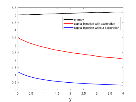
Figure 1: Expected entropy and expected capital injection.

Let us denote some parameters $(\xi^{*},\psi_{1}^{*},\psi_{2}^{*},\psi_{3}^{*},\psi_{4}^{*})$ by

$$\begin{cases}\displaystyle\xi^{*}=\frac{1}{\rho}\left(-\frac{1}{2}\sigma_{Z}^{2}\kappa^{2}+\sqrt{1-\kappa^{2}}\zeta+\frac{\gamma}{2}\ln\left(\frac{(2\pi\gamma)^{d}}{|\sigma\sigma^{\top}|}\right)+\alpha\right),\\[8.99994pt] \displaystyle\psi^{*}_{1}=\mu+\sigma_{z}\sqrt{1-\kappa^{2}}\sigma\eta,\\[5.0pt] \displaystyle\psi_{2}^{*}=\sigma,\\[5.0pt] \displaystyle\psi_{3}^{*}=-\frac{1}{2}\kappa^{2}\sigma_{Z}^{2},\\[5.0pt] \displaystyle\psi_{4}^{*}=\frac{1}{2}\sigma_{Z}^{2}\kappa^{2}-\sqrt{1-\kappa^{2}}\zeta-\frac{\gamma}{2}\ln\left(\frac{(2\pi\gamma)^{d}}{|\sigma\sigma^{\top}|}\right)-\alpha.\end{cases}$$ (5.7)

Using Definition 4.2, the q-function can be expressed by, for all $(y,\tilde{\theta})\in\mathds{R}_{+}\times{\cal A}$,

$$q(y,\tilde{\theta}) =\frac{(\psi_{1}^{*})^{\top}\tilde{\theta}}{1+y}-\frac{\tilde{\theta}^{\top}\psi_{2}^{*}(\psi_{2}^{*})^{\top}\tilde{\theta}}{2(1+y)^{2}}+\frac{\psi_{3}^{*}}{(1+y)^{2}}-\rho\ln(1+y)+\psi_{4}^{*},$$ (5.8)

and the value function $v(y)$ can be written by

$$v(y)=\ln(1+y)+\xi^{*},\quad\forall y\in\mathds{R}_{+}.$$ (5.9)

Based on (5.8)-(5.9), for all $(y,\tilde{\theta})\in\mathds{R}_{+}\times{\cal A}$, we can parameterize the optimal value function and the optimal q-function in the exact form as:

$$\begin{cases}\displaystyle J^{\xi}(y)=\ln(1+y)+\xi,\\[10.00002pt] \displaystyle q^{\bm{\psi}}(y,\tilde{\theta})=\frac{\psi_{1}^{\top}\tilde{\theta}}{1+y}-\frac{\tilde{\theta}^{\top}\psi_{2}\psi_{2}^{\top}\tilde{\theta}^{\top}}{2(1+y)^{2}}+\frac{\psi_{3}}{(1+y)^{2}}-\rho\ln(1+y)+\psi_{4},\end{cases}$$ (5.10)

with the parameters $(\xi,\psi_{1},\psi_{2},\psi_{3},\psi_{4})\in\mathds{R}\times\mathds{R}^{d}\times\mathds{R}^{d\times d}\times\mathds{R}\times\mathds{R}$ to be learnt, and the optimal policy can be parameterized by $\pi^{\bm{\psi}}(\theta\mid y)=\frac{\exp\left\{\frac{1}{\gamma}q^{\bm{\psi}}(y,\theta)\right\}}{\int_{\cal A}\exp\left\{\frac{1}{\gamma}q^{\bm{\psi}}(y,\theta)\right\}d\theta}$. We can verify that the parameterized value function and q-function satisfy assumptions (A_ξ) and (A_ψ).

We consider the modek with one risky asset (i.e., $d=1$), and we set the coefficients of the simulator to be $\mu=0.2$, $\sigma=1$, $\sigma_{Z}=0.2$ and $\kappa=0.5$. Furthermore, we set $\gamma=\rho=0.2$ and the truncated horizon $T=12$, the time step $\Delta t=0.008$ and the number of episodes $N=10^{4}$. The learning rates $(\alpha_{\psi},\alpha_{\xi})$ are given by

$$\alpha_{\psi}(i) =\begin{cases}\displaystyle(1,0.0078,0.049,0.01)\times 10^{-2},&1\leq i\leq 3\cdot 10^{3},\\[6.00006pt] \displaystyle(8,0.0415,0.095,0.026)\times 10^{-3},&3\cdot 10^{3}<i\leq 6\cdot 10^{3},\\[6.00006pt] \displaystyle(1,0.003,0.001,0.002)\times 10^{-4},&6\cdot 10^{3}<i\leq 10^{4},\end{cases}$$

and

$$\alpha_{\xi}(i) =\begin{cases}\displaystyle 2.35\times 10^{-4},&1\leq i\leq 3\cdot 10^{3},\\[6.00006pt] \displaystyle 7.5\times 10^{-5},&3\cdot 10^{3}<i\leq 6\cdot 10^{3},\\[6.00006pt] \displaystyle 7\times 10^{-6},&6\cdot 10^{3}<i\leq 10^{4}.\end{cases}$$

Based on Algorithm 1, we plot in Figure 2 the numerical results on the convergence of iterations for parameters $(\psi_{1},\psi_{2},\psi_{3},\psi_{4},\xi)$ in the optimal value function and the optimal q-function. The learnt parameters for the optimal value function and the optimal q-function are summarized in Table 1 .

Table 1: The true value and learnt value of the parameters $(\psi_{1},\psi_{2},\psi_{3},\psi_{4},\xi)$.

	$\psi_{1}$	$\psi_{2}$	$\psi_{3}$	$\psi_{4}$	$\xi$
True value	0.3732	1.0000	-0.0050	-0.0725	0.3624
Learnt value	0.3726	1.0025	-0.0114	-0.0725	0.3593

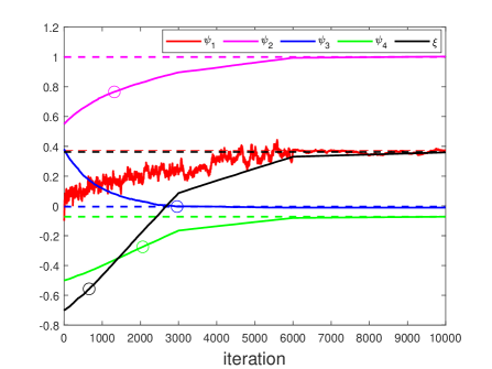
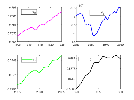
Figure 2: Convergence of parameter iterations in the optimal value function and the optimal q-function using Algorithm 1. (a): paths of learnt parameters for the optimal value function and the optimal q-function vs optimal parameters shown in the dashed line; (b): “zoom-in” paths of learnt parameters for the hollow circles selected in panel (a) to illustrate the fluctuations of the local path; (c): the learnt value function vs the optimal value function.

6 Proofs

This section collects all proofs of the main results presented in previous sections.

Proof of Lemma 3.1.

We can deduce from (3.6) and (3.9) that, for all $(x,z)\in\mathds{R}_{+}\times(0,\infty)$,

$$\hat{\rm w}(x,z) =\sup_{\theta\in\mathbb{U}^{r}}\mathbb{E}\left[-\int_{0}^{\infty}e^{-\rho s}dL_{s}^{X}\big{|}X_{0}=x,Z_{0}=z\right]$$

$$=\sup_{\tilde{\theta}\in\tilde{\mathbb{U}}^{r}}\mathbb{E}\left[-Z_{0}\int_{0}^{\infty}e^{-\rho s}\frac{Z_{s}}{Z_{0}}dL_{s}^{Y}\big{|}X_{0}=x,Z_{0}=z\right]$$

$$=z\sup_{\tilde{\theta}\in\tilde{\mathbb{U}}^{r}}\mathbb{E}^{\mathbb{Q}^{W}}\left[-\int_{0}^{\infty}e^{-\rho s}dL_{s}^{Y}\big{|}X_{0}=x,Y_{0}=\frac{x}{z}\right]$$

$$=zu\left(\frac{x}{z}\right),$$

where we recall that $L^{Y}=(L_{t}^{Y})_{t\geq 0}$ is the local time process associated with the process $Y=(Y_{t})_{t\geq 0}$ at the reflecting boundary $0$ (c.f. Eq. (3.7)). This proves the lemma. ∎

Proof of Theorem 3.2.

Note that the optimal feedback control function $y\to\tilde{\theta}^{*}(y)$ given by (3.16) satisfies the Lipschitz continuous and linear growth conditions. Hence, the SDE (3.17) satisfied by $Y^{*}$ admits a unique strong solution, which gives that $\tilde{\theta}^{*}\in\tilde{\mathbb{U}}^{\rm r}$. Next, it follows from (3.14) that $|u(y)|\leq\frac{1-\gamma}{\gamma}$ for all $y\in\mathds{R}_{+}$. This yields the transversality condition that

$$\lim_{T\to\infty}\mathbb{E}^{\mathbb{Q}^{W}}\left[e^{-\rho T}u(Y_{T})\right]=0.$$ (6.1)

Fix $(T,y)\in(0,\infty)\times\mathds{R}_{+}$ and $\tilde{\theta}\in\tilde{\mathbb{U}}^{\rm r}$. By applying Itô’s formula to $e^{-\rho T}u(Y_{T})$, we arrive at

$$e^{-\rho T}u(Y_{T})=u(y)+\int_{0}^{T}e^{-\rho s}u^{\prime}(Y_{s})\tilde{\theta}_{s}^{\top}\sigma dW_{s}+\int_{0}^{T}e^{-\rho s}\sigma_{Z}(Y_{s}+1)u^{\prime}(Y_{s})d\tilde{W}^{\kappa}_{s}$$

$$\qquad+\int_{0}^{T}e^{-\rho s}u^{\prime}(Y_{s})dL_{s}^{Y}+\int_{0}^{T}e^{-\rho s}({\cal L}^{\tilde{\theta}_{s}}u-\rho u)(Y_{s})ds,$$ (6.2)

where, for any $\tilde{\theta}\in\mathds{R}^{d}$, the operator ${\cal L}^{\tilde{\theta}}$ acting on $C^{2}(\mathds{R}_{+})$ is defined by

$${\cal L}^{\tilde{\theta}}g(y) :=\tilde{\theta}^{\top}\mu g^{\prime}(y)+\frac{1}{2}\tilde{\theta}^{\top}\sigma\sigma^{\top}\tilde{\theta}g^{\prime\prime}(y)-\sqrt{1-\kappa^{2}}\sigma_{Z}(y+1)\tilde{\theta}^{\top}\sigma\eta g^{\prime\prime}(y)+\frac{1}{2}\sigma_{Z}^{2}(y+1)^{2}g^{\prime\prime}(y),\quad\forall y\in\mathds{R}_{+}.$$

Taking the expectation on both sides of (6), we deduce from the Neumann boundary condition $u^{\prime}(0)=1$ that

$$\mathbb{E}^{\mathbb{Q}^{W}}\left[-\int_{0}^{T}e^{-\rho s}dL_{s}^{Y}\right] =u(y)-\mathbb{E}^{\mathbb{Q}^{W}}\left[e^{-\rho T}u(Y_{T})\right]+\mathbb{E}^{\mathbb{Q}^{W}}\left[\int_{0}^{T}e^{-\rho s}({\cal L}^{\tilde{\theta}_{s}}u-\rho u)(Y_{s})ds\right]$$

$$\leq u(y)-\mathbb{E}^{\mathbb{Q}^{W}}\left[e^{-\rho T}u\left(Y_{T}\right)\right].$$ (6.3)

Here, the last inequality in (6) holds because of $({\cal L}^{\tilde{\theta}}u-\rho u)(y)\leq 0$ for all $y\in\mathds{R}_{+}$ and $\tilde{\theta}\in\mathds{R}^{d}$. Letting $T\to\infty$ in (6), we obtain from (6.25) and DCT that, for all $\tilde{\theta}\in\tilde{\mathbb{U}}^{\rm r}$,

$$\mathbb{E}^{\mathbb{Q}^{W}}\left[-\int_{0}^{\infty}e^{-\rho s}dL_{s}^{Y}\right]\leq u(y),\quad\forall y\in\mathds{R}_{+},$$

where the equality holds when $\tilde{\theta}=\tilde{\theta}^{*}$, and the proof of the theorem is completed. ∎

Proof of Theorem 4.1.

We first prove item (i). For $T>0$ and $y\in\mathds{R}_{+}$, applying Itô’s formula to the process $e^{-\rho t}J(\tilde{Y}_{t}^{{\bm{\pi}}^{\prime}};\bm{\pi})$ from $0$ to $T$, we can obtain that

$$e^{-\rho T}J(\tilde{Y}_{T}^{{\bm{\pi}}^{\prime}};\bm{\pi})-J(y;\bm{\pi})-\int_{0}^{T}e^{-\rho t}dL_{t}^{\bm{\pi}^{\prime}}-\gamma\int_{0}^{T}\int_{\cal A}e^{-\rho t}\ln\left(\bm{\pi}^{\prime}(\tilde{\theta};\tilde{Y}_{t}^{{\bm{\pi}}^{\prime}})\right)\bm{\pi}^{\prime}(\tilde{\theta};\tilde{Y}_{t}^{{\bm{\pi}}^{\prime}})d\tilde{\theta}dt$$

$$=\int_{0}^{T}e^{-\rho t}\int_{\cal A}\left(\left[H\left(\tilde{\theta},J_{y}(\tilde{Y}_{t}^{{\bm{\pi}}^{\prime}};\bm{\pi}),J_{yy}(\tilde{Y}_{t}^{{\bm{\pi}}^{\prime}};\bm{\pi})\right)-\rho J(\tilde{Y}_{t}^{{\bm{\pi}}^{\prime}};\bm{\pi})\right]+\frac{\sigma_{Z}^{2}(\tilde{Y}_{t}^{{\bm{\pi}}^{\prime}}+1)^{2}}{2}J_{yy}(\tilde{Y}_{t}^{{\bm{\pi}}^{\prime}};\bm{\pi})\right.$$

$$\quad\left.-\gamma\ln\bm{\pi}^{\prime}(\tilde{\theta};\tilde{Y}_{t}^{{\bm{\pi}}^{\prime}})\right)\bm{\pi}^{\prime}(\tilde{\theta};\tilde{Y}_{t}^{{\bm{\pi}}^{\prime}})d\tilde{\theta}dt+\int_{0}^{T}e^{-\rho t}\left(J_{y}(\tilde{Y}_{t}^{{\bm{\pi}}^{\prime}};\bm{\pi})-1\right)dL_{t}^{\bm{\pi}^{\prime}}$$

$$\quad+\int_{0}^{T}e^{-\rho t}\tilde{\sigma}(\tilde{Y}_{t}^{{\bm{\pi}}^{\prime}},\bm{\pi}^{\prime}(\cdot\mid\tilde{Y}_{t}^{{\bm{\pi}}^{\prime}}))J_{y}(\tilde{Y}_{t}^{{\bm{\pi}}^{\prime}};\bm{\pi})dB_{t}.$$ (6.4)

As $J(\cdot;\bm{\pi})\in C^{2}(\mathds{R}_{+})$ satisfies the PDE (4.6), we can see that

$$\int_{0}^{T}e^{-\rho t}\left(J_{y}(\tilde{Y}_{t}^{{\bm{\bm{\pi}}}^{\prime}};\bm{\bm{\pi}})-1\right)dL_{t}^{\bm{\bm{\pi}}^{\prime}}=\int_{0}^{T}e^{-\rho t}\left(J_{y}(0;\bm{\bm{\pi}})-1\right)dL_{t}^{\bm{\bm{\pi}}^{\prime}}=0.$$ (6.5)

Moreover, it follows from Lemma 2 in Jia and Zhou (2023) that, $\forall y\in\mathds{R}_{+}$,

$$\int_{\cal A}\left(\left[H\left(\tilde{\theta},J_{y}(y;\bm{\pi}),J_{yy}(y;\bm{\pi})\right)-\rho J(y;\bm{\pi})\right]+\frac{\sigma_{Z}^{2}(y+1)^{2}}{2}J_{yy}(y;\bm{\pi})-\gamma\ln\bm{\pi}^{\prime}(\tilde{\theta};y)\right)\bm{\pi}^{\prime}(\tilde{\theta};y)d\tilde{\theta}$$ (6.6)

$$\geq\int_{\cal A}\left(\left[H\left(\tilde{\theta},J_{y}(y;\bm{\pi}),J_{yy}(y;\bm{\pi})\right)-\rho J(y;\bm{\pi})\right]+\frac{\sigma_{Z}^{2}(y+1)^{2}}{2}J_{yy}(y;\bm{\pi})-\gamma\ln\bm{\pi}(\tilde{\theta};y)\right)\bm{\pi}(\tilde{\theta};y)d\tilde{\theta}=0.$$

From (6), (6.5) and (6.6), we deduce that

$$e^{-\rho T}J(\tilde{Y}_{T}^{{\bm{\pi}}^{\prime}};\bm{\pi})-J(y;\bm{\pi})-\int_{0}^{T}e^{-\rho t}dL_{t}^{\bm{\pi}^{\prime}}-\gamma\int_{0}^{T}\int_{\cal A}e^{-\rho t}\ln\left(\bm{\pi}^{\prime}(\tilde{\theta};\tilde{Y}_{t}^{{\bm{\pi}}^{\prime}})\right)\bm{\pi}^{\prime}(\tilde{\theta};\tilde{Y}_{t}^{{\bm{\pi}}^{\prime}})d\tilde{\theta}dt$$

$$\qquad\geq\int_{0}^{T}e^{-\rho t}\tilde{\sigma}(\tilde{Y}_{t}^{{\bm{\pi}}^{\prime}},\bm{\pi}^{\prime}(\cdot\mid\tilde{Y}_{t}^{{\bm{\pi}}^{\prime}}))J_{y}(\tilde{Y}_{t}^{{\bm{\pi}}^{\prime}};\bm{\pi})dB_{t}.$$ (6.7)

Taking the expectation on both side of (6) and letting $T\to\infty$, by (4.17) and the monotone convergence theorem (MCT), we conclude that for any $y\in\mathds{R}_{+}$,

$$J(y;\bm{\pi}) \leq-\lim_{T\to\infty}\mathbb{E}^{\mathbb{Q}^{W}}\left[\int_{0}^{T}e^{-\rho t}dL_{t}^{\bm{\pi}^{\prime}}\right]-\gamma\lim_{T\to\infty}\mathbb{E}^{\mathbb{Q}^{W}}\left[\int_{0}^{T}\int_{\cal A}e^{-\rho t}\ln\left(\bm{\pi}^{\prime}(\tilde{\theta};\tilde{Y}_{t}^{{\bm{\pi}}^{\prime}})\right)\bm{\pi}^{\prime}(\tilde{\theta};\tilde{Y}_{t}^{{\bm{\pi}}^{\prime}})d\tilde{\theta}dt\right]$$

$$\qquad+\lim_{T\to\infty}\mathbb{E}^{\mathbb{Q}^{W}}\left[e^{-\rho T}J(\tilde{Y}_{T}^{{\bm{\pi}}^{\prime}};\bm{\pi})\right]$$

$$=\mathbb{E}^{\mathbb{Q}^{W}}\left[-\int_{0}^{\infty}e^{-\rho t}dL_{t}^{\bm{\pi}^{\prime}}-\gamma\int_{0}^{\infty}\int_{\cal A}e^{-\rho t}\ln\left(\bm{\pi}^{\prime}(\tilde{\theta};\tilde{Y}_{t}^{{\bm{\pi}}^{\prime}})\right)\bm{\pi}^{\prime}(\tilde{\theta};\tilde{Y}_{t}^{{\bm{\pi}}^{\prime}})d\tilde{\theta}dt\right]$$

$$=J(y;\bm{\pi}^{\prime}).$$

Next we deal with item (ii). Denote by $J^{*}(y)=J(y;\bm{\pi}^{*})$. Thus, $J^{*}(y)$ satisfies Eq. (4.6), and Lemma 2 in Jia and Zhou (2023) shows that

$$\int_{\cal A}\left(\left[H\left(\tilde{\theta},y,J_{y}^{*}(y),J_{yy}^{*}(y)\right)-\rho J^{*}(y)\right]+\frac{\sigma_{Z}^{2}(y+1)^{2}}{2}J_{yy}^{*}(y)-\gamma\ln\bm{\pi}^{*}(\tilde{\theta};y)\right)\bm{\pi}^{*}(\tilde{\theta};y)d\tilde{\theta}$$

$$=\sup_{\bm{\pi}\in{\mathcal{P}}({\mathcal{A}})}\int_{\cal A}\left(\left[H\left(\tilde{\theta},y,J_{y}^{*}(y),J_{yy}^{*}(y)\right)-\rho J^{*}(y)\right]+\frac{\sigma_{Z}^{2}(y+1)^{2}}{2}J^{*}_{yy}(y)-\gamma\ln\bm{\pi}(\tilde{\theta};y)\right)\bm{\pi}(\tilde{\theta};y)d\tilde{\theta}=0.$$

Fix $(T,y)\in(0,\infty)\times\mathds{R}_{+}$ and $\bm{\pi}\in\Pi$. By applying Itô’s formula to $e^{-\rho T}J^{*}(\tilde{Y}_{T}^{\bm{\pi}^{*}})$, we arrive at

$$e^{-\rho T}J^{*}(\tilde{Y}_{T}^{\bm{\pi}}) =J^{*}(y)++\int_{0}^{T}e^{-\rho s}J^{*}_{y}(\tilde{Y}_{s}^{\bm{\pi}})dL_{s}^{Y}+\int_{0}^{T}e^{-\rho s}({\cal L}^{\bm{\pi}(\cdot|\tilde{Y}_{s}^{\bm{\pi}})}J^{*}-\rho J^{*})(\tilde{Y}_{s}^{\bm{\pi}})ds$$

$$\quad+\int_{0}^{T}e^{-\rho s}J^{*}_{y}(\tilde{Y}_{s}^{\bm{\pi}})\tilde{\sigma}(\tilde{Y}_{s}^{\bm{\pi}},\bm{\pi}(\cdot|\tilde{Y}_{s}^{\bm{\pi}}))dB_{s},$$ (6.8)

where, for any $\bm{\pi}\in\Pi$, the operator ${\cal L}^{\bm{\pi}}$ acting on $C^{2}(\mathds{R}_{+})$ is defined by

$${\cal L}^{\bm{\pi}}g(y) :=\tilde{b}(y,\bm{\pi})g^{\prime}(y)+\frac{1}{2}\tilde{\sigma}(y,\bm{\pi})g^{\prime\prime}(y),\quad\forall y\in\mathds{R}_{+}.$$

Taking the expectation on both sides of (6), we deduce from the Neumann boundary condition $J^{*}_{y}(0)=1$ that

$$\mathbb{E}^{\mathbb{Q}^{W}}\left[-\int_{0}^{T}e^{-\rho s}dL_{s}^{Y}\right] =J^{*}(y)-\mathbb{E}^{\mathbb{Q}^{W}}\left[e^{-\rho T}v(\tilde{Y}_{T}^{\bm{\pi}})\right]+\mathbb{E}^{\mathbb{Q}^{W}}\left[\int_{0}^{T}e^{-\rho s}({\cal L}^{\bm{\pi}(\cdot|\tilde{Y}_{s}^{\bm{\pi}})}v-\rho v)(\tilde{Y}_{s})ds\right]$$

$$\leq J^{*}(y)-\mathbb{E}^{\mathbb{Q}^{W}}\left[e^{-\rho T}J^{*}\left(\tilde{Y}_{T}^{\bm{\pi}}\right)\right].$$ (6.9)

Here, the last inequality in (6) holds true due to $({\cal L}^{\bm{\pi}}v-\rho v)(y)\leq 0$ for all $y\in\mathds{R}_{+}$ and $\bm{\pi}\in{\cal P}({\cal A})$. Toward this end, letting $T\to\infty$ in (6), we obtain from (4.11) and MCT that, for all $\bm{\pi}\in\Pi$,

$$\mathbb{E}^{\mathbb{Q}^{W}}\left[-\int_{0}^{\infty}e^{-\rho s}dL_{s}^{Y}\right]\leq v(y),\quad\forall y\in\mathds{R}_{+},$$

where the equality holds when $\bm{\pi}=\bm{\pi}^{*}$. This implies that $J^{*}(y)=v(y)$ is the optimal value function and $\bm{\pi}^{*}$ is the optimal policy.

Next, we move to item (iii). To find the fix point, we use the iteration method and start with a special Gaussian policy: $\bm{\pi}_{0}(\cdot|y)\sim\mathcal{N}\left(\cdot\leavevmode\nobreak\ |c_{1}(1+y),c_{2}(1+y)^{2}\right)$, with vector $c_{1}\in\mathds{R}^{d}$ and positive matrix $c_{2}\in\mathds{R}^{d\times d}$. Then it follows that the resulting value function $J^{\bm{\pi}_{0}}(y)$ satisfies the equation:

$$\begin{cases}\displaystyle\int_{\mathcal{A}}\left[H(\theta,y,J^{\bm{\pi}_{0}}_{y}(y),J^{\bm{\pi}_{0}}_{yy}(y))-\gamma\log\bm{\pi}_{0}(\theta|y)\right]\bm{\pi}_{0}(\theta|y)d\theta+\frac{\sigma_{Z}^{2}}{2}(y+1)^{2}J^{\bm{\pi}_{0}}_{yy}(y)=\rho J^{\bm{\pi}_{0}}(y),\\[11.99998pt] \displaystyle J^{\bm{\pi}_{0}}_{y}(y)=1.\end{cases}$$ (6.10)

By standard arguments, we can show that the classical solution of (6.10) is given by

$$J^{\bm{\pi}_{0}}(y)=\ln(1+y)+C,\quad\forall y\in\mathds{R}_{+}$$

where $C$ is a constant defined by

$$C:=\frac{1}{\rho}\left(\mu^{\top}c_{1}+\sqrt{1-\kappa^{2}}\sigma_{Z}c_{1}^{\top}\sigma\eta-\frac{1}{2}c_{1}^{\top}\sigma\sigma^{\top}c_{1}-\frac{1}{2}\text{tr}(\sigma\sigma^{\top}c_{2})-\frac{1}{2}\sigma_{Z}^{2}+\frac{1}{2}\gamma\ln\left((2\pi)^{d}|c_{2}|\right)+\frac{d}{2}\gamma\right),$$

and for a matrix $A\in\mathds{R}^{d\times d}$, we denote $|A|:=\text{det}(A)$.

Then, using once iteration, we get that

$$\bm{\pi}_{1}(\cdot|y)={\cal I}(\bm{\pi}_{0})\sim\mathcal{N}\left(\cdot\leavevmode\nobreak\ \Big{|}(\sigma\sigma^{\top})^{-1}(\mu+\sigma_{z}\sqrt{1-\kappa^{2}}\sigma\eta)(1+y),(\sigma\sigma^{\top})^{-1}\gamma(1+y)^{2}\right).$$ (6.11)

Again, we can calculate the corresponding reward function as

$$J^{\pi_{1}}(y)=\ln(1+y)+\frac{1}{\rho}\left(-\frac{1}{2}\sigma_{Z}^{2}\kappa^{2}+\sqrt{1-\kappa^{2}}\zeta+\frac{\gamma}{2}\ln\left(\frac{(2\pi\gamma)^{d}}{|\sigma\sigma^{\top}|}\right)+\alpha\right)$$ (6.12)

Then the iteration is applicable again, which yields the improved policy $\bm{\pi}_{2}$ as exactly the Gaussian policy $\bm{\pi}_{1}$ given in (6.11), together with the reward function in (6.12). Then we find that ${\bm{\pi}}^{*}$ give in (4.12) is a fixed point of ${\cal I}$. Thus, we complete the proof. ∎

Proof of Proposition 4.2.

For $T>0$ and $y\in\mathds{R}_{+}$, applying Itô’s formula to the process $e^{-\rho s}J(Y_{s}^{\bm{\pi}};{\bm{\pi}})$ from $0$ to $t$, we can obtain that

$$e^{-\rho s}J(Y_{s}^{{\bm{\pi}}};{\bm{\pi}})-J(y;{\bm{\pi}})-\int_{0}^{t}e^{-\rho s}\hat{q}\left(Y_{s}^{{\bm{\pi}}},\tilde{\theta}_{s}^{{\bm{\pi}}}\right)ds-\int_{0}^{t}e^{-\rho s}dL_{s}^{{\bm{\pi}}}$$

$$=\int_{0}^{t}e^{-\rho s}\left(H\left(\tilde{\theta}^{{\bm{\pi}}},Y_{s}^{{\bm{\pi}}},J_{y}(Y_{s}^{{\bm{\pi}}};{\bm{\pi}}),J_{yy}(Y_{s}^{{\bm{\pi}}};{\bm{\pi}})\right)-\rho J(Y_{s}^{{\bm{\pi}}};{\bm{\pi}})+\frac{\sigma_{Z}^{2}(Y_{s}^{{\bm{\pi}}}+1)^{2}}{2}J_{yy}(Y_{s}^{{\bm{\pi}}};{\bm{\pi}})\right)ds$$

$$\quad+\int_{0}^{t}e^{-\rho t}\left(J_{y}(Y_{s}^{{\bm{\pi}}};{\bm{\pi}})-1\right)dL_{s}^{{\bm{\pi}}}+\int_{0}^{t}e^{-\rho s}(\tilde{\theta}^{{\bm{\pi}}})^{\top}\sigma J_{y}(Y_{s}^{{\bm{\pi}}};{\bm{\pi}})dW_{s}$$

$$\quad-\int_{0}^{t}e^{-\rho s}\sigma_{Z}(Y_{s}^{{\bm{\pi}}}+1)J_{y}(Y_{s}^{{\bm{\pi}}};{\bm{\pi}})d\tilde{W}^{\kappa}_{s}$$

$$=\int_{0}^{t}e^{-\rho s}\left(q(Y_{s}^{{\bm{\pi}}},\tilde{\theta}^{{\bm{\pi}}};{\bm{\pi}})-\hat{q}\left(Y_{s}^{{\bm{\pi}}},\tilde{\theta}_{s}^{{\bm{\pi}}}\right)\right)ds+\int_{0}^{t}e^{-\rho s}(\tilde{\theta}^{{\bm{\pi}}})^{\top}\sigma J_{y}(Y_{s}^{{\bm{\pi}}};{\bm{\pi}})dW_{s}$$

$$\quad-\int_{0}^{t}e^{-\rho s}\sigma_{Z}(Y_{s}^{{\bm{\pi}}}+1)J_{y}(Y_{s}^{{\bm{\pi}}};{\bm{\pi}})d\tilde{W}^{\kappa}_{s}.$$ (6.13)

From Eq. (6), we can see that, if $\hat{q}(y,\tilde{\theta})=q(y,\tilde{\theta};{\bm{\pi}})$ for all $(y,\tilde{\theta})\in\mathds{R}_{+}\times{\cal A}$, then the above process, and hence the process defined by (4.14) is an $((\mathcal{F}_{t})_{t\geq 0},\mathbb{Q})$-martingale.

On the other hand, if the process (4.14) is an $((\mathcal{F}_{t})_{t\geq 0},\mathbb{Q})$-martingale, let us next show that $\hat{q}(y,\tilde{\theta})=q(y,\tilde{\theta};{\bm{\pi}})$ for all $(y,\tilde{\theta})\in\mathds{R}_{+}\times{\cal A}$. By (6) we can see that the process

$$\left\{\int_{0}^{t}e^{-\rho s}\left(q(Y_{s}^{{\bm{\pi}}},\tilde{\theta}^{{\bm{\pi}}};{\bm{\pi}})-\hat{q}\left(Y_{s}^{{\bm{\pi}}},\tilde{\theta}_{s}^{{\bm{\pi}}}\right)\right)ds\right\}_{t\geq 0}$$

is a continuous local martingale with finite variation and hence zero quadratic variation. Hence, it follows that $\int_{0}^{t}e^{-\tilde{\rho}s}(q(Y_{s}^{{\bm{\pi}}},\tilde{\theta}^{{\bm{\pi}}};{\bm{\pi}})-\hat{q}(Y_{s}^{{\bm{\pi}}},\tilde{\theta}_{s}^{{\bm{\pi}}}))ds=0$ for all $t\in[0,\infty)$, $\mathbb{Q}$-a.s. (see Chapter 1, Exercise 5.21 in Karatzas and Shreve (2014)). For $y\in\mathds{R}_{+},a\in{\cal A}$, denote by $h(y,\tilde{\theta})=q(y,\tilde{\theta};{\bm{\pi}})-\hat{q}(y,\tilde{\theta})$, which is a continuous function that maps $\mathds{R}_{+}\times\mathcal{A}$ to $\mathds{R}_{+}$. Next we argue by contradiction. Suppose there exists a pair $(y_{0},\tilde{\theta}_{0})\in\mathds{R}_{+}\times{\cal A}$ and $\epsilon>0$ such that $h(y_{0},\tilde{\theta}_{0})>\epsilon$. By the continuity of $h$, there exists $\delta>0$ such that $h(y,\tilde{\theta})>\epsilon/2$ for all $(y,\tilde{\theta})$ with $\max\{|y-y_{0}|,|\tilde{\theta}-\tilde{\theta}_{0}|\}<\delta$.

Now consider the state process, still denoted by $Y^{\bm{\pi}}$, starting from $(y_{0},\tilde{\theta}_{0})$, namely, $(Y_{t}^{\bm{\pi}})_{t\geq 0}$ follows (6) with $Y^{\bm{\pi}}_{0}=y_{0}$ and $\tilde{\theta}_{0}^{\bm{\pi}}=\tilde{\theta}_{0}$. Define the stopping time $\tau$ by

$$\tau:=\inf\left\{t\geq 0:\left|Y_{t}^{\bm{\pi}}-y_{0}\right|>\delta\right\}.$$

We have already shown that there exists $\Omega_{0}\in\mathcal{F}$ with $\mathbb{Q}\left(\Omega_{0}\right)=0$ such that for all $\omega\in\Omega\backslash\Omega_{0}$, $\int_{0}^{t}e^{-\rho s}(q(Y_{s}^{{\bm{\pi}}},\tilde{\theta}^{{\bm{\pi}}};{\bm{\pi}})-\hat{q}(Y_{s}^{{\bm{\pi}}},\tilde{\theta}_{s}^{{\bm{\pi}}}))ds=0$ for all $t\in[0,\infty)$. It follows from Lebesgue’s differentiation theorem that for any $\omega\in\Omega\backslash\Omega_{0}$,

$$h\left(Y_{t}^{\bm{\pi}}(\omega),\tilde{\theta}_{t}^{\bm{\pi}}(\omega)\right)=0,\leavevmode\nobreak\ \text{a.e., for }\leavevmode\nobreak\ t\in[0,\tau(\omega)].$$

Consider the set ${\cal O}(\omega)=\{t\in[0,\tau(\omega)]:|\tilde{\theta}_{t}^{\bm{\pi}}(\omega)-\tilde{\theta}_{0}|<\delta\}\subset[0,\tau(\omega)]$. Because $h(Y_{t}^{\bm{\pi}}(\omega),\tilde{\theta}_{t}^{\bm{\pi}}(\omega))>\frac{\epsilon}{2}$ when $t\in{\cal O}(\omega)$, we conclude that ${\cal O}(\omega)$ has Lebesgue measure zero for any $\omega\in\Omega\backslash\Omega_{0}$. That is

$$\int_{0}^{\infty}{\bf 1}_{\{t\leq\tau(\omega)\}}{\bf 1}_{\left\{|\tilde{\theta}_{t}^{\bm{\pi}}(\omega)-\tilde{\theta}_{0}|<\delta\right\}}dt=0.$$

Integrating $\omega$ with respect to $\mathbb{Q}$ and applying Fubini’s theorem, we obtain that

$$0 =\int_{\Omega}\int_{0}^{\infty}{\bf 1}_{\{t\leq\tau(\omega)\}}{\bf 1}_{\left\{|\tilde{\theta}_{t}^{\bm{\pi}}(\omega)-\tilde{\theta}_{0}|<\delta\right\}}dt\mathbb{Q}(d\omega)\int_{0}^{\infty}\mathbb{E}^{\mathbb{Q}}\left[{\bf 1}_{\{t\leq\tau\}}{\bf 1}_{\left\{|\tilde{\theta}_{t}^{\bm{\pi}}-\tilde{\theta}_{0}|<\delta\right\}}\right]dt$$

$$=\int_{0}^{\infty}\mathbb{E}\left[{\bf 1}_{\{t\leq\tau\}}\mathbb{Q}^{\mathbb{Q}}\left(|\tilde{\theta}_{t}^{\bm{\pi}}-\tilde{\theta}_{0}|<\delta|\mathcal{F}_{t}\right)\right]dt=\int_{0}^{\infty}\mathbb{E}\left[{\bf 1}_{\{t\leq\tau\}}\int_{|\tilde{\theta}-\tilde{\theta}_{0}|<\delta}{\bm{\pi}}\left(\tilde{\theta}|Y_{t}^{{\bm{\pi}}}\right)d\tilde{\theta}\right]dt$$

$$\geq\min_{\left|y-y_{0}\right|<\delta}\left\{\int_{|\tilde{\theta}-\tilde{\theta}_{0}|<\delta}{\bm{\pi}}\left(\tilde{\theta}|y\right)d\tilde{\theta}\right\}\int_{0}^{\infty}\mathbb{E}^{\mathbb{Q}}\left[{\bf 1}_{\{t\leq\tau\}}\right]dt$$

$$=\min_{\left|y-y_{0}\right|<\delta}\left\{\int_{|\tilde{\theta}-\tilde{\theta}_{0}|<\delta}{\bm{\pi}}\left(\tilde{\theta}|y\right)d\tilde{\theta}\right\}\mathbb{E}^{\mathbb{Q}}[\tau]\geq 0.$$

The above implies that $\min_{|y-y_{0}|<\delta}\{\int_{|\tilde{\theta}-\tilde{\theta}_{0}|<\delta}{\bm{\pi}}(\tilde{\theta}|y)d\tilde{\theta}\}=0$ . However, this contradicts Definition 4.1 about an admissible policy. Indeed, Definition 4.1-(i) stipulates $\operatorname{supp}{\bm{\pi}}(\cdot|y)=\mathcal{A}$ for any $y\in\mathds{R}_{+}$; hence $\int_{|\tilde{\theta}-\tilde{\theta}_{0}|<\delta}{\bm{\pi}}(\tilde{\theta}|y)d\tilde{\theta}>0$. Then the continuity in Definition 4.1-(iii) yields $\min_{|y-y_{0}|<\delta}\{\int_{|\tilde{\theta}-\tilde{\theta}_{0}|<\delta}{\bm{\pi}}(\tilde{\theta}|y)d\tilde{\theta}\}>0$, which is a contradiction. Hence we conclude that $q(y,\tilde{\theta};{\bm{\pi}})=\hat{q}(y,\tilde{\theta})$ for every $(y,\tilde{\theta})\in\mathds{R}_{+}\times{\cal A}$. ∎

Proof of Theorem 4.3.

If $\hat{J}$ and $\hat{q}$ are respectively the value function and the $q$-function associated with the policy ${\bm{\pi}}$, it follows from the same argument as in the proof of Proposition 4.2 that

$$e^{-\rho t}\hat{J}(Y_{t}^{\bm{\pi}})-\int_{0}^{t}e^{-\rho s}\hat{q}\left(Y_{s}^{\bm{\pi}},\tilde{\theta}_{s}^{\bm{\pi}}\right)ds-\int_{0}^{t}e^{-\rho s}dL_{s}^{\bm{\pi}}$$

is an $((\mathcal{F}_{t})_{t\geq 0},\mathbb{Q})$-martingale.

On the other hand, assume that $e^{-\rho t}\hat{J}(Y_{t}^{{\bm{\pi}}})-\int_{0}^{t}e^{-\rho s}\hat{q}(Y_{s}^{{\bm{\pi}}},\tilde{\theta}_{s}^{{\bm{\pi}}})ds-\int_{0}^{t}e^{-\rho s}dL_{s}^{{\bm{\pi}}}$ is an $((\mathcal{F}_{t})_{t\geq 0},\mathbb{Q})$ martingale. It then holds that, for any $T>0$,

$$\hat{J}(y)=\mathbb{E}^{\mathbb{Q}}\left[e^{-\rho T}\hat{J}(Y_{T}^{\bm{\pi}})-\int_{0}^{T}e^{-\rho s}\hat{q}\left(Y_{s}^{\bm{\pi}},\tilde{\theta}_{s}^{\bm{\pi}}\right)ds-\int_{0}^{T}e^{-\rho s}dL_{s}^{\bm{\pi}}\right].$$ (6.14)

Integrating over the action randomization with respect to the policy ${\bm{\pi}}$ on the side of Eq. (6.14), we get that

$$\hat{J}(y,{\bm{\pi}})=\mathbb{E}^{\mathbb{Q}^{W}}\left[e^{-\rho T}\hat{J}(\tilde{Y}_{T}^{\bm{\pi}};{\bm{\pi}})-\int_{0}^{T}e^{-\rho s}\int_{\cal A}\hat{q}\left(\tilde{Y}_{s}^{\bm{\pi}},\tilde{\theta}\right){\bm{\pi}}(\tilde{\theta}|\tilde{Y}_{s}^{\bm{\pi}})d\tilde{\theta}ds-\int_{0}^{T}e^{-\rho s}dL_{s}^{\bm{\pi}}\right].$$ (6.15)

In view that $\int_{\mathcal{A}}[\hat{q}(y,\tilde{\theta})-\gamma\ln{\bm{\pi}}(\tilde{\theta}|y)]{\bm{\pi}}(\tilde{\theta}|y)d\tilde{\theta}=0$, we obtain

$$\hat{J}(y)=\mathbb{E}^{\mathbb{Q}^{W}}\left[e^{-\rho T}\hat{J}(\tilde{Y}_{T}^{\bm{\pi}})-\gamma\int_{0}^{T}e^{-\rho s}\int_{\cal A}\ln{\bm{\pi}}(\tilde{\theta}|\tilde{Y}_{s}^{\bm{\pi}}){\bm{\pi}}(\tilde{\theta}|\tilde{Y}_{s}^{\bm{\pi}})d\tilde{\theta}ds-\int_{0}^{T}e^{-\rho s}dL_{s}^{\bm{\pi}}\right].$$ (6.16)

Letting $T$ go to infinity on both side of (6.17), we deduce from MCT and (4.15) that

$$\hat{J}(y) =\mathbb{E}^{\mathbb{Q}^{W}}\left[-\gamma\int_{0}^{\infty}e^{-\rho s}\int_{\cal A}\ln{\bm{\pi}}(\tilde{\theta}|\tilde{Y}_{s}^{\bm{\pi}}){\bm{\pi}}(\tilde{\theta}|\tilde{Y}_{s}^{\bm{\pi}})d\tilde{\theta}ds-\int_{0}^{\infty}e^{-\rho s}dL_{s}^{\bm{\pi}}\right].$$ (6.17)

This yields that $\hat{J}(y)=J(y;{\bm{\pi}})$ for all $y\in\mathds{R}_{+}$ by virtue of (4.6). Furthermore, based on Proposition 4.2, the martingale condition implies that $\hat{q}(y,\tilde{\theta})=q(y,\tilde{\theta};{\bm{\pi}})$ for all $(y,\tilde{\theta})\in\mathds{R}_{+}\times{\cal A}$.

Finally, if ${\bm{\pi}}(\tilde{\theta}|y)=\frac{\exp\{\frac{1}{\gamma}\hat{q}(y,\tilde{\theta})\}}{\int_{\mathcal{A}}\exp\{\frac{1}{\gamma}\hat{q}(y,\tilde{\theta})\}d\tilde{\theta}}$ satisfies the condition (4.17), then ${\bm{\pi}}={\cal I}({\bm{\pi}})$ where $\mathcal{I}$ is the map defined in Theorem 4.1. This in turn implies that ${\bm{\pi}}$ is the optimal policy and $\hat{J}$ is the optimal value function. ∎

Proof of Proposition 4.4.

The “only if” part directly follows from the martingale orthogonality condition (4.21), and we only prove the “if” part. Assume that

$$\mathbb{E}^{\mathbb{Q}}\left[\int_{0}^{\infty}\varsigma_{t}dM_{t}^{\xi,\psi}\right]=0$$ (6.18)

for any $\varsigma$ with $\mathbb{E}^{\mathbb{Q}}[\int_{0}^{\infty}|\varsigma_{t}|^{2}d\left<M\right>_{t}]<\infty$. In view of (4.20), Itô’s formula and Neumann boundary condition $J^{\xi}_{y}(0)=1$, we have that

$$dM_{t}^{\xi,\psi} =e^{-\rho t}dJ^{\xi}\left(Y_{t}^{\bm{\pi}}\right)-\rho e^{-\rho t}J^{\xi}\left(Y_{t}^{\bm{\pi}}\right)dt-e^{-\rho s}q^{\psi}\left(Y_{s}^{\bm{\pi}},\tilde{\theta}_{t}^{\bm{\pi}}\right)dt-e^{-\rho t}dL_{t}^{\bm{\pi}}$$

$$=e^{-\rho t}{\cal L}^{\tilde{\theta}^{\bm{\pi}}_{t}}J^{\xi}(Y_{t}^{{\bm{\pi}}})dt-\rho e^{-\rho t}J^{\xi}\left(Y_{t}^{\bm{\pi}}\right)dt-e^{-\rho t}q^{\psi}\left(Y_{t}^{\bm{\pi}},\tilde{\theta}_{t}^{\bm{\pi}}\right)dt$$

$$\quad+J_{y}^{\xi}\left(Y_{t}^{{\bm{\pi}}}\right)\left((\tilde{\theta}^{\bm{\pi}}_{t})^{\top}\sigma dW_{t}-\sigma_{Z}(Y_{t}^{\bm{\pi}}+1)d\tilde{W}^{\kappa}_{t}\right)+e^{-\rho s}(J^{\xi}_{y}(0)-1)dL_{t}^{\bm{\pi}}$$

$$=A_{t}dt+J_{y}^{\xi}\left(Y_{t}^{{\bm{\pi}}}\right)\left((\tilde{\theta}^{\bm{\pi}}_{t})^{\top}\sigma dW_{t}-\sigma_{Z}(Y_{t}^{\bm{\pi}}+1)d\tilde{W}^{\kappa}_{t}\right),$$ (6.19)

where, for any $\tilde{\theta}\in\mathds{R}^{d}$, the operator ${\cal L}^{\tilde{\theta}}$ acting on $C^{2}(\mathds{R}_{+})$ is defined by, for all $y\in\mathds{R}_{+}$,

$${\cal L}^{\tilde{\theta}}g(y) :=\tilde{\theta}^{\top}\mu g^{\prime}(y)+\frac{1}{2}\tilde{\theta}^{\top}\sigma\sigma^{\top}\tilde{\theta}g^{\prime\prime}(y)-\sqrt{1-\kappa^{2}}\sigma_{Z}(y+1)\tilde{\theta}^{\top}\sigma\eta g^{\prime\prime}(y)+\frac{1}{2}\sigma_{Z}^{2}(y+1)^{2}g^{\prime\prime}(y),$$

and the process $A=(A_{t})_{t\geq 0}$ is defined by

$$A_{t}:=e^{-\rho t}{\cal L}^{\tilde{\theta}^{\bm{\pi}}_{t}}J^{\xi}(Y_{t}^{{\bm{\pi}}})-\rho e^{-\rho t}J^{\xi}(Y_{t}^{\bm{\pi}})-e^{-\rho t}q^{\psi}(Y_{t}^{\bm{\pi}},\tilde{\theta}_{t}^{\bm{\pi}}),\leavevmode\nobreak\ t\geq 0.$$

Then, we take the test function $\varsigma_{t}=\mathrm{sgn}(A_{t})$ for $t\geq 0$ and apply the martingale orthogonality condition (6.18) to get that

$$\mathbb{E}^{\mathbb{Q}}\left[\int_{0}^{\infty}\varsigma_{t}dM_{t}^{\xi,\psi}\right]=\mathbb{E}^{\mathbb{Q}}\left[\int_{0}^{\infty}|A_{t}|dt\right]=0.$$

This implies that $A_{t}=0$ almost surely. Thus, the parameterized process $M^{\xi,\psi}$ given by (4.20) is a martingale. ∎

Proof of Theorem 4.5.

We first state the following auxiliary lemma.

Lemma 6.1 (Lemma 8 in Jia and Zhou (2022b)).

Let $f_{h}(x)=f(x)+r_{h}(x)$, where $f$ is a continuous function and $r_{h}$ converges to 0 uniformly on any compact set as $h\rightarrow 0$. Assume that $f_{h}(x_{h}^{*})=0$ and $\lim_{h\rightarrow 0}x_{h}^{*}=x^{*}$. Then $f(x^{*})=0$.

We first apply Lemma 6.1 to prove item (i). We can take $f(x)=\mathbb{E}^{\mathbb{Q}}[\int_{0}^{\infty}\varsigma_{t}dM_{t}^{\xi,\psi}]$ and $f_{h}(x)=\mathbb{E}^{\mathbb{Q}}[\int_{0}^{T}\varsigma_{t}dM_{t}^{\xi,\psi}]$ with $h=1/T$, $x=(\xi,\psi)$. Thus, we need to prove that

$$\mathbb{E}^{\mathbb{Q}}\left[\int_{0}^{\infty}\varsigma_{t}dM_{t}^{\xi,\psi}\right]-\mathbb{E}^{\mathbb{Q}}\left[\int_{0}^{\infty}\varsigma_{t}dM_{t}^{\xi,\psi}\right]=\mathbb{E}^{\mathbb{Q}}\left[\int_{T}^{\infty}\varsigma_{t}dM_{t}^{\xi,\psi}\right]\to 0,$$ (6.20)

as $T\to\infty$ uniformly on any compact subset of $\Theta\times\Psi$. Let ${\cal C}\subset\Theta\times\Psi$ be a compact set, then ${\cal C}$ is a bounded closed set. By the proof of Proposition 4.4 and assumptions (A_ξ) and (A_ψ), we have that

$$\mathbb{E}^{\mathbb{Q}}\left[\int_{T}^{\infty}\varsigma_{t}dM_{t}^{\xi,\psi}\right]$$

$$=\mathbb{E}^{\mathbb{Q}}\left[\int_{T}^{\infty}e^{-\rho t}\varsigma_{t}\left({\cal L}^{\tilde{\theta}^{\bm{\pi}}_{t}}J^{\xi}(Y_{t}^{{\bm{\pi}}})-\rho J^{\xi}(Y_{t}^{\bm{\pi}})-q^{\psi}(Y_{t}^{\bm{\pi}},\tilde{\theta}_{t}^{\bm{\pi}})\right)dt\right]$$

$$=\mathbb{E}^{\mathbb{Q}}\left[\int_{T}^{\infty}e^{-\rho t}\varsigma_{t}\left((\tilde{\theta}^{\bm{\pi}}_{t})^{\top}\mu J_{y}^{\xi}(Y_{t}^{\bm{\pi}})+\frac{1}{2}(\tilde{\theta}^{\bm{\pi}}_{t})^{\top}\sigma\sigma^{\top}\tilde{\theta}^{\bm{\pi}}_{t}J_{yy}^{\xi}(Y_{t}^{\bm{\pi}})-\sqrt{1-\kappa^{2}}\sigma_{Z}(Y_{t}^{\bm{\pi}}+1)(\tilde{\theta}^{\bm{\pi}}_{t})^{\top}\sigma\eta J_{yy}^{\xi}(Y_{t}^{\bm{\pi}})\right.\right.$$

$$\qquad+\left.\left.\frac{1}{2}\sigma_{Z}^{2}(Y_{t}^{\bm{\pi}}+1)^{2}J_{yy}^{\xi}(Y_{t}^{\bm{\pi}})-\rho J^{\xi}(Y_{t}^{\bm{\pi}})-q^{\psi}(Y_{t}^{\bm{\pi}},\tilde{\theta}_{t}^{\bm{\pi}})\right)dt\right]$$

$$\leq(G_{J}(\xi)+G_{q}(\psi))\mathbb{E}^{\mathbb{Q}}\left[\int_{T}^{\infty}e^{-\rho t}\varsigma_{t}\left(\left(\left|(\tilde{\theta}^{\bm{\pi}}_{t})^{\top}\mu\right|+\frac{1}{2}(\tilde{\theta}^{\bm{\pi}}_{t})^{\top}\sigma\sigma^{\top}\tilde{\theta}^{\bm{\pi}}_{t}+\left|\sqrt{1-\kappa^{2}}\sigma_{Z}(Y_{t}^{\bm{\pi}}+1)(\tilde{\theta}^{\bm{\pi}}_{t})^{\top}\sigma\eta\right|\right.\right.\right.$$

$$\qquad+\left.\left.\left.\frac{1}{2}\sigma_{Z}^{2}(Y_{t}^{\bm{\pi}}+1)^{2}+\rho\right)\tilde{J}(Y_{t}^{\bm{\pi}})+\tilde{q}(Y_{t}^{\bm{\pi}},\tilde{\theta}_{t}^{\bm{\pi}})\right)dt\right].$$ (6.21)

This yields that as $T\to\infty$, $\mathbb{E}^{\mathbb{Q}}[\int_{T}^{\infty}\varsigma_{t}dM_{t}^{\xi,\psi}]$ converges to 0 uniformly in $(\xi,\psi)\in{\cal C}$. Then by Lemma 6.1, we get the desired result.

Next we deal with item (ii). By Lemma 6.1, it is sufficient to show that

$$\mathbb{E}^{\mathbb{Q}}\left[\int_{0}^{\infty}\varsigma_{t}dM_{t}^{\xi,\psi}\right]-\mathbb{E}^{\mathbb{Q}}\left[\sum_{k=0}^{K-1}\varsigma_{t_{k}}\left(M_{t_{k+1}}^{\xi,\psi}-M_{t_{k}}^{\xi,\psi}\right)\right]\to 0,$$ (6.22)

as $\Delta t\to\infty$ uniformly on any compact subset of $\Theta\times\Psi$. Let ${\cal C}\subset\Theta\times\Psi$ be a compact set, which is also a bounded closed set. It follows from that

$$\mathbb{E}^{\mathbb{Q}}\left[\int_{0}^{\infty}\varsigma_{t}dM_{t}^{\xi,\psi}\right]-\mathbb{E}^{\mathbb{Q}}\left[\sum_{k=0}^{K-1}\varsigma_{t_{k}}\left(M_{t_{k+1}}^{\xi,\psi}-M_{t_{k}}^{\xi,\psi}\right)\right]$$

$$=\mathbb{E}^{\mathbb{Q}}\left[\int_{0}^{\infty}\varsigma_{t}dM_{t}^{\xi,\psi}\right]-\mathbb{E}^{\mathbb{Q}}\left[\sum_{k=0}^{K-1}\int_{t_{k}}^{t_{k+1}}\varsigma_{t_{k}}dM_{t}^{\xi,\psi}\right]$$

$$=\mathbb{E}^{\mathbb{Q}}\left[\sum_{k=0}^{K-1}\int_{t_{k}}^{t_{k+1}}e^{-\rho t}(\varsigma_{t}-\varsigma_{t_{k}})\left({\cal L}^{\tilde{\theta}^{\bm{\pi}}_{t}}J^{\xi}(Y_{t}^{{\bm{\pi}}})-\rho J^{\xi}(Y_{t}^{\bm{\pi}})-q^{\psi}(Y_{t}^{\bm{\pi}},\tilde{\theta}_{t}^{\bm{\pi}})\right)dt\right]$$

$$\leq\sum_{k=0}^{K-1}\int_{t_{k}}^{t_{k+1}}\mathbb{E}^{\mathbb{Q}}\left[(\varsigma_{t}-\varsigma_{t_{k}})^{2}\right]^{\frac{1}{2}}\mathbb{E}^{\mathbb{Q}}\left[\left({\cal L}^{\tilde{\theta}^{\bm{\pi}}_{t}}J^{\xi}(Y_{t}^{{\bm{\pi}}})-\rho J^{\xi}(Y_{t}^{\bm{\pi}})-q^{\psi}(Y_{t}^{\bm{\pi}},\tilde{\theta}_{t}^{\bm{\pi}})\right)^{2}\right]^{\frac{1}{2}}dt$$

$$\leq\sum_{k=0}^{K-1}\left(\int_{t_{k}}^{t_{k+1}}\mathbb{E}^{\mathbb{Q}}\left[(\varsigma_{t}-\varsigma_{t_{k}})^{2}\right]dt\right)^{\frac{1}{2}}\left(\int_{t_{k}}^{t_{k+1}}\mathbb{E}^{\mathbb{Q}}\left[\left({\cal L}^{\tilde{\theta}^{\bm{\pi}}_{t}}J^{\xi}(Y_{t}^{{\bm{\pi}}})-\rho J^{\xi}(Y_{t}^{\bm{\pi}})-q^{\psi}(Y_{t}^{\bm{\pi}},\tilde{\theta}_{t}^{\bm{\pi}})\right)^{2}\right]dt\right)^{\frac{1}{2}}$$

$$\leq d(\ell(\cdot),\Delta t)\sqrt{\Delta t}\sum_{k=0}^{K-1}\left(\int_{t_{k}}^{t_{k+1}}\mathbb{E}^{\mathbb{Q}}\left[\left({\cal L}^{\tilde{\theta}^{\bm{\pi}}_{t}}J^{\xi}(Y_{t}^{{\bm{\pi}}})-\rho J^{\xi}(Y_{t}^{\bm{\pi}})-q^{\psi}(Y_{t}^{\bm{\pi}},\tilde{\theta}_{t}^{\bm{\pi}})\right)^{2}\right]dt\right)^{\frac{1}{2}}$$

$$\leq d(\ell(\cdot),\Delta t)\sqrt{\Delta t}\sqrt{K}\left(\sum_{k=0}^{K-1}\int_{t_{k}}^{t_{k+1}}\mathbb{E}^{\mathbb{Q}}\left[\left({\cal L}^{\tilde{\theta}^{\bm{\pi}}_{t}}J^{\xi}(Y_{t}^{{\bm{\pi}}})-\rho J^{\xi}(Y_{t}^{\bm{\pi}})-q^{\psi}(Y_{t}^{\bm{\pi}},\tilde{\theta}_{t}^{\bm{\pi}})\right)^{2}\right]dt\right)^{\frac{1}{2}}$$

$$\leq d(\ell(\cdot),\Delta t)\sqrt{T}\left(\mathbb{E}^{\mathbb{Q}}\left[\int_{0}^{T}\left({\cal L}^{\tilde{\theta}^{\bm{\pi}}_{t}}J^{\xi}(Y_{t}^{{\bm{\pi}}})-\rho J^{\xi}(Y_{t}^{\bm{\pi}})-q^{\psi}(Y_{t}^{\bm{\pi}},\tilde{\theta}_{t}^{\bm{\pi}})\right)^{2}dt\right]\right)^{\frac{1}{2}}$$

$$\leq d(\ell(\cdot),\Delta t)\sqrt{T}(G^{2}_{J}(\xi)+G^{2}_{q}(\psi))^{\frac{1}{2}}\mathbb{E}^{\mathbb{Q}}\left[\int_{0}^{T}\left(\left(\left|(\tilde{\theta}^{\bm{\pi}}_{t})^{\top}\mu\right|+\frac{1}{2}(\tilde{\theta}^{\bm{\pi}}_{t})^{\top}\sigma\sigma^{\top}\tilde{\theta}^{\bm{\pi}}_{t}\right.\right.\right.$$

$$\qquad\left.\left.\left.+\left|\sqrt{1-\kappa^{2}}\sigma_{Z}(Y_{t}^{\bm{\pi}}+1)(\tilde{\theta}^{\bm{\pi}}_{t})^{\top}\sigma\eta\right|+\frac{1}{2}\sigma_{Z}^{2}(Y_{t}^{\bm{\pi}}+1)^{2}+\rho\right)\tilde{J}(Y_{t}^{\bm{\pi}})+\tilde{q}(Y_{t}^{\bm{\pi}},\tilde{\theta}_{t}^{\bm{\pi}})\right)^{2}dt\right]^{\frac{1}{2}}$$ (6.23)

where $\ell(t):=\varsigma_{t}$ and $d(\ell(\cdot),\Delta t)=\sup_{|t-s|\leq\Delta t,t,s\in[0,T]}\mathbb{E}^{\mathbb{Q}}[|\ell(t)-\ell(s)|^{2}]^{\frac{1}{2}}$ is the modelus of continuity of $\ell(\cdot)$ in $\mathbb{L}^{2}(\Omega)$. Therefore, $d^{2}(\ell(\cdot),\Delta t)\to 0$ as $\Delta t\to 0$ and we get the desired result (6.22). ∎

Proof of Theorem 5.1.

By Theorem 4.1, it suffices to verify the transversality conditions in (4.11). Note that $y\to v(y)$ is non-decreasing, we have

$$v(y) =\ln(1+y)+\frac{1}{\rho}\left(-\frac{1}{2}\sigma_{Z}^{2}\kappa^{2}+\sqrt{1-\kappa^{2}}\zeta+\frac{\gamma}{2}\ln\left(\frac{(2\pi\gamma)^{d}}{|\sigma\sigma^{\top}|}\right)+\alpha\right)$$

$$\geq\frac{1}{\rho}\left(-\frac{1}{2}\sigma_{Z}^{2}\kappa^{2}+\sqrt{1-\kappa^{2}}\zeta+\frac{\gamma}{2}\ln\left(\frac{(2\pi\gamma)^{d}}{|\sigma\sigma^{\top}|}\right)+\alpha\right).$$

This yields that for any ${\bm{\pi}}\in\Pi$,

$$\limsup_{T\to\infty}\mathbb{E}^{\mathbb{Q}^{W}}\left[e^{-\rho T}v(\tilde{Y}^{\bm{\pi}}_{T})\right]\geq 0.$$ (6.24)

Next, we check the validity of the second transversality condition in (4.11), that is

$$\lim_{T\to\infty}\mathbb{E}^{\mathbb{Q}^{W}}\left[e^{-\rho T}v(Y^{*}_{T})\right]=0.$$ (6.25)

It follows from (4.3) and (5.4) that the controlled state process $Y^{*}=(Y_{t}^{*})_{t\geq 0}$ with policy $\bm{\pi}^{*}$ obeys the following reflected SDE, for all $t\geq 0$,

$$dY_{t}^{*}=(2\alpha+\sqrt{1-\kappa^{2}}\zeta)(1+Y^{*}_{t})dt+\sqrt{\alpha+\frac{d}{2}\gamma+\frac{1}{2}\kappa^{2}\sigma_{Z}^{2}+\sqrt{1-\kappa^{2}}\zeta}(1+Y^{*}_{t})dB_{t}+dL_{t}^{*}.$$

Let us introduce the processes $(H,K)=(H_{t},K_{t})_{t\geq 0}$ by

$$H_{t}:=\ln(1+Y^{*}_{t}),\quad K_{t}:=\int_{0}^{t}\frac{dL_{s}^{*}}{1+Y^{*}_{s}},\quad\forall t\geq 0.$$ (6.26)

Then, $t\to H_{t}$ is a non-negative process wihth $H_{0}=h=\ln(1+y)$. Moreover, $t\to K_{t}$ is a non-decreasing process and satisfies that, a.s.

$$\int_{0}^{t}{\bf 1}_{H_{s}=0}dK_{s}=\int_{0}^{t}{\bf 1}_{Y^{*}_{s}=0}\frac{dL_{s}^{*}}{1+Y^{*}_{s}}=\int_{0}^{t}\frac{dL_{s}^{*}}{1+Y^{*}_{s}}=K_{t},\quad\forall t\geq 0.$$

This implies that $K=(K_{t})_{t\geq 0}$ is the local time of the process $H=(H_{t})_{t\geq 0}$ at the reflecting boundary $0$. By applying Itô’s formula to $H_{t}=\ln(1+Y^{*}_{t})$, we arrive at

$$dH_{t} =\hat{\mu}dt+\hat{\sigma}dB_{t}+\frac{dL_{t}^{*}}{1+Y_{t}^{*}}=\hat{\mu}dt+\hat{\sigma}dB_{t}+dK_{t},\quad t>0,$$ (6.27)

where constants $\hat{\mu}$ and $\hat{\sigma}$ are defined by

$$\hat{\mu} :=2\alpha+\sqrt{1-\kappa^{2}}\zeta-\frac{1}{2}\left(\alpha+\frac{d}{2}\gamma+\frac{1}{2}\kappa^{2}\sigma_{Z}^{2}+\sqrt{1-\kappa^{2}}\zeta\right),$$

$$\hat{\sigma} :=\sqrt{\alpha+\frac{d}{2}\gamma+\frac{1}{2}\kappa^{2}\sigma_{Z}^{2}+\sqrt{1-\kappa^{2}}\zeta}.$$

From the solution representation of the “Skorokhod problem”, it follows that for any $y\geq 0$,

$$K_{t} =0\vee\left\{-h+\max_{s\in[0,t]}\left(-\hat{\mu}s-\hat{\sigma}B_{s}\right)\right\}\leq h+|\hat{\mu}|t+|\hat{\sigma}|\max_{s\in[0,t]}B_{s}$$ (6.28)

Thus, we deduce from (6.27) and (6.28) that, for $T>0$,

$$e^{-\rho T}\mathbb{E}^{\mathbb{Q}^{W}}[\ln(1+Y_{T}^{*})]=e^{-\rho T}\mathbb{E}^{\mathbb{Q}^{W}}[K_{T}]\leq e^{-\rho T}\left(2h+2|\hat{\mu}|T+|\hat{\sigma}|\sqrt{\frac{2T}{\pi}}\right)\to 0,\leavevmode\nobreak\ \text{as}\leavevmode\nobreak\ T\to\infty.$$

This yields the desired transversality condition (6.25) and completes the proof. ∎

Acknowledgements. L. Bo and Y. Huang are supported by National Key R&D Program of China under grant no. 2022YFA1000033 and National Natural Science Foundation of China under grant no. 11971368. Y. Huang and X. Yu are supported by the Hong Kong RGC General Research Fund (GRF) under grant no. 15304122, the Hong Kong Polytechnic University research grant under no. P0045654, and the financial support from the Research Centre for Quantitative Finance at the Hong Kong Polytechnic University under the grant no. P0042708.

References

• Bai et al. (2023) Bai, L., T. Gamage, J. Ma and P. Xie (2023): Reinforecement learning for optimal dividend problem under diffusion model. Preprint, available at arXiv:2309.10242.
• Björk and Landén (2000) Björk, T., C. Landén (2000): On the term structure of futures and forward prices. in: Geman, H., Madan, D., Pliska, S. R. and Vorst, T. (eds.): Math. Finan.–Bachelier Congress 2000, Springer-Verlag. pp. 111-149.
• Bo et al. (2021) Bo, L., H. Liao and X. Yu (2021): Optimal tracking portfolio with a ratcheting capital benchmark. SIAM J. Contr. Optim. 59(3), 2346-2380.
• Bo et al. (2023a) Bo, L., Y. Huang and X. Yu (2023a): An extended Merton problem with relaxed benchmark tracking. Preprint, arXiv:2304.10802.
• Bo et al. (2023b) Bo, L., Y. Huang and X. Yu (2023b): Stochastic control problems with state-reflections arising from relaxed benchmark tracking. Preprint, arXiv:2302.08302.
• Browne (1999a) Browne, S. (1999a): Reaching goals by a deadline: Digital options and continuous-time active portfolio management. Adv. Appl. Prob. 31: 551-577.
• Browne (1999b) Browne, S. (1999b): Beating a moving target: Optimal portfolio strategies for outperforming a stochastic benchmark. Finan. Stoch. 3: 275-294.
• Browne (2000) Browne, S. (2000): Risk-constrained dynamic active portfolio management Manag. Sci. 46(9): 1188-1199.
• Brunick and Shreve (2013) Brunick, G. and S. Shreve (2013): Mimicking an Itô process by a solution of a stochastic differential equation. The Annals of Applied Probability, 23(4): 1584-1628.
• Fleming (1999) Fleming, W. H. (1999): Stochastic Analysis, Control, Optimization and Applications: A Volume in Honor of Wendell H. Fleming. Springer-Verlag, New York.
• Gaivoronski et al. (2005) Gaivoronski A., S. Krylov, N. Wijst (2005): Optimal portfolio selection and dynamic benchmark tracking. Eur. J. Oper. Res. 163: 115-131.
• Jia and Zhou (2022a) Jia, Y. and X. Y. Zhou (2022a): Policy gradient and actor-critic learning in continuous time and space: Theory and algorithms. J. of Machine Learning Res. 23, 1-50.
• Jia and Zhou (2022b) Jia, Y. and X. Y. Zhou (2022b): Policy evaluation and temporal-difference learning in continuous time and space: A martingale approach. J. Machine Learning Res. 23, 1-55.
• Jia and Zhou (2023) Jia, Y. and X. Y. Zhou (2023): q-Learning in continuous time. J. Machine Learning Res. 24, 1-61.
• Karatzas and Shreve (2014) Karatzas, I. and S. Shreve (2014): Brownian Motion and Stochastic Calculus. GTM, volume 113. Springer-Verlag, New York.
• Kushner (1990) Kushner, H. J. (1990): Numerical methods for stochastic control problems in continuous time. SIAM J. Contr. Optim. 28(5), 999-1048.
• Ni et al. (2022) Ni C., Y. Li, P. Forsyth and R. Carroll (2022): Optimal asset allocation for outperforming a stochastic benchmark target. Quant. Finance 22(9): 1595-1626.
• Strub and Baumann (2018) Strub O. and P. Baumann (2018): Optimal construction and rebalancing of index-tracking portfolios. Eur. J. Oper. Res. 264: 370-387.
• Sun (2006) Sun, Y. (2006): The exact law of large numbers via Fubini extension and characterization of insurable risks. J. Econ. Theor. 126(1), 31-69.
• Tang et al. (2022) Tang, W., Y. Zhang and X. Zhou (2022): Exploratory HJB equation and their convergence. SIAM J. Contr. Optim. 60, 3191-3216.
• Wang et al. (2020) Wang, H., T. Zariphopoulou and X. Y. Zhou (2020): Reinforcement learning in continuous time and space: A stochastic control approach. J. Machine Learning Res. 21, 1-34.
• Wang et al. (2023) Wang, B., X. Gao and L. Li (2023): Reinforcement Learning for Continuous-Time Optimal Execution: Actor-Critic Algorithm and Error Analysis. Preprint, available at SSRN:4378950.
• Wei and Yu (2023) X. Wei and X. Yu (2023): Continuous-time q-learning for McKean-Vlasov control problems. Preprint, available at arXiv:2306.16208.
• Yao et al. (2006) Yao D., S. Zhang and X. Y. Zhou (2006): Tracking a financial benchmark using a few assets. Oper. Res. 54(2): 232-246.