AdaMedGraph: Adaboosting Graph Neural Networks for Personalized Medicine

Abstract

Precision medicine tailored to individual patients has gained significant attention in recent times. Machine learning techniques are now employed to process personalized data from various sources, including images, genetics, and assessments. These techniques have demonstrated good outcomes in many clinical prediction tasks. Notably, the approach of constructing graphs by linking similar patients and then applying graph neural networks (GNNs) stands out, because related information from analogous patients are aggregated and considered for prediction. However, selecting the appropriate edge feature to define patient similarity and construct the graph is challenging, given that each patient is depicted by high-dimensional features from diverse sources. Previous studies rely on human expertise to select the edge feature, which is neither scalable nor efficient in pinpointing crucial edge features for complex diseases. In this paper, we propose a novel algorithm named AdaMedGraph, which can automatically select important features to construct multiple patient similarity graphs, and train GNNs based on these graphs as weak learners in adaptive boosting. AdaMedGraph is evaluated on two real-world medical scenarios and shows superiors performance.

1 Introduction

Precision (personalized) medicine aims at providing treatments that are best for a specific patient based on individual variations in genes, environmental factors, and lifestyles. It has aroused much attention due to its potential to refine healthcare decisions for each patient. But the goal of precision medicine is hard to realize because of the vast heterogeneity in patient profiles. Thus, it is necessary to consider multi-modal data from different sources for each patient. Concurrently, machine learning (ML) techniques have demonstrated efficacy in analyzing multi-modal data (Tu et al., 2023; Zhang et al., 2023). Also, a growing number of large-scale, shared clinical datasets of images, genetics, and assessments (Hulsen et al., 2019; Shilo et al., 2020) accelerates the application of ML to personalized clinical prediction tasks, such as predicting disease progression or occurrence (Mhasawade et al., 2021).

Among various ML methods, graph neural networks (GNNs) are well-suited for considering relationships between individuals, further facilitating personalized modeling and prediction. Specifically, given a dataset containing the data of many patients and each patient having multi-modal data, we can construct a graph with patients as nodes and connect similar patients, where the similarity is determined by the features of the patients. For example, patients of similar ages or same genders can be connected to form a graph (Parisot et al., 2017). Then, by utilizing features from the multi-modal data as node features, the GNN can be trained for predictions. This approach ensures that the modeling and prediction for a given patient are informed not only by their individual data but also by data from analogous patients. Prior studies (Xing et al., 2019; Zheng et al., 2022) have underscored the efficacy of such models for population analysis and multi-modal data integration in medical fields.

However, selecting the appropriate edge features to define patient similarity is challenging since each patient has high-dimensional features from multi-modal data sources. It is also crucial because selected edge features greatly influence prediction results. Previous works rely on human expertise and prior knowledge to determine edge features. This approach lacks scalability because one needs to find new edge features for a new problem. Moreover, identifying edge features in prediction tasks related to complex diseases can be non-trivial, even for human experts.

To address the above issue, we propose a novel algorithm named AdaMedGraph, which can automatically select important features to construct multiple patient similarity graphs. Generally, in AdaMedGraph, GNNs as weak classifiers are iteratively trained in the adaptive boosting (AdaBoost) process. In each round, the most important feature with a certain criteria is selected as the edge feature, and an edge is established when the gap of this feature between two patients is less than a threshold, which is also determined by the algorithm. Then, a GNN is trained based on the constructed graph. Finally, all trained GNNs are ensembled for prediction. Notably, AdaMedGraph can also be compatible with human prior knowledge by involving graphs built by human experts in the final ensemble model. Therefore, inter-individual information and intra-individual features are well-unified in one model, with human efforts on graph building largely relieved by AdaMedGraph.

We conduct extensive experiments on two real-world medical scenarios, i.e., Parkinson’s disease (PD) progression and metabolic syndrome prediction. AdaMedGraph shows superior performance on almost all tasks compared with some strong baselines.

fig:Figure1a

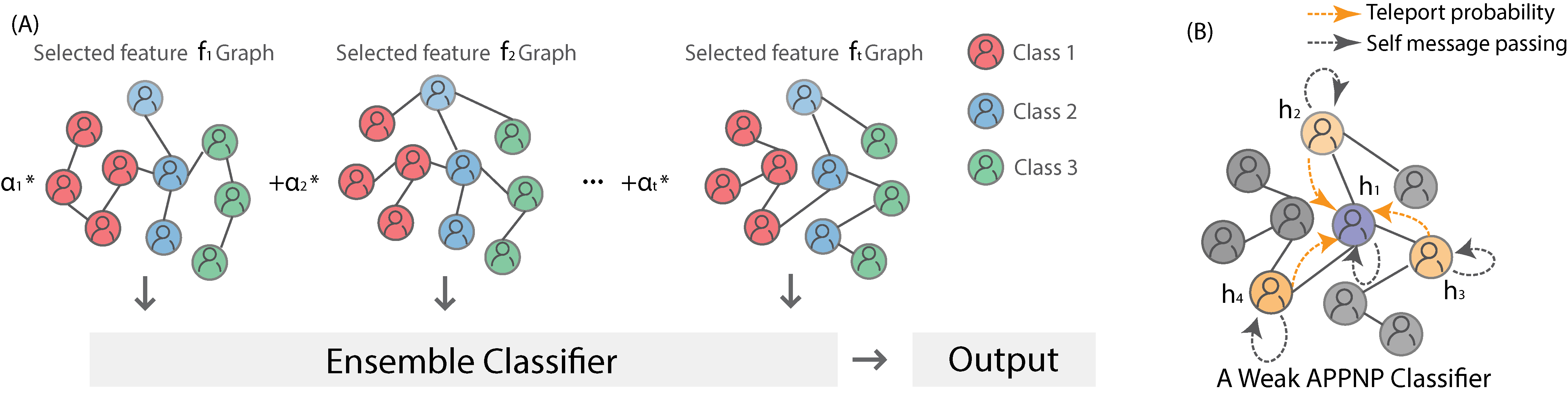
Figure 1: Overview of AdaMedGraph: (A) we iteratively select $T$ features to train $T$ weak classifiers (i.e., APPNP models), and combine them as an ensemble classifier to provide the final prediction. (B) Illustration of features propagation within APPNP weak classifier.

2 Related Work

General tabular data processing methods have been widely used to solve medical-related tasks. While these methods based on feature interactions, such as LR and Wide & Deep, as well as gradient boosting techniques like Gradient Boosting Decision Tree (GBDT) and XGBoost, have shown promise in handling tabular medical data, they tend to focus on feature interactions and often overlook the significance of relationships between patients.

Comparing with general tabular data processing methods, GNNs have the capability to generate embeddings for individual instances by leveraging their inherent information and iteratively gathering messages from neighboring nodes (Gilmer et al., 2017). Well-established GNN methods encompass GCN (Kipf and Welling, 2016), GraphSAGE (Hamilton et al., 2017), graph attention networks (GAT) (Velickovic et al., 2017), and graph isomorphism networks (GIN) (Xu et al., 2018). While GNNs excel at capturing intricate node relationships, they are applicable exclusively when dealing with data structured in a graph format. And the quality of the underlying graph structures significantly influences GNN performance (Zhu et al., 2021). Given that medical tabular data lacks graph structures, the construction of meaningful graphs as inputs for GNNs becomes a critical consideration in this context.

Graph construction for tabular data typically falls into four categories: rule-based, learning-based, search-based, and knowledge-based (Li et al., 2023). (1) The rule-based approach operates by either leveraging inherent data dependencies among data instances and features, e.g., Cvitkovic (2020); Guo et al. (2021); You et al. (2020); Zhu et al. (2003) , or by relying on manually specified heuristics, e.g., Goodge et al. (2022); Rocheteau et al. (2021). The knowledge-based approach uses domain experts to provide insights into the relationships between data instances, enabling fine-grained graph construction (Du et al., 2021). These methods require extra heuristics or knowledge. (2) The learning-based approach for graph construction automatically creates edges between nodes by treating the adjacency matrix as a parameter (Hettige et al., 2020; Liu et al., 2022). However, their internal structures often remain opaque and difficult to understand (Xia et al., 2021). (3) The search-based approach often involves neural architecture search to discover improved graph topologies for representation learning, as demonstrated in (Xie et al., 2021). However, it prioritizes modeling interactions between features rather than samples or patients. Another search-based approach (Du et al., 2022) models data as a bipartite graph, where features with a specific value are regarded as nodes. Such a graph construction method generally excludes numerical variables from the model. Comparing with the current methods, our AdaMedGraph models interactions between patients without the above constraints, provides meaningful automatic graphs constructions, offers an advantage in interpretability, and improves prediction performances.

3 Methods

Given $N$ patients, we have the input $X\in\mathbb{R}^{N*M}$ as patient features, and $Y\in\mathbb{R}^{N*K}$ as the one-hot encoding labels. $M$ is the number of features extracted from multi-model data, and $K$ is the number of label classes. We propose AdaMedGraph to identify different relationships among patients automatically and then classify the patients accurately. The whole process is similar to AdaBoost, with GNNs as weak classifiers. In iteration $t$, to specify each weak classifier $g_{\theta_{t}}$, we need to first select a certain feature $f_{t}$ to measure the similarity of patients to build an adjacency matrix $A_{t}$, and then decide the parameters ${\theta_{t}}$ and $\alpha_{t}$ by training $g_{\theta_{t}}(X,A_{t})$. The overall objective is to minimize the exponential loss $L(g_{T}(X),Y)$ where

$$g_{T}(X)=\sum_{t=1}^{T}\alpha_{t}*g_{\theta_{t}}(X,A_{t}),$$

by finding the optimal $\{f_{t}\}_{t=1,...,T}$, and $\{\theta_{t}\}_{t=1,...,T}$. $\{\alpha_{t}\}_{t=1,...,T}$ denote the weights to ensemble GNNs. fig:Figure1a presents the overview of AdaMedGraph, and we will dive into the details in the following.

Initialization

We first standardize the format of features extracted from multi-modal data by converting them into categorical or numerical values. For example, the images (e.g., MRI) are pre-processed into different brain segments to calculate the volume of grey matter, which serves as an indicator of human cognitive abilities. Additionally, leveraging prior knowledge, genetic data is filtered to retain only the crucial genes associated with the predictions.

At the beginning of the algorithm, we assign the weight of each patient as $w_{i0}=\frac{1}{N}$ where $N$ is the total number of patients. We also specify the type of weak classifiers as Approximate Personalized Propagation of Neural Predictions (APPNP) (Klicpera et al., 2019), a simple yet effective GNN model tailored for graph-structured data.

Constructing the potential $A_{t}$

At iteration $t$, we have the adaptive weights $w_{i,t}$ for data of patient $i$, and the goal is to train a weak classifier $g_{\theta_{t}}$ and the corresponding weight $\alpha_{t}$ of $g_{\theta_{t}}$ to minimize the current weighted loss.

To construct potential adjacency matrices, two things need to be determined: (1) the feature $f_{j,t}$, $j\in[1,M]$ that characterizes a specific relationship among patients, and (2) the threshold $\gamma_{t}$ that determines the existence of edges in $A_{t}$. Specifically, we explore all the features and consider the 16-quantile, 8-quantile, and 4-quantile of the selected feature values as $\gamma_{t}$. The edge between patient $i_{1}$ and $i_{2}$ is equal to $1$ if the absolute difference between their feature values, $|f_{t}(i_{1})-f_{t}(i_{2})|$, is less than or equal to $\gamma_{t}$; otherwise, it is set to $0$. In total, we obtain a set of $\{A_{t}\}$ having $3M$ elements.

Training the weak classifier $g_{\theta_{t}}$

Next, we aim to find an optimal choice of $A_{t}$, $\theta_{t}$ and $\alpha_{t}$ satisfying

$$\min_{A_{t},\theta_{t},\alpha_{t}}L(g_{\theta_{t}}(X,A_{t}),Y)=\sum_{i=1}^{N}w_{i,t}\cdot\exp(-\alpha_{t}\cdot y_{i}\cdot g_{\theta_{t}}(x_{i},A_{t})).$$

Following the SAMME (Zhu et al., 2006), the optimal $\theta_{t}$ is equal to minimize the error at iteration $t$

$$\small\text{err}_{t}=\sum_{i=1}^{N}w_{i,t}\cdot\mathds{1}(y_{i}\neq g_{\theta_{t}}(x_{i},A_{t})),$$

and the corresponding weight $\alpha_{t}$ is calculated by

$$\small\alpha_{t}=\frac{1}{2}\log\frac{1-\text{err}_{t}}{\text{err}_{t}}+\log(K-1).$$

For every $A_{t}$, we can train an APPNP model to obtain $\theta_{t}$ and $\alpha_{t}$. Thus, we explore each possible value in the previous constructed $\{A_{t}\}$ to find a minimal $L(g_{\theta_{t}}(X,A_{t}),Y)$.

After determining the optimal solution, the weights of the patients are updated by

$$w_{i,t+1}=w_{i,t}\cdot\exp(\alpha_{t}\cdot\mathds{1}(y_{i}\neq g_{\theta_{t}}(x_{i},A_{t})),$$

and we proceed to the next iteration.

Termination

The whole process is ended at the iteration $T$ when the error rate of $g_{T}(X)$ or $g_{\theta_{T}}(X,A_{T})$ gets equal or larger than $\frac{K-1}{K}$.

Table 1: PPMI and PDBP 24-month prediction AUROC score. M* is MDS-UPDRS.

	MLP		LR		SVM		RF		XGB		AdaMedGraph
Label	PPMI	PDBP	PPMI	PDBP	PPMI	PDBP	PPMI	PDBP	PPMI	PDBP	PPMI	PDBP
HY	0.593	0.450	0.652	0.504	0.705	0.614	0.664	0.692	0.717	0.643	0.775	0.701
M* I	0.445	0.473	0.601	0.541	0.573	0.554	0.605	0.581	0.625	0.584	0.656	0.586
M* II	0.441	0.499	0.578	0.536	0.570	0.610	0.602	0.598	0.620	0.602	0.651	0.621
M* III	0.695	0.645	0.691	0.648	0.695	0.645	0.670	0.643	0.710	0.610	0.717	0.660
M* Total	0.615	0.577	0.635	0.587	0.634	0.598	0.595	0.579	0.613	0.590	0.646	0.601
M* Axial	0.618	0.552	0.637	0.653	0.661	0.652	0.645	0.657	0.627	0.618	0.661	0.660
M* Rigid	0.644	0.659	0.665	0.656	0.654	0.678	0.663	0.658	0.591	0.626	0.694	0.683
M* Tremor	0.669	0.651	0.689	0.635	0.684	0.619	0.713	0.625	0.672	0.613	0.715	0.685
MoCA	0.519	0.497	0.600	0.694	0.574	0.559	0.573	0.623	0.614	0.684	0.660	0.506
ESS	0.573	0.546	0.573	0.630	0.601	0.628	0.625	0.625	0.611	0.628	0.645	0.631

4 Data and Experiments

In this section, we first introduce prediction tasks and settings in two real-world medical scenarios and then present the results of these tasks.

4.1 PD progression

The longitudinal data from the Parkinson’s Progression Markers Initiative (PPMI) (Marek et al., 2018) and the Parkinson’s Disease Biomarkers Program (PDBP) (Gwinn et al., 2017)are used in our work.

Prediction tasks

We select 10 assessment scores as labels for disease progression: Movement Disorder Society-sponsored Revision of the Unified Parkinson’s Disease Rating Scale (MDS-UPDRS) I, II, III, and total (sum of I, II, and III), and the sub-scores for tremors, axial symptoms, and rigidity in MDS-UPDRS III; Hoehn and Yahr Scale (HY); Montreal Cognitive Assessment (MoCA) total; and Epworth Sleepiness Scale (ESS) total. To get the classification labels, we compute the mean and standard deviation of changes in each score (except HY since HY has a standard classification scale) from baseline to 24-months in the healthy control (HC) group and compare them with the changes in the PD group. By constructing a reference interval based on the HC changes, we then categorize the PD changes as “No Change” if within the interval, or as “Better” or “Worse” if less or more than the interval, respectively.

Feature extraction

We pre-possess genetic data and magnetic resonance imaging (MRI) before training. For MRI, the participant’s T1 scan has been processed into 138 segments, and the volumes of the segments are used as input. For genetic data, the monogenic mutation statuses of GBA, LRRK2, SNCA, and APOE_E4 are encoded as binary variables.

Dataset statistics and division

Two sets of experiments have been designed for the PD progression task. In PD Experiment I, we utilize clinical assessments and genetic data as input features, comprising a total of 78 variables, given the absence of MRI data in the PDBP dataset. The PPMI dataset is split into a training set (80%, n = 358) and an internal testing set (20%, n = 90). Besides, we randomly select 20% of the training data as our validation set during training to select the final best models. The PDBP dataset serves as an external validation dataset (n = 228).

In Experiment II, we expand the range of input features to include clinical assessments, MRI data, and genetic information, resulting in a total of 234 variables. This study exclusively utilizes the PPMI dataset, which has been divided into an 80% training set (n = 252) and a 20% testing set (n = 65). Similarly, 20% of training data has been randomly separated as validation set. In both experiments, the train-test split is based on participants’ enrollment times, with the earlier visit participants assigned to the training set while the later visit participants are allocated to the testing set, while the validation split is done randomly.

Baselines

To evaluate the performance of our model, we include several ML classification methods as baseline models. The aforementioned models have frequently been employed in medical classification tasks, encompassing a 2-layer Multilayer Perceptron (MLP), a logistic regression classifier (LR), a random forest classifier (RF), a support vector machine classifier (SVM), and a XGBoost model. Furthermore, in order to comprehend the importance of automatically selecting edge features, we construct a graph based on prior knowledge. Since it is well-known that age is a critical factor for PD progression, we construct a graph based on age (with a threshold of 5) and develop an APPNP (referred to as APPNP-Age) as a comparative model in experiment II.

4.2 Metabolic syndrome

In the metabolic syndrome prediction task, we include 109,027 individuals in the UK Biobank (Sudlow et al., 2015) (80% for training and 20% for testing). All subjects have no record of metabolic syndrome on their baseline screen, and their 168 proton nuclear magnetic resonance (NMR) metabolic biomarkers and 17 traditional clinical risk variables are used as input (Lian and Vardhanabhuti, 2023) to predict whether participants will have the diseases after a period of time. The input data has been processed into 9 principal components using principal component analysis, and XGBoost and TabNet (Arik and Pfister, 2021) are implemented as baseline models.

4.3 Results

We utilize the weighted area under the receiver operating characteristic curve (AUROC) as the evaluation metric for all tasks.

PD progression

In the context of predicting 24-month progression experiment I, our AdaMedGraph model has received greater accuracy in comparison to all baseline models across all labels, with the exception of MoCA in the PDBP dataset. This discrepancy can be attributed to differences in the distribution of selected edge features for MoCA between the two datasets. These superior results from our model underscore the significance of incorporating both intra- and inter-patient data for individual disease progression prediction. Refer to the tab:PPMIPDBP for a comprehensive understanding of the performances.

In experiment II, AdaMedGraph also exhibits superior performance when compared to all the baseline models as well as APPNP-age, which suggests that taking into account automatically selected relationships among patients can significantly enhance the performance of prediction. Please refer to tab:PPMI for details.

Table 2: PPMI 24-month prediction AUROC score. A-A is APPNP-Age. M* is MDS-UPDRS.

Label	MLP	LR	SVM	RF	XGB	A-A	Ours
HY	0.556	0.630	0.594	0.633	0.643	0.630	0.682
M* I	0.543	0.638	0.531	0.593	0.628	0.699	0.730
M* II	0.507	0.588	0.573	0.457	0.575	0.621	0.652
M* III	0.409	0.583	0.587	0.553	0.566	0.604	0.666
M* Total	0.648	0.617	0.593	0.590	0.598	0.563	0.684
M* Axial	0.517	0.610	0.610	0.549	0.538	0.591	0.689
M* Rigid	0.419	0.572	0.636	0.548	0.628	0.682	0.693
M* Tremor	0.520	0.628	0.648	0.657	0.700	0.585	0.700
MoCA	0.680	0.713	0.672	0.714	0.723	0.668	0.746
ESS	0.537	0.623	0.639	0.645	0.596	0.649	0.676

Metabolic syndrome

In the context of predicting the occurrence of metabolic syndrome, the AdaMedGraph model demonstrates superior performance with an area under the AUROC of 0.675 on the testing dataset. This surpasses both the XGBoost model, which achieved an AUROC of 0.641, and the TabNet model, which achieved an AUROC of 0.672.

5 Discussion

In this study, we introduce an innovative algorithm, namely AdaMedGraph, designed to autonomously identify important features for the construction of multiple patient similarity graphs, which serve as the basis for training GNNs in an AdaBoost framework, thereby enhancing the accuracy of classification tasks. We have conducted two sets of clinical experiments, and the results affirm our initial hypothesis that automatically constructing multi-relationship graphs among patients using inter- and intra-individual data can benefit personalized medicine.

One thing that needs to be noticed is the computational cost of our AdaMedGraph. Although our model goes through all potential features to construct a total of $3M$ graphs during training, it’s important to note that we use the APPNP model as the weak classifier, known for its relatively low computational cost, with only linear computational complexity. In this case, the total computational cost of our model is acceptable. In our experiments, we have observed reasonable training time costs. For instance, in our PD prediction task with 234 input features and 317 patient samples, the training process has taken less than 5 minutes. Similarly, for the metabolic syndrome prediction task, which includes 109,027 patients and 9 features, it takes less than 30 minutes for training. These experiments have been conducted on a single V100 GPU. Furthermore, to optimize for high-dimensional settings, a simple feature selection process could be integrated before searching for the best features.

Appendix A Ethics Statement

The population cohort in the metabolic syndrome experiments is from the UK Biobank [Application Number 78730] which has received ethical approval from the North West Multicentre Research Ethics Committee (REC reference: 11/NW/03820). All participants have given written informed consent before enrolment.

PD study data is retrieved from AMPPD platform https://amp-pd.org/ using the terms of the AMP-PD Data Use Agreement and PPMI website https://www.ppmi-info.org/. The data has used in this study has been collected before the commencement of our study and has been obtained in an anonymized format. In the original PPMI and PDBP studies, participants have previously consented in writing to the sharing of their data. These investigations have been conducted in accordance with protocols authorized by the Indiana University Institutional Review Board (IRB) for PPMI and the respective PDBP centers.

Appendix B Hyper-parameters

We list the hyper-parameters of baseline models and AdaMedGraph in this part. Grid search method has used for all models.

B.1 Task 1

MLP

We train the MLP models with Adam optimizer and search the hyper-parameters of hidden dimension in {128, 256, 512, 1024}, L2 regularization in {$10^{-5}$, $10^{-4}$, $10^{-3}$}, learning rate {$10^{-5}$, $5*10^{-4}$, $10^{-4}$, $5*10^{-3}$}, dropout in {0.1, 0.3, 0.5} and total epoch in {100, 200, 300}.

LR

We search the LR models hyper-parameters of regularization method in {L1, L2, elastic net} and strength of the regularization in {0.01, 0.1, 1, 10}.

SVM

We search the the LR models hyper-parameters of kernels in {linear, polynomial, radial basis function} and strength of the regularization in in {0.01, 0.1, 1, 10}.

RF

We search the LR models hyper-parameters of number of estimators in {50, 100, 150, 200 }, max depth in {10, 20, 30, 40, 50}, minimum number of samples required to be at a leaf node in {1, 2, 4}, and the minimum number of samples required to split an internal node in {1, 2, 3}.

XGB

We list the XGB models hyper-parameters searching in tab:xgbtable.

Table 3: XGBoost hyper-parameters search list

Hyper-parameter	Tunning Range
Number of estimators	{50, 75, 100, 150, 200}
Max depth	{1, 2, 3, 6, 9}
Learning rate	{0.001, 0.01, 0.1, 0.3, 0.5}
Min child weight	{1, 2, 3, 4, 5}
Gamma	{ 0.5, 1, 2, 3, 6, 9}
Colsample by tree	{0, 0.25, 0.5, 0.75, 1}
Colsample by level	{0, 0.25, 0.5, 0.75, 1}
lambda	{0.05, 0.1, 0.25, 0.5, 1}
alpha	{0.5, 1, 10}

APPNP-Age

We train our APPNP-Age with Adam optimizer, Cosine Annealing Scheduler for weight decay, and 100 total epochs. We search the hyper-parameters of hidden dimension of linear layer (H) in {128, 256, 512}, number of iterations (k) in {3, 5, 10}, teleport probability in {0.1, 0.3, 0.5, 1}, dropout in {0.1, 0.3, 0.5}, learning rate in {$10^{-5}$, $5*10^{-4}$, $10^{-4}$, $5*10^{-3}$ }, and threshold for age in {4, 4.5, 5, 5.5, 6}.

AdaMedGraph

The training details for AdaMedGraph contain two parts: training a single APPNP and training AdaBosst. The details have been summarized in tab:adamed.

Table 4: AdaMedGraph hyper-parameter list. Hyper-parameters in braces are searched.

Single APPNP
Optimizer	Adam
Weight decay	{0.00001, 0.0001, 0.001}
Learning rate decay	Cosine Annealing Scheduler
Learning rate	{$10^{-5}$, $5*10^{-5}$, $10^{-4}$, $5*10^{-4}$, $10^{-3}$, $5*10^{-3}$}
Total epoch	{100, 150, 200}
Early stop	{5, 10, 20}
H	{128, 256, 512}
k	{3, 5, 10}
Teleport probability	{0.1, 0.3, 0.5, 1}
Dropout	{0.1, 0,3, 0,5}
AdaBoost
Number of estimators	{5, 10, 15, 20}
Learning rate	{0.1, 0.33, 0.5, 0.66, 1}

B.2 Task 2: metabolic syndrome prediction

XGB

We list the XGB models hyper-parameters searching in tab:xgbtable2.

Table 5: XGBoost hyper-parameters search list for metabolic syndrome prediction

Hyper-parameter	Tunning Range
Number of estimators	{50, 100, 200, 300}
Max depth	{3, 6, 9, 12}
Learning rate	{0.001, 0.01, 0.1, 0.3, 0.5}
Min child weight	{1, 2, 3, 4, 5}
Gamma	{ 0.5, 1, 3, 6, 9, 12}
Colsample by tree	{0, 0.5, 1}
Colsample by level	{0, 0.5, 1}
lambda	{0.05, 0.1, 0.25, 0.5, 1}
alpha	{0.001, 0.01, 0.5, 1, 10}

TabNet

We Search the TabNet models hyper-parameters of mask type in {”entmax”, ”sparsemax”}, the width of the decision prediction layer and the attention embedding for each mask in {32, 48, 56, 64}, number of steps in {1, 2, 3}, gamma in {1.0, 1.2, 1.4}, the number of shared Gated Linear Units at each step in {1, 2, 3}, learning rate in {$10^{-5}$, $5*10^{-5}$, $10^{-4}$, $5*10^{-4}$, $10^{-3}$, $5*10^{-3}$} and lambda space in {$10^{-5}$, $10^{-4}$}.

AdaMedGraph

The training details for AdaMedGraph on task 2 have been summarized in tab:adamed2.

Table 6: AdaMedGraph hyper-parameter for metabolic syndrome prediction. Hyper-parameters in braces are searched.

Single APPNP
Optimizer	Adam
Weight decay	{0.00001, 0.0001, 0.001}
Learning rate decay	Cosine Annealing Scheduler
Learning rate	{$10^{-5}$, $5*10^{-5}$, $10^{-4}$, $5*10^{-4}$, $10^{-3}$, $5*10^{-3}$}
Total epoch	{100, 200, 500, 1000}
Early stop	{10, 20, 30}
H	{128, 256, 512}
k	{3, 5, 10}
Teleport probability	{0.1, 0.3, 0.5, 1}
Dropout	{0.1, 0,3, 0,5}
AdaBoost
Number of estimators	{5, 10, 15, 20}
Learning rate	{0.1, 0.33, 0.5, 0.66, 1}

References

- Arik and Pfister (2021) Sercan Ö Arik and Tomas Pfister. Tabnet: Attentive interpretable tabular learning. In Proceedings of the AAAI conference on artificial intelligence, volume 35, pages 6679–6687, 2021.
- Cvitkovic (2020) Milan Cvitkovic. Supervised learning on relational databases with graph neural networks. International Conference on Learning Representations, 2020.
- Du et al. (2022) Kounianhua Du, Weinan Zhang, Ruiwen Zhou, Yangkun Wang, Xilong Zhao, Jiarui Jin, Quan Gan, Zheng Zhang, and David P Wipf. Learning enhanced representation for tabular data via neighborhood propagation. Advances in Neural Information Processing Systems, 35:16373–16384, 2022.
- Du et al. (2021) Lun Du, Fei Gao, Xu Chen, Ran Jia, Junshan Wang, Jiang Zhang, Shi Han, and Dongmei Zhang. Tabularnet: A neural network architecture for understanding semantic structures of tabular data. In Proceedings of the 27th ACM SIGKDD Conference on Knowledge Discovery & Data Mining, pages 322–331, 2021.
- Gilmer et al. (2017) Justin Gilmer, Samuel S Schoenholz, Patrick F Riley, Oriol Vinyals, and George E Dahl. Neural message passing for quantum chemistry. In International conference on machine learning, pages 1263–1272. PMLR, 2017.
- Goodge et al. (2022) Adam Goodge, Bryan Hooi, See-Kiong Ng, and Wee Siong Ng. Lunar: Unifying local outlier detection methods via graph neural networks. In Proceedings of the AAAI Conference on Artificial Intelligence, volume 36, pages 6737–6745, 2022.
- Guo et al. (2021) Xiawei Guo, Yuhan Quan, Huan Zhao, Quanming Yao, Yong Li, and Weiwei Tu. Tabgnn: Multiplex graph neural network for tabular data prediction. The 3rd Workshop on Deep Learning Practice for High-Dimensional Sparse Data with KDD (DLP-KDD), 2021.
- Gwinn et al. (2017) Katrina Gwinn, Karen K David, Christine Swanson-Fischer, Roger Albin, Coryse St Hillaire-Clarke, Beth-Anne Sieber, Codrin Lungu, F DuBois Bowman, Roy N Alcalay, Debra Babcock, et al. Parkinson’s disease biomarkers: perspective from the NINDS Parkinson’s disease biomarkers program. Biomarkers in medicine, 11(6):451–473, 2017.
- Hamilton et al. (2017) Will Hamilton, Zhitao Ying, and Jure Leskovec. Inductive representation learning on large graphs. Advances in neural information processing systems, 30, 2017.
- Hettige et al. (2020) Bhagya Hettige, Weiqing Wang, Yuan-Fang Li, Suong Le, and Wray Buntine. Medgraph: Structural and temporal representation learning of electronic medical records. In ECAI 2020, pages 1810–1817. IOS Press, 2020.
- Hulsen et al. (2019) Tim Hulsen, Saumya S Jamuar, Alan R Moody, Jason H Karnes, Orsolya Varga, Stine Hedensted, Roberto Spreafico, David A Hafler, and Eoin F McKinney. From big data to precision medicine. Frontiers in medicine, 6:34, 2019.
- Kipf and Welling (2016) Thomas N Kipf and Max Welling. Semi-supervised classification with graph convolutional networks. In International Conference on Learning Representations, 2016.
- Klicpera et al. (2019) Johannes Klicpera, Aleksandar Bojchevski, and Stephan Günnemann. Predict then propagate: Graph neural networks meet personalized pagerank. 2019.
- Li et al. (2023) Cheng-Te Li, Yu-Che Tsai, and Jay Chiehen Liao. Graph neural networks for tabular data learning. In 2023 IEEE 39th International Conference on Data Engineering (ICDE), pages 3589–3592. IEEE, 2023.
- Lian and Vardhanabhuti (2023) Jie Lian and Varut Vardhanabhuti. Metabolic biomarkers using nuclear magnetic resonance metabolomics assay for the prediction of aging-related disease risk and mortality: a prospective, longitudinal, observational, cohort study based on the uk biobank. GeroScience, pages 1–12, 2023.
- Liu et al. (2022) Yixin Liu, Yu Zheng, Daokun Zhang, Hongxu Chen, Hao Peng, and Shirui Pan. Towards unsupervised deep graph structure learning. In Proceedings of the ACM Web Conference 2022, pages 1392–1403, 2022.
- Marek et al. (2018) Kenneth Marek, Sohini Chowdhury, Andrew Siderowf, Shirley Lasch, Christopher S Coffey, Chelsea Caspell-Garcia, Tanya Simuni, Danna Jennings, Caroline M Tanner, John Q Trojanowski, et al. The Parkinson’s progression markers initiative (PPMI)–establishing a PD biomarker cohort. Annals of clinical and translational neurology, 5(12):1460–1477, 2018.
- Mhasawade et al. (2021) Vishwali Mhasawade, Yuan Zhao, and Rumi Chunara. Machine learning and algorithmic fairness in public and population health. Nature Machine Intelligence, 3(8):659–666, 2021.
- Parisot et al. (2017) Sarah Parisot, Sofia Ira Ktena, Enzo Ferrante, Matthew Lee, Ricardo Guerrerro Moreno, Ben Glocker, and Daniel Rueckert. Spectral graph convolutions for population-based disease prediction. In Medical Image Computing and Computer Assisted Intervention- MICCAI 2017: 20th International Conference, Quebec City, QC, Canada, September 11-13, 2017, Proceedings, Part III 20, pages 177–185. Springer, 2017.
- Rocheteau et al. (2021) Emma Rocheteau, Catherine Tong, Petar Veličković, Nicholas Lane, and Pietro Liò. Predicting patient outcomes with graph representation learning. International Workshop on Deep Learning on Graphs: Method and Applications (DLG-AAAI), 2021.
- Shilo et al. (2020) Smadar Shilo, Hagai Rossman, and Eran Segal. Axes of a revolution: challenges and promises of big data in healthcare. Nature medicine, 26(1):29–38, 2020.
- Sudlow et al. (2015) Cathie Sudlow, John Gallacher, Naomi Allen, Valerie Beral, Paul Burton, John Danesh, Paul Downey, Paul Elliott, Jane Green, Martin Landray, et al. Uk biobank: an open access resource for identifying the causes of a wide range of complex diseases of middle and old age. PLoS medicine, 12(3):e1001779, 2015.
- Tu et al. (2023) Tao Tu, Shekoofeh Azizi, Danny Driess, Mike Schaekermann, Mohamed Amin, Pi-Chuan Chang, Andrew Carroll, Chuck Lau, Ryutaro Tanno, Ira Ktena, et al. Towards generalist biomedical AI. arXiv preprint arXiv:2307.14334, 2023.
- Velickovic et al. (2017) Petar Velickovic, Guillem Cucurull, Arantxa Casanova, Adriana Romero, Pietro Lio, Yoshua Bengio, et al. Graph attention networks. stat, 1050(20):10–48550, 2017.
- Xia et al. (2021) Feng Xia, Ke Sun, Shuo Yu, Abdul Aziz, Liangtian Wan, Shirui Pan, and Huan Liu. Graph learning: A survey. IEEE Transactions on Artificial Intelligence, 2(2):109–127, 2021.
- Xie et al. (2021) Yuexiang Xie, Zhen Wang, Yaliang Li, Bolin Ding, Nezihe Merve Gürel, Ce Zhang, Minlie Huang, Wei Lin, and Jingren Zhou. Fives: Feature interaction via edge search for large-scale tabular data. In Proceedings of the 27th ACM SIGKDD Conference on Knowledge Discovery & Data Mining, pages 3795–3805, 2021.
- Xing et al. (2019) Xiaodan Xing, Qingfeng Li, Hao Wei, Minqing Zhang, Yiqiang Zhan, Xiang Sean Zhou, Zhong Xue, and Feng Shi. Dynamic spectral graph convolution networks with assistant task training for early MCI diagnosis. In International Conference on Medical Image Computing and Computer-Assisted Intervention, pages 639–646. Springer, 2019.
- Xu et al. (2018) Keyulu Xu, Weihua Hu, Jure Leskovec, and Stefanie Jegelka. How powerful are graph neural networks? In International Conference on Learning Representations, 2018.
- You et al. (2020) Jiaxuan You, Xiaobai Ma, Yi Ding, Mykel J Kochenderfer, and Jure Leskovec. Handling missing data with graph representation learning. Advances in Neural Information Processing Systems, 33:19075–19087, 2020.
- Zhang et al. (2023) Kai Zhang, Jun Yu, Zhiling Yan, Yixin Liu, Eashan Adhikarla, Sunyang Fu, Xun Chen, Chen Chen, Yuyin Zhou, Xiang Li, et al. BiomedGPT: A unified and generalist biomedical generative pre-trained transformer for vision, language, and multimodal tasks. arXiv preprint arXiv:2305.17100, 2023.
- Zheng et al. (2022) Shuai Zheng, Zhenfeng Zhu, Zhizhe Liu, Zhenyu Guo, Yang Liu, Yuchen Yang, and Yao Zhao. Multi-modal graph learning for disease prediction. IEEE Transactions on Medical Imaging, 41(9):2207–2216, 2022.
- Zhu et al. (2006) Ji Zhu, Saharon Rosset, Hui Zou, and Trevor Hastie. Multi-class adaboost. Ann Arbor, 1001:48109, 2006.
- Zhu et al. (2003) Xiaojin Zhu, Zoubin Ghahramani, and John D Lafferty. Semi-supervised learning using gaussian fields and harmonic functions. In Proceedings of the 20th International conference on Machine learning (ICML-03), pages 912–919, 2003.
- Zhu et al. (2021) Yanqiao Zhu, Weizhi Xu, Jinghao Zhang, Qiang Liu, Shu Wu, and Liang Wang. Deep graph structure learning for robust representations: A survey. CoRR, abs/2103.03036, 2021. URL https://arxiv.org/abs/2103.03036.