Soft limit of higher-spin interactions in the IKKT model

Abstract

We study interactions of the higher-spin gauge theory arising from the IKKT matrix model on covariant FLRW quantum space-time, denoted as HS-IKKT. We elaborate some vertices explicitly, which are not manifestly Lorentz invariant in the unitary formulation. The vertices are exponentially suppressed in the asymptotically flat and late-time regime, for energies below the scale of non-commutativity. We work out some vertices and amplitudes for low external spin, and show how Weinberg’s soft theorem is avoided. Moreover, we show that Lorentz invariance can be recovered at least for some vertices in the covariant formulation, at the expense of locality. The lowest-spin sector of this theory is expected to be governed by an “almost”-Lorentz-invariant Yang-Mills gauge theory coupled to emergent gravity.

1 Introduction

The idea that gravity can emerge from suitable non-gravitational or “pre-gravity” models dates back to the late 60’s [1, 2]. Such a mechanism was recently exhibited in the IKKT matrix model [3], which can be viewed as a constructive description of type IIB superstring theory. In particular, it was shown that a version of modified GR can arise from quantum effects of the IKKT matrix model on a suitable type of background [5, 6]. The mechanism requires 3+1 dimensional quantized spacetime branes without compactification of target space, and thereby avoids the problem of vacuum selection in the string landscape. For related progress on the non-perturbative selection of spacetime using a numerical approach see e.g. [7, 8] and references therein.

To avoid (or reduce) explicit breaking of Lorentz invariance in this setting, we consider the IKKT matrix model on a suitable type of background brane $\mathcal{M}\xhookrightarrow{}\mathbb{R}^{1,9}$ with the structure of covariant quantum space, such as fuzzy $S_{N}^{4}$ or $H_{N}^{4}$. On such a background, the matrix model induces a higher-spin gauge theory in terms of higher-spin valued fluctuations, see e.g. [9, 10]. Unlike the standard higher-spin gravity (HSGRA) in $d\geq 4$ [11, 12] with a spectrum of infinitely many fields with spin $s=0,1,\ldots,\infty$, the higher-spin gauge theory induced by the IKKT matrix model (HS-IKKT) typically leads to a truncated tower of higher-spin modes in 4 dimensions. Moreover, the number of physical degrees of freedom for a Lorentzian real gauge field with internal spin-$s$ in HS-IKKT theory is $2(2s+1)$. This makes Lorentzian HS-IKKT theory a would-be massive theory with mass scale set by the cosmic curvature. Nevertheless, since HS-IKKT is free of ghosts (negative norm states) [15] and can be defined on a cosmological spacetime with Lorentzian signature, we can use standard QFT techniques to study the corresponding theory.

Given all the above features of HS-IKKT, the following question naturally arises: How can HS-IKKT surpass all the obstructions posed by no-go theorems [16, 17]? This is the question we want to address in the present paper.

Since Lorentzian HS-IKKT is not massless in the strict sense, one might argue that the standard implications of no-go theorems simply do not apply to this theory. However, it is still a gauge theory which is “almost” massless, and a detailed study of the standard arguments leading to soft theorems or factors resulting from gauge invariance of the $S$-matrix is required to address this question. In this work, we elaborate some vertices of the Lorentzian theory explicitly and study their physical significance.

Our first main result is that gauge invariance of the $S$-matrix in the soft limit is trivially satisfied in Lorentzian HS-IKKT theory for the cubic vertices, without implying any soft theorems. Namely, there are no non-trivial constraints in terms of external momentum in the soft limit. Although this may seem counter-intuitive, it is a direct consequence of the manifest gauge invariance of the model.

Furthermore, we observe that the cubic vertices for the lowest spin components of the fields vanish. This means that the standard cubic sector of the theory is non-interacting. Nevertheless, the theory is not free: non-trivial cubic vertices involving higher-spin modes do arise, which are suppressed in the late-time, almost-flat regime of the theory. Moreover, the quartic vertices of the theory are non-trivial even with the lowest spin components of fields. These vertices are “mildly Lorentz-violating”, i.e. they involve the explicit time-like vector field defined by the FLRW background geometry. More explicitly, all cubic vertices are suppressed by a factor of $L^{2}_{\rm NC}\,e^{-\frac{3\tau}{2}}$ in the late time regime, while quartic vertices are suppressed by a factor of $L^{4}_{\rm NC}\,e^{-3\tau}$. Here $\tau$ parametrizes the cosmic time of the FLRW background, and $L_{\rm NC}$ is a non-commutative length scale. This means that classically, the Lorentzian HS-IKKT theory is almost-free. To confirm this result, we compute some 3-amplitudes of HS-IKKT with the obtained vertices explicitly. We also spell out the fusion rules, and study the simplest 4-point tree-level amplitude.

Finally, we observe that at least some of these apparently Lorentz-violating interactions can in fact be rewritten in a manifestly covariant form, where Lorentz invariance is effectively recovered due to gauge invariance. This suggests that Lorentz invariance should be understood here in a somewhat non-standard way as part of the gauge symmetry.

This paper is organized as follows. Section 2 provides a brief review of the (HS-)IKKT matrix model on a fuzzy $SO(1,3)$-invariant spacetime called $\mathcal{M}^{1,3}$. Section 3 derives some cubic and quartic vertices between (higher-spin) fields of the model. The soft limit of higher-spin scatterings associated with the cubic vertices is also discussed. Some 3-point amplitudes are computed explicitly, and the simplest 4-point amplitude is also studied. Finally, Section 4 summarizes the results and discusses future direction.

2 Review of the higher-spin IKKT model

We consider the semi-classical form of the $SO(1,9)$-invariant IKKT matrix model in the large $N$ limit, given by the action

$$S=\int\,\Big{(}\{t^{\boldsymbol{I}},t^{\boldsymbol{J}}\}\{t_{\boldsymbol{I}},t_{\boldsymbol{J}}\}+2m^{2}t_{\boldsymbol{I}}t^{\boldsymbol{I}}+\ldots\Big{)}\,,\qquad\boldsymbol{I}=0,1,\ldots,9\,.$$ (2.1)

Here $t^{\boldsymbol{I}}:=\langle\zeta|T^{\boldsymbol{I}}|\zeta\rangle$ play the role of embedding functions of some underlying quantized brane in $\mathbb{R}^{1,9}$, defined by the expectation values of $N\times N$ Hermitian background matrices $T^{\boldsymbol{I}}$ w.r.t. suitable localized quasi-coherent states $|\zeta\rangle\in\mathcal{H}$ of some Hilbert space $\mathcal{H}$. The Poisson brackets arise from commutators of the matrix model in the semi-classical regime. In this language, the action is invariant under gauge transformations $t^{\boldsymbol{I}}\to t^{\boldsymbol{I}}+\{t^{\boldsymbol{I}},\Lambda\}$ for $\Lambda$ a gauge parameter. This geometrical approach to the matrix model is reviewed e.g. in [4]. The ellipses in (2.1) stand for the fermionic part, and a mass term $m^{2}$ is added to set the scale for the theory.

For our purpose of studying soft theorems, we will consider the interactions between the higher-spin valued scalar fields transforming under $SO(6)$, and a higher-spin gauge field. It is thus sufficient to consider only the bosonic part of the model.

Field content in $4d$ Lorentzian IKKT.

We will study the (HS-)IKKT theory on an $SO(1,3)$-invariant cosmological spacetime $\mathcal{M}^{1,3}$ in the flat limit. This manifold arises as a 3+1 dimensional degenerate embedding of the non-compact complex projective space $\mathbb{P}^{1,2}$ in the target space. Here $\mathbb{P}^{1,2}$ is viewed as a $S^{2}$ bundle over $\mathcal{M}^{1,3}$ described by Cartesian coordinate functions $y^{\mu}$, while $S^{2}$ is described by $\underline{\mathtt{t}}^{\mu}$ and encodes the higher-spin structure. The explicit relations are reviewed in appendix A. We consider fluctuations around the background $\underline{\mathtt{t}}^{\boldsymbol{I}}$ where

$$t^{\boldsymbol{I}}=\binom{\underline{\mathtt{t}}^{\mu}}{0}+\binom{\mathsf{a}^{\mu}}{\phi^{\boldsymbol{\mathtt{I}}}}\,,\qquad\mu=0,1,2,3\,,\qquad\boldsymbol{\mathtt{I}}=4,\ldots,9\,.$$ (2.2)

Here, $\mathsf{a}^{\mu}$ play the role of (non-commutative, $\mathfrak{hs}$-valued) gauge fields. With this organization, the action (2.1) becomes [10]

$$S=\int \mho\,\Big{(}\frac{1}{2}\{\underline{\mathtt{t}}^{\mu},\mathsf{a}^{\nu}\}\{\underline{\mathtt{t}}_{\mu},\mathsf{a}_{\nu}\}+\{\underline{\mathtt{t}}_{\mu},\underline{\mathtt{t}}_{\nu}\}\{\mathsf{a}^{\mu},\mathsf{a}^{\nu}\}+\frac{1}{2}\{\underline{\mathtt{t}}^{\mu},\mathsf{a}^{\mu}\}^{2}+\frac{1}{2}\{\underline{\mathtt{t}}^{\mu},\phi^{\boldsymbol{\mathtt{I}}}\}\{\underline{\mathtt{t}}_{\mu},\phi_{\boldsymbol{\mathtt{I}}}\}$$

$$+\{\underline{\mathtt{t}}^{\mu},\mathsf{a}^{\nu}\}\{\mathsf{a}_{\mu},\mathsf{a}_{\nu}\}+\{\underline{\mathtt{t}}^{\mu},\phi^{\boldsymbol{\mathtt{I}}}\}\{\mathsf{a}_{\mu},\phi_{\boldsymbol{\mathtt{I}}}\}$$

$$+\frac{1}{4}\{\mathsf{a}^{\mu},\mathsf{a}^{\nu}\}\{\mathsf{a}_{\mu},\mathsf{a}_{\nu}\}+\frac{1}{2}\{\mathsf{a}^{\mu},\phi^{\boldsymbol{\mathtt{I}}}\}\{\mathsf{a}_{\mu},\phi_{\boldsymbol{\mathtt{I}}}\}+\frac{1}{4}\{\phi^{\boldsymbol{\mathtt{I}}},\phi^{\boldsymbol{\mathtt{J}}}\}\{\phi_{\boldsymbol{\mathtt{I}}},\phi_{\boldsymbol{\mathtt{J}}}\}+\ldots\Big{)}+S_{\mathtt{BG}}\ .$$ (2.3)

Here $S_{\mathtt{BG}}$ is the background action, which consists of terms that are zeroth or first order in fields. Moreover,

$$\mho:=\frac{R}{y^{4}}dy^{0}dy^{1}dy^{2}dy^{3}=(\sinh(\tau))^{-1}d^{4}y$$ (2.4)

is the induced measure, and $y^{a}:=\langle\zeta|Y^{a}|\zeta\rangle\in\mathbb{R}^{1,4}$ for $a=0,1,2,3,4$ are coordinates of $H^{4}$. This 4-hyperboloid of radius $R$ is defined by $\eta^{ab}y_{a}y_{b}=-R^{2}$, where $\eta^{ab}=\,\mathrm{diag}(-,+,+,+,+)$. The $SO(1,3)$-invariant space-time $\mathcal{M}^{1,3}$ is then obtained as a projection to $\mathbb{R}^{1,3}$, with the time parameter $\tau$ defined via $y_{4}=R\sinh(\tau)$. On this spacetime $\mathcal{M}^{1,3}$, the Poisson brackets between $\underline{\mathtt{t}}$ and $y$ define a frame

$$E^{\mu\nu}:=\{\underline{\mathtt{t}}^{\mu},y^{\nu}\} =\frac{\eta^{\mu\nu}}{R}y^{4}=\eta^{\mu\nu}\sinh(\tau)\,,\qquad\eta^{\mu\nu}=\,\mathrm{diag}(-,+,+,+)\,,$$ (2.5)

for $\mu,\nu=0,1,2,3$, and the effective metric governing the local physics is found in [18] to be

$$G_{\mu\nu}=\sinh(\tau)\eta_{\mu\nu}\ \propto\ \eta_{\mu\nu}\ .$$ (2.6)

Since we are only interested in the local physics here, we will absorb the conformal factor in the propagating fields under consideration, so that the local effective metric coincides with the Minkowski metric $\eta_{\mu\nu}$ in the Cartesian coordinates $y^{\mu}$. In particular, we have

$$\{\underline{\mathtt{t}}_{\mu},f(y)\}=\sinh(\tau)\partial_{\mu}f(y)\,,\qquad\partial_{\mu}:=\partial/\partial y^{\mu}\,,\qquad\partial_{\mu}y^{\nu}=\delta_{\mu}{}^{\nu}$$ (2.7)

where $\underline{\mathtt{t}}_{\mu}$ defines the ‘momenta’ on $\mathcal{M}^{1,3}$. Further relations between $\underline{\mathtt{t}}$’s and $y$’s are collected in Appendix A.

Higher-spin modes on $\mathcal{M}^{1,3}$.

All higher-spin modes on $\mathcal{M}^{1,3}$ are captured by the following expansion

$$\phi^{\boldsymbol{\mathtt{I}}}(y|\underline{\mathtt{t}})=\sum_{s}\varphi^{\boldsymbol{\mathtt{I}}}{}_{\nu(s)}(y)\,\underline{\mathtt{t}}^{\nu(s)}\,,\qquad\mathsf{a}_{\mu}(y|\underline{\mathtt{t}})=\sum_{s}\mathcal{A}_{\mu|\nu(s)}(y)\,\underline{\mathtt{t}}^{\nu(s)}\,,$$ (2.8)

where $\underline{\mathtt{t}}^{\mu}$ are generators of the space-like internal fuzzy 2-sphere $S_{N}^{2}$ underlying the higher-spin structures of the model, and $\underline{\mathtt{t}}^{\nu(s)}=\underline{\mathtt{t}}^{\nu_{1}}\ldots\underline{\mathtt{t}}^{\nu_{s}}$.

For our purposes of studying soft theorems on flat Lorentzian background, we can decompose $\mathcal{A}_{\mu|\nu(s)}$ as [10]

$$\mathcal{A}_{\mu|\nu(s)}=A_{(\nu(s)\mu)}+\eta_{\mu\nu}\tilde{\mathsf{A}}_{\nu(s-1)}+y_{\mu}\zeta_{\nu(s)}+\partial_{\mu}\tilde{\zeta}_{\nu(s)}\,.$$ (2.9)

Then, upon imposing the gauge fixing condition [19]

$$\mathcal{G}(\mathsf{a})=\{\underline{\mathtt{t}}_{\mu},\mathsf{a}^{\mu}\}=0$$ (2.10)

and quotienting out the linearized gauge transformations $\delta\mathsf{a}^{\mu}=\{\underline{\mathtt{t}}^{\mu},\Lambda\}$, one can check that $\mathcal{A}_{\mu|\nu(s)}$ carry $2(2s+1)$ physical dof.. Likewise, $\varphi^{\boldsymbol{\mathtt{I}}}{}_{\nu(s)}$ carries $6(2s+1)$ dof. Thus, as alluded in the introduction, HS-IKKT is not a conventional higher-spin theory.

After performing the gauge fixing procedure described above, the physical higher-spin gauge fields admit the decomposition

$$\mathsf{a}_{\mu}=\sum_{s}\mathcal{A}_{\mu|\nu(s)}(y)\underline{\mathtt{t}}^{\nu(s)}=\sum_{s}\Big{(}A_{(\nu(s)\mu)}+\eta_{\mu\nu}\tilde{\mathsf{A}}_{\nu(s-1)}\Big{)}\underline{\mathtt{t}}^{\nu(s)}\,$$ (2.11)

in the local, flat limit of interest, which is explained in the following.

Local 4-dimensional regime.

In this paper, we will consider the regime where the wavelength of some suitable functions $\varphi(y)$ is much shorter than the cosmic scale denoted as $L_{\rm H}$ but longer than the scale $L_{\rm NC}$, below which the space-time becomes non-commutative. Then the functions $\varphi(y)$ can be effectively treated as $4d$ fields. To characterize this regime more explicitly, let us consider spin-1 case where $\phi^{(1)}=\varphi_{\mu}(y)\underline{\mathtt{t}}^{\mu}$ defines a vector field

$$\{y^{\mu},\phi^{(1)}\} =\{y^{\mu},\varphi_{\nu}\}\underline{\mathtt{t}}^{\nu}+\varphi_{\nu}\{y^{\mu},\underline{\mathtt{t}}^{\nu}\}$$

$$=\theta^{\mu\rho}(\partial_{\rho}\varphi_{\nu})\underline{\mathtt{t}}^{\nu}-\sinh(\tau)\varphi^{\mu}\,.$$ (2.12)

Averaging over $S^{2}$ in the late-time regime using (3.3) and (A.2), we obtain

$$\{y^{\mu},\phi^{(1)}\}\big{|}_{0} \approx\frac{\sinh(\tau)}{3}\Big{[}y^{\mu}\partial^{\rho}\varphi_{\rho}-\hat{\mathcal{Y}}\varphi^{\mu}\Big{]}-\sinh(\tau)\varphi^{\mu}\,,\qquad\hat{\mathcal{Y}}:=y^{\sigma}\partial_{\sigma}=-y^{4}\partial_{4}\ .$$ (2.13)

Observe that the first term dominates for all wavelengths $\lambda$ shorter than the curvature scale $L_{\rm H}$ of $H^{4}$ and longer than the scale of non-commutativity $L_{\rm NC}$:

$$L_{\rm NC}\ll\lambda\ll L_{\rm H}=R\cosh(\tau)$$ (2.14)

where [6]

$$L_{\rm NC}=\sqrt{L_{\rm H}\,\ell_{p}}\,,\qquad\ell_{p}:=\frac{2R}{N}$$ (2.15)

is the scale of non-commutativity, measured in Cartesian embedding coordinates $y^{\mu}$. Here $\ell_{p}$ characterizes the internal $S^{2}$ via (A.1b), while $R$ is the radius of $H^{4}$. This will be referred to as the local 4-dimensional regime, where the 2nd term in (2) can be neglected, and the following approximations hold

$$\{y^{\nu},\phi^{(s)}\} \approx\{y^{\nu},\varphi_{\mu_{1}\ldots\mu_{s}}(y)\}\underline{\mathtt{t}}^{\mu_{1}}\ldots\underline{\mathtt{t}}^{\mu_{s}}$$

$$\{\underline{\mathtt{t}}^{\nu},\phi^{(s)}\} \approx\{\underline{\mathtt{t}}^{\nu},\varphi_{\mu_{1}\ldots\mu_{s}}(y)\}\underline{\mathtt{t}}^{\mu_{1}}\ldots\underline{\mathtt{t}}^{\mu_{s}}\ .$$ (2.16a)

We will always consider this regime for the study of soft theorems in the below section. This means that $\phi^{(s)}:=\varphi_{\mu_{1}\ldots\mu_{s}}(y)\underline{\mathtt{t}}^{\mu_{1}}\ldots\underline{\mathtt{t}}^{\mu_{s}}$ can be viewed effectively as a 4-dimensional $\mathfrak{hs}$-valued field on $\mathcal{M}^{1,3}$, and the Poisson brackets are oblivious to the $\mathfrak{hs}$ generators. We then have the following approximation:

$$\{f,g\} \approx\theta^{\mu\nu}\partial_{\mu}f\partial_{\nu}g\ .$$ (2.17)

Moreover, one can easily verify that the above tensor fields are essentially divergence-free,

$$\partial_{\mu}\{y^{\mu},\phi^{(s)}\} \approx 0\ .$$ (2.18)

This follows from the fact that [20]

$$\partial_{\mu}(\rho_{M}\{y^{\mu},\phi^{(s)}\})=0\,,\qquad\rho_{M}:=\frac{1}{\sinh(\tau)}\,$$ (2.19)

which in the late-time regime reduces to

$$\partial_{\mu}\{y^{\mu},\phi^{(s)}\}=0\ .$$ (2.20)

In particular, the above consideration illustrates how the underlying $\mathfrak{hs}$ degrees of freedom can be realized in different guises: either in a space-like unitary form (2.8) or in a more conventional form (2) in terms of divergence-free tensor fields. These realizations are related by some field redefinition, which will be discussed in more detail in Subsection 3.4.

3 Vertices, soft limit and scattering in HS-IKKT

In this section, we study the soft limit of scattering in the HS-IKKT model. We first focus on the space-like formulation of HS-IKKT on $\mathcal{M}^{1,3}$. In the end of the section, we will also briefly discuss the covariant formulation of HS-IKKT on $H^{4}$, and show how the standard gravitational coupling between a graviton and two scalar fields arises in this setting.

Remark. In the standard Lorentz-invariant setting, the sub-leading and sub-sub-leading soft factors for gauge theory and gravity were derived in $4d$ [21, 22]. It was later shown that these soft factors can be generalized to any dimension, see e.g. [23]. Moreover, an infinite set of soft factors can be derived using the Ward-Takahashi identity of large gauge transformation [24]. A generalization of these results to Fronsdal type higher-spin case can be found in [25]. See also a recent study of soft theorems in the BFSS matrix model [26].

3.1 Space-like or unitary formulation

Kinetic actions.

Let us first consider the kinetic action of the $\mathfrak{hs}$-valued fields $\phi^{\boldsymbol{\mathtt{I}}}$

$$S^{\phi}_{2}=\int\mho\,\{\underline{\mathtt{t}}_{\mu},\phi^{\boldsymbol{\mathtt{I}}}\}\{\underline{\mathtt{t}}^{\mu},\phi_{\boldsymbol{\mathtt{I}}}\}=-\int\mho\,\sinh^{2}(\tau)\phi^{\boldsymbol{\mathtt{I}}}\Box\phi_{\boldsymbol{\mathtt{I}}}\,,\qquad\Box=\partial_{\mu}\partial^{\mu}\,,$$ (3.1)

and the gauge-fixed kinetic action for $\mathfrak{hs}$-valued gauge fields $\mathsf{a}_{\mu}$ cf. [10]

$$S_{2}^{\mathsf{a}}=-\int\mho\sinh^{2}(\tau)\mathsf{a}_{\mu}\Box\mathsf{a}^{\mu}\,,\qquad\mathsf{a}_{\mu}=\sum_{s}\Big{(}A_{(\nu(s)\mu)}+\eta_{\mu\nu}\tilde{\mathsf{A}}_{\nu(s-1)}\Big{)}u^{\nu(s)}\,.$$ (3.2)

We recall that we are in the locally flat regime where the Poisson brackets are blind to internal generators cf. (2.16). We can then average fiber coordinates $\underline{\mathtt{t}}$’s using [15]

$$[\underline{\mathtt{t}}^{\mu}\underline{\mathtt{t}}^{\nu}]_{0}=\frac{1}{3\ell_{p}^{2}}\kappa^{\mu\nu}\,,\qquad\kappa^{\mu\nu}=\cosh^{2}(\tau)\eta^{\mu\nu}+\frac{y^{\mu}y^{\nu}}{R^{2}}\,,\qquad\kappa_{\mu\nu}y^{\nu}=0\ .$$ (3.3)

Here the notation $[\cdot]_{0}$ means projecting on the trivial harmonics on the internal $S^{2}$, via

$$[\underline{\mathtt{t}}^{\mu_{1}}\ldots\underline{\mathtt{t}}^{\mu_{2s}}]_{0}=\alpha_{2s}\sum[\underline{\mathtt{t}}^{\mu_{i}}\underline{\mathtt{t}}^{\mu_{j}}]_{0}\ldots[\underline{\mathtt{t}}^{\mu_{k}}\underline{\mathtt{t}}^{\mu_{l}}]_{0},\qquad\alpha_{2s}=\frac{2^{s}\times 3^{s}\times s!}{(2s+1)!}\,,\quad s\geq 1\,.$$ (3.4)

Note that we can drop the second term in $\kappa^{\mu\nu}$ cf. (3.3) because fields are space-like, i.e. $y^{\mu}\varphi^{\boldsymbol{\mathtt{I}}}_{\mu\nu(s)}=0$. Below, we show that the tensorial structure of the propagator between $\varphi^{\boldsymbol{\mathtt{I}}}_{\mu(s)}$ will be the product of a normalized version of the $SO(1,3)$-invariant tensors $\kappa^{\mu\nu}$. With this consideration and using $\underline{\mathtt{t}}^{2}=\frac{\cosh^{2}(\tau)}{\ell_{p}^{2}}$, the kinetic action $S^{\phi}_{2}$ reads

$$S_{2}^{\phi}=-\int d^{4}y\sinh(\tau)\,\varphi^{\boldsymbol{\mathtt{I}}}\Box\varphi_{\boldsymbol{\mathtt{I}}}-\sum_{s\geq 1}\frac{2\alpha_{2s}}{2s-1}\int d^{4}y\sinh(\tau)\frac{\cosh^{2s}(\tau)}{3^{s}\ell_{p}^{2s}}\varphi^{\boldsymbol{\mathtt{I}}}_{\mu(s)}\Box\varphi^{\boldsymbol{\mathtt{I}}\mu(s)}\,.$$ (3.5)

Note that the gauge-fixed spacetime kinetic action for higher-spin gauge fields resulting from (3.2) is complicated due to the mixing between higher-spin modes $(A,\tilde{\mathsf{A}})$. In this work, we only consider the kinetic actions for the “graviton” $A_{\mu\nu}$ and its scalar “descendant” $\tilde{\mathsf{A}}$:

$$S_{2}^{A} =-\frac{2}{3\ell_{p}^{2}}\int d^{4}y\sinh(\tau)\cosh^{2}(\tau)A_{\mu\nu}\Box A^{\mu\nu}\,,$$ (3.6a)

$$S_{2}^{\tilde{\mathsf{A}}} =-\frac{1}{\ell_{p}^{2}}\int d^{4}y\sinh(\tau)\cosh^{2}(\tau)\tilde{\mathsf{A}}\Box\tilde{\mathsf{A}}\,,$$ (3.6b)

from which we can obtain the corresponding propagators. These propagators will allow to compute the $t$-channel of the simplest scattering amplitude $\mathcal{M}_{4}(0,1,1,0)$ between two scalar fields and 2 gauge fields in Subsection 3.3.

Canonical normalization.

To simplify our expressions, it is useful to define

$$\mathsf{a}_{\mu}=\sum_{s}\mathcal{A}_{\mu|\nu(s)}u^{\nu(s)}\,,\quad\phi^{\boldsymbol{\mathtt{I}}}=\sum_{s}\varphi^{\boldsymbol{\mathtt{I}}}_{\nu(s)}u^{\nu(s)}\,,\qquad\text{for}\quad u^{\mu}:=\frac{\ell_{p}}{\cosh(\tau)}\underline{\mathtt{t}}^{\mu}\,,\quad u^{2}=1\,$$ (3.7)

such that

$$[u^{\mu}u^{\nu}]_{0}=\frac{1}{3}\Big{[}\eta^{\mu\nu}+\frac{y^{\mu}y^{\nu}}{R^{2}\cosh^{2}(\tau)}\Big{]}=:\hat{\kappa}^{\mu\nu}\,,\qquad\hat{\kappa}^{\mu\nu}y_{\mu}=0\,.$$ (3.8)

Then the kinetic action (3.5) becomes

$$S_{2}^{\phi}=-\int d^{4}y\sinh(\tau)\,\varphi^{\boldsymbol{\mathtt{I}}}\Box\varphi_{\boldsymbol{\mathtt{I}}}-\sum_{s\geq 1}\frac{2\alpha_{2s}}{3^{s}(2s-1)}\int d^{4}y\sinh(\tau)\varphi^{\boldsymbol{\mathtt{I}}}_{\mu(s)}\Box\varphi_{\boldsymbol{\mathtt{I}}}^{\mu(s)}\,,$$ (3.9)

and the kinetic terms for the gauge fields of interest are

$$S_{2}^{A} =-\frac{2}{3}\int d^{4}y\sinh(\tau)A_{\mu\nu}\Box A^{\mu\nu}\,,$$ (3.10a)

$$S_{2}^{\tilde{\mathsf{A}}} =-\int d^{4}y\sinh(\tau)\tilde{\mathsf{A}}\Box\tilde{\mathsf{A}}\,.$$ (3.10b)

This normalization allows us to work more easily with higher tensorial structures without worrying about $\cosh(\tau)$ factors. In addition, we shall rescale all fields with a factor of $1/\sqrt{\sinh(\tau)}$. Then the fields are canonically normalized (up to a constant), with the kinetic term given by e.g.

$$S_{2}^{\phi}=-\int d^{4}y\,\varphi^{\boldsymbol{\mathtt{I}}}\Box\varphi_{\boldsymbol{\mathtt{I}}}-\sum_{s\geq 1}\frac{2\alpha_{2s}}{3^{s}(2s-1)}\int d^{4}y\,\varphi^{\boldsymbol{\mathtt{I}}}_{\mu(s)}\Box\varphi_{\boldsymbol{\mathtt{I}}}^{\mu(s)}\,.$$ (3.11)

Propagators.

Up to normalization, the propagator for $\varphi^{\boldsymbol{\mathtt{I}}}_{\mu(s)}$ in momentum space and in the unitary gauge reads

$$\langle\varphi^{\boldsymbol{\mathtt{I}}}{}_{\mu(s)}(p)\varphi^{\boldsymbol{\mathtt{J}}}{}_{\nu(s^{\prime})}(q)\rangle\sim\delta^{4}(p+q)\delta_{s,s^{\prime}}\frac{\delta^{\boldsymbol{\mathtt{I}}\boldsymbol{\mathtt{J}}}\hat{\kappa}_{\mu\nu}\ldots\hat{\kappa}_{\mu\nu}}{p^{2}}\,$$ (3.12)

where the same label of indices implies symmetrization. Note that all tensors $\hat{\kappa}_{\mu\nu}$ are space-like, and invariant under the space-like $SO(1,3)$ isometry cf. (3.8). Similarly, we obtain the propagator between the gravitons $A_{\mu\nu}$ in unitary gauge, i.e. $y^{\mu}A_{\mu\nu(s-1)}=0$ as

$$\langle A_{\mu\nu}(p)A_{\rho\sigma}(q)\rangle\sim\delta^{4}(p+q)\frac{\hat{\kappa}_{\mu\rho}\hat{\kappa}_{\nu\sigma}+\hat{\kappa}_{\mu\sigma}\hat{\kappa}_{\nu\rho}}{p^{2}}\,$$ (3.13)

and

$$\langle\tilde{\mathsf{A}}(p)\tilde{\mathsf{A}}(q)\rangle\sim\delta^{4}(p+q)\frac{1}{p^{2}}\,.$$ (3.14)

The above propagators will allow us to compute the $t$-channel of the 4-point amplitude $\mathcal{M}_{4}(0,1,1,0)$ explicitly in Subsection 3.3. Note that we still work with the background coordinates $\underline{\mathtt{t}}^{\mu}$ whenever dealing with the Poisson brackets.

Cubic couplings between $\mathfrak{hs}$ scalars and a $\mathfrak{hs}$ gauge field.

The relevant cubic vertices that we use to study soft theorems in our setting arise from

$$\mathcal{V}_{3} =\int\mho\,\{\underline{\mathtt{t}}^{\mu},\phi^{\boldsymbol{\mathtt{I}}}\}\{\mathsf{a}_{\mu},\phi_{\boldsymbol{\mathtt{I}}}\}=\int\mho\,\{\phi_{\boldsymbol{\mathtt{I}}},\{\underline{\mathtt{t}}^{\mu},\phi^{\boldsymbol{\mathtt{I}}}\}\}\mathsf{a}_{\mu}$$

$$=\int\mho\,\sinh(\tau)\,\theta^{\rho\sigma}(\partial_{\rho}\phi_{\boldsymbol{\mathtt{I}}})(\partial_{\sigma}\partial^{\mu}\phi^{\boldsymbol{\mathtt{I}}})\mathsf{a}_{\mu}$$ (3.15)

using (2.7). Notice that the averaging over fiber coordinates only survives if we have an odd number of $\underline{\mathtt{t}}$’s from the fields. In particular, we get

$$[\theta^{\mu\nu}]_{0} =0\,,$$ (3.16a)

$$[\theta^{\mu\nu}u^{\rho}]_{0} =\frac{\ell_{p}\sinh(\tau)}{3\cosh(\tau)}\Big{(}[\eta^{\rho\nu}y^{\mu}-\eta^{\rho\mu}y^{\nu}]+\frac{y_{\beta}\epsilon^{\beta\rho\mu\nu}}{\sinh(\tau)}\Big{)}\,,$$ (3.16b)

$$[\theta^{\alpha\beta}u^{\mu_{1}}\ldots u^{\mu_{2s+1}}]_{0} =\alpha_{2s}\sum_{i=1}^{2s+1}[\theta^{\alpha\beta}u^{\mu_{i}}]_{0}[uu]_{0}\ldots[uu]_{0}\,,$$ (3.16c)

$$[\theta^{\alpha\beta}u^{\mu_{1}}\ldots u^{\mu_{2s}}]_{0} =0\,.$$ (3.16d)

where we note that:

$$\theta^{\mu\nu} =\frac{\ell_{p}^{2}}{\cosh^{2}(\tau)}\Big{(}\sinh(\tau)(y^{\mu}\underline{\mathtt{t}}^{\nu}-y^{\nu}\underline{\mathtt{t}}^{\mu})+\epsilon^{\mu\nu\sigma\rho}y_{\sigma}\underline{\mathtt{t}}_{\rho}\Big{)}$$

$$=\frac{\ell_{p}}{\cosh(\tau)}\Big{(}\sinh(\tau)(y^{\mu}u^{\nu}-y^{\nu}u^{\mu})+\epsilon^{\mu\nu\rho\sigma}y_{\rho}u_{\sigma}\Big{)}\,$$ (3.17)

cf. (A.1f). In the following, we will keep the gauge potential $\mathsf{a}_{\mu}$ in the third position in the cubic vertices, and write the vertices as

$$\mathcal{V}_{3}^{[\Lambda]}:=\sum_{s_{i},s_{j},s_{k}}\mathcal{V}_{3}^{(s_{i},s_{j},s_{k})}\quad\text{such that}\quad s_{i}+s_{j}+s_{k}=\Lambda\,,\quad s_{k}\geq 1\ .$$ (3.18)

Here $s_{i},s_{j}$ denotes the spin of the external fields $\varphi^{\boldsymbol{\mathtt{I}}}{}_{\mu(s_{i})}$ and $\varphi^{\boldsymbol{\mathtt{I}}}{}_{\mu(s_{j})}$, and the third entry $s_{k}$ is the sum of the internal spin (coming from $\underline{\mathtt{t}}$’s) and the external spin 1 of the $\mathfrak{hs}$-valued gauge field $\mathsf{a}_{\mu}$. We will call $\Lambda$ the maximal total spin. Note that we chose the wording “maximal” due to the fact that $\mathsf{a}_{\mu}$ contains two different higher-spin modes $(A,\tilde{\mathsf{A}})$. The maximal total spin will be associated with the first higher-spin modes $A_{\mu(s)}$. With these notations, we have, for instance:

$\bullet$ At $\Lambda=1$, we see that $\mathcal{V}_{3}^{[1]}=\mathcal{V}_{3}^{(0,0,1)}=0$ since the classical Poisson tensor or $B$ field $[\theta^{\mu\nu}]_{0}=0$ vanishes. This is an important result: the interactions vanish identically for all classical fields at cubic order, i.e. without any explicit $\mathfrak{hs}$ modes. This implies that Lorentz-violating effect of the classical fields can only arise due to the exchange of $\mathfrak{hs}$ modes, which is highly suppressed, as we will see.

$\bullet$ At $\Lambda=2$, there are three contributions

$$\mathcal{V}_{3}^{[2]}=\mathcal{V}_{3}^{(1,0,1)}+\mathcal{V}_{3}^{(0,1,1)}+\mathcal{V}_{3}^{(0,0,2)}$$ (3.19)

given by

$$\mathcal{V}_{3}^{(1,0,1)} =\Xi\int d^{4}y\Bigg{(}\Big{[}(\hat{\mathcal{Y}}\varphi_{\boldsymbol{\mathtt{I}}\alpha})(\partial^{\alpha}\partial^{\mu}\phi^{\boldsymbol{\mathtt{I}}})-(\partial^{\alpha}\varphi_{\boldsymbol{\mathtt{I}}\alpha})(\hat{\mathcal{Y}}\partial^{\mu}\phi^{\boldsymbol{\mathtt{I}}})\Big{]}A_{\mu}+\frac{y_{\beta}\epsilon^{\beta\alpha\rho\sigma}}{\sinh(\tau)}(\partial_{\rho}\varphi_{\boldsymbol{\mathtt{I}}\alpha})(\partial_{\sigma}\partial^{\mu}\phi^{\boldsymbol{\mathtt{I}}})A_{\mu}\Bigg{)}\,,$$ (3.20a)

$$\mathcal{V}_{3}^{(0,1,1)} =\Xi\int d^{4}y\Bigg{(}\Big{[}(\hat{\mathcal{Y}}\phi_{\boldsymbol{\mathtt{I}}})(\partial^{\alpha}\partial^{\mu}\varphi^{\boldsymbol{\mathtt{I}}}{}_{\alpha})-(\partial^{\alpha}\phi_{\boldsymbol{\mathtt{I}}})(\hat{\mathcal{Y}}\partial^{\mu}\varphi^{\boldsymbol{\mathtt{I}}}{}_{\alpha})\Big{]}A_{\mu}+\frac{y_{\beta}\epsilon^{\beta\alpha\rho\sigma}}{\sinh(\tau)}(\partial_{\rho}\phi_{\boldsymbol{\mathtt{I}}})(\partial_{\sigma}\partial^{\mu}\varphi^{\boldsymbol{\mathtt{I}}}_{\alpha})A_{\mu}\Bigg{)}\,,$$ (3.20b)

$$\mathcal{V}_{3}^{(0,0,2)} =\Xi\int d^{4}y\Bigg{(}\Big{[}(\hat{\mathcal{Y}}\phi_{\boldsymbol{\mathtt{I}}})(\partial^{\alpha}\partial^{\mu}\phi^{\boldsymbol{\mathtt{I}}})-(\partial^{\alpha}\phi_{\boldsymbol{\mathtt{I}}})(\hat{\mathcal{Y}}\partial^{\mu}\phi^{\boldsymbol{\mathtt{I}}})\Big{]}A_{\mu\alpha}+\frac{y_{\beta}\epsilon^{\beta\alpha\rho\sigma}}{\sinh(\tau)}(\partial_{\rho}\phi_{\boldsymbol{\mathtt{I}}})(\partial_{\sigma}\partial^{\mu}\phi^{\boldsymbol{\mathtt{I}}})A_{\mu\alpha}\Bigg{)}\,$$ (3.20c)

assuming canonical normalization for all fields, with

$$\Xi:=\frac{\ell_{p}}{3\cosh(\tau)\sqrt{\sinh(\tau)}}\,,\qquad\hat{\mathcal{Y}}:=y^{\sigma}\partial_{\sigma}\,,\qquad\sigma=0,1,2,3\,.$$ (3.21)

Note that all these scaling factors can be considered to be locally constant. The presence of the Levi-Civita tensors $\epsilon^{\alpha\beta\gamma\delta}$ in the sub-vertices of $\mathcal{V}^{[2]}_{3}$ indicates that HS-IKKT is chiral. Nevertheless, the action is real, with some apparent mild Lorentz violation effect due to the time-like vector field $\hat{\mathcal{Y}}$.

This can be simplified by noticing that in the late time limit, one can effectively write

$$\hat{\mathcal{Y}}\sim y^{0}\partial_{0}=R\cosh(\tau)\partial_{0}\$$ (3.22)

near some reference point $\mathsf{p}$ with coordinates $y^{\mu}\big{|}_{\mathsf{p}}=(y^{0},0,0,0)$. Hence, $\hat{\mathcal{Y}}$ is essentially the kinetic energy times the factor $R\cosh(\tau)$, which may be treated locally as a large constant. Taking into account the scaling factor $\Xi$, we see that $\mathcal{V}_{3}^{(s_{1},s_{2},s_{3})}$ are suppressed with a factor of $\ell_{p}\,R/\sqrt{\sinh(\tau)}$. More explicitly,

$$\mathcal{V}_{3}^{(1,0,1)} \approx\frac{\ell_{p}\,R}{3\sqrt{\sinh(\tau)}}\int d^{4}y\Bigg{(}\Big{[}(\partial_{0}\varphi_{\boldsymbol{\mathtt{I}}\alpha})(\partial^{\alpha}\partial^{\mu}\phi^{\boldsymbol{\mathtt{I}}})-(\partial^{\alpha}\varphi_{\boldsymbol{\mathtt{I}}\alpha})(\partial_{0}\partial^{\mu}\phi^{\boldsymbol{\mathtt{I}}})\Big{]}A_{\mu}+\frac{y_{\beta}\epsilon^{\beta\alpha\rho\sigma}}{\sinh(\tau)}(\partial_{\rho}\varphi_{\boldsymbol{\mathtt{I}}\alpha})(\partial_{\sigma}\partial^{\mu}\phi^{\boldsymbol{\mathtt{I}}})A_{\mu}\Bigg{)}\,,$$ (3.23a)

$$\mathcal{V}_{3}^{(0,1,1)} \approx\frac{\ell_{p}\,R}{3\sqrt{\sinh(\tau)}}\int d^{4}y\Bigg{(}\Big{[}(\partial_{0}\phi_{\boldsymbol{\mathtt{I}}})(\partial^{\alpha}\partial^{\mu}\varphi^{\boldsymbol{\mathtt{I}}}{}_{\alpha})-(\partial^{\alpha}\phi_{\boldsymbol{\mathtt{I}}})(\partial_{0}\partial^{\mu}\varphi^{\boldsymbol{\mathtt{I}}}{}_{\alpha})\Big{]}A_{\mu}+\frac{y_{\beta}\epsilon^{\beta\alpha\rho\sigma}}{\sinh(\tau)}(\partial_{\rho}\phi_{\boldsymbol{\mathtt{I}}})(\partial_{\sigma}\partial^{\mu}\varphi^{\boldsymbol{\mathtt{I}}}_{\alpha})A_{\mu}\Bigg{)}\,,$$ (3.23b)

$$\mathcal{V}_{3}^{(0,0,2)} \approx\frac{\ell_{p}\,R}{3\sqrt{\sinh(\tau)}}\int d^{4}y\Bigg{(}\Big{[}(\partial_{0}\phi_{\boldsymbol{\mathtt{I}}})(\partial^{\alpha}\partial^{\mu}\phi^{\boldsymbol{\mathtt{I}}})-(\partial^{\alpha}\phi_{\boldsymbol{\mathtt{I}}})(\partial_{0}\partial^{\mu}\phi^{\boldsymbol{\mathtt{I}}})\Big{]}A_{\mu\alpha}+\frac{y_{\beta}\epsilon^{\beta\alpha\rho\sigma}}{\sinh(\tau)}(\partial_{\rho}\phi_{\boldsymbol{\mathtt{I}}})(\partial_{\sigma}\partial^{\mu}\phi^{\boldsymbol{\mathtt{I}}})A_{\mu\alpha}\Bigg{)}\,$$ (3.23c)

at late times $\tau\gg 1$. These vertices explicitly break Lorentz invariance via the cosmic time-like vector field $\partial_{0}$, which measures the energy of local perturbations in the FLRW frame. However, this breaking is suppressed at late times and low energy. Moreover, we will see in section 3.4 that Lorentz invariance is recovered in the covariant formulation of the model, at least for some of these vertices. To understand the associated scale, we note that these vertices scale as

$$\mathcal{V}_{3}\sim\frac{L_{\rm NC}^{2}}{\cosh(\tau)\sqrt{\sinh(\tau)}}\approx L^{2}_{\rm NC}\,e^{-\frac{3\tau}{2}}\qquad\text{where}\qquad L_{\rm NC}=\sqrt{\ell_{p}\,R\cosh(\tau)}\,$$ (3.24)

is the non-commutative length scale (cf. (2.15)). This means that they are strongly suppressed in the late-time $\tau\rightarrow\infty$ limit for energies less than $\Lambda_{\rm NC}=1/L_{\rm NC}$. The relevance of this scale is not surprising, since the interactions arise solely from commutators of the fields. Beyond this scale, the present semi-classical formalism is no longer applicable and must be replaced by the fully non-commutative and non-local matrix model framework.

Notice that we also have some mixing between different levels caused by the second higher-spin modes $\tilde{\mathsf{A}}$ in $\mathsf{a}_{\mu}$. In particular, we have a descendant vertex, denoted by $\widetilde{\mathcal{V}}_{3}^{(0,0,0)}$, resulting from contracting $\mathcal{V}_{3}^{(0,0,2)}$ with $\eta_{\mu\alpha}$. It has the following form

$$\widetilde{\mathcal{V}}_{3}^{(0,0,0)}\approx\frac{1}{3}L^{2}_{\rm NC}\,e^{-\frac{3\tau}{2}}\int d^{4}y\Big{[}(\partial_{0}\phi_{\boldsymbol{\mathtt{I}}})(\Box\phi^{\boldsymbol{\mathtt{I}}})-(\partial^{\alpha}\phi_{\boldsymbol{\mathtt{I}}})(\partial_{0}\partial_{\alpha}\phi^{\boldsymbol{\mathtt{I}}})\Big{]}\tilde{\mathsf{A}}$$

for $\tilde{\mathsf{A}}(y)$ a scalar field coming from the second physical modes of the $\mathfrak{hs}$-value gauge field $\mathsf{a}_{\mu}$ cf. (2.11).

To summarize, we have seen that the (higher-spin) cubic vertices (3.1) are suppressed by a factor of $L^{2}_{\rm NC}\,e^{-\frac{3\tau}{2}}$, i.e.

$$S\approx S_{2}^{\phi}+L^{2}_{\rm NC}\,e^{-\frac{3\tau}{2}}S_{3}(\phi^{\boldsymbol{\mathtt{I}}},\phi_{\boldsymbol{\mathtt{I}}},\mathsf{a})\ .$$ (3.25)

Here, we compare terms that have equal numbers of the internal normalized generators $u$’s. The factor $L^{2}_{\rm NC}\,e^{-\frac{3\tau}{2}}$ may be considered as a time-dependent coupling in the local physical regime. This means that the theory is “almost” free, at least classically. Nevertheless, it will be very interesting to see how higher-spin fields in Lorentzian HS-IKKT surpass the standard no-go theorems. This will be studied in the next subsection.

Cubic couplings between $\mathfrak{hs}$-valued gauge fields.

For our purpose of computing the simplest 4-point amplitude $\mathcal{M}_{4}(0,1,1,0)$, we will need the cubic vertex between three $\mathfrak{hs}$-valued gauge fields $\mathsf{a}_{\mu}$:

$$\mathcal{U}_{3}=\int\mho\,\{\underline{\mathtt{t}}^{\mu},\mathsf{a}^{\nu}\}\{\mathsf{a}_{\mu},\mathsf{a}_{\nu}\}\,.$$ (3.26)

Proceeding as before, we obtain the cubic vertices $\{\mathcal{U}_{3}^{(1,1,2)},\mathcal{U}_{3}^{(1,2,1)},\mathcal{U}_{3}^{(2,1,1)}\}$ in the flat late time regime read (note that we suppress contributions associated with the Levi-Civita symbols as before) as

$$\mathcal{U}_{3}^{(1,1,2)} \approx\frac{1}{3}L_{\rm NC}^{2}e^{-\frac{3}{2}\tau}\int(\partial^{\mu}A^{\nu})(\partial_{0}A_{\mu})(\partial^{\zeta}A_{\nu\zeta})-(\partial^{\mu}A^{\nu})(\partial^{\zeta}A_{\mu})(\partial_{0}A_{\nu\zeta})\,,$$ (3.27a)

$$\mathcal{U}_{3}^{(1,2,1)} \approx\frac{1}{3}L_{\rm NC}^{2}e^{-\frac{3}{2}\tau}\int(\partial^{\mu}A^{\nu})(\partial_{0}A_{\mu\zeta})(\partial^{\zeta}A_{\nu})-(\partial^{\mu}A^{\nu})(\partial^{\zeta}A_{\mu\zeta})(\partial_{0}A_{\nu})\,,$$ (3.27b)

$$\mathcal{U}_{3}^{(2,1,1)} \approx\frac{1}{3}L_{\rm NC}^{2}e^{-\frac{3}{2}\tau}\int(\partial^{\mu}A^{\nu\sigma})(\partial_{0}A_{\mu})(\partial_{\sigma}A_{\nu})-(\partial^{\mu}A^{\nu\zeta})(\partial_{\zeta}A_{\mu})(\partial_{0}A_{\nu})\,.$$ (3.27c)

Their associated descendants read

$$\widetilde{\mathcal{U}}_{3}^{(1,1,0)} \approx\frac{1}{3}L_{\rm NC}^{2}e^{-\frac{3}{2}\tau}\int(\partial^{\mu}A^{\nu})(\partial_{0}A_{\mu})(\partial_{\nu}\tilde{\mathsf{A}})-(\partial^{\mu}A^{\nu})(\partial_{\nu}A_{\mu})(\partial_{0}\tilde{\mathsf{A}})\,,$$ (3.28a)

$$\widetilde{\mathcal{U}}_{3}^{(1,0,1)} \approx\frac{1}{3}L_{\rm NC}^{2}e^{-\frac{3}{2}\tau}\int(\partial^{\mu}A^{\nu})(\partial_{0}\tilde{\mathsf{A}})(\partial_{\mu}A_{\nu})-(\partial^{\mu}A^{\nu})(\partial_{\mu}\tilde{\mathsf{A}})(\partial_{0}A_{\nu})\,,$$ (3.28b)

$$\widetilde{\mathcal{U}}_{3}^{(0,1,1)} \approx\frac{1}{3}L_{\rm NC}^{2}e^{-\frac{3}{2}\tau}\int(\partial^{\mu}\tilde{\mathsf{A}})(\partial_{0}A_{\mu})(\partial^{\nu}A_{\nu})-(\partial^{\mu}\tilde{\mathsf{A}})(\partial^{\nu}A_{\mu})(\partial_{0}A_{\nu})\,.$$ (3.28c)

3.2 Soft limit of higher-spin scatterings

This subsection discusses the fate of soft factors in HS-IKKT. In particular, we study higher-spin soft factors of HS-IKKT theory using the cubic vertex (3.1). We will see that in contrast to the conventional picture, there are no non-trivial constraints arising from gauge invariance of the HS-IKKT $S$-matrix in the soft limit. We also compute some 3-point scattering amplitudes and observe that they can be non-trivial when the external fields are the would-be-massive modes. Nevertheless, these amplitudes are suppressed by a factor $L_{\rm NC}^{2}\,e^{-\frac{3}{2}\tau}$ as discussed above. In addition, we show that these amplitudes vanish on-shell upon restricting to their massless sector, where fields are divergence-free. Finally, we obtain the fusion rules or spin constraints for the cubic vertices in the current setting, and use them to study the simplest 4-point amplitude between two spin-0 and two gauge fields.

On Weinberg’s soft theorem.

It is well-known that gauge invariance of the $S$-matrix can severely constrain the IR physics. This fact was noticed long ago by various authors [27, 28, 29, 30, 31, 32, 33, 34] when they studied the soft factors of certain $S$-matrices. One of the most notable examples is Weinberg’s soft theorem [16], where the leading soft factor of the $S$-matrix alone can rule out the existence of an interacting macroscopic massless higher spin field with spin $s>2$. However, the cubic vertices in most of these studies were parity- and Lorentz-invariant. Once parity invariance is relaxed, one can have higher-spin scatterings, as argued in [35]. In the following, we will see how Weinberg’s soft theorem is avoided in the present framework through Lorentz-violating vertices in the space-like formulation.

Setup.

Consider a scattering process of $n$-point scattering amplitudes where the external legs are the $\mathfrak{hs}$-valued scalar fields $\phi^{\boldsymbol{\mathtt{I}}}$ and the emitting soft particle is a $\mathfrak{hs}$-valued gauge field $\mathsf{a}_{\mu}$ cf. (2.8).

Let $\mathcal{M}_{n}$ be the $n$-point tree-level scattering amplitude of $n$ $\mathfrak{hs}$-valued scalar fields $\phi^{\boldsymbol{\mathtt{I}}}$ whose momenta are $p_{i}^{\mu}$ [dashed lines]. We will consider $\mathsf{a}_{\mu}$ as a soft emitting $\mathfrak{hs}$-valued gauged field [red] with momenta $k^{\mu}$ from this scattering process (see Figure 1). Of course, we will really look at each sub-vertex $\mathcal{V}_{3}^{(s_{1},s_{2},s_{3})}$ at a fixed total spin $\Lambda$.

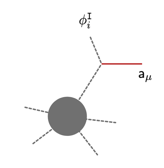
(a)   (b)

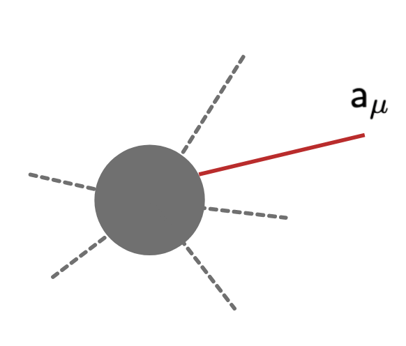
Figure 1: The leading soft factor of the $S$-matrix arise from diagrams where $\mathsf{a}_{\mu}$ is emitted from an external leg (figure-a above), while sub-leading soft factors arise from diagrams of both types (a) and (b).

Kinematics.

We denote all external hard momenta of $\phi^{\boldsymbol{\mathtt{I}}}_{i}$ as $p_{i}^{\mu}$, and the soft momenta of $\mathsf{a}_{\mu}$ as $k_{\mu}$. Here, the indices $i=1,\ldots,n$ are used to label the external particles. We can assume that the polarization tensors $\epsilon^{\boldsymbol{\mathtt{I}}}_{\mu(s)},\varepsilon_{\mu(s)},\tilde{\varepsilon}_{\mu(s)}$ are traceless,

$$\varphi^{\boldsymbol{\mathtt{I}}}_{\mu(s)} :\qquad \epsilon^{\boldsymbol{\mathtt{I}}\nu}{}_{\nu\mu(s-2)} =0\,,$$ (3.29a)

$$(A_{\mu(s)},\tilde{\mathsf{A}}_{\mu(s)}) :\qquad \varepsilon^{\,\nu}{}_{\nu\mu(s-2)} =0\,,\qquad\tilde{\varepsilon}^{\nu}{}_{\nu\mu(s-2)}=0\,,$$ (3.29b)

for all higher-spin modes $(\varphi^{i\boldsymbol{\mathtt{I}}}_{\mu(s)},A_{\mu(s)},\tilde{\mathsf{A}}_{\mu(s)})$. Moreover, they are also space-like

$$y^{\mu}\epsilon^{\boldsymbol{\mathtt{I}}}_{\mu\nu(s-1)}=0\,,\qquad y^{\mu}\varepsilon_{\mu\nu(s-1)}=0\,,\qquad y^{\mu}\tilde{\varepsilon}_{\mu\nu(s-1)}=0\,$$ (3.30)

as discussed above. These space-like gauge conditions play the role of the unitary or temporal gauge as in standard gauge theory; notice however that the $\mathfrak{hs}$ tensors are not automatically divergence-free and can be further decomposed into irreducible modes as discussed in [18, 15].

Gauge transformation.

Gauge transformations in the present framework are given by

$$\delta_{\xi}\mathsf{a}_{\mu}=\sum_{s}\{\underline{\mathtt{t}}_{\mu},\xi_{\nu(s)}u^{\nu(s)}\}\,,$$ (3.31)

where in the local $4d$ regime

$$\{\underline{\mathtt{t}}_{\mu},\xi_{\nu(s)}u^{\nu(s)}\}\approx\big{(}\sinh(\tau)\partial_{\mu}\xi_{\nu(s)}+s\tanh(\tau)y_{\mu}\xi_{\nu(s)}\big{)}u^{\nu(s)}\,.$$ (3.32)

This is precisely the gauge transformation one can use to gauge away the $\tilde{\zeta}$’s modes in (2.9) (see also [10]). At late time $\tau$, we can neglect the last term since $\lim_{\tau\rightarrow\infty}\tanh(\tau)=1$. Thus, to a very good approximation:

$$\{\underline{\mathtt{t}}_{\mu},\xi_{\nu(s)}\}\approx\sinh(\tau)\partial_{\mu}\xi_{\nu(s)}\,.$$ (3.33)

Hence, the gauge transformation for the $\mathfrak{hs}$-valued gauge field $\mathsf{a}_{\mu}$ in the $4d$ local regime reads

$$\delta_{\xi}\mathsf{a}_{\mu}\approx\sum_{s}\sinh(\tau)\partial_{\mu}\xi_{\nu(s)}u^{\nu(s)}\,.$$ (3.34)

As a result,

$$\delta_{\xi}\mathcal{V}_{3}=\sum_{s}\int\mho\,\sinh(\tau)^{2}\theta^{\rho\sigma}(\partial_{\rho}\phi_{\boldsymbol{\mathtt{I}}})(\partial_{\sigma}\partial^{\mu}\phi^{\boldsymbol{\mathtt{I}}})\partial_{\mu}\xi_{\nu(s)}u^{\nu(s)}\,.$$ (3.35)

This allows us to work purely with $\mathfrak{hs}$-valued functions $(\phi^{\boldsymbol{\mathtt{I}}}(y,u),\xi(y,u))$ when studying gauge invariance of the $S$-matrix in the soft limit. Upon integrating out $u$’s from (3.35), this boils down to the standard gauge transformation on spacetime

$$\delta_{\xi}A_{\mu(s)}=\partial_{\mu}\xi_{\mu(s-1)}\qquad\text{or}\qquad\delta_{\xi}\tilde{\mathsf{A}}_{\mu(s)}=\partial_{\mu}\xi_{\mu(s-1)}\ .$$ (3.36)

Soft factors in Lorentz-invariant field theory.

In general, the soft factors of $n$-point scattering amplitudes $\mathcal{M}_{n}$ are defined by

$$\mathcal{M}_{n+1}(p_{1},\ldots,p_{n};k)=\Big{(}\widetilde{\mathcal{S}}_{(\ell)}+\widetilde{\mathcal{S}}_{(\ell+1)}+\widetilde{\mathcal{S}}_{(\ell+2)}+\ldots\Big{)}\mathcal{M}_{n}(p_{1},\ldots,p_{n})\,$$ (3.37)

where $\ell$ is for leading, and

$$\widetilde{\mathcal{S}}_{(n)}=\sum_{i=1}^{n}\frac{f_{(n+1)}(k,\varepsilon,\tilde{\varepsilon};p_{i},J_{i},\epsilon_{i})}{k\cdot p_{i}}\,,\qquad J_{i}^{\mu\nu}:=p_{i}^{\mu}\frac{\partial}{\partial p_{i\nu}}-p_{i}^{\nu}\frac{\partial}{\partial p_{i\mu}}$$ (3.38)

is the soft factor of order $n$ in the soft momenta $k^{\mu}$ and $f_{(n+1)}$ are some functions of order $(n+1)$ in the soft momentum $k^{\mu}$. Here, $1/(k\cdot p_{i})$ is the propagator of the higher-spin fields $\varphi^{\boldsymbol{\mathtt{I}}}_{\mu(s)}$ linking $\mathcal{M}_{n}$ and the cubic vertices. Note that only the gauge fields need to be massless, while the $\mathfrak{hs}$-valued scalar fields can be massive in obtaining the above soft factors.

Imposing gauge invariance on the amplitudes, all soft theorems can be extracted from

$$\sum_{n\geq\ell}k_{\mu}\widetilde{\mathcal{S}}^{\mu\nu(s-1)}_{(n)}=0\,,$$ (3.39)

where $s$ denotes the spin of the emitting particle encoded in the $\mathfrak{hs}$-valued gauge field $\mathsf{a}_{\mu}$. Note that all sub-leading soft factors can be obtained by systematically trading each hard external momenta $p_{i}^{\mu}$ in $f_{(\ell+1)}(k,\varepsilon,\tilde{\varepsilon};p_{i},\epsilon_{i})$ for a factor of $k_{\nu}J_{i}^{\nu\mu}$ cf. [22, 23]. In deriving this result, all vertices in the standard quantum field theory approach are Lorentz-invariant. Moreover, since the angular momentum $J^{\mu\nu}$ is anti-symmetric, there is no need to go beyond $\widetilde{\mathcal{S}}_{(\ell+2)}$ to constrain the $S$-matrix due to the fact that $\widetilde{\mathcal{S}}_{(\ell+2)}$ is trivially gauge invariant due to symmetry. As such, $\widetilde{\mathcal{S}}_{(\ell)}$ and $\widetilde{\mathcal{S}}_{(\ell+1)}$ are usually all we need to determine IR physics. From this discussion, it is clear that once we obtain $\widetilde{\mathcal{S}}_{(\ell)}$, all soft theorems can be determined explicitly.

Soft limit in HS-IKKT scatterings.

We can now return to our setting where the cubic vertex (3.1) mildly violates Lorentz invariance and is not parity invariant. Let us consider a process where there are emission of a soft particle of fixed spin, say $s_{3}$, from the external legs of an $(n-1)$-point amplitude $\mathcal{M}_{n-1}$ (see diagram (a) in Fig 1). We will assume that the propagator, the external field and the soft emitting particle from $\mathcal{V}_{3}^{(s_{1},s_{2},s_{3})}$ carry momenta $\{p_{i}+k,p_{i};k\}$, respectively.

Considering a gauge transformation and plugging in plane-wave solutions to $\delta_{\xi}\mathcal{V}_{3}^{(s_{1},s_{2},s_{3})}$, we first observe that all terms come with the Levi-Civita symbols $\epsilon^{\mu\nu\rho\sigma}$ vanish due to symmetry in the soft limit. Furthermore:

$\bullet$ At $\Lambda=1$,

$$\delta_{\xi}\mathcal{V}_{3}^{(0,0,1)}=0\,$$ (3.40)

since the vertex vanishes identically. Hence, no constraint arises in this case.

$\bullet$ At $\Lambda=2$, non-trivial vertices are in (3.23). Let us consider (3.23c) as an example. The gauge transformation of this vertex results in,

$$\delta_{\xi}\mathcal{V}_{3}^{(0,0,2)}\approx L_{\rm NC}^{2}e^{-\frac{3}{2}\tau}\sum_{i}(p_{i}\cdot k)\Big{[}(E_{i}+k)p_{i}^{\alpha}-(p_{i}+k)^{\alpha}E_{i}\Big{]}\,.$$ (3.41)

where $E_{i}:=p_{i0}$ is the energy of the $i$th particle in the locally flat regime. As usual, the associated soft factor of the above can be obtained by dividing (3.41) with the propagator. Thus,

$$\widetilde{\mathcal{S}}_{(\ell)}[\mathcal{V}_{3}^{(0,0,2)}]\approx L_{\rm NC}^{2}e^{-\frac{3}{2}\tau}\sum_{i}\Big{[}(E_{i}+k)p_{i}^{\alpha}-(p_{i}+k)^{\alpha}E_{i}\Big{]}\,.$$ (3.42)

It is easy to see that, $\widetilde{\mathcal{S}}_{(\ell)}[\mathcal{V}_{3}^{(0,0,2)}]$ vanishes identically in the soft limit, i.e.

$$\lim_{k\rightarrow 0}\widetilde{\mathcal{S}}_{(\ell)}[\mathcal{V}_{3}^{(0,0,2)}]\approx L_{\rm NC}^{2}e^{-\frac{3}{2}\tau}\sum_{i}E_{i}\Big{[}p_{i}^{\mu}-p_{i}^{\mu}\Big{]}=0\,.$$ (3.43)

Therefore, no non-trivial constraints arise from the soft factors of the $S$-matrices. This is a direct consequence of the fact that the vertices of the matrix model are manifestly gauge invariant.

The story for cubic vertices with other higher-spin fields when $\Lambda\geq 4$ is completely analogous. Thus, the soft limit associated to the cubic vertex (3.1) in HS-IKKT simply provides the trivial relation (3.43). Notice that the above examples are consistent with the observation in [35] that the soft factors are tied to the number of derivatives in the interactions rather than spins.

As a final remark, we note that to have a local higher-spin theory with propagating degrees of freedom, one usually needs to abandon either unitarity as in the case of conformal higher-spin gravity [36, 37, 38, 39], or parity invariance as in the case of (quasi-) chiral higher-spin theories [40, 41, 42, 43, 44, 45, 46, 47, 48, 49]. Furthermore, it is also well-known that the construction of higher-spin theories using standard Noether couplings cannot surpass no-go theorems (see the discussion in Appendix C where we consider a non-commutative version of Noether couplings for higher-spin fields). However, in the present case of unitary Lorentzian HS-IKKT [15], the price to pay for a local higher-spin theory is somewhat different. Due to the presence of the cosmic vector field $\hat{\mathcal{Y}}$ in the cubic vertices, Lorentz invariance is not manifest, at least in the unitary formulation. This allows us to surpass the usual no-go theorems without sacrificing unitarity.

3.3 Some 3-point and 4-point higher-spin amplitudes

Since the HS-IKKT model on $\mathcal{M}^{1,3}$ contains Lorentz-violating interactions for the $\mathfrak{hs}$ modes, which include extra degrees of freedom corresponding to the would-be-massive modes, non-trivial 3-point scattering amplitudes do arise for the $\mathfrak{hs}$ modes. This statement can be justified by the fact that

$$p_{i}\cdot\epsilon_{i}\neq 0\,,\qquad k\cdot\varepsilon\neq 0\,,\qquad k\cdot\tilde{\varepsilon}\neq 0\,,$$ (3.44)

when fields are the would-be-massive modes and not divergence-free. However, in the massless limit where the fields are divergence-free, we have

$$p_{i}\cdot\epsilon_{i}=0\,,\qquad k\cdot\varepsilon=0\,,\qquad k\cdot\tilde{\varepsilon}=0\,,$$ (3.45)

so that all amplitudes vanish on-shell, in agreement with the standard story of QFT.

Let $\mathcal{M}_{3}^{(s_{1},s_{2},s_{3})}=\mathcal{M}_{3}(p_{1},\epsilon_{1},p_{2},\epsilon_{2};k_{3},\varepsilon_{3},\tilde{\varepsilon}_{3})$ be the 3-point amplitudes between two higher-spin fields $\varphi^{\boldsymbol{\mathtt{I}}}_{\mu(s)}$ and $\mathfrak{hs}$-valued gauge fields $A_{\mu\nu(s)}$ or $\tilde{\mathsf{A}}_{\nu(s-1)}$. One can check that

$\bullet$ At $\Lambda=1$, the 3-point amplitude vanishes $\mathcal{M}_{3}^{(0,0,1)}=0$.

$\bullet$ At $\Lambda=2$, we have

$$\mathcal{M}_{3}^{(1,0,1)} \sim\int d^{4}ye^{\mathrm{i}y\cdot(p_{1}+p_{2}+k_{3})}\Big{[}(y\cdot p_{1})(p_{2}\cdot\epsilon_{1})-(p_{1}\cdot\epsilon_{1})(y\cdot p_{2})\Big{]}(p_{2}\cdot\varepsilon_{3})-(1\leftrightarrow 2)\,,$$ (3.46a)

$$\mathcal{M}_{3}^{(0,1,1)} \sim\int d^{4}ye^{\mathrm{i}y\cdot(p_{1}+p_{2}+k_{3})}\Big{[}(y\cdot p_{1})(p_{2}\cdot\epsilon_{2})-(p_{1}\cdot\epsilon_{2})(y\cdot p_{2})\Big{]}(p_{2}\cdot\varepsilon_{3})-(1\leftrightarrow 2)\,,$$ (3.46b)

$$\mathcal{M}_{3}^{(0,0,2)} \sim\int d^{4}ye^{\mathrm{i}y\cdot(p_{1}+p_{2}+k_{3})}\Big{[}(y\cdot p_{1})(p_{2}^{\alpha}p_{2}^{\alpha}\varepsilon_{3\,\alpha(2)})-(p_{1}^{\alpha}p_{2}^{\alpha}\varepsilon_{3\,\alpha(2)})(y\cdot p_{2})\Big{]}-(1\leftrightarrow 2)\,,$$ (3.46c)

$$\widetilde{\mathcal{M}}_{3}^{(0,0,0)} \sim\int d^{4}ye^{\mathrm{i}y\cdot(p_{1}+p_{2}+k_{3})}\Big{[}(p_{1}\cdot p_{2})(y\cdot p_{2})\Big{]}-(1\leftrightarrow 2)=0\,.$$ (3.46d)

Note that the above expressions make sense in the local $4d$ regime at late times, where plane-wave solutions do exist, leading to the usual Dirac delta function $\delta^{4}(p_{1}+p_{2}+k_{3})$ corresponding to (local) momentum conservation. Moreover, when swapping the external legs, there is a minus sign coming from the original Poisson structure on $\mathbb{P}^{1,2}$ cf. (3.1). Treating $\hat{\mathcal{Y}}=y^{\mu}\partial_{\mu}\sim\cosh(\tau)\partial_{0}$, we get

$$\mathcal{M}_{3}^{(1,0,1)} \sim\delta^{4}(p_{1}+p_{2}+k_{3})\Big{[}E_{1}(p_{2}\cdot\epsilon_{1})-(p_{1}\cdot\epsilon_{1})E_{2}\Big{]}(p_{2}\cdot\varepsilon_{3})-(1\leftrightarrow 2)\,,$$ (3.47a)

$$\mathcal{M}_{3}^{(0,1,1)} \sim\delta^{4}(p_{1}+p_{2}+k_{3})\Big{[}E_{1}(p_{2}\cdot\epsilon_{2})-(p_{1}\cdot\epsilon_{2})E_{2}\Big{]}(p_{2}\cdot\varepsilon_{3})-(1\leftrightarrow 2)\,,$$ (3.47b)

$$\mathcal{M}_{3}^{(0,0,2)} \sim\delta^{4}(p_{1}+p_{2}+k_{3})\Big{[}E_{1}(p_{2}^{\alpha}p_{2}^{\alpha}\varepsilon_{3\,\alpha(2)})-(p_{1}^{\alpha}p_{2}^{\alpha}\varepsilon_{3\,\alpha(2)})E_{2}\Big{]}-(1\leftrightarrow 2)\,,$$ (3.47c)

$$\widetilde{\mathcal{M}}_{3}^{(0,0,0)} \sim 0\,.$$ (3.47d)

where $E_{i}:=p_{i0}$. All these 3-point amplitudes are suppressed by a factor of $L_{\rm NC}^{2}\,e^{-\frac{3}{2}\tau}$, which is not written explicitly.

As pointed out above, when external fields are would-be-massive modes, some of the above amplitudes are non-trivial. However, we notice that in the collinear limit where $p_{1}^{\mu}\propto p_{2}^{\mu}$, as well as the soft limit, all of the above amplitudes go to zero. This applies, in particular, to the on-shell massless modes. Furthermore, in the massless sector where fields are divergence-free, i.e. $p_{i}\cdot\epsilon_{i}=0$ and $k_{3}\cdot\varepsilon_{3}=0$ the above amplitudes also vanish.

$\bullet$ At $\Lambda=4$, we have for instance (explicit forms of all sub-vertices at $\Lambda=4$ can be found in Appendix B)

$$\mathcal{M}_{3}^{(0,0,4)} \sim 0\,,$$ (3.48a)

$$\widetilde{\mathcal{M}}_{3}^{(0,0,2)} \sim 0\,,$$ (3.48b)

etc. We refrain from exhibiting further 3-point scattering amplitudes for higher-spin fields and leave it as an exercise for enthusiastic readers. Note that it would be interesting to see how much the Lorentz-violating vertices considered in this work deviate from the standard Lorentz-invariant cubic vertices in $4d$ for massless/massive fields classified by Metsaev in the light-cone gauge [65].

Fusion rules.

Recall that the cubic vertex (3.1) only survives for $\Lambda\in 2\mathbb{N}^{+}$. The local $SO(3)$ invariance then leads to the following fusion rules or spin constraints

$$s_{3}\leq s_{1}+s_{2}+2\,,\qquad s_{1}\leq s_{2}+s_{3}+1\,,\qquad s_{2}\leq s_{1}+s_{3}+1\,$$ (3.49)

for $s_{1}+s_{2}+s_{3}=\Lambda\in 2\mathbb{N}^{+}$ and $s_{1},s_{2}\geq 0\,,\ s_{3}\geq 1$. This means that only a small number of exchange modes can occur when the external fields have low spins.

Four-point $\mathcal{M}_{4}(0,1,1,0)$ amplitude.

Let us apply the above fusion rules to study an explicit example of the 4-point amplitude $\mathcal{M}_{4}(0,1,1,0)$. This amplitude consists of $s$-, $t$-, $u$-channels and the contact interaction:

$$\mathcal{M}_{4}=\parbox{80.0pt}{\includegraphics[scale={0.25}]{s-channel}}+\parbox{60.0pt}{\includegraphics[scale={0.25}]{t-channel}}+\parbox{60.0pt}{\includegraphics[scale={0.25}]{u-channel}}+\parbox{80.0pt}{\includegraphics[scale={0.25}]{contact}}$$ (3.50)

where red denotes the external gauge fields and dash lines are scalar fields.

On the one hand, using the spin constraints (3.49), it follows that the only field that propagates in the exchange of the $s$- and $u$-channels in $\mathcal{M}_{4}(0,1,1,0)$ is $\varphi^{\boldsymbol{\mathtt{I}}}_{\mu}$. Indeed, we have $\mathcal{V}^{(s_{1}\geq 3,0,1)}=0$ and $\mathcal{V}^{(0,s_{2}\geq 3,1)}=0$ (see Appendix B). On the other hand, the $t$-channel receives contributions from the cubic vertices $\{\mathcal{V}_{3}^{(0,0,2)},\widetilde{\mathcal{V}}_{3}^{(0,0,0)}\}$, and the set of cubic vertices $\{\mathcal{U}_{3}^{(1,1,2)},\mathcal{U}_{3}^{(1,2,1)},\mathcal{U}_{3}^{(2,1,1)}\}$ as well as their descendants $\{\widetilde{\mathcal{U}}_{3}^{(1,1,0)},\widetilde{\mathcal{U}}_{3}^{(1,0,1)},\widetilde{\mathcal{U}}_{3}^{(0,1,1)}\}$.

Next, we also need the structure of the (quartic) contact term:

$$\mathcal{U}_{4}=\frac{1}{2}\int\mho\,\{\mathsf{a}^{\mu},\phi^{\boldsymbol{\mathtt{I}}}\}\{\mathsf{a}_{\mu},\phi_{\boldsymbol{\mathtt{I}}}\}=\frac{1}{2}\int\mho\,\theta^{\rho\sigma}\theta^{\alpha\beta}(\partial_{\rho}\mathsf{a}^{\mu}\partial_{\sigma}\phi^{\boldsymbol{\mathtt{I}}})(\partial_{\alpha}\mathsf{a}_{\mu}\partial_{\beta}\phi_{\boldsymbol{\mathtt{I}}})\,.$$ (3.51)

Using (A.2), we can average

$$[\theta^{\mu_{1}\nu_{1}}\theta^{\mu_{2}\nu_{2}}]_{0} \approx\frac{\ell_{p}^{2}R^{2}\sinh^{2}(\tau)}{3\cosh^{2}(\tau)}\Big{(}P^{\mu_{1}\mu_{2}}P^{\nu_{1}\nu_{2}}-P^{\mu_{1}\nu_{1}}P^{\nu_{1}\mu_{2}}\Big{)}\,,\qquad P^{\mu\nu}:=\eta^{\mu\nu}+\frac{y^{\mu}y^{\nu}}{R^{2}}\,.$$ (3.52)

This gives

$$\mathcal{U}_{4}^{(0,1,1,0)}\approx\frac{\ell_{p}^{2}R^{2}}{6}e^{-3\tau} \int\Bigg{(}\Big{[}(\partial_{\mu}\phi^{\boldsymbol{\mathtt{I}}})(\partial_{\nu}A^{\alpha})(\partial^{\mu}\phi_{\boldsymbol{\mathtt{I}}})(\partial^{\nu}A_{\alpha})-(\partial_{\mu}\phi^{\boldsymbol{\mathtt{I}}})(\partial_{\nu}A^{\alpha})(\partial^{\nu}\phi_{\boldsymbol{\mathtt{I}}})(\partial^{\mu}A_{\alpha})\Big{]}$$

$$+\frac{1}{R^{2}}\Big{[}(\hat{\mathcal{Y}}\phi^{\boldsymbol{\mathtt{I}}})(\partial_{\nu}A^{\alpha})(\hat{\mathcal{Y}}\phi_{\boldsymbol{\mathtt{I}}})(\partial^{\nu}A_{\alpha})+(\partial_{\mu}\phi^{\boldsymbol{\mathtt{I}}})(\hat{\mathcal{Y}}A^{\alpha})(\partial^{\mu}\phi_{\boldsymbol{\mathtt{I}}})(\hat{\mathcal{Y}}A_{\alpha})\Big{]}$$

$$-\frac{1}{R^{2}}\Big{[}(\hat{\mathcal{Y}}\phi^{\boldsymbol{\mathtt{I}}})(\partial_{\nu}A^{\alpha})(\partial^{\nu}\phi_{\boldsymbol{\mathtt{I}}})(\hat{\mathcal{Y}}A_{\alpha})+(\partial_{\mu}\phi^{\boldsymbol{\mathtt{I}}})(\hat{\mathcal{Y}}A^{\alpha})(\hat{\mathcal{Y}}\phi_{\boldsymbol{\mathtt{I}}})(\partial^{\mu}A_{\alpha})\Big{]}\Bigg{)}\,.$$ (3.53)

Since terms associated with the time-like vector field $\hat{\mathcal{Y}}$ are dominant, we can approximate the above to

$$\mathcal{U}_{4}^{(0,1,1,0)}\approx\frac{\ell_{p}^{2}}{6}e^{-3\tau}\int\Bigg{(} +\Big{[}(\hat{\mathcal{Y}}\phi^{\boldsymbol{\mathtt{I}}})(\partial_{\nu}A^{\alpha})(\hat{\mathcal{Y}}\phi_{\boldsymbol{\mathtt{I}}})(\partial^{\nu}A_{\alpha})+(\partial_{\mu}\phi^{\boldsymbol{\mathtt{I}}})(\hat{\mathcal{Y}}A^{\alpha})(\partial^{\mu}\phi_{\boldsymbol{\mathtt{I}}})(\hat{\mathcal{Y}}A_{\alpha})\Big{]}$$

$$-\Big{[}(\hat{\mathcal{Y}}\phi^{\boldsymbol{\mathtt{I}}})(\partial_{\nu}A^{\alpha})(\partial^{\nu}\phi_{\boldsymbol{\mathtt{I}}})(\hat{\mathcal{Y}}A_{\alpha})+(\partial_{\mu}\phi^{\boldsymbol{\mathtt{I}}})(\hat{\mathcal{Y}}A^{\alpha})(\hat{\mathcal{Y}}\phi_{\boldsymbol{\mathtt{I}}})(\partial^{\mu}A_{\alpha})\Big{]}\Bigg{)}\,.$$ (3.54)

where we have normalized $\mathcal{U}_{4}$ appropriately. Following the same line of argument as above, this quartic vertex is also suppressed in the late time regime. However, note that the quartic vertex is non-trivial even with the lowest possible external spins since $[\theta\theta]_{0}\neq 0$. Furthermore, unlike in Fronsdal-type higher-spin theories (see e.g. [66]), the quartic higher-spin vertices of Lorentzian HS-IKKT are local, at least in the unitary formulation. This remarkable property of the model allows us to use standard QFT techniques to compute the 4-point amplitudes, which are strongly suppressed.

The ingredients to compute the 4-point amplitude $\mathcal{M}_{4}(0,1,1,0)$, where external fields are positioned clock-wise, are summarized as follows:

• The propagators (3.12), (3.13) and (3.14) for $\varphi^{\boldsymbol{\mathtt{I}}}_{\alpha}$, $A_{\mu\nu}$ and $\tilde{\mathsf{A}}$, respectively.

• The cubic vertices $\{\mathcal{V}_{3}^{(0,1,1)}$,$\mathcal{V}_{3}^{(1,0,1)}$,$\mathcal{V}_{3}^{(0,0,2)}$, $\mathcal{U}_{3}^{(1,1,2)}$, $\mathcal{U}_{3}^{(1,2,1)}$, $\mathcal{U}_{3}^{(2,1,1)}\}$ and the descendants $\{\widetilde{\mathcal{V}}_{3}^{(0,0,0)},\widetilde{\mathcal{U}}_{3}^{(1,1,0)},\widetilde{\mathcal{U}}_{3}^{(1,0,1)},\mathcal{U}_{3}^{(0,1,1)}\}$. Their explicit forms can be found in Subsection 3.1.

• The quartic vertex $\mathcal{U}_{4}^{(0,1,1,0)}$.

Explicitly, the individual contributions to $\mathcal{M}_{4}(0,1,1,0)$ are as follows:

$\bullet$ $s$-channel:

$$\mathcal{M}_{s}\approx\frac{L^{4}_{\rm NC}}{9s}e^{-3\tau}\Big{(} +2(p_{1}\cdot\epsilon_{2})\big{[}E_{1}p_{2}^{\alpha}-E_{2}p_{1}^{\alpha}\big{]}+(p_{2}\cdot\epsilon_{2})\big{[}E_{1}p_{2}^{\alpha}-E_{2}p_{1}^{\alpha}\big{]}\Big{)}$$

$$\times\hat{\kappa}_{\alpha\beta}\Big{(} +2(p_{4}\cdot\epsilon_{3})\big{[}E_{4}p_{3}^{\beta}-E_{3}p_{4}^{\beta}\big{]}+(p_{3}\cdot\epsilon_{3})\big{[}E_{4}p_{3}^{\beta}-E_{3}p_{4}^{\beta}\big{]}\Big{)}\,.$$ (3.55)

$\bullet$ $t$-channel:

$$\mathcal{M}_{t}\approx +\frac{L_{\rm NC}^{4}}{9t}e^{-3\tau}\Big{(}+(p_{2}\cdot\epsilon_{3})\epsilon_{2}^{\nu}\big{[}E_{2}p_{3}^{\zeta}-E_{3}p_{2}^{\zeta}\big{]}+(\epsilon_{2}\cdot\epsilon_{3})p_{2}^{\nu}\big{[}E_{3}p_{2}^{\nu}-E_{2}p_{3}^{\nu}\big{]}$$

$$\qquad\qquad+\big{[}(p_{2}+p_{3})\cdot\epsilon_{2}\big{]}\epsilon_{3}^{\nu}\big{[}E_{3}p_{2}^{\nu}-E_{2}p_{3}^{\nu}\big{]}-(2\leftrightarrow 3)\Big{)}$$

$$\qquad\qquad\times(\hat{\kappa}_{\zeta\alpha}\hat{\kappa}_{\nu\beta}+\hat{\kappa}_{\zeta\beta}\hat{\kappa}_{\nu\alpha})\Big{(}\big{[}E_{1}p_{4}^{\alpha}-E_{4}p_{1}^{\alpha}\big{]}p_{4}^{\beta}-(1\leftrightarrow 4)\Big{)}$$

$$+\frac{L_{\rm NC}^{4}}{9t}e^{-3\tau}\Big{(}E_{2}\big{[}(p_{2}\cdot\epsilon_{3})(p_{3}\cdot\epsilon_{2})-(p_{2}\cdot p_{3})(\epsilon_{2}\cdot\epsilon_{3})-(p_{2}\cdot\epsilon_{2})(p_{3}\cdot\epsilon_{3})-(p_{3}\cdot\epsilon_{2})(p_{3}\cdot\epsilon_{3})\big{]}$$

$$\qquad\qquad\quad+E_{3}\big{[}(p_{2}\cdot\epsilon_{3})(p_{2}\cdot\epsilon_{3})+(p_{2}\cdot\epsilon_{2})(p_{3}\cdot\epsilon_{2})-(p_{2}\cdot\epsilon_{2})(p_{2}\cdot\epsilon_{3})\big{]}-(2\leftrightarrow 3)\Big{)}$$

$$\qquad\qquad\times\Big{(}E_{4}(p_{1}\cdot p_{4})-(1\leftrightarrow 4)\Big{)}\,.$$ (3.56)

$\bullet$ $u$-channel:

$$\mathcal{M}_{u}\approx\frac{L^{4}_{\rm NC}}{9u\,}e^{-3\tau}\Big{(} +2(p_{1}\cdot\epsilon_{3})\big{[}E_{1}p_{3}^{\alpha}-E_{3}p_{1}^{\alpha}\big{]}+(p_{3}\cdot\epsilon_{3})\big{[}E_{1}p_{3}^{\alpha}-E_{3}p_{1}^{\alpha}\big{]}\Big{)}$$

$$\times\hat{\kappa}_{\alpha\beta}\Big{(} +2(p_{4}\cdot\epsilon_{2})\big{[}E_{4}p_{2}^{\beta}-E_{2}p_{4}^{\beta}\big{]}+(p_{2}\cdot\epsilon_{2})\big{[}E_{4}p_{2}^{\beta}-E_{2}p_{4}^{\beta}\big{]}\Big{)}\,.$$ (3.57)

$\bullet$ contact term:

$$\mathcal{M}_{c} \approx\frac{L_{\rm NC}^{4}}{6}e^{-3\tau}\Bigg{[}(\epsilon_{2}\cdot\epsilon_{3})\Big{(}(p_{2}\cdot p_{3})(E_{1}E_{4}+E_{2}E_{3})-(p_{1}\cdot p_{3})(E_{1}E_{3}+E_{2}E_{4})\Big{)}\pm\binom{1\leftrightarrow 4}{2\leftrightarrow 3}\Bigg{]}\,.$$ (3.58)

Here $(s,t,u)$ are the standard Mandelstam variables, and we recall that all $\hat{\kappa}_{\mu\nu}$ tensors in the above expressions are space-like cf. (3.8). In addition, we have suppressed the overall Dirac delta function for momentum conservation, and used $\hat{\mathcal{Y}}\sim\cosh(\tau)\partial_{0}$ as above. Again, we note that even though the above contributions to the 4-point amplitudes $\mathcal{M}_{4}(0,1,1,0)$ in Lorentzian HS-IKKT are non-trivial, they are strongly suppressed in the late time regime.

3.4 Covariant higher-spin fields and gravitational couplings

So far, we used the space-like representation (2.8) of fields, which is useful for amplitude calculations but obscures Lorentz invariance. This subsection briefly discusses the covariant representation of higher-spin fields on $\mathcal{M}^{1,3}$. In particular, we will consider the gravitational coupling between a covariant graviton and two scalar fields given by (3.1), which looks rather strange in the space-like formulation. We will see that such vertices can be rewritten in a perfectly standard form using the covariant representation.

Covariant higher-spin fields.

We have seen that the space-like realization of the $\mathfrak{hs}$-valued fields interact via Lorentz-violating vertices. On the other hand, the same degrees of freedom can also be represented in a more conventional form in terms of “covariant” rank $s$ Fronsdal-like tensor fields, which have the form

$$\Phi^{\boldsymbol{\mathtt{I}}}_{\mu(s)}=\{y_{\mu_{1}},\{\ldots\{y_{\mu_{s}},\phi^{\boldsymbol{\mathtt{I}}}_{(s)}\}\ldots\}\}\big{|}_{0}$$ (3.59)

where $\phi^{\boldsymbol{\mathtt{I}}}_{(s)}:=\varphi^{\boldsymbol{\mathtt{I}}}_{\nu(s)}u^{\nu(s)}$ arises from transversal matrices. Here $\Phi^{\boldsymbol{\mathtt{I}}}_{\mu(s)}$ are totally symmetric divergence-free tensor fields which are no longer space-like, i.e. [20]

$$0=\partial_{\mu}(\rho_{M}\Phi^{\mu\nu(s-1)})\,,\quad\partial_{\mu}:=\eth_{\mu}-\frac{y_{\mu}}{y_{4}}\eth_{4}\,,\quad\eth^{a}f(y):=-\frac{1}{\ell_{p}^{2}R^{2}}\theta^{ab}\{y_{b},f(y)\}\,$$ (3.60)

cf. (2.19). Here $a=0,1,\ldots,4$ are indices of the $SO(1,4)$ algebra that defines $H^{4}_{N}$, $\rho_{M}=(\sinh(\tau))^{-1}$ and $\partial_{\mu}y^{\nu}=\delta_{\mu}{}^{\nu}$. We restrict ourselves to the local physical regime where

$$\theta^{\mu\nu}\approx\ell_{p}^{2}(y^{\mu}u^{\nu}-y^{\nu}u^{\mu})\,$$ (3.61)

using $\cosh(\tau)\sim\sinh(\tau)$ for $\tau\rightarrow\infty$. In this regime, $\{y_{\mu},-\}$ acts trivially on the $u$ generators, so that the covariant higher-spin fields $\Phi^{\boldsymbol{\mathtt{I}}}_{\mu(s)}$ are obtained using (2.5) as

$$\Phi^{\boldsymbol{\mathtt{I}}}_{\mu(s)}\approx\big{[}\theta_{\mu_{1}}{}^{\sigma_{1}}\ldots\theta_{\mu_{s}}{}^{\sigma_{s}}u^{\nu_{1}}\ldots u^{\nu_{s}}\big{]}_{0}\partial_{\sigma_{1}}\ldots\partial_{\sigma_{s}}\varphi^{\boldsymbol{\mathtt{I}}}_{\nu(s)}\ .$$ (3.62)

It can be checked that $\partial^{\mu}\Phi^{\boldsymbol{\mathtt{I}}}_{\mu\nu(s-1)}=0$. This provides a map from the space-like formulation to the covariant formulation of $\mathfrak{hs}$ fields in Lorentzian HS-IKKT theory.

To illustrate the relevance of the above covariant tensors, consider again the case of spin 2 fluctuations arising from the first higher-spin mode of $\mathsf{a}_{\mu}$, i.e.

$$\mathsf{a}_{\mu}^{(1)}=\mathcal{A}_{\mu|\nu}(y)u^{\nu}\ .$$ (3.63)

This determines the following “covariant” would-be-massive graviton [18]

$$h^{\mu\nu} =\{y^{\mu},\mathsf{a}^{\nu}_{(1)}\}+\{y^{\nu},\mathsf{a}^{\mu}_{(1)}\}$$

$$\approx\frac{\ell_{p}}{3}\Big{[}y^{\mu}\partial_{\rho}\mathcal{A}^{\nu|\rho}+y^{\nu}\partial_{\rho}\mathcal{A}^{\mu|\rho}-\hat{\mathcal{Y}}\big{(}\mathcal{A}^{\mu|\nu}+\mathcal{A}^{\nu|\mu}\big{)}\Big{]}+\ell_{p}\big{(}\mathcal{A}^{\mu|\nu}+\mathcal{A}^{\nu|\mu}\big{)}$$

$$\approx\frac{\ell_{p}}{3}\Big{[}y^{\mu}\partial_{\rho}A^{\nu\rho}+y^{\nu}\partial_{\rho}A^{\mu\rho}+y^{\mu}\partial^{\nu}f+y^{\nu}\partial^{\mu}f-2\hat{\mathcal{Y}}\big{(}A^{\mu\nu}+\eta^{\mu\nu}f\big{)}\Big{]}+2\ell_{p}\Big{[}A^{\mu\nu}+\eta^{\mu\nu}f\Big{]}$$ (3.64)

projecting along the fiber. Note that the terms in the first square bracket dominate. Thus, to a very good approximation

$$h^{\mu\nu}\approx\frac{L_{\rm NC}^{2}}{R\cosh(\tau)}\Big{[}y^{\mu}\partial_{\rho}A^{\nu\rho}+y^{\nu}\partial_{\rho}A^{\mu\rho}+y^{\mu}\partial^{\nu}f+y^{\nu}\partial^{\mu}f-2\hat{\mathcal{Y}}\big{(}A^{\mu\nu}+\eta^{\mu\nu}f\big{)}\Big{]}$$ (3.65)

in the late time regime. This illustrates the field redefinition relating the unitary and covariant representation of the same $\mathfrak{hs}$ degrees of freedom. It is not hard to see that $h^{\mu\nu}$ transforms under gauge transformations as [15]

$$h_{\mu\nu}\to h_{\mu\nu}+\partial_{\mu}\xi_{\nu}\ +\partial_{\nu}\xi_{\mu}$$ (3.66)

in the flat limit, where $\xi^{\mu}=\{\Lambda,y^{\mu}\}$ is a divergence-free vector field generated by the gauge parameter $\Lambda$ [67]. The underlying gauge group consists of volume-preserving diffeomorphism in space-time, and $\mathfrak{hs}$-valued generalizations thereof arising from symplectic vector fields on the underlying twistor space $\mathbb{P}^{1,2}$. This contains in particular all Lorentz transformations around any given point. In that way, the appropriate action of Lorentz transformations arises for the tensor indices, which is not the case in the unitary formulation for $\mathfrak{hs}$ modes. These observations strongly suggest that Lorentz invariance should effectively hold in the theory when we work with the covariant representation. This will be seen explicitly below. However, the inverse of the map (3.59) amounts to a non-local field redefinition, cf. [15]. Hence, in the covariant formalism, the action will be non-local if higher-spin fields are involved. This suggests the following interesting picture:

Lorentzian HS-IKKT theory can be viewed either as local and unitary but mildly Lorentz-violating, or as Lorentz invariant but mildly non-local.

$\mathfrak{hs}$-valued gravitational coupling.

Using the above covariant graviton $h_{\mu\nu}$ in the local 4-dimensional regime, we can rewrite the vertex (3.1) in terms of a coupling between a $\mathfrak{hs}$-valued graviton $h_{\mu\nu}$ and two $\mathfrak{hs}$-valued scalar fields as follows:

$$\mathcal{V}(\phi^{\boldsymbol{\mathtt{I}}}_{(s_{1})},\phi_{\boldsymbol{\mathtt{I}}}^{(s_{2})},\mathsf{a}^{(s_{3})}) =\int\mho\,\{\underline{\mathtt{t}}^{\mu},\phi^{\boldsymbol{\mathtt{I}}}_{(s_{1})}\}\{\phi_{\boldsymbol{\mathtt{I}}}^{(s_{2})},\mathsf{a}_{\mu}^{(s_{3})}\}\approx e^{-\frac{3}{2}\tau}\int d^{4}y\,\partial^{\mu}\phi^{\boldsymbol{\mathtt{I}}}_{(s_{1})}\partial^{\nu}\phi_{\boldsymbol{\mathtt{I}}}^{(s_{2})}\{y_{\nu},\mathsf{a}_{\mu}^{(s_{3})}\}$$

$$\approx e^{-\frac{3}{2}\tau}\int d^{4}y\,\partial_{\mu}\phi^{\boldsymbol{\mathtt{I}}}_{(s_{1})}\partial_{\nu}\phi_{\boldsymbol{\mathtt{I}}}^{(s_{2})}h^{\mu\nu}_{(s_{3})}\,.$$ (3.67)

This is similar to the standard, minimal gravitational coupling between a covariant graviton and two scalar fields, cf. (3.20c). The vertex now looks perfectly covariant, even though all fields are $\mathfrak{hs}$-valued. Notice also the absence of the non-commutativity scale $L_{\rm NC}$ in this formalism. Similarly, we can write the quartic vertex (3.51) as

$$\mathcal{V}(\phi^{\boldsymbol{\mathtt{I}}}_{(s_{1})},\mathsf{a}^{(s_{2})},\phi_{\boldsymbol{\mathtt{I}}}^{(s_{3})},\mathsf{a}_{(s_{4})}) =\int\mho\,\{\phi^{\boldsymbol{\mathtt{I}}}_{(s_{1})},\mathsf{a}^{\mu}_{(s_{2})}\},\{\phi_{\boldsymbol{\mathtt{I}}}^{(s_{3})},\mathsf{a}_{\mu}^{(s_{4})}\}$$

$$\approx e^{-3\tau}\int d^{4}y\,\partial^{\rho}\phi^{\boldsymbol{\mathtt{I}}}_{(s_{1})}h_{\mu\rho}^{(s_{2})}\partial^{\sigma}\phi_{\boldsymbol{\mathtt{I}}}^{(s_{3})}h^{\mu}{}_{\sigma(s_{4})}\,.$$ (3.68)

Note that the higher-spin valued graviton $h_{\mu\nu}$ is not fundamental, but rather arises as derivative of the underlying space-like tensor field $\mathcal{A}_{\mu|\nu(s)}(y)$. This is typical for Yang-Mills theories, where the physical fields are given as derivations of some potentials. The same observation also applies to the full $\mathfrak{hs}$-valued fluctuation mode $\mathsf{a}_{\mu}$ as shown above. This illustrates how the strange-looking vertices in Section 3.1 can be reconciled with the conventional, covariant language of QFT, and Lorentz invariance is recovered at least for some vertices.

Using the gauge transformation (3.66), it can be checked immediately that the gravitational cubic vertex (3.4) obeys the standard Weinberg’s soft theorem for low energy graviton

$$\sum_{i}p_{i}^{\mu}=0\,$$ (3.69)

due to momentum conservation. In addition, the 3-point amplitude of (3.4) reads

$$\mathcal{M}_{3}\sim\delta^{4}(p_{1}+p_{2}+k_{3})e^{-\frac{3}{2}\tau}(p_{1\mu}p_{2\nu}\varepsilon_{3}^{\mu\nu})+(1\leftrightarrow 2)\,,$$ (3.70)

which is non-trivial if the fields are would-be-massive modes.

$\mathfrak{hs}$-valued Yang-Mills action.

Finally, we briefly comment on an analogous covariant form of the cubic vertices (3.26) for the gauge fields, and their quartic generalization. These are part of the Yang-Mills term in the action, which does admit a covariant formulation along the lines of [68]. Viewing the 3+1 semi-classical matrices $t^{\mu}=\underline{\mathtt{t}}^{\mu}+\mathsf{a}^{\mu}(y|u)$ as $\mathfrak{hs}$-valued functions on $\mathcal{M}^{1,3}$ in the local coordinates $y^{\mu}$, the Yang-Mills term of the action can be written in the local 4-dimensional regime as $S_{\rm YM}\sim\int_{\mathcal{M}}\,\mathcal{L}_{\rm YM}$ with

$$\mathcal{L}_{\rm YM}:=\{t^{\mu},t^{\nu}\}\{t_{\mu},t_{\nu}\}=\gamma^{\mu\nu}\gamma^{\rho\sigma}\mathsf{F}_{\mu\rho}\mathsf{F}_{\nu\sigma}\ .$$ (3.71)

Here, $\mathsf{F}_{\mu\rho}$ is a $\mathfrak{hs}$-valued generalization of the symplectic form on $\mathcal{M}^{1,3}$, and $\gamma^{\mu\nu}$ is the effective metric whose fluctuations are given by the graviton $h^{\mu\nu}$ (3.4). All of these are tensorial objects transforming nicely under gauge transformations. This strongly suggests that the associated interaction vertices should also transform covariantly under gauge transformation, and therefore respect Lorentz invariance in some form similar to the above.

4 Discussion

In this work, we studied the fate of soft theorems of the Lorentzian HS-IKKT model on a FLRW cosmological spacetime $\mathcal{M}^{1,3}$. Our results show that Lorentzian HS-IKKT theory leads to non-trivial higher-spin scattering, due to the fact that the vertices are mildly Lorentz- and parity-violating in the space-like formulation.

To illustrate these results, we computed explicitly some 3-point scattering amplitudes in the space-like formulation of Lorentzian HS-IKKT. The amplitudes for the would-be-massive modes are non-trivial, but are strongly suppressed at low energies and in the weak curvature regime. In the massless sector, the amplitudes vanish on-shell. We also obtained the fusion rules for some cubic vertices with higher-spin fields in Lorentzian HS-IKKT, e.g. the couplings between two $\mathfrak{hs}$-valued scalar fields with a $\mathfrak{hs}$-valued gauge field. As an example, we study the simplest 4-point amplitude $\mathcal{M}_{4}(0,1,1,0)$ with two scalars and two gauge fields $A_{\mu}$ on the external legs, which is strongly suppressed as expected.

To carry out these computations, we use two different ways of organizing the $\mathfrak{hs}$ modes of the model: The first, “space-like” or unitary representation makes the physical degrees of freedom very explicit, at the expense of manifest covariance. The second, “covariant” formulation is closer to the standard formulation of Fronsdal-like higher-spin fields, but involves a non-trivial and non-local field redefinition. This formulation allows us to recast at least some space-like vertices in standard, covariant form. Then Lorentz invariance is effectively recovered at least for some sector of the theory, at the expense of manifest locality.

Our results provide further evidence that the higher-spin gauge theory induced by the IKKT matrix model on the present cosmological background is a consistent theory with physically reasonable and perhaps near-realistic features.

There are many interesting directions for future work on this model. One obvious problem is to extend the present study to the non-abelian case, where higher-spin gauge fields take values in the $\mathfrak{su}(n)$ Lie algebra. Another interesting project is to find a global spinorial formulation for Lorentzian HS-IKKT on $\mathcal{M}^{1,3}$. In particular, the approach in [10] based on spinors transforming under the compact space-like subgroup $SU(2)_{L}\times SU(2)_{R}\subset SU(2,2)$ is of limited use in the Lorentzian setting. To resolve this issue, one may try to consider the rotation subgroup to be the space-like isometry group $SL(2,\mathbb{C})\simeq SO(1,3)$ where we can define Weyl spinors on $H^{4}$. This will be addressed in future work.

On the conceptual side, one important problem is to understand better the fate of Lorentz invariance, which is not manifest in the space-like/unitary formulation for higher-spin fields. Since the theory is invariant under $\mathfrak{hs}$-valued volume-preserving diffeomorphism, Lorentz invariance is expected to hold effectively in some sense. We have seen that this can be made manifest for some fields and vertices in the covariant formulation, and a more general understanding of this issue would be very important.

Finally, as advertised in the introduction, a modified version of GR arises from quantum effects of the IKKT matrix model, as demonstrated in the one-loop effective action [5]. The observed exponential suppression of the interaction vertices provides further justification for the weak coupling approach underlying that computation. Moreover, the present results suggest studying the loop amplitude of HS-IKKT theory using similar methods as in the present paper.

Appendix A Useful relations

This appendix provides additional relations for $\mathcal{M}^{1,3}$ used in the main text. All the relations here are extracted from [9, 15, 18]. Let $y_{a}$ for $a=0,1,2,3,4$ be coordinates of $H^{4}$ where $y_{a}y^{a}=-R^{2}$ and $y^{a}$ transform as vectors under $SO(1,4)$ with generator $m^{ab}$. After projecting out $y^{4}=R\sinh(\tau)$, we have the following relations

$$y_{\mu}\underline{\mathtt{t}}^{\mu} =0\,,\qquad\qquad\qquad\qquad\quad\quad\qquad\qquad\qquad\quad\ \ \mu=0,1,2,3\,,$$ (A.1a)

$$\eta_{\mu\nu}\underline{\mathtt{t}}^{\mu}\underline{\mathtt{t}}^{\nu} =\frac{1}{\ell_{p}^{2}}+\frac{y_{4}^{2}}{\ell_{p}^{2}R^{2}}=+\ell_{p}^{-2}\cosh^{2}(\tau)\,,\qquad\qquad\quad\ \eta_{\mu\nu}=\,\mathrm{diag}(-,+,+,+)\,,$$ (A.1b)

$$y^{\mu}y_{\mu} =-R^{2}\cosh^{2}(\tau)$$ (A.1c)

$$\{\underline{\mathtt{t}}^{\mu},y^{\nu}\} =+\frac{\eta^{\mu\nu}}{R}y^{4}=\eta^{\mu\nu}\sinh(\tau)\,,$$ (A.1d)

$$\{\underline{\mathtt{t}}^{\mu},y^{4}\} =-\frac{y^{\mu}}{R}\,,$$ (A.1e)

$$m^{\mu\nu} =-\frac{\theta^{\mu\nu}}{\ell_{p}^{2}}=-\frac{1}{\cosh^{2}(\tau)}\Big{(}\sinh(\tau)(y^{\mu}\underline{\mathtt{t}}^{\nu}-y^{\nu}\underline{\mathtt{t}}^{\mu})+\epsilon^{\mu\nu\sigma\rho}y_{\sigma}\underline{\mathtt{t}}_{\rho}\Big{)}\,,$$ (A.1f)

which are frequently used in the main text. Note that in the local physical regime

$$\theta^{\mu\nu}\approx\frac{\ell_{p}\sinh(\tau)}{\cosh(\tau)}(y^{\mu}u^{\nu}-y^{\nu}u^{\mu})\,.$$ (A.2)

Appendix B Vertices at $\Lambda=4$

This appendix derives all sub-vertices of (3.1) at $\Lambda=4$, where

$$\mathcal{V}_{3}^{[4]}= +\mathcal{V}^{(0,0,4)}_{3}+\mathcal{V}_{3}^{(1,0,3)}+\mathcal{V}_{3}^{(0,1,3)}+\mathcal{V}_{3}^{(0,2,2)}+\mathcal{V}_{3}^{(2,0,2)}+\mathcal{V}_{3}^{(1,1,2)}$$

$$+\mathcal{V}_{3}^{(2,1,1)}+\mathcal{V}_{3}^{(1,2,1)}+\mathcal{V}_{3}^{(3,0,1)}+\mathcal{V}_{3}^{(0,3,1)}\,.$$ (B.1)

Below, the pre-factors of all sub-vertices $\mathcal{V}_{3}^{(s_{1},s_{2},s_{3})}$ is $\frac{2\ell_{p}}{27\cosh(\tau)\sqrt{\sinh(\tau)}}$. We will suppress this factor to simplify our expressions.

Firstly, due to tracelessness

$$\mathcal{V}_{3}^{(0,0,4)} \sim 0\,,$$

$$\widetilde{\mathcal{V}}_{3}^{(0,0,2)} \sim 0\,.$$

Next, we have

$$\mathcal{V}_{3}^{(1,0,3)} \sim\int\Big{[}(\hat{\mathcal{Y}}\varphi_{\boldsymbol{\mathtt{I}}}^{\alpha_{3}})(\partial^{\alpha_{2}}\partial^{\mu}\phi^{\boldsymbol{\mathtt{I}}})-(\partial^{\alpha_{2}}\varphi_{\boldsymbol{\mathtt{I}}}^{\alpha_{3}})(\hat{\mathcal{Y}}\partial^{\mu}\phi^{\boldsymbol{\mathtt{I}}})\Big{]}A_{\mu\alpha_{2}\alpha_{3}}+\frac{y_{\beta}\epsilon^{\beta\alpha_{2}\rho\sigma}}{\sinh(\tau)}(\partial_{\rho}\varphi_{\boldsymbol{\mathtt{I}}}^{\alpha_{3}})(\partial_{\sigma}\partial^{\mu}\phi^{\boldsymbol{\mathtt{I}}})A_{\mu\alpha_{2}\alpha_{3}}\,,$$

$$\mathcal{V}_{3}^{(0,1,3)} \sim\int\Big{[}(\hat{\mathcal{Y}}\phi_{\boldsymbol{\mathtt{I}}})(\partial^{\alpha_{2}}\partial^{\mu}\varphi^{\boldsymbol{\mathtt{I}}\alpha_{3}})-(\partial^{\alpha_{2}}\phi_{\boldsymbol{\mathtt{I}}})(\hat{\mathcal{Y}}\partial^{\mu}\varphi^{\boldsymbol{\mathtt{I}}\alpha_{3}})\Big{]}A_{\mu\alpha_{2}\alpha_{3}}+\frac{y_{\beta}\epsilon^{\beta\alpha_{2}\rho\sigma}}{\sinh(\tau)}(\partial_{\rho}\phi_{\boldsymbol{\mathtt{I}}})(\partial_{\sigma}\partial^{\mu}\varphi^{\boldsymbol{\mathtt{I}}\alpha_{3}})A_{\mu\alpha_{2}\alpha_{3}}\,.$$

The descendant vertices associated with the above are

$$\widetilde{\mathcal{V}}_{3}^{(1,0,1)} \sim\int\Big{[}(\hat{\mathcal{Y}}\varphi_{\boldsymbol{\mathtt{I}}}^{\alpha_{3}})(\Box\phi^{\boldsymbol{\mathtt{I}}})-(\partial_{\mu}\varphi_{\boldsymbol{\mathtt{I}}}^{\alpha_{3}})(\hat{\mathcal{Y}}\partial^{\mu}\phi^{\boldsymbol{\mathtt{I}}})\Big{]}\tilde{\mathsf{A}}_{\alpha_{3}}+\Big{[}(\hat{\mathcal{Y}}\varphi_{\boldsymbol{\mathtt{I}}\mu})(\partial^{\alpha_{2}}\partial^{\mu}\phi^{\boldsymbol{\mathtt{I}}})-(\partial^{\alpha_{2}}\varphi_{\boldsymbol{\mathtt{I}}\mu})(\hat{\mathcal{Y}}\partial^{\mu}\phi^{\boldsymbol{\mathtt{I}}})\Big{]}\tilde{\mathsf{A}}_{\alpha_{2}}$$

$$\qquad+\int\frac{y_{\beta}\epsilon^{\beta\alpha_{2}\rho\sigma}}{\sinh(\tau)}(\partial_{\rho}\varphi_{\boldsymbol{\mathtt{I}}\mu})(\partial_{\sigma}\partial^{\mu}\phi^{\boldsymbol{\mathtt{I}}})\tilde{\mathsf{A}}_{\alpha_{2}}\,,$$

$$\widetilde{\mathcal{V}}_{3}^{(0,1,1)} \sim\int\Big{[}(\hat{\mathcal{Y}}\phi_{\boldsymbol{\mathtt{I}}})(\Box\varphi^{\boldsymbol{\mathtt{I}}\alpha_{3}})-(\partial_{\mu}\phi_{\boldsymbol{\mathtt{I}}})(\hat{\mathcal{Y}}\partial^{\mu}\varphi^{\boldsymbol{\mathtt{I}}\alpha_{3}})\Big{]}\tilde{\mathsf{A}}_{\alpha_{3}}+\Big{[}(\hat{\mathcal{Y}}\phi_{\boldsymbol{\mathtt{I}}})(\partial^{\alpha_{2}}\partial^{\mu}\varphi_{\boldsymbol{\mathtt{I}}\mu})-(\partial^{\alpha_{2}}\phi_{\boldsymbol{\mathtt{I}}})(\hat{\mathcal{Y}}\partial^{\mu}\varphi^{\boldsymbol{\mathtt{I}}}_{\mu})\Big{]}\tilde{\mathsf{A}}_{\alpha_{2}}$$

$$\qquad+\int\frac{y_{\beta}\epsilon^{\beta\alpha_{2}\rho\sigma}}{\sinh(\tau)}(\partial_{\rho}\phi_{\boldsymbol{\mathtt{I}}})(\partial_{\sigma}\partial_{\mu}\varphi^{\boldsymbol{\mathtt{I}}\mu})\tilde{\mathsf{A}}_{\alpha_{2}}\,.$$

Similarly, we get

$$\mathcal{V}_{3}^{(0,2,2)} \sim\int\Big{[}(\hat{\mathcal{Y}}\phi_{\boldsymbol{\mathtt{I}}})(\partial^{\alpha_{1}}\partial^{\mu}\varphi^{\boldsymbol{\mathtt{I}}}_{\alpha_{1}\alpha_{2}})-(\partial^{\alpha_{1}}\phi_{\boldsymbol{\mathtt{I}}})(\hat{\mathcal{Y}}\partial^{\mu}\varphi^{\boldsymbol{\mathtt{I}}}_{\alpha_{1}\alpha_{2}})\Big{]}A_{\mu}{}^{\alpha_{2}}+\frac{y_{\beta}\epsilon^{\beta\alpha_{1}\rho\sigma}}{\sinh(\tau)}(\partial_{\rho}\phi_{\boldsymbol{\mathtt{I}}})(\partial_{\sigma}\partial^{\mu}\varphi^{\boldsymbol{\mathtt{I}}}_{\alpha_{1}\alpha_{2}})A_{\mu}{}^{\alpha_{2}}\,,$$

$$\mathcal{V}_{3}^{(2,0,2)} \sim\int\Big{[}(\hat{\mathcal{Y}}\varphi_{\boldsymbol{\mathtt{I}}\alpha_{1}\alpha_{2}})(\partial^{\alpha_{1}}\partial^{\mu}\phi^{\boldsymbol{\mathtt{I}}})-(\partial^{\alpha_{1}}\varphi_{\boldsymbol{\mathtt{I}}\alpha_{1}\alpha_{2}})(\hat{\mathcal{Y}}\partial^{\mu}\phi^{\boldsymbol{\mathtt{I}}})\Big{]}A_{\mu}{}^{\alpha_{2}}+\frac{y_{\beta}\epsilon^{\beta\alpha_{1}\rho\sigma}}{\sinh(\tau)}(\partial_{\rho}\varphi_{\boldsymbol{\mathtt{I}}\alpha_{1}\alpha_{2}})(\partial_{\sigma}\partial^{\mu}\phi^{\boldsymbol{\mathtt{I}}})A_{\mu}{}^{\alpha_{2}}\,,$$

$$\mathcal{V}_{3}^{(1,1,2)} \sim\frac{1}{2}\Bigg{(}\int\Big{[}(\hat{\mathcal{Y}}\varphi_{\boldsymbol{\mathtt{I}}\alpha_{1}})(\partial^{\alpha_{1}}\partial^{\mu}\varphi^{\boldsymbol{\mathtt{I}}}_{\alpha_{2}})-(\partial^{\alpha_{1}}\varphi_{\alpha_{1}})(\hat{\mathcal{Y}}\partial^{\mu}\varphi^{\boldsymbol{\mathtt{I}}}_{\alpha_{2}})\Big{]}A_{\mu}^{\alpha_{2}}+\frac{y_{\beta}\epsilon^{\beta\alpha_{1}\rho\sigma}}{\sinh(\tau)}(\partial_{\rho}\varphi_{\boldsymbol{\mathtt{I}}\alpha_{1}})(\partial_{\sigma}\partial^{\mu}\varphi^{\boldsymbol{\mathtt{I}}}_{\alpha_{2}})A_{\mu}^{\alpha_{2}}$$

$$\quad+\int\Big{[}(\hat{\mathcal{Y}}\varphi_{\boldsymbol{\mathtt{I}}\alpha_{1}})(\partial^{\alpha_{2}}\partial^{\mu}\varphi^{\boldsymbol{\mathtt{I}}}_{\alpha_{2}})-(\partial^{\alpha_{2}}\varphi_{\boldsymbol{\mathtt{I}}\alpha_{1}})(\hat{\mathcal{Y}}\partial^{\mu}\varphi^{\boldsymbol{\mathtt{I}}}_{\alpha_{2}})\Big{]}A_{\mu}^{\alpha_{1}}+\frac{y_{\beta}\epsilon^{\beta\alpha_{2}\rho\sigma}}{\sinh(\tau)}(\partial_{\rho}\varphi_{\boldsymbol{\mathtt{I}}\alpha_{1}})(\partial_{\sigma}\partial^{\mu}\varphi^{\boldsymbol{\mathtt{I}}}_{\alpha_{2}})A_{\mu}^{\alpha_{1}}$$

$$\quad+\int\Big{[}(\hat{\mathcal{Y}}\varphi_{\boldsymbol{\mathtt{I}}\alpha_{1}})(\partial^{\alpha_{3}}\partial^{\mu}\varphi^{\boldsymbol{\mathtt{I}}\alpha_{1}})-(\partial^{\alpha_{3}}\varphi_{\boldsymbol{\mathtt{I}}\alpha_{1}})(\hat{\mathcal{Y}}\partial^{\mu}\varphi^{\boldsymbol{\mathtt{I}}\alpha_{1}})\Big{]}A_{\mu\alpha_{3}}+\frac{y_{\beta}\epsilon^{\beta\alpha_{3}\rho\sigma}}{\sinh(\tau)}(\partial_{\rho}\varphi_{\boldsymbol{\mathtt{I}}\alpha_{1}})(\partial_{\sigma}\partial^{\mu}\varphi^{\boldsymbol{\mathtt{I}}\alpha_{1}})A_{\mu\alpha_{3}}\Bigg{)}\,.$$

The descendants of the above read

$$\widetilde{\mathcal{V}}_{3}^{(0,2,0)} \sim\int\Big{[}(\hat{\mathcal{Y}}\phi_{\boldsymbol{\mathtt{I}}})(\partial^{\alpha_{1}}\partial^{\mu}\varphi^{\boldsymbol{\mathtt{I}}}_{\alpha_{1}\mu})-(\partial^{\alpha_{1}}\phi_{\boldsymbol{\mathtt{I}}})(\hat{\mathcal{Y}}\partial^{\mu}\varphi^{\boldsymbol{\mathtt{I}}}_{\alpha_{1}\mu})\Big{]}f+\frac{y_{\beta}\epsilon^{\beta\alpha_{1}\rho\sigma}}{\sinh(\tau)}(\partial_{\rho}\phi_{\boldsymbol{\mathtt{I}}})(\partial_{\sigma}\partial^{\mu}\varphi^{\boldsymbol{\mathtt{I}}}_{\alpha_{1}\mu})f\,,$$

$$\widetilde{\mathcal{V}}_{3}^{(2,0,0)} \sim\int\Big{[}(\hat{\mathcal{Y}}\varphi_{\boldsymbol{\mathtt{I}}\alpha_{1}\alpha_{2}})(\partial^{\alpha_{1}}\partial^{\alpha_{2}}\phi^{\boldsymbol{\mathtt{I}}})-(\partial^{\alpha_{1}}\varphi_{\boldsymbol{\mathtt{I}}\alpha_{1}\mu})(\hat{\mathcal{Y}}\partial^{\mu}\phi^{\boldsymbol{\mathtt{I}}})\Big{]}f+\frac{y_{\beta}\epsilon^{\beta\alpha_{1}\rho\sigma}}{\sinh(\tau)}(\partial_{\rho}\varphi_{\boldsymbol{\mathtt{I}}\alpha_{1}\alpha_{2}})(\partial_{\sigma}\partial^{\alpha_{2}}\phi^{\boldsymbol{\mathtt{I}}})f\,,$$

$$\widetilde{\mathcal{V}}_{3}^{(1,1,0)} \sim\frac{1}{2}\Bigg{(}\int\Big{[}(\hat{\mathcal{Y}}\varphi_{\boldsymbol{\mathtt{I}}\alpha_{1}})(\partial^{\alpha_{1}}\partial^{\mu}\varphi^{\boldsymbol{\mathtt{I}}}_{\mu})-(\partial^{\alpha_{1}}\varphi_{\boldsymbol{\mathtt{I}}\alpha_{1}})(\hat{\mathcal{Y}}\partial^{\mu}\varphi^{\boldsymbol{\mathtt{I}}}_{\mu})\Big{]}f+\frac{y_{\beta}\epsilon^{\beta\alpha_{1}\rho\sigma}}{\sinh(\tau)}(\partial_{\rho}\varphi_{\boldsymbol{\mathtt{I}}\alpha_{1}})(\partial_{\sigma}\partial^{\mu}\varphi^{\boldsymbol{\mathtt{I}}}_{\mu})f$$

$$\quad+\int\Big{[}(\hat{\mathcal{Y}}\varphi_{\boldsymbol{\mathtt{I}}\mu})(\partial^{\alpha_{2}}\partial^{\mu}\varphi^{\boldsymbol{\mathtt{I}}}_{\alpha_{2}})-(\partial^{\alpha_{2}}\varphi_{\boldsymbol{\mathtt{I}}\mu})(\hat{\mathcal{Y}}\partial^{\mu}\varphi^{\boldsymbol{\mathtt{I}}}_{\alpha_{2}})\Big{]}f+\frac{y_{\beta}\epsilon^{\beta\alpha_{2}\rho\sigma}}{\sinh(\tau)}(\partial_{\rho}\varphi_{\boldsymbol{\mathtt{I}}}^{\mu})(\partial_{\sigma}\partial^{\mu}\varphi^{\boldsymbol{\mathtt{I}}}_{\alpha_{2}})f$$

$$\quad+\int\Big{[}(\hat{\mathcal{Y}}\varphi_{\boldsymbol{\mathtt{I}}\alpha_{1}})(\Box\varphi^{\boldsymbol{\mathtt{I}}\alpha_{1}})-(\partial_{\mu}\varphi_{\boldsymbol{\mathtt{I}}\alpha_{1}})(\hat{\mathcal{Y}}\partial^{\mu}\varphi^{\boldsymbol{\mathtt{I}}\alpha_{1}})\Big{]}f\Bigg{)}\,.$$

Finally, we consider $\mathcal{V}^{(s_{1},s_{2},1)}$ sub-vertices which have no descendants

$$\mathcal{V}_{3}^{(3,0,1)} \sim 0$$

$$\mathcal{V}_{3}^{(0,3,1)} \sim 0$$

$$\mathcal{V}_{3}^{(2,1,1)} \sim\int\Big{[}(\hat{\mathcal{Y}}\varphi_{\boldsymbol{\mathtt{I}}\alpha_{1}\alpha_{2}})(\partial^{\alpha_{1}}\partial^{\mu}\varphi^{\boldsymbol{\mathtt{I}}\alpha_{2}})-(\partial^{\alpha_{1}}\varphi_{\boldsymbol{\mathtt{I}}\alpha_{1}\alpha_{2}})(\hat{\mathcal{Y}}\partial^{\mu}\varphi^{\boldsymbol{\mathtt{I}}\alpha_{2}})\Big{]}A_{\mu}+\frac{y_{\beta}\epsilon^{\beta\alpha_{1}\rho\sigma}}{\sinh(\tau)}(\partial_{\rho}\varphi_{\boldsymbol{\mathtt{I}}\alpha_{1}\alpha_{2}})(\partial_{\sigma}\partial^{\mu}\varphi^{\boldsymbol{\mathtt{I}}\alpha_{2}})A_{\mu}$$

$$\mathcal{V}_{3}^{(1,2,1)} \sim\int\Big{[}(\hat{\mathcal{Y}}\varphi_{\boldsymbol{\mathtt{I}}}^{\alpha_{3}})(\partial^{\alpha_{2}}\partial^{\mu}\varphi^{\boldsymbol{\mathtt{I}}}_{\alpha_{2}\alpha_{3}})-(\partial^{\alpha_{2}}\varphi_{\boldsymbol{\mathtt{I}}}^{\alpha_{3}})(\hat{\mathcal{Y}}\partial^{\mu}\varphi^{\boldsymbol{\mathtt{I}}}_{\alpha_{2}\alpha_{3}})\Big{]}A_{\mu}+\frac{y_{\beta}\epsilon^{\beta\alpha_{2}\rho\sigma}}{\sinh(\tau)}(\partial_{\rho}\varphi_{\boldsymbol{\mathtt{I}}}^{\alpha_{3}})(\partial_{\sigma}\partial^{\mu}\varphi^{\boldsymbol{\mathtt{I}}}_{\alpha_{2}\alpha_{3}})A_{\mu}\,.$$

Note that $\mathcal{V}_{3}^{(0,s_{2}\geq 3,1)=0}$ and $\mathcal{V}_{3}^{(s_{1}\geq 3,0,1)}=0$ due to tracelessness. All vertices for other higher-spin cases can be obtained similarly.

Appendix C On higher-spin conserved currents and Noether couplings

Let us explore a more “standard” non-commutative version of higher-spin currents coupled to higher-spin fields. Recall that in field theory, conserved higher-spin currents are defined as $J_{s}=\phi^{*}(\overleftrightarrow{\partial})^{s}\phi$. Thus, in a non-commutative setting, we may consider

$$J_{\mu} =\phi^{*}\{\underline{\mathtt{t}}_{\mu},\phi\}-\{\underline{\mathtt{t}}_{\mu},\phi^{*}\}\phi\,,$$ (C.1)

$$J_{\mu\nu} =\phi^{*}\{\underline{\mathtt{t}}_{(\mu},\{\underline{\mathtt{t}}_{\nu)},\phi\}\}+\{\underline{\mathtt{t}}_{(\mu},\{t_{\nu)},\phi^{*}\}\}\phi-\{\underline{\mathtt{t}}_{\mu},\phi^{*}\}\{\underline{\mathtt{t}}_{\nu},\phi\}-\{\underline{\mathtt{t}}_{\nu},\phi^{*}\}\{\underline{\mathtt{t}}_{\mu},\phi\}\,,$$ (C.2)

where $\phi,\phi^{*}$ are some complex scalar fields. Given the on-shell relation $\Box\phi:=\{\underline{\mathtt{t}}^{\mu},\{\underline{\mathtt{t}}_{\mu},\phi\}\}=0$, we obtain

$$\{\underline{\mathtt{t}}^{\mu},J_{\mu}\} \approx 0\,,$$ (C.3)

$$\{\underline{\mathtt{t}}^{\mu},J_{\mu\nu}\} =\{\underline{\mathtt{t}}^{\mu},\{\underline{\mathtt{t}}_{\mu},\{\underline{\mathtt{t}}_{\nu},\phi^{*}\}\}\}\phi+\phi^{*}\{\underline{\mathtt{t}}^{\mu},\{\underline{\mathtt{t}}_{\mu},\{\underline{\mathtt{t}}_{\nu},\phi\}\}\}\approx 0$$ (C.4)

where

$$\{\underline{\mathtt{t}}^{\mu},\{\underline{\mathtt{t}}_{\mu},\{\underline{\mathtt{t}}_{\nu},\phi\}\}\} =\{\underline{\mathtt{t}}_{\nu},\{\underline{\mathtt{t}}^{\mu},\{\underline{\mathtt{t}}_{\mu},\phi\}\}\}+\{\{\underline{\mathtt{t}}_{\nu},\underline{\mathtt{t}}^{\mu}\},\{\underline{\mathtt{t}}_{\mu},\phi\}\}+\{\underline{\mathtt{t}}^{\mu},\{\{\underline{\mathtt{t}}_{\mu},\underline{\mathtt{t}}_{\nu}\},\phi\}\}$$

$$=\{\underline{\mathtt{t}}_{\nu},\Box\phi\}-\{\theta^{\mu\nu},\{\underline{\mathtt{t}}_{\mu},\phi\}\}+\{\underline{\mathtt{t}}^{\mu},\{\theta_{\mu\nu},\phi\}\}$$

$$=\{\underline{\mathtt{t}}_{\nu},\Box\phi\}\,.$$ (C.5)

Here, $\{\underline{\mathtt{t}}_{\mu},\{\underline{\mathtt{t}}_{\nu},-\}\}=\{\underline{\mathtt{t}}_{\nu},\{\underline{\mathtt{t}}_{\mu},-\}\}+\{\theta_{\mu\nu},-\}$, so the currents will be conserved on-shell only in the IR regime where we can set $\{\theta^{\mu\nu},-\}\sim 0$ as $\theta^{\mu\nu}$ can be treated as constant in the flat limit. Note that when we couple conserved currents to symmetric higher-spin gauge fields, all the anti-symmetric components vanish due to symmetry.

Armed with the above currents, let us explore two cases that are often considered in the literature:

• Minimal coupling to higher-spin fields: Consider the following Noether couplings:

  $$V_{s}^{\text{(m)}}=\sum_{s}\mathtt{g}^{s}\int J_{\mu(s)}A^{\mu(s)}\,,\qquad\delta A^{\mu(s)}=\{\underline{\mathtt{t}}^{\mu},\xi^{\mu(s-1)}\}=\sinh(\tau)\partial^{\mu}\xi^{\mu(s-1)}\,.$$ (C.6)

  where $J_{\mu(s)}$ is a suitable generalization of the above currents. This type of vertices can be trivially evaluated by noting that $\theta_{\mu\nu}A^{\mu\nu\rho(s-2)}=0$. Then, as in Weinberg [16], gauge invariance of the $S$-matrix would imply

  $$\sum_{i=1}^{n}\mathtt{g}_{i}^{s}\,p_{i}^{\mu_{1}}\ldots p_{i}^{\mu_{s-1}}=0\,,$$ (C.7)

  where $p_{i}^{\mu}$ are external momenta of the scalar field $\phi_{i}$. Thus, for $s\geq 3$, the only solution to (C.7) is to set $\mathtt{g}_{i}^{s}=0$. In other words, there cannot be higher-spin interactions in the form of (C.6) in such a scenario. Therefore such a “Noether construction” does not seem useful in the present setting, where the matrix model provides directly a gauge-invariant action.

• Non-minimal coupling to higher-spin fields: Consider for instance

  $$V_{s}^{\text{(n.m)}}=\int\{\underline{\mathtt{t}}_{(\mu_{1}},\{\ldots,\{\underline{\mathtt{t}}_{\mu_{s-i}},J_{\mu_{s-i+1}\ldots\mu_{s})}\}\ldots\}\}A^{\mu_{1}\ldots\mu_{s}}\,.$$ (C.8)

  By integrating by part, we can rewrite the above as

  $$V_{s}^{\text{(n.m)}}\sim\int J_{(\mu_{s-i+1}\ldots\mu_{s}}\{\underline{\mathtt{t}}_{\mu_{s-i}},\{\ldots,\{\underline{\mathtt{t}}_{\mu_{1})},A^{\mu_{1}\ldots\mu_{s}}\}\ldots\}\}\,.$$ (C.9)

  Hence in the gauge where $\{\underline{\mathtt{t}}_{\mu},A^{\mu\nu(s-1)}\}=0$, the non-minimal couplings vanishes. Note that this gauge can always be found, as shown in [15].

The above examples indicate that local Noether-type vertices that are parity- and Lorentz-invariant cannot couple to macroscopic higher-spin fields. In contrast, the vertices of Lorentzian HS-IKKT lead to non-trivial scattering amplitudes. This provides the first example of a local unitary higher-spin theory in Lorentzian signature that can scatter in flat spacetime.

References

- [1] A. D. Sakharov, Vacuum quantum fluctuations in curved space and the theory of gravitation, Dokl. Akad. Nauk Ser. Fiz. 177 (1967) 70–71.
- [2] M. Visser, Sakharov’s induced gravity: A Modern perspective, Mod. Phys. Lett. A 17 (2002) 977–992 [gr-qc/0204062].
- [3] N. Ishibashi, H. Kawai, Y. Kitazawa and A. Tsuchiya, A Large N reduced model as superstring, Nucl. Phys. B 498 (1997) 467–491 [hep-th/9612115].
- [4] H. C. Steinacker, On the quantum structure of space-time, gravity, and higher spin in matrix models, Class. Quant. Grav. 37 (2020), no. 11 113001 [1911.03162].
- [5] H. C. Steinacker, Gravity as a quantum effect on quantum space-time, Phys. Lett. B 827 (2022) 136946 [2110.03936].
- [6] H. C. Steinacker, One-loop effective action and emergent gravity on quantum spaces in the IKKT matrix model, 2303.08012.
- [7] K. N. Anagnostopoulos, T. Azuma, K. Hatakeyama, M. Hirasawa, Y. Ito, J. Nishimura, S. K. Papadoudis and A. Tsuchiya, Progress in the numerical studies of the type IIB matrix model, 10, 2022. 2210.17537.
- [8] J. Nishimura and A. Tsuchiya, Complex Langevin analysis of the space-time structure in the Lorentzian type IIB matrix model, JHEP 06 (2019) 077 [1904.05919].
- [9] M. Sperling and H. C. Steinacker, The fuzzy 4-hyperboloid and higher-spin in Yang–Mills matrix models, Nucl. Phys. B 941 (2019) 680–743 [1806.05907].
- [10] H. Steinacker and T. Tran, Spinorial higher-spin gauge theory from IKKT in Euclidean and Minkowski signatures, 2305.19351.
- [11] E. S. Fradkin and M. A. Vasiliev, Candidate to the Role of Higher Spin Symmetry, Annals Phys. 177 (1987) 63.
- [12] M. A. Vasiliev, Nonlinear equations for symmetric massless higher spin fields in (A)dS(d), Phys. Lett. B 567 (2003) 139–151 [hep-th/0304049].
- [13] V. E. Didenko and E. D. Skvortsov, Elements of Vasiliev theory, 1401.2975.
- [14] D. Ponomarev, Basic introduction to higher-spin theories, 2206.15385.
- [15] H. C. Steinacker, Higher-spin kinematics & no ghosts on quantum space-time in Yang-Mills matrix models, 1910.00839.
- [16] S. Weinberg, Photons and Gravitons in -Matrix Theory: Derivation of Charge Conservation and Equality of Gravitational and Inertial Mass, Phys. Rev. 135 (1964) B1049–B1056.
- [17] S. R. Coleman and J. Mandula, All Possible Symmetries of the S Matrix, Phys. Rev. 159 (1967) 1251–1256.
- [18] M. Sperling and H. C. Steinacker, Covariant cosmological quantum space-time, higher-spin and gravity in the IKKT matrix model, JHEP 07 (2019) 010 [1901.03522].
- [19] D. N. Blaschke and H. Steinacker, On the 1-loop effective action for the IKKT model and non-commutative branes, JHEP 10 (2011) 120 [1109.3097].
- [20] H. C. Steinacker, Classical space-time geometry and the weak gravity regime in the IKKT matrix model, PoS CORFU2021 (2022) 232 [2204.05679].
- [21] E. Casali, Soft sub-leading divergences in Yang-Mills amplitudes, JHEP 08 (2014) 077 [1404.5551].
- [22] F. Cachazo and A. Strominger, Evidence for a New Soft Graviton Theorem, 1404.4091.
- [23] Z. Bern, S. Davies, P. Di Vecchia and J. Nohle, Low-Energy Behavior of Gluons and Gravitons from Gauge Invariance, Phys. Rev. D 90 (2014), no. 8 084035 [1406.6987].
- [24] Y. Hamada and G. Shiu, Infinite Set of Soft Theorems in Gauge-Gravity Theories as Ward-Takahashi Identities, Phys. Rev. Lett. 120 (2018), no. 20 201601 [1801.05528].
- [25] A. Campoleoni, D. Francia and C. Heissenberg, On higher-spin supertranslations and superrotations, JHEP 05 (2017) 120 [1703.01351].
- [26] N. Miller, A. Strominger, A. Tropper and T. Wang, Soft Gravitons in the BFSS Matrix Model, 2208.14547.
- [27] F. E. Low, Scattering of light of very low frequency by systems of spin 1/2, Phys. Rev. 96 (1954) 1428–1432.
- [28] M. Gell-Mann and M. L. Goldberger, Scattering of low-energy photons by particles of spin 1/2, Phys. Rev. 96 (1954) 1433–1438.
- [29] F. E. Low, Bremsstrahlung of very low-energy quanta in elementary particle collisions, Phys. Rev. 110 (1958) 974–977.
- [30] E. Kazes, Generalized current conservation and low energy limit of photon interactions, Il Nuovo Cimento (1955-1965) 13 (1959) 1226–1239.
- [31] D. J. Gross and R. Jackiw, Low-Energy Theorem for Graviton Scattering, Phys. Rev. 166 (1968) 1287–1292.
- [32] R. Jackiw, Low-energy theorems for massless bosons: photons and gravitons, Physical Review 168 (1968), no. 5 1623.
- [33] S. Saito, Low-energy theorem for Compton scattering, Phys. Rev. 184 (1969) 1894–1902.
- [34] R. Ferrari and L. E. Picasso, Spontaneous breakdown in quantum electrodynamics, Nucl. Phys. B 31 (1971) 316–330.
- [35] T. Tran, Constraining higher-spin S-matrices, 2212.02540.
- [36] A. A. Tseytlin, On limits of superstring in AdS(5) x S**5, Theor. Math. Phys. 133 (2002) 1376–1389 [hep-th/0201112].
- [37] A. Y. Segal, Conformal higher spin theory, Nucl. Phys. B 664 (2003) 59–130 [hep-th/0207212].
- [38] X. Bekaert, E. Joung and J. Mourad, Effective action in a higher-spin background, JHEP 02 (2011) 048 [1012.2103].
- [39] T. Basile, M. Grigoriev and E. Skvortsov, Covariant action for conformal higher spin gravity, J. Phys. A 56 (2023), no. 38 385402 [2212.10336].
- [40] R. R. Metsaev, Poincare invariant dynamics of massless higher spins: Fourth order analysis on mass shell, Mod. Phys. Lett. A 6 (1991) 359–367.
- [41] R. R. Metsaev, S matrix approach to massless higher spins theory. 2: The Case of internal symmetry, Mod. Phys. Lett. A 6 (1991) 2411–2421.
- [42] D. Ponomarev and E. D. Skvortsov, Light-Front Higher-Spin Theories in Flat Space, J. Phys. A 50 (2017), no. 9 095401 [1609.04655].
- [43] D. Ponomarev, Chiral Higher Spin Theories and Self-Duality, JHEP 12 (2017) 141 [1710.00270].
- [44] R. R. Metsaev, Light-cone gauge cubic interaction vertices for massless fields in AdS(4), Nucl. Phys. B 936 (2018) 320–351 [1807.07542].
- [45] R. R. Metsaev, Cubic interaction vertices for N=1 arbitrary spin massless supermultiplets in flat space, JHEP 08 (2019) 130 [1905.11357].
- [46] R. R. Metsaev, Cubic interactions for arbitrary spin -extended massless supermultiplets in 4d flat space, JHEP 11 (2019) 084 [1909.05241].
- [47] M. Tsulaia and D. Weissman, Supersymmetric Quantum Chiral Higher Spin Gravity, 2209.13907.
- [48] K. Krasnov, E. Skvortsov and T. Tran, Actions for self-dual Higher Spin Gravities, JHEP 08 (2021) 076 [2105.12782].
- [49] T. Adamo and T. Tran, Higher-spin Yang-Mills, amplitudes and self-duality, 2210.07130.
- [50] E. Joung, S. Nakach and A. A. Tseytlin, Scalar scattering via conformal higher spin exchange, JHEP 02 (2016) 125 [1512.08896].
- [51] M. Beccaria, S. Nakach and A. A. Tseytlin, On triviality of S-matrix in conformal higher spin theory, JHEP 09 (2016) 034 [1607.06379].
- [52] R. Roiban and A. A. Tseytlin, On four-point interactions in massless higher spin theory in flat space, JHEP 04 (2017) 139 [1701.05773].
- [53] E. D. Skvortsov, T. Tran and M. Tsulaia, Quantum Chiral Higher Spin Gravity, Phys. Rev. Lett. 121 (2018), no. 3 031601 [1805.00048].
- [54] M. P. Blencowe, A Consistent Interacting Massless Higher Spin Field Theory in = (2+1), Class. Quant. Grav. 6 (1989) 443.
- [55] E. Bergshoeff, M. P. Blencowe and K. S. Stelle, Area Preserving Diffeomorphisms and Higher Spin Algebra, Commun. Math. Phys. 128 (1990) 213.
- [56] C. N. Pope and P. K. Townsend, Conformal Higher Spin in (2+1)-dimensions, Phys. Lett. B 225 (1989) 245–250.
- [57] E. S. Fradkin and V. Y. Linetsky, A Superconformal Theory of Massless Higher Spin Fields in = (2+1), Mod. Phys. Lett. A 4 (1989) 731.
- [58] A. Campoleoni, S. Fredenhagen, S. Pfenninger and S. Theisen, Asymptotic symmetries of three-dimensional gravity coupled to higher-spin fields, JHEP 11 (2010) 007 [1008.4744].
- [59] M. Henneaux and S.-J. Rey, Nonlinear as Asymptotic Symmetry of Three-Dimensional Higher Spin Anti-de Sitter Gravity, JHEP 12 (2010) 007 [1008.4579].
- [60] M. R. Gaberdiel and R. Gopakumar, An AdS3 Dual for Minimal Model CFTs, Phys. Rev. D 83 (2011) 066007 [1011.2986].
- [61] M. R. Gaberdiel and R. Gopakumar, Minimal Model Holography, J. Phys. A 46 (2013) 214002 [1207.6697].
- [62] M. R. Gaberdiel and R. Gopakumar, Higher Spins & Strings, JHEP 11 (2014) 044 [1406.6103].
- [63] M. Grigoriev, I. Lovrekovic and E. Skvortsov, New Conformal Higher Spin Gravities in , JHEP 01 (2020) 059 [1909.13305].
- [64] M. Grigoriev, K. Mkrtchyan and E. Skvortsov, Matter-free higher spin gravities in 3D: Partially-massless fields and general structure, Phys. Rev. D 102 (2020), no. 6 066003 [2005.05931].
- [65] R. R. Metsaev, Interacting massive and massless arbitrary spin fields in 4d flat space, Nucl. Phys. B 984 (2022) 115978 [2206.13268].
- [66] X. Bekaert, J. Erdmenger, D. Ponomarev and C. Sleight, Quartic AdS Interactions in Higher-Spin Gravity from Conformal Field Theory, JHEP 11 (2015) 149 [1508.04292].
- [67] H. C. Steinacker, Higher-spin gravity and torsion on quantized space-time in matrix models, JHEP 04 (2020) 111 [2002.02742].
- [68] H. Steinacker, Emergent Geometry and Gravity from Matrix Models: an Introduction, Class. Quant. Grav. 27 (2010) 133001 [1003.4134].
- [69] W. Taylor and M. Van Raamsdonk, Multiple D0-branes in weakly curved backgrounds, Nucl. Phys. B 558 (1999) 63–95 [hep-th/9904095].