Multi-Agent Motion Planning with Bézier Curve Optimization under Kinodynamic Constraints

Abstract

Multi-Agent Motion Planning (MAMP) is a problem that seeks collision-free dynamically-feasible trajectories for multiple moving agents in a known environment while minimizing their travel time. MAMP is closely related to the well-studied Multi-Agent Path-Finding (MAPF) problem. Recently, MAPF methods have achieved great success in finding collision-free paths for a substantial number of agents. However, those methods often overlook the kinodynamic constraints of the agents, assuming instantaneous movement, which limits their practicality and realism. In this paper, we present a three-level MAPF-based planner called PSB to address the challenges posed by MAMP. PSB fully considers the kinodynamic capability of the agents and produces solutions with smooth speed profiles that can be directly executed by the controller. Empirically, we evaluate PSB within the domains of traffic intersection coordination for autonomous vehicles and obstacle-rich grid map navigation for mobile robots. PSB shows up to 49.79% improvements in solution cost compared to existing methods.

I Introduction

Multi-Agent Motion Planning (MAMP) is a problem that focuses on efficiently finding collision-free dynamically-feasible trajectories for multiple agents in a known environment while minimizing their travel time. MAMP has received significant attention in recent years, becoming a core challenge in various real-world applications, including traffic management[1], warehouse automation[2], and robotics[3]. MAMP is closely related to a well-studied problem called Multi-agent Path Finding (MAPF)[4]. MAPF methods show the advantage of finding collision-free paths for hundreds of agents with optimal[5] or sub-optimal[6] guarantee. However, the standard MAPF model does not consider the kinodynamic constraints of the agents. It assumes instantaneous movement and infinite acceleration capabilities, leading to discrete solutions that prescribe agents to move in synchronized discrete time steps and are thus not directly executable on their controllers.

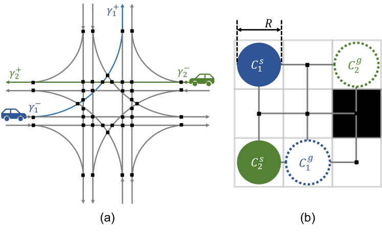
Figure 1: Illustration of the intersection model and the grid model we use. (a) Traffic intersection coordination model. (b) Grid map navigation model. Conflict points are marked as black dots. The black cells in (b) are static obstacles.

To tackle this challenge, some methods [7, 8, 9] discretize the action space and search using the motion primitives (i.e., elementary actions that an agent can perform) that satisfy the kinodynamic constraints. Those methods usually search in a high-dimensional state space to account for the kinodynamics of agents such as speed and acceleration. However, due to the discretization nature of those methods, the solutions generated by them do not fully capture the kinodynamic capacity of the agents and may be limited in expressiveness, leading to poor performance in some cases. In [1], a three-level method PBS-SIPP-LP (PSL) is introduced for intersection coordination problems, which is a special case for MAMP. PSL integrates search-based and optimization methods. Level 1 and Level 2 employ an extended MAPF planner to identify potential paths, which invokes Level 3 to optimize vehicle travel speeds through a Linear Programming (LP) model. However, PSL only considers the constraints on the speed of agents. Moreover, it makes a strong assumption that the agent moves through the intersection at a constant speed.

Taking inspiration from PSL, we introduce a three-level planner called PSB (PBS-SIPP-Bézier) to address the MAMP problem. Level 1 uses Priority-Based Search (PBS) [10] to resolve the collisions between agents. Level 2 employs an extended Safe Interval Path Planning (SIPP) [11] to search candidate paths for each agent given constraints from Level 1. Level 3 employs a Bézier curve-based [12] planner to seek feasible speed profiles for agents based on the constraints established in Level 2 while ensuring adherence to their kinodynamic limitations. In order to reduce the planning runtime, PSB utilizes a cache structure to store and reuse solutions from Level 3. Furthermore, PSB incorporates a duplicate detection and time window mechanism to speed up the planning process when extending PSB to the grid map navigation scenario.

The following content outlines our work in this paper: (1) We propose PSB, a MAMP planner capable of finding feasible trajectories for multiple agents and exploiting their complete kinodynamic capability. PSB can produce speed profiles with any degree of smoothness which is directly executable by the controller. To our knowledge, this is the first MAPF-based work in MAMP that incorporates the full kinodynamic capability for the extensive group of agents. (2) We show that PSB can efficiently handle the intersection coordination problem for autonomous vehicles with kinodynamic constraints (shown in Fig. 1(a)). Compared to the previously best algorithm PSL [1], PSB shows up to 49.79% improvement in terms of solution cost. (3) We extend PSB to a more general domain: mobile robots navigation in obstacle-rich grid maps (shown in Fig. 1(b)). PSB outperforms the previously best algorithm SIPP-IP [7], demonstrating an improvement of up to 27.12% in solution cost and increased scalability to handle up to 220 agents, as opposed to the limit of 80 agents in SIPP-IP, while maintaining a comparable runtime.

II Related Work

Multiple algorithms have been developed to tackle the challenges of kinodynamic constraints in MAMP problems. Traditional methods typically rely on control or optimization-based techniques to handle the MAMP in real-world robot scenarios. For instance, in [13], a vector field approach combined with model predictive control is used to find collision-free paths for multi-agent systems. Sun et al. [3] utilize a mixed-integer linear program to search timed waypoints that fulfill signal temporal logic constraints, which encapsulate the kinodynamic constraints. Alonso-Mora et al.[14] propose a series of optimization-based formulations customized for addressing local motion planning problems. These methods are proven to be effective in practical robot applications. However, they often encounter limitations in scalability, particularly when dealing with a large group of agents. For instance, the approach by [3] takes over 100 seconds to generate the solution for only a four-agent scenario.

Recently, MAPF methods have achieved significant progress in finding discrete collision-free paths for a large number of agents. These methods employ collision resolution techniques, such as Conflict-Based Search (CBS)[15, 5] and Prioritized-Based Search (PBS)[10], to effectively address collisions among agents while using single-agent solvers for individual agent path planning. Therefore, some methods take advantage of the MAPF methods to solve the MAMP problem.

One category of such methods uses discrete plans from the MAPF planner and smooths those plans to meet kinodynamic constraints. For instance, the method in [16] enforces agent adherence to their designated paths from the discrete MAPF plan. Then, it takes into account the speed constraints and employs an LP solver to generate an executable plan. Similarly, in [17], agent trajectories, represented as Bézier curves, are optimized by accounting for high-order kinodynamic constraints using the discrete plan from MAPF planners. These methods highly rely on the discrete initial plans from the MAPF planner, and their open-loop nature can lead to failures if no kinodynamically feasible trajectories can be derived from the initial plan.

Another category of methods discretizes the continuous action space into discrete motion primitives and uses them for state-space exploration. For instance, CBS-MP [8] integrates probabilistic roadmaps with CBS to handle agent collisions and employs motion-primitive-based search for individual planning. Cohen et al.[9] adapt CBS to continuous time and develop a bounded-suboptimal extension of SIPP for pathfinding for individual agents, where SIPP [11] is a variant of $A^{*}$ that can find optimal paths in dynamic environments. Moreover, Ali and Yakovlev [7] extend SIPP by incorporating a wait interval projection mechanism, which accounts for the time intervals during which an agent can wait. In [1], an extended variant of the PBS and SIPP method is harnessed for path exploration, accompanied by the integration of an LP solver to optimize the velocities of agents. However, these predefined discrete motion primitives are usually limited in expressiveness and might not capture the full possible actions that agents could exhibit.

III Problem Formulation

We define our MAMP problem by a graph $G=(V,E)$ and a set of $M$ agents $\mathcal{V}=\{a_{1},...,a_{M}\}$. The vertices of $G$, denoted as $c\in V$, are referred to as collision points which represent locations where collisions between agents may occur. Agents can move between collision points $c_{i}$ and $c_{j}$ along edge $e_{i,j}\in E$ while adhering to kinodynamic constraints, with the distance denoted as $d_{i}(c_{i},c_{j})\in\mathbb{R}^{+}$. The temporal-spatial profile, denoted as $\ell_{i}(t):\mathbb{R^{+}}\rightarrow\mathbb{R^{+}}$, characterizes the distance traveled by $a_{i}$ over time $t$ along a given path. The kinodynamic constraints limit the gradient of travel distance with respect to time up to $K$-th order:

$$\small\underline{U_{i}^{k}}<{d^{k}\ell_{i}(t)}/{dt^{k}}<\overline{U_{i}^{k}},\forall k\in{1,...,K}$$ (1)

where $\underline{U_{i}^{k}}$ and $\overline{U_{i}^{k}}$ are constant values that define the constraints on the $k$-th order gradient. Each agent initiates its movement from its specified start (collision point) $c_{i}^{s}$ with initial kinodynamic constraints as shown in Eq. 2 and moves toward its designated goal (collision point) $c_{i}^{g}$.

$$\small{d^{k}\ell_{i}(t)}/{dt^{k}}|_{t=0}=\underline{U_{i}^{k}},\forall k\in{1,...,K}$$ (2)

We define the path of $a_{i}$, if contains $m+1$ collision points, as $\phi_{i}=\{c_{i}^{0}=c_{i}^{s},c_{i}^{1},...,c_{i}^{m-1},c_{i}^{m}=c_{i}^{g}\}$ where $(c_{i}^{j-1},c_{i}^{j})\in E,j=1,\cdots,m$. The arrival time $T_{i}$ represents the time needed for $a_{i}$ to arrive at $c_{i}^{g}$. The combination of the path and the temporal-spatial profile is defined as trajectory. We denote $t_{i}(c_{i}^{j})$ as the time when $a_{i}$ reaches the collision point $c_{i}^{j}$, and $\tau_{i}(c_{i}^{j})$ represents the duration that it occupies $c_{i}^{j}$. Therefore, $a_{i}$ departs from $c_{i}^{j}$ at time $t_{i}(c_{i}^{j})+\tau_{i}(c_{i}^{j})$. In the event that both $a_{i}$ and $a_{j}$ pass through the same collision point c, a collision occurs iff the time intervals $[t_{i}(c),t_{i}(c)+\tau_{i}(c))$ and $[t_{j}(c),t_{j}(c)+\tau_{j}(c))$ overlap.

III-1 Intersection Model

For the intersection coordination problem, we adopt the model from [18]. As shown in Fig. 1 (a), the intersection has a set of entry lanes $\Gamma^{-}$ and a set of exit lanes $\Gamma^{+}$. Each agent $a_{i}\in\mathcal{V}$, with a length of $L_{i}$, has a traveling request from the entry lane $c_{i}^{0}=\gamma_{i}^{-}\in\Gamma^{-}$ to the exit lane $c_{i}^{m}=\gamma_{i}^{+}\in\Gamma^{+}$ with the earliest start time $e_{i}\in\mathbb{R}^{+}$ (i.e. the earliest time the agent i can reach at the entry lane). To prevent agents from making sharp turns, they are constrained to follow the predefined path (gray lines in Fig. 1 (a)). We assume the agents can wait before the entry lane without any collision. After entering the intersection, the minimum speed of agents is strictly positive. If both $a_{i}$ and $a_{j}$ start from the same entry lane with $e_{i}<e_{j}$, then a overtake happens if $\exists k,h$ that $t_{i}(c_{i}^{k})\geq t_{j}(c_{j}^{h})$ where $c_{i}^{k}=c_{j}^{h}$. Our task is to generate trajectories for all agents so that no collisions or overtakes happen while minimizing the sum of their arrival time.

III-2 Grid Model

In contrast to the intersection model, the grid map navigation model involves an extra spatial domain search, leading to increased complexity and exponential growth of the search space. In this model, we adopt a four-neighbor grid map representation as shown in Fig. 1 (b). Notably, the agents are able to stop at any location, which imposes a minimum speed constraint of $\underline{U_{i}^{1}}=0$. We assume that the agent has a radius of R. All the agents start simultaneously and remain at their respective goals once they reach them. Our primary objective is to plan collision-free trajectories for all the agents, aiming to minimize the sum of their travel time.

IV MAMP on Intersection

This section begins with a system overview of our proposed algorithm PSB, followed by a discussion of the specifics of our trajectory optimization formulation and method. After that, we delve into the techniques used to tackle runtime challenges.

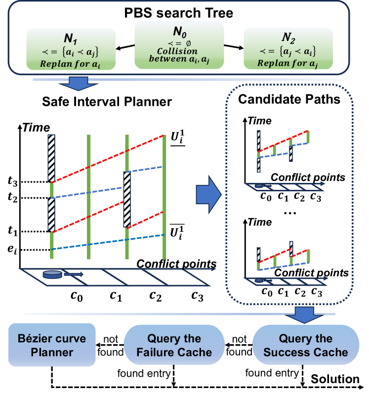
Figure 2: Overview of PSB. The green segments represent the safe time intervals while the shadowed strips represent the time intervals occupied by other agents.

IV-A System Overview

PSB consists of a three-level planner as illustrated in Fig.2, with Level 1 and Level 2 extended from PSL[1]. Level 1 uses PBS to resolve collisions among agents through priority ordering searching, where the trajectory of each agent is planned by Level 2. Given the priority ordering from Level 1, Level 2 uses an extended SIPP to search for the optimal trajectory for an agent, where the temporal-spatial profile of the trajectory is optimized by Level 3. Given the path (together with some temporal constraints) from Level 2, Level 3 uses BCP (Bézier-Curve-based Planner) to generate the optimal temporal-spatial profile.

IV-A1 PBS-based planner

We adopt PBS [10] to resolve collisions among agents. If two agents have a priority ordering, the trajectory of the agent with lower priority must avoid collisions with the trajectory of the agent with higher priority. The goal is to find a set of priority orderings for agents so that they do not collide with each other. To achieve this, we search a binary Priority Tree (PT) in a depth-first manner. Each PT node contains a set of priority orderings and a set of trajectories consistent with the priority orderings. We initialize the root PT node by sorting the priority orderings of agents starting from the same entry lane based on their earliest start time to prevent overtake. Then, Level 2 is called to plan trajectories for agents at each lane from the highest priority to the lowest priority. We expand PT nodes by searching for collisions between agents and generating child PT nodes with additional priority orderings to address the collisions. As shown in Fig. 2, if a collision between agents $a_{i}$ and $a_{j}$ is detected in node $N_{0}$, the algorithm resolves this collision by expanding $N_{0}$ into two child nodes $N_{1}$ and $N_{2}$. In $N_{1}$, $a_{i}$ is given higher priority than $a_{j}$, while in $N_{2}$, $a_{j}$ is given higher priority than $a_{i}$. Then, in each child node, we use Level 2 to plan trajectories for each agent based on the priority orderings in that node. The algorithm terminates and returns the trajectories when a PT node with collision-free trajectories for all agents is found. On the contrary, if no such PT node is found, the algorithm returns no solution.

IV-A2 Safe Interval Planner

The objective for Level 2 is finding a trajectory that has the minimum arrival time for single agent $a_{i}$ without colliding with higher-priority agents. To achieve this, we first use a modified SIPP to search paths with corresponding safe interval sequences and then use Level 3 to specify the temporal-spatial profile considering kinodynamic constraints. Here, safe interval sequence, denoted as $S_{i}=\{[lb_{i}^{0},ub_{i}^{0}),...,[lb_{i}^{m},ub_{i}^{m})\}$, is the time intervals along the path of $a_{i}$ that guarantee no collision with higher-priority agents, where $lb_{i}^{k}$ and $ub_{i}^{k}$ are the earliest and latest time $a_{i}$ can stay at collision point $c_{i}^{k}$. We provide an illustrative example of the search process in Fig. 2. The comprehensive illustration of Level 2 can be found in [1]. While we use a 1-D example for demonstration, as later shown in the grid model, this search process can be done in high-dimensional space. We begin by constructing a safe interval table, which associates each collision point with a set of safe intervals, based on the priority orderings from Level 1. As shown in Fig. 2, assume that there are two safe intervals: $[e_{i},t_{1})$ and $[t_{2},t_{3})$ at collision point $c_{0}$. We generate two SIPP nodes based on these intervals and insert them into the open list. During each iteration, we select the node with the smallest $f$-value (i.e., the sum of the lower bound of its safe interval and the minimum travel time required to reach the goal from the location of the node). In this example, we choose the node with safe interval $[e_{i},t_{1})$. During node expansion, in order to speed up the search process while guaranteeing completeness, Level 2 uses relaxed kinodynamic constraints. Specifically, we assume that $a_{i}$ occupies each collision point only an instant of time while having the flexibility to adjust its speed within the range $[\underline{U_{i}^{1}},\overline{U_{i}^{1}}]$ instantaneously. In our case, as the agent moves from $c_{i}^{0}$ to $c_{i}^{1}$, a new time interval is generated at $c_{i}^{1}$ as $[e_{i}+t_{min},t_{1}+t_{max})$, where $t_{min}=d_{i}({c_{0}},{c_{1}})/\overline{U_{i}^{1}}$ and $t_{max}=d_{i}({c_{0}},{c_{1}})/\underline{U_{i}^{1}}$ represent the minimum and maximum time required for the agent to reach $c_{i}^{1}$ from $c_{i}^{0}$. We iterate the safe intervals at $c_{1}$ within $[e_{i}+t_{min},t_{1}+t_{max})$ and insert them into the open list. When a node reaches the goal, we backtrack to retrieve the complete path and its associated safe interval sequence $S_{i}^{q}$. Then, we call Level 3 to determine the kinodynamically feasible trajectory. If Level 3 succeeds and the newly found trajectory has a smaller arrival time, we update the current best trajectory. We terminate the search and return the current best trajectory if no node in the open list has a lower $f$-value than the arrival time of the current best trajectory. As shown in [1], Level 2 guarantees to return the optimal trajectory when Level 3 is optimal and complete.

IV-A3 Bézier Curve Planner

The goal of Level 3 is to generate a kinodynamically feasible temporal-spatial profile $\ell_{i}(t)$ within safe interval sequence while minimizing the arrival time. In BCP, we use Bézier curve $B^{T_{i}}(t)$, where $T_{i}$ is the arrival time, to represent $\ell_{i}(t)$. Thus, this problem can be reformulated as minimizing the arrival time $T_{i}$ and finding control points $P_{i}$ for $B^{T_{i}}(t)$ that satisfies the kinodynamic and collision-free constraints. As demonstrated in Sec. IV-C, Level 3 is complete and optimal.

IV-B Background on Bézier Curves

Bézier curve [12], denoted as $B(t)$, is able to approximate any continuous function within the interval $[0,1]$ with a sufficiently large number of control points. This property makes it an ideal choice for modeling $\ell(t)$ [17]. In order to represent the real-world trajectory, $t$ should be defined on $[0,T]$. Thus, we scale the Bernstein basis polynomials by the factor of $T$:

$$\small\begin{array}[]{cl}&B_{r,n}^{T}(t)=\binom{n}{r}(\frac{t}{T})^{r}(\frac{T-t}{T})^{n-r},\;r\in\{0,1...,n\}\\ &B^{T}(t)=\sum_{r=0}^{n}p_{r}B_{r,n}^{T}(t),\;t\in[0,T]\\ \end{array}$$ (3)

where $P=\{p_{0},...,p_{n}\}$ are ${n+1}$ control points.

As proven in [12], the Bézier curve has properties that can help solve the kinodynamically feasible trajectory efficiently. Specifically, $B^{T}(t)$ is bounded by the convex hull of its control points P for $t\in[0,T]$. Moreover, the curve always starts at the first control point and ends at the last control point (i.e., $B^{T}(0)=p_{0},\;B^{T}(T)=p_{n}$). At the same time, the derivative of the $n$-degree scaled Bernstein polynomial is another scaled Bernstein polynomial with degree $n-1$:

$$\small\begin{array}[]{cl}&\frac{d^{k}B^{T}(t)}{dt^{k}}=\sum_{r=0}^{n-k}{p^{k}_{r}}B_{r,n-k}^{T}(t),\;t\in[0,T]\\ &{p^{k}_{r}}=\frac{n!}{(n-k)!T^{k}}\sum_{j=0}^{k}(-1)^{j}\binom{k}{j}p_{n-j},\forall r\in\{0,...,n-k\}\end{array}$$ (6)

Here, $P^{k}=\{p^{k}_{0},...,p^{k}_{n-k}\}$ are the control points for the $k$-th gradient of $B^{T}(t)$. With the convexity property and the gradient property of the Bézier curve, we can translate the kinodynamic constraints discussed in Eq. 1 to the constraints of the control points: $\underline{U_{i}^{k}}\leq{p^{k}_{r}}\leq\overline{U_{i}^{k}},\;\forall r\in\{0,1...,n-k\}$.

IV-C Bézier Curve based path planner

As discussed in IV-A, BCP aims at finding a temporal-spatial profile, represented by $B^{T_{i}}(t)$, within the safe interval sequence $S_{i}^{q}$ given by Level 2 while minimizing the arrival time. In this section, we introduce the process of computing control points for a specified arrival time, followed by a discussion of the method to determine the optimal arrival time.

IV-C1 Find Bézier curve given arrival time

Given arrival time $T_{i}$, our objective is to determine control points for $B^{T_{i}}(t)$ that meet all constraints. We formulate this task as an LP problem:

$$\small\min\; \delta$$ (7)

$$s.t.\; \delta\geq 0$$ (8)

$$p_{0}=d_{i}^{0},\quad p_{n}=d_{i}^{m},\quad p_{0}^{k}=\underline{U_{i}^{k}},\;\forall k\in 1,...,K$$ (9)

$$B^{T_{i}}(lb_{i}^{j})<d_{i}^{j}+\delta,\;\forall j\in 1,...,m$$ (10)

$$B^{T_{i}}(ub_{i}^{j}-L_{i}/\omega)>d_{i}^{j}+L_{i}-\delta,\;\forall j\in 1,...,m$$ (11)

$$\underline{U_{i}^{k}}-\delta\leq{p^{k}_{r}}\leq\overline{U_{i}^{k}}+\delta,$$ (12)

$$\hfill\quad\quad\quad\quad\forall k\in 1,...,K,\quad\forall r\in 0,1,...,n-k$$

where $d_{i}^{j}=\sum_{r=1}^{r=j}d_{i}(c_{r-1},c_{r})$. Agents initiate from the entry lane with initial kinodynamic constraints and terminate at the exit lane. [Eq. 9] Obtained from Level 2, a path along with safe interval sequence $S_{i}^{q}={[lb_{i}^{0},ub_{i}^{0}),...,[lb_{i}^{m},ub_{i}^{m})}$ is available. Our goal is to have the agent visit each collision point within the safe interval along the path. Given the challenge of finding a closed-form inverse function for $d_{i}^{j}=B^{T_{i}}(t)$, we instead prohibit the agent from arriving before $lb_{i}^{j}$ or leaving after $ub_{i}^{j}$ at the collision point. [Eq. 10-11] Here, $\omega$ is a constant derived from wave speed [19] (we set it to 7 in our experiment). The kinodynamic constraints can be translated to the constraints on the control points using properties shown in Sec. IV-C. [Eq. 12] We introduce a slack variable $\delta$ to relax those constraints. As shown in Fig. 3, if valid $B^{T_{i}}$ exists for a specific $T_{i}$, the optimal value $\delta^{*}$ derived from Eq. 7 is zero.

IV-C2 Search for optimal arrival time

To determine the shortest arrival time $T^{*}$, BCP employs a binary search method, extended from the method used in [17]. Leveraging the Single Interval Theorem discussed in [17], we can assume there exists a maximum feasible arrival time range $[T_{min},T_{max}]$, where $\forall T\in[T_{min},T_{max}]$, $\delta^{*}=0$ for Eq. 7, $\forall T\notin[T_{min},T_{max}],\delta^{*}>0$. Therefore, the optimal arrival time $T^{*}$ equals to $T_{min}$. During the binary search, we initially establish lower bound $T_{lb}$ and upper bound $T_{ub}$ for $T^{*}$. Then we apply Theorem 3 from [17], which asserts that $\delta^{*}$ monotonically decreases in the interval $[0,T_{min})$ and monotonically increases in the interval $(T_{max},\infty)$, to find the search direction. By calculating the gradient of $\delta^{*}$ at $(T_{lb}+T_{ub})/2$, we can determine which half of the range should be further explored.

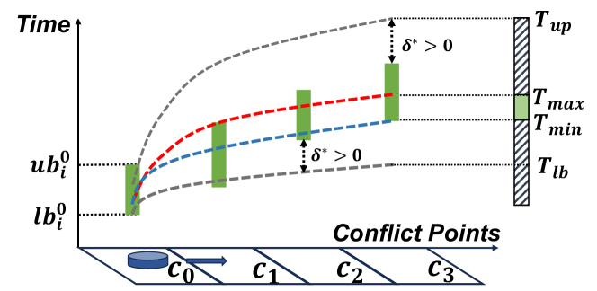
Figure 3: Illustration of BCP. The agent moves along the x-axis. The green segments are the safe intervals.

IV-C3 Pseudocode for BCP

As shown in Algorithm 1, we take the safe interval sequence $S_{i}^{q}$ as input. We initialize the lower bound $T_{lb}$ for $T^{*}$ using the earliest arrival time $lb_{i}^{m}$ at $c_{i}^{g}$. [Line 2] Then, we check if the latest arrival time $ub_{i}^{m}$ at $c_{i}^{g}$ exists. In case where $ub_{i}^{m}$ is finite, the upper bound $T_{ub}$ for $T^{*}$ is initialized using $ub_{i}^{m}$. [Line 3] Conversely, if $ub_{i}^{m}=\infty$, from Lemma 1, $T_{ub}$ can be determined using Eq. 13.

$$\small\begin{array}[]{ll}\min_{t}&\quad t+(d_{i}^{m}+L_{i})/{\underline{U_{i}}}\\ s.t.&\quad lb_{j}\leq t+d_{i}^{j}/\underline{U_{i}},\quad\forall j\in\{1,...,m\}\end{array}$$ (13)

Then, we determine if there is feasible $T_{i}$ in $[T_{lb},T_{ub})$ according to Lemma 2. As shown in function IsSolutionExist, we first compute the gradient of $\delta^{*}$ at $T_{lb}$ and $T_{ub}$. If no solution exists, BCP returns no solution. [Line 6-7] Otherwise, we proceed with the binary search to find $T^{*}$ within the range $[T_{lb},T_{ub})$, and this search continues until the range $[T_{lb},T_{ub})$ is smaller than a predefined threshold $\epsilon_{2}$ (We use $\epsilon_{2}=0.1$ in our experiments). [Line 8] In each iteration, we average $T_{lb}$ and $T_{ub}$ to get $T_{mid}$ and solve Eq. 7 at $T_{mid}$. [Line 9-10] If $slack(T_{mid})=0$, it indicates that $T_{mid}\in[T_{min},T_{max})$. Consequently, we use $T_{mid}$ as the new upper bound for $T^{*}$. [Line 11] On the other hand, if $slack(T_{mid})\neq 0$, we calculate the gradient of $\delta^{*}$ at $T_{mid}$. If $\nabla\delta^{(}T_{mid})>0$, it implies that $T_{mid}>T_{max}$, and we can use $T_{mid}$ as the new $T_{ub}$. [Line 13-14] Conversely, it can be concluded that $T_{mid}<T_{min}$, and we can use $T_{mid}$ as the new $T_{lb}$. [Line 15]

Lemma 1.

If the latest arrival time at the exit lane is unbounded, $ub_{i}^{m}=\infty$, the optimal objective value for Eq. 13 always exists and resides within the interval $[T_{min},T_{max}]$.

Proof.

If the minimum speed of agents is strictly positive, any time interval with a finite upper bound restricts subsequent time intervals along the path to a finite value. If $ub_{i}^{m}$=$\infty$, it means that the upper bound for all safe intervals in $S_{i}^{q}$ is infinite. In such a case, a valid solution always exists wherein the agent waits at the entry lane and maintains a continuous movement at $\underline{U_{i}}$ throughout the intersection. ∎

Lemma 2.

If $\exists\ \hat{T}\in[T_{lb},T_{ub}]$, such that $\delta^{*}=0$ for Eq. 7 given $\hat{T}$, then $\nabla\delta_{T_{lb}}\leq 0$ and $\nabla\delta_{T_{ub}}\geq 0$.

Proof.

From the definition, we can have that $[T_{min},T_{max}]\neq\emptyset$. As $\delta^{*}$ is monotonically decrease at $[0,T_{min}]$ and monotonically increase at $[T_{max},\infty]$. By applying $T_{lb}\leq T_{min}$ and $T_{min}\leq T_{ub}$, we can have $\nabla\delta_{T_{lb}}\leq 0$ and $\nabla\delta_{T_{ub}}\geq 0$. ∎

Lemma 3.

For infinite control points, BCP guarantees to find the optimal arrival time $T^{*}$ and corresponding control points $P^{*}$ if one exists and returns failure otherwise.

Proof.

With infinite control points, the Bézier curve is able to approximate any continuous function in $[0,T]$. Thus, we can always find $P^{*}$ given $T^{*}$, if a feasible temporal-spatial profile exists. At the same time, with Lemma 1, the upper bound for $T_{i}$ always exists. As shown in Theorem 3 of [17], the binary search in BCP can find the $\epsilon_{2}$-close optimal $T_{i}^{*}$. ∎

Theorem 1.

(Completeness and Suboptimality of PSL). PSB is complete and finds a sub-optimal solution.

Proof.

We adopt Level 1 and Level 2 from [1], where Level 2 is proven to be complete and optimal, while Level 1 is complete and suboptimal. For Level 3, we apply Lemma 3 to prove it is complete and representation-optimal. Therefore, our proposed PSB is both complete and suboptimal. ∎

Algorithm 1 Pseudocode for Bézier path optimization

Input: Path of agent and safe interval sequence $S_{i}^{q}$
      Output: The $\epsilon-optimal\;T^{*}$ and control points $P^{*}$
      Let $\Delta$ be a sufficient small positive number
      Function IsSolutionExist $(T_{lb},T_{ub})$
           $\nabla\delta_{T_{lb}}={(slack(T_{lb}+\Delta)-slack(T_{lb}))}/{\Delta}$
           $\nabla\delta_{T_{ub}}={(slack(T_{ub}+\Delta)-slack(T_{ub}))}/{\Delta}$
           return $\nabla\delta_{T_{lb}}\leq 0\;and\;\nabla\delta_{T_{ub}}\geq 0$

1:Let $slack(T)$ denote the value of $\delta$ from Eq. 7

2:Initialize $T_{lb}\leftarrow lb_{m}$, $T^{*}\leftarrow null$

3:if $ub_{m}\neq\infty$ then  Initialize $T_{ub}\leftarrow ub_{m}$

4:else

5:     Initialize $T_{ub}\leftarrow$ UpperBoundSolver using Eq. 13

6:if ${!IsSolutionExist}(T_{lb},T_{ub})$ then

7:     return $no\;solution$

8:while $T_{ub}-T_{lb}>\epsilon$ do

9:     $T_{mid}\leftarrow(T_{lb}+T_{ub})/2$

10:     if $slack(T_{mid})=0$ then

11:         $T_{ub}\leftarrow T_{mid}$, $T^{*}\leftarrow T_{mid}$

12:     else

13:         if ${(slack(T_{mid}+\Delta)-slack(T_{mid}))}/{\Delta}>0$ then

14:              $T_{ub}\leftarrow T_{mid}$

15:         else$\quad T_{lb}\leftarrow T_{mid}$               

16:if $T^{*}=null$ then  return $no\;solution$

17:else return $T^{*}$ and $P^{*}$

IV-D Cache for Safe Interval Planner

As BCP encounters recurrent LP solving, calling BCP frequently can lead to a significant increase in runtime. To address this issue, we implement two types of caches, namely SuccessCache and FailureCache. These caches utilize the results of previous BCP calls to expedite the search process. SuccessCache is designed to retain safe interval sequences for which BCP successfully finds a feasible temporal-spatial profile. Each entry in SuccessCache includes a path with an associated safe interval sequence and a temporal-spatial profile. During the search process, if a path matches the path of an entry from SuccessCache and their associated safe interval sequences are identical, we can directly reuse the temporal-spatial profile from that entry. We define two paths $\phi_{i}$ and $\phi_{j}$ matches iff they contain the same number of collision points and the travel distance to corresponding collision points is the same, i.e., $d_{i}(c_{i}^{k-1},c_{i}^{k})=d_{j}(c_{j}^{k-1},c_{j}^{k}),\forall k\in 1,...,m$. In contrast, FailureCache stores safe interval sequences that BCP is unable to find a temporal-spatial profile satisfying both collision-free and kinodynamic constraints. This cache helps avoid redundant attempts for safe interval sequences that have been previously proven to have no feasible solution. As discussed in Lemma 4, if a safe interval sequence $S_{i}^{q}$ is contained by a safe interval sequence $S_{f}$ stored in FailureCache, we can infer that BCP can not found a temporal-spatial profile for $S_{i}^{q}$. A Safe interval sequence $S_{1}=\{[lb_{i}^{0},ub_{i}^{0}),...,$ $[lb_{i}^{m},ub_{i}^{m})\}$ contains safe interval sequence $S_{2}=\{[lb_{k}^{0},$ $ub_{k}^{0}),...,[lb_{k}^{m},ub_{k}^{m})\}$, iff the associated paths of $S_{1}$ and $S_{2}$ matches, and $\forall j\in\{0,...,m\},lb_{i}^{j}\leq lb_{k}^{j},ub_{i}^{j}\geq ub_{k}^{j}$.

Lemma 4.

If BCP cannot find a feasible temporal-spatial profile for safe interval sequence $S_{f}$, and $S_{f}$ contains $S_{i}^{q}$, then there will be no feasible temporal-spatial profile for $S_{i}^{q}$.

Proof.

If a temporal-spatial profile $B^{T_{q}}(t)$ for $S_{i}^{q}$ exists, this profile can also be the solution for $S_{f}$. ∎

As shown in Fig. 2, during the search process of Level 2, after obtaining safe interval sequence $S_{i}^{q}$ through backtracking, we first check SuccessCache. If an entry is found in the cache, we return the stored temporal-spatial profile as the solution for $S_{i}^{q}$. However, if no entry is found in SuccessCache, we continue to check FailureCache. If an entry is found in FailureCache that contains $S_{i}^{q}$, we directly disregard $S_{i}^{q}$ as unsolvable. Otherwise, BCP is called to find a feasible temporal-spatial profile for $S_{i}^{q}$. If BCP returns a valid profile, $S_{i}^{q}$ along with the obtained profile, is stored in SuccessCache. Otherwise, $S_{i}^{q}$ is inserted into FailureCache.

V MAMP on Grid Model

In the intersection model, agent paths are fixed given the entry and exit lanes, allowing us to focus solely on searching for safe time intervals in the time domain. However, in the grid model, we must also consider the path and conduct spatial domain searches. In this section, we extend PSB to address the MAMP problem on the grid model. Level 1 can be directly applied to the grid model. In Level 2, we introduce a duplicate detection mechanism to prevent the expansion of redundant nodes. For Level 3, given Lemma 1 relies on the assumption of positive minimum speed, we incorporate an exponential increase method to initialize the upper bound. To address the complexities of this scenario, we introduce a time window mechanism to expedite the planning process.

V-1 Upper bound estimation for arrival time

In the grid model, agents are allowed to stop at any location. Therefore, when the upper bound for the safe interval at $c_{i}^{g}$ is unbounded ($ub_{i}^{m}=\infty$), using Eq. 13 to initialize $T_{ub}$ is not applicable. Hence, we employ an exponential increment approach to establish the initial value for $T_{ub}$. We begin by initializing $T_{ub}$ using $T_{lb}$ and then employ a loop to search for an appropriate $T_{ub}$. During each iteration, we double $T_{ub}$ and evaluate the gradient of $\delta^{*}$ at $T_{ub}$. If the gradient is non-negative, it indicates that $T^{*}$ is confined to the interval $[T_{lb},T_{ub}]$. We conclude the search process and adopt the current $T_{ub}$ as the initialization. However, if $T_{ub}$ reaches infinity, represented by the large value of $4000$ in our experiment, the algorithm returns no solution. The subsequent steps mirror the Sec. IV-C, enabling the determination of the optimal arrival time and control points within the range of $[T_{lb},T_{ub}]$.

V-2 Duplicate detection

Since the input of Level 3 contains information not only from the goal node but also from its ancestor nodes, the dominance check in SIPP is not applicable during our search. Instead, we always add generated nodes to the open list even if nodes with identical locations and intervals have been previously added. However, directly applying Level 2 to the grid map navigation problem causes an exponential rise in the number of expanded nodes. This growth is primarily attributed to the presence of redundant nodes, denoted as symmetry nodes. We define two nodes as symmetrical if they have the same location and all their ancestor nodes share identical time intervals. For example, in Fig. 1, if we only consider the movement of agent 1, expanding the SIPP node at A generates two nodes at B and C. Expanding these nodes further results in two symmetrical nodes at D. In the context of BCP, these identical intervals correspond to the same temporal-spatial profile. Additionally, since those nodes have the same location, any nodes expanded from them inherently possess the same time intervals and locations. Thus, we only need to retain one of the nodes without losing completeness. During node expansion, we ignore newly expanded nodes that have a symmetry node in the open list.

V-3 Windowed PSB

To handle scenarios with long planning horizons, we use a time window with replanning strategy [20, 21]. In each replanning iteration, we only focus on the collisions with higher-priority agents that occur within the current time window (with size $t_{W}$). Once collision-free trajectories are determined within the time window, we shift the window by a predetermined replan interval $t_{s}<t_{W}$. (In our experiment, we set $t_{s}=4,t_{W}=6$.) By recurrently replanning, we can progressively advance the time window and compute the full trajectories for all agents.

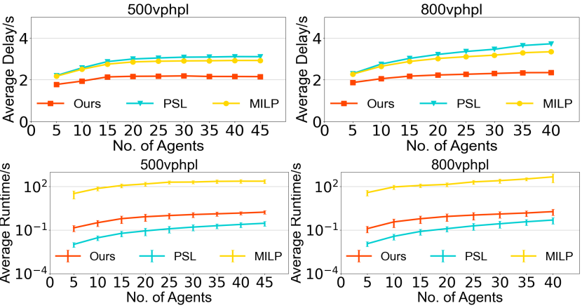
Figure 4: Average delay and average runtime for intersection model. Runtime in log scales. The error bars show the standard deviations.

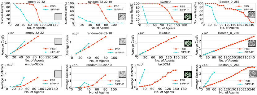
Figure 5: The success rate, solution cost, and runtime of both PSB and SIPP-IP across all maps. The solution cost and runtime values are averaged only for scenarios where the planner successfully generates a solution.

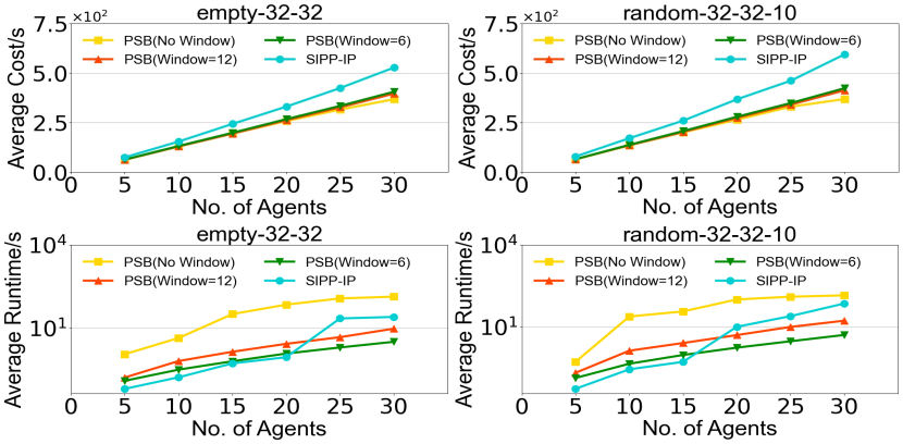
Figure 6: Runtime and cost for PSB with various window sizes.

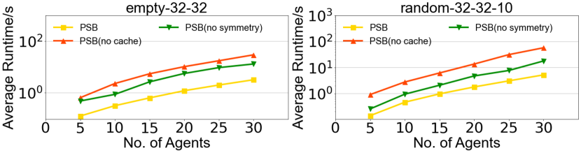
Figure 7: Average runtime for ablation study.

VI Empirical Evaluation

Both PSB and baseline methods are implemented in C++ and utilize CPLEX to solve the programming models. We conducted all experiments on an Ubuntu 20.04 machine equipped with an AMD 3990x processor and 188 GB of memory. Our codes were executed on a single core for all computations.

VI-A MAMP on Intersection

VI-A1 Baseline Algorithms

For our comparison, we include two baseline methods. The first baseline is the method proposed in [18], which utilizes a MILP formulation to obtain the optimal trajectories for the agents. The second baseline is PSL [1], which solves the intersection coordination as a MAPF problem. It is important to note that both methods assume that the agent travels across the intersection at a constant speed.

VI-A2 Simulation Setup

In our experiments, we utilize a simulation setup identical to the one discussed in [18]. As depicted in Fig. 1, the lane width is $3.66\;m$, the right-turn radius is 1.83m, and the left-turn radius is $9.14\;m$. The length of each agent is $5\;m$. In this setup, the probability of an agent going straight is 80%, while the probability of it turning left or right is 20%. For simplicity, we only considered the speed and acceleration constraints. We set a minimum speed of $3\;m/s$ for all agents. For agents that turn left, the maximum speed is limited to $5\;m/s$, while other agents have their maximum speed restricted to $15\;m/s$. Additionally, the acceleration of agents ranges from $[-2,5]\;m/{s^{2}}$. To assess the performance of our method, we randomly sample travel requests from two different demands: 500 vphpl (i.e., 500 vehicles per hour per lane) and 800 vphpl. The results of the experiment are averaged over 25 instances from each demand level.

VI-A3 Comparison

In our problem formulation, the objective is to minimize the sum of the arrival time for all agents. However, the arrival time of the agents depends on their earliest start time. Thus, we instead compare the average delay, which is a popular metric used in transportation. This metric measures the average difference between the arrival time and the earliest arrival time (i.e., the earliest time an agent can reach its goal, defined by $e_{i}+d_{i}(c_{i}^{s},c_{i}^{g})/\overline{U_{i}^{1}}$) among agents. As shown in Fig. 4, while PSB shows a relatively longer runtime compared to PSL, PSB shows an improvement of up to 41.15% for 500 vphpl demands and 49.79% for 800 vphpl demands compared to PSL in terms of average delay. Although MILP is optimal under constant speed assumption[18], it still produces worse solutions than ours. In terms of runtime, MILP is significantly slower than both PSL and PSB. At the same time, the difference between the solution quality of PSL and MILP is much smaller than the difference between PSB and PSL. These improvements arise from the fact that the baseline methods assume the constant speed during intersection traversal, while our planner considers the full kinodynamic capabilities of agents. We also noticed that, in the 500 vphpl scenario, the average delay curves for all three methods level off as the number of agents increases. In contrast, in the 800 vphpl scenario, only the delay curve for PSB levels off, suggesting that our method can find a stable solution for higher demand scenarios.

VI-B MAMP on Grid Model

VI-B1 Baseline Algorithms

In this experiment, we compare our method with a straightforward extension of SIPP-IP[7]. SIPP-IP is a state-of-the-art planner designed to accommodate kinodynamic constraints, making it a suitable representation of motion-primitive-based methods. The same kinodynamic motion primitives as [7] are used during the evaluation. To adapt SIPP-IP for multi-agent scenarios, we replaced Level 2 and Level 3 in PSB with the SIPP-IP.

VI-B2 Simulation Setup

We evaluated PSB and SIPP-IP using the four-neighbor grid maps from the MovingAI benchmark [22]. The maps used for evaluation were empty (size: 32$\times$32), random (size: 32$\times$32), lak303d (size: 194$\times$194), and Boston (size: 256$\times$256). For each map, we conducted experiments with a progressive increment in the number of agents, using an average of 25 random instances from the benchmark set. The agents were modeled as disks with a diameter of $0.99\;cell$. All agents followed identical kinodynamic constraints, which, similar to the intersection model, encompassed only speed and acceleration constraints. The speed is bounded by the range of $[0,2]\;cell/s$, while the acceleration is confined to $[-0.5,0.5]\;cell/s^{2}$.

VI-B3 Comparison

We evaluate solution quality using the sum of the travel time of all agents. As shown in Fig. 5, the solution quality of PSB is better than that of the baseline method. At the same time, PSB achieves comparable or better runtime performance compared to the baseline method. PSB also outperforms the baseline method across all four environments in terms of success rate, which represents the ratio of instances solved within $300s$ over all instances. This can be attributed to two factors. Firstly, the longer runtime of SIPP-IP in scenarios with more agents makes it easier to hit the preset cutoff time. Secondly, the solution from SIPP-IP is limited in expressiveness, leading to failures in solving certain cases. For instance, when $c_{i}^{g}$ is adjacent to the $c_{i}^{s}$, SIPP-IP encounters difficulties in finding an appropriate solution (The accelerating primitive defined in [7] takes 4 cells).

VI-B4 Ablation study

We first evaluate the influence of window size $t_{W}$ by comparing our method under different window sizes: $t_{W}$=$6$, $t_{W}$=$12$, and $t_{W}$=$\infty$. As shown in Fig. 6, we observe marginal improvement in solution quality as we increase the value of $t_{W}$(less than 5% from $t_{W}$=$6$ to $t_{W}$=$\infty$), while causing a significant rise in runtime. Furthermore, as shown in Fig 7, PSB exhibits a runtime improvement of up to 88.58% compared to PSB without the cache mechanism and 76.71% improvement over PSB without the symmetry elimination mechanism. Importantly, these two mechanisms do not affect the solution quality of the algorithms.

VII Conclusion

This paper introduces PSB, a three-level multi-agent motion planner designed to tackle the MAMP problem with real-world kinodynamic constraints. Our method is able to produce smooth and executable solutions utilizing the full kinodynamic capacity of agents, addressing a limitation often faced by existing methods. We apply PSB to two domains: traffic intersection coordination for autonomous vehicles and obstacle-rich grid map navigation for mobile robots. In both domains, PSB outperforms the baseline methods with up to 49.79% improvement in terms of solution quality. At the same time, our method achieves comparable performance in runtime.

References

- [1] J. Li, T. A. Hoang, E. Lin, H. L. Vu, and S. Koenig, “Intersection coordination with priority-based search for autonomous vehicles,” in Proceedings of the AAAI Conference on Artificial Intelligence, vol. 37, 2023, pp. 11 578–11 585.
- [2] W. Hönig, S. Kiesel, A. Tinka, J. W. Durham, and N. Ayanian, “Persistent and robust execution of MAPF schedules in warehouses,” IEEE Robotics and Automation Letters, vol. 4, no. 2, pp. 1125–1131, 2019.
- [3] D. Sun, J. Chen, S. Mitra, and C. Fan, “Multi-agent motion planning from signal temporal logic specifications,” IEEE Robotics and Automation Letters, vol. 7, no. 2, pp. 3451–3458, 2022.
- [4] R. Stern, N. Sturtevant, A. Felner, S. Koenig, H. Ma, T. Walker, J. Li, D. Atzmon, L. Cohen, T. Kumar et al., “Multi-agent pathfinding: Definitions, variants, and benchmarks,” in Proceedings of the International Symposium on Combinatorial Search, vol. 10, no. 1, 2019, pp. 151–158.
- [5] J. Li, W. Ruml, and S. Koenig, “EECBS: A bounded-suboptimal search for multi-agent path finding,” in Proceedings of the AAAI Conference on Artificial Intelligence, vol. 35, no. 14, 2021, pp. 12 353–12 362.
- [6] J. Li, D. Harabor, P. J. Stuckey, H. Ma, G. Gange, and S. Koenig, “Pairwise symmetry reasoning for multi-agent path finding search,” Artificial Intelligence, vol. 301, p. 103574, 2021.
- [7] Z. A. Ali and K. Yakovlev, “Safe interval path planning with kinodynamic constraints,” in Proceedings of the AAAI Conference on Artificial Intelligence, vol. 37, 2023, pp. 12 330–12 337.
- [8] I. Solis, J. Motes, R. Sandström, and N. M. Amato, “Representation-optimal multi-robot motion planning using conflict-based search,” IEEE Robotics and Automation Letters, vol. 6, no. 3, pp. 4608–4615, 2021.
- [9] L. Cohen, T. Uras, T. Kumar, and S. Koenig, “Optimal and bounded-suboptimal multi-agent motion planning,” in Proceedings of the International Symposium on Combinatorial Search, vol. 10, 2019, pp. 44–51.
- [10] H. Ma, D. Harabor, P. J. Stuckey, J. Li, and S. Koenig, “Searching with consistent prioritization for multi-agent path finding,” in Proceedings of the AAAI conference on artificial intelligence, vol. 33, 2019, pp. 7643–7650.
- [11] M. Phillips and M. Likhachev, “Sipp: Safe interval path planning for dynamic environments,” in Proceedings of the IEEE International Conference on Robotics and Automation, 2011, pp. 5628–5635.
- [12] G. G. Lorentz, Bernstein polynomials. American Mathematical Society, 2012.
- [13] R. Hegde and D. Panagou, “Multi-agent motion planning and coordination in polygonal environments using vector fields and model predictive control,” in Proceedings of the IEEE European Control Conference, 2016, pp. 1856–1861.
- [14] J. Alonso-Mora, T. Naegeli, R. Siegwart, and P. Beardsley, “Collision avoidance for aerial vehicles in multi-agent scenarios,” Autonomous Robots, vol. 39, pp. 101–121, 2015.
- [15] G. Sharon, R. Stern, A. Felner, and N. R. Sturtevant, “Conflict-based search for optimal multi-agent pathfinding,” Artificial Intelligence, vol. 219, pp. 40–66, 2015.
- [16] W. Hönig, T. Kumar, L. Cohen, H. Ma, H. Xu, N. Ayanian, and S. Koenig, “Multi-agent path finding with kinematic constraints,” in Proceedings of the International Conference on Automated Planning and Scheduling, vol. 26, 2016, pp. 477–485.
- [17] H. Zhang, N. Tiruviluamala, S. Koenig, and T. S. Kumar, “Temporal reasoning with kinodynamic networks,” in Proceedings of the International Conference on Automated Planning and Scheduling, vol. 31, 2021, pp. 415–425.
- [18] M. W. Levin and D. Rey, “Conflict-point formulation of intersection control for autonomous vehicles,” Transportation Research Part C: Emerging Technologies, vol. 85, pp. 528–547, 2017.
- [19] G. F. Newell, “A simplified theory of kinematic waves in highway traffic, part i: General theory,” Transportation Research Part B: Methodological, vol. 27, no. 4, pp. 281–287, 1993.
- [20] D. Fox, W. Burgard, and S. Thrun, “The dynamic window approach to collision avoidance,” IEEE Robotics & Automation Magazine, vol. 4, no. 1, pp. 23–33, 1997.
- [21] J. Li, A. Tinka, S. Kiesel, J. W. Durham, T. S. Kumar, and S. Koenig, “Lifelong multi-agent path finding in large-scale warehouses,” in Proceedings of the AAAI Conference on Artificial Intelligence, vol. 35, no. 13, 2021, pp. 11 272–11 281.
- [22] R. Stern, N. R. Sturtevant, A. Felner, S. Koenig, H. Ma, T. T. Walker, J. Li, D. Atzmon, L. Cohen, T. K. S. Kumar, E. Boyarski, and R. Barták, “Multi-agent pathfinding: Definitions, variants, and benchmarks,” in Proceedings of the International Symposium on Combinatorial Search, 2019, pp. 151–159.