Chandra X-ray Observations of PSR J1849–0001, its Pulsar Wind Nebula, and the TeV Source HESS J1849-000

Abstract

We obtained a 108-ks Chandra X-ray Observatory (CXO) observation of PSR J1849-0001 and its PWN coincident with the TeV source HESS J1849-000. By analyzing the new and old (archival) CXO data we resolved the pulsar from the PWN, explored the PWN morphology on arcsecond and arcminute scales, and measured the spectra of different regions of the PWN. Both the pulsar and the compact inner PWN spectra are hard with power-law photon indices of $1.20\pm 0.07$ and $1.36\pm 0.14$, respectively. The jet-dominated PWN with a relatively low luminosity, the lack of $\gamma$-ray pulsations, the relatively hard and non-thermal spectrum of the pulsar, and its sine-like pulse profile, indicate a relatively small angle between the pulsar’s spin and magnetic dipole axis. In this respect, it shares similar properties with a few other so-called MeV pulsars. Although the joint X-ray and TeV SED can be roughly described by a single-zone model, the obtained magnetic field value is unrealistically low. A more realistic scenario is the presence of a relic PWN, no longer emitting synchrotron X-rays but still radiating in TeV via inverse-Compton upscattering. We also serendipitously detected surprisingly bright X-ray emission from a very wide binary whose components should not be interacting.

1 Introduction

Pulsars are among nature’s most powerful particle accelerators, capable of producing particles with energies up to a few PeV. As a pulsar spins down, most of its rotational energy is converted into a magnetized ultrarelativistic particle wind, whose synchrotron emission can be seen from radio to $\gamma$-rays as a pulsar wind nebula (PWN). To date, the largest number of PWNe have been discovered in X-rays with Chandra X-ray Observatory (CXO hereafter; see Kargaltsev & Pavlov 2008; Kargaltsev et al. 2013, 2017; Reynolds et al. 2017 for reviews), thanks to its unrivaled angular resolution and the very low ACIS background. For many PWNe, the sharp CXO images show that the pulsar winds are highly anisotropic and dominated by equatorial and polar outflow components (tori and jets, respectively), which reflect the rotational symmetry of the pulsar (Kargaltsev & Pavlov, 2008). These structures not only tell us about the properties of the wind (e.g., the PWN surface brightness and spectrum can be used to constrain the magnetic field strength and electron energies) but also carry an imprint of the intrinsic properties of the pulsar (e.g., the pulsar velocity, and the spin and magnetic axes orientation; Bühler & Giomi 2016; Kargaltsev et al. 2017).

Developments in modeling pulsar magnetospheres allow one to constrain the viewing angle ($\zeta$) and magnetic inclination angle ($\alpha$) from the radio and $\gamma$-ray pulse profiles (e.g., Watters et al. 2009; Pierbattista et al. 2015). However, some pulsars are quiet in radio and GeV $\gamma$-rays thus requiring a different approach. Ng & Romani (2004, 2008) have demonstrated that even faint compact PWN structures (tori and jets) can be used to infer the 3D orientation of the pulsar spin axis once Doppler boosting is taken into account. Obtaining independent constraints on $\zeta$ and $\alpha$ from PWN morphologies provides an important check for pulsar magnetospheric models (Romani & Watters, 2010; Bai & Spitkovsky, 2010; Pierbattista et al., 2016; Cerutti et al., 2016).

Fitting PWN jets/tori (Ng & Romani, 2004, 2008) can also provide an accurate measurement of the termination shock scale for the equatorial wind and the relative luminosities of the tori and jet components (possibly related to the angle $\alpha$ between the magnetic and spin axis; Bühler & Giomi 2016). For example, the relative strengths of the jets and tori can vary: some PWNe appear to be dominated by equatorial outflows (e.g., the Crab, Vela, 3C58, G54.1+0.3), while others are dominated by jets (e.g., B1509-58, Kes 75, G11.2–0.3). Also, some PWNe exhibit a single torus (e.g., the Crab; Weisskopf et al. 2000) while others show double tori (e.g., Vela and the “Dragonfly Nebula”; Pavlov et al. 2003 and Van Etten et al. 2008, respectively). Finally, measuring the angle between the pulsar velocity vector and spin axis sheds light on the supernova (SN) explosion processes which result in kicks to the neutron stars (Ng & Romani, 2007). For these reasons it is important to continue sensitive high-resolution X-ray observations of PWNe.

The INTEGRAL source IGR J18490–0000 was discovered during a survey of the Sagittarius and Scutum arms (Stephen et al., 2006). An observation with XMM-Newton revealed the pulsar/PWN nature of this source (Terrier et al., 2008). Gotthelf et al. (2010) used RXTE observations to discover an energetic pulsar, PSR J1849–0001, with period $P=38.5$ ms, a spin-down energy loss rate $\dot{E}=9.8\times 10^{36}$ erg s^-1 and characteristic age $\tau_{c}=42.9$ kyr. This pulsar has the 16th highest $\dot{E}$ out of the $\sim$2,400 pulsars known in our Galaxy (Manchester et al., 2005) and, hence, it must be relatively young, even if its characteristic age exceeds its true age (see e.g., Suzuki et al. 2021). The RXTE pulse profile shows a single broad peak (FWHM $\simeq$0.35 pulse phase) with a small dip at the maximum. Gotthelf et al. (2010) fitted the XMM-Newton EPIC spectrum of the bright central source (including an unresolved compact PWN) and found that it can be described by an absorbed power-law (PL) with a hydrogen column density $n_{\rm H}=(4.3\pm 0.6)\times 10^{22}$ cm^-2, photon index $\Gamma=1.1\pm 0.2$, and observed (absorbed) flux $f_{\rm 2-10keV}=(3.8\pm 0.3)\times 10^{-12}$ erg cm^-2 s^-1. The large $n_{\rm H}$ suggests a distance of about $7$ kpc, placing the pulsar within the Scutum tangent region. In addition, a short 23 ks Chandra observation was obtained in 2012 to explore the compact structure of the PWN. We analyzed these previously unpublished data together with the data from our new CXO observations.

Many young pulsars with X-ray PWNe are also accompanied by the TeV sources (see, e.g., Kargaltsev et al. 2013; H. E. S. S. Collaboration et al. 2018a). The H.E.S.S. observations revealed a slightly extended TeV source, HESS J1849–000, positionally coincident (within the HESS source uncertainty; H. E. S. S. Collaboration et al. 2018b) with IGR J18490–0000 and PSR J1849–0001 (which are the same source). The TeV emission was also detected at higher energies by HAWC (Abeysekara et al., 2017) but the 3HWC J1849+001 position is offset by $\sim 13^{\prime}$ from the pulsar position. Recently, unpulsed $\gamma$-rays were detected up to 320 TeV by the Tibet Air Shower Array (TASA) making the source a Pevatron candidate (Amenomori et al., 2023). The pulsar and PWN are not, however, detected in GeV $\gamma$-rays with Fermi LAT. There is no known radio SNR coincident with HESS J1849–000 (Anderson et al., 2017; Green, 2019).

The paper is organized as follows. In Section 2 we describe the data and data reduction. In Section 3 we present the results of the data analysis. In Section 4 we analyze serendipitous field point sources. In Section 5 we discuss the results, and in Section 6 we conclude with a summary.

2 Data

We have obtained three Chandra observations of PSR J1849–0001 (ObsIDs 23596, 24494, and 24495). These observations occurred on 2022 September 15, 2021 September 26, and 2022 September 11 with exposures of 49.41, 29.67, and 29.67 ks, respectively. The data were collected using Advanced CCD Imaging Spectrometer (ACIS) (Garmire at al., 2003) I-array operated in Very Faint timed exposure mode. The total scientific exposure was 108.75 ks. We also analyzed the archival 22.7 ks observation (ObsID 13291; PI Kaastra) carried out with the ACIS S-array on 2012 November 16. The target imaged on the back-illuminated S3 chip operated in the Faint timed exposure mode.

The data from these observations were reprocessed using the Chandra Interactive Analysis of Observations (CIAO) software package (Fruscione et al., 2006) version 4.15 with the Calibration Data Base (CALDB) version 4.10.4. The most recent calibrations were applied to the data using the chandra_repro tool.

We performed a correction of the WCS information in all 4 observations by co-aligning the reference X-ray sources from these observations to their Gaia DR3 counterparts (Gaia Collaboration et al., 2023). The details of this procedure are given in the Appendix. The event lists from these 4 observations were then merged using merge_obs and restricted to the 0.5–7.0 keV energy range.

The spectral fits were performed in Sherpa (v.4.15.0; Freeman et al. 2001) using the XSPEC absorbed power-law model, xstbabs.gal * xspowerlaw.pl; (the absorption cross sections and abundances are described in Wilms et al. 2000). The best-fit model parameter uncertainties are given at the $68\%$ (1$\sigma$) confidence level.

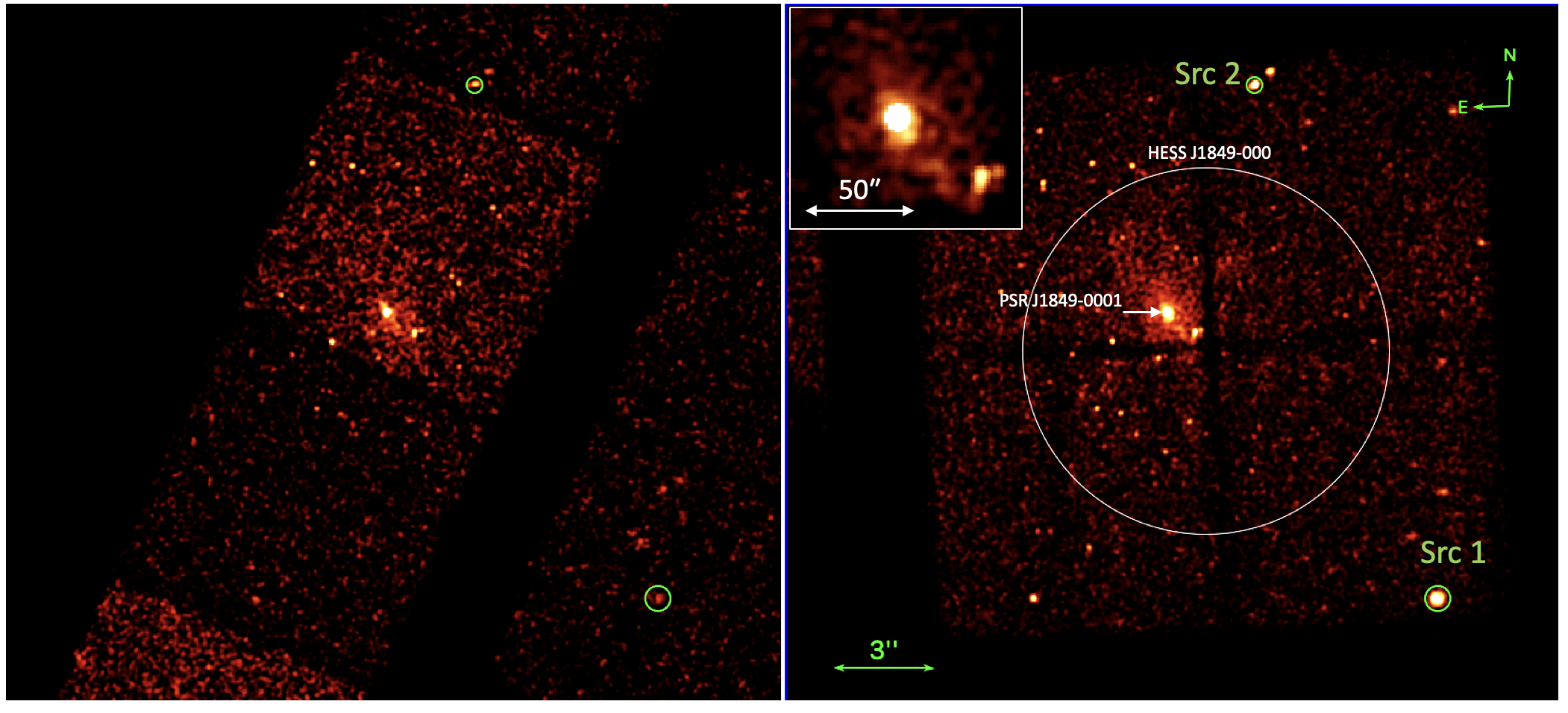
Figure 1: The ACIS-S (left; ObsID 13291) and ACIS-I (right; ObsIDs 23596, 24494, and 24495 combined) images of the HESS J1849–000 field (the size of the TeV source is shown by the white circle) in 0.7-7 keV. The inset shows zoomed-in view of the brighter part of PWN powered by PSR J1849–0001. Two green circles labeled Src 1 and Src 2 show two brightest (in the combined ACIS-I image) sources.

3 RESULTS

3.1 Images

Figure 1 shows the X-ray view of the HESS J1849–000 field as seen by ACIS-S and ACIS-I observations. The PWN is better discernible in the combined ACIS-I image because of the longer exposure and lower ACIS-I background. The merged ACIS-I image reveals a compact PWN consisting of an elongated structure extending to the southwest of the pulsar: likely a pulsar jet exhibiting helicity. In addition to the bright compact PWN (the jet; see the inset in Figure 1), fainter and more extended PWN emission is seen northeast of the pulsar.

A number of point sources are seen in the images with the two most prominent (brightest) ones (Source 1 = CXOU J184829.9–000943 and Source 2 = CXOU J184851.2+000523) marked by the green circles in the ACIS-I image. We note that Source 1 is strongly variable.

The top panel in Figure 2 shows the image produced by applying exposure-map corrections and subtracting point sources. CIAO’s wavdetect (Freeman et al., 2002) was used to detect the point sources and their respective background regions were created by roi. The point sources were then replaced with background regions using dmfilth, creating a diffuse emission image. The exposure–correction was performed by dividing the diffuse emission image by the exposure map with dmimgcalc. The individual images and exposure map were binned by a factor of two. The resulting images from each observation are then combined (using dmimgcalc) and the result was smoothed with aconvolve. The putative helical jet extending SW of the pulsar is more apparent in this exposure-corrected diffuse emission image.

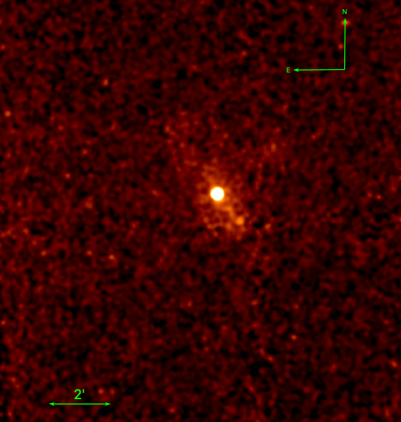
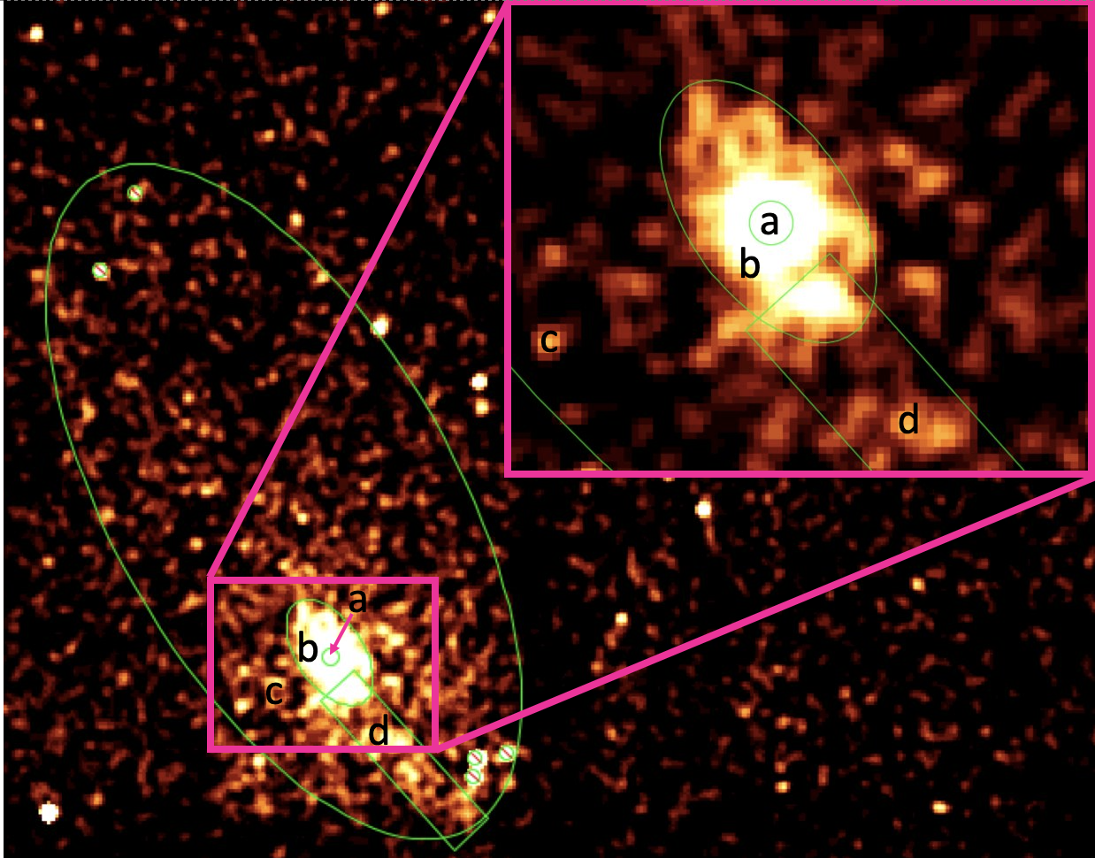
Figure 2: The top panel shows the point source subtracted and exposure-map corrected image of the J1849 PWN. The image is binned by a factor of 4 and smoothed with a two-pixel Gaussian kernel. The bottom panel shows regions used for spectral extractions: A – Pulsar ($r=3.0^{\prime\prime}$), B – Inner PWN, C – Extended PWN, D – jet candidate.

3.2 Pulsar motion

Once the astrometry in the individual observations was corrected, as described in the Appendix, we measured the proper motion from the images. We used a standard centroiding approach (described in e.g. Da Costa 1992) to measure pulsar positions for $r=0.37^{\prime\prime}$, $0.49^{\prime\prime}$, and 0.61^′′ circular apertures in ObsID 13291 and 24494 which are separated by 3,590 days. These two positions differ by $-0.16^{\prime\prime}$ in R.A and $-0.03^{\prime\prime}$ in Decl. Since this difference is noticeably smaller than the weighted root-mean-square residuals (WRMSR) after the astrometric alignment (see Table 3 in the Appendix), we conclude that the pulsar’s proper motion could not be detected with the existing data. We note that the weighted root-mean-square residual of $0.18^{\prime\prime}$ (see Appendix) corresponds to $\approx 600$ km s^-1 at the fiducial distance of 7 kpc. This can be taken as an upper limit on pulsar’s velocity.

3.3 PWN and Pulsar Spectra

The bottom panel in Figure 2 shows regions used for spectral extraction on top of the combined (from all 4 observations) ACIS image. The pulsar’s spectrum was extracted from $r=3.0^{\prime\prime}$ circular aperture centered at the brightest pixel (region A in Figure 2, lower panel), which corresponds to $\approx 90$% encircled PSF fraction at 1.5 keV. This radius was chosen by studying the pulsar contribution to the Inner PWN region. The net counts in the Inner PWN region in the X-ray image were compared to the net counts in that region from a point source simulated using MARX at varying radii (Davis et al., 2012). Using the chosen aperture the pulsar contributes about 30% to the Inner PWN.

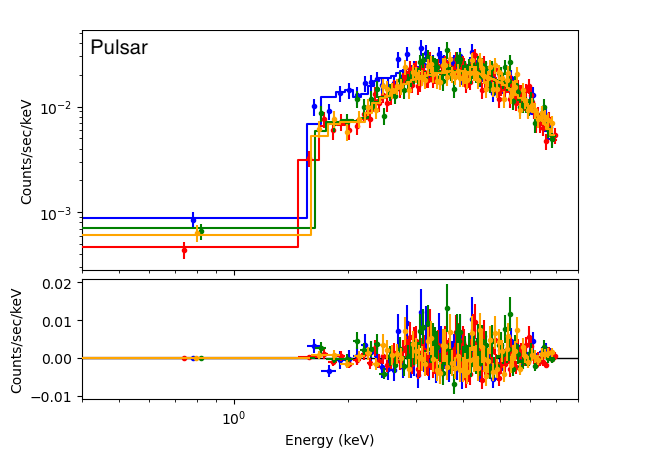
Figure 3: Spectrum of PSR J1849-0001. Different colors represent each observation (blue – 13291, red – 23596, green – 24494, orange – 24495.

To fit the pulsar spectrum (shown in Figure 3) we first grouped counts by requiring $\geq 30$ counts per bin and restricted the energy range to 0.5 – 7.0 keV. The PL model, modified by interstellar absorption, provides a good fit with a reduced chi-squared $\chi_{\nu}^{2}$=1.03 for $\nu=$311 degrees of freedom (d.o.f.). The best-fit PL $\Gamma=1.20\pm 0.07$ while $n_{\rm H}=4.40\times 10^{22}$ cm^-2. The corresponding absorbed and unabsorbed fluxes are $(2.0\pm 0.2)\times 10^{-12}$erg cm^-2 s^-1 and $3.9\begin{subarray}{c}+1.3\\ -1.5\end{subarray}\times 10^{-12}$erg cm^-2 s^-1, respectively. The unabsorbed luminosity at the assumed $d=7$ kpc, is $(2.3\pm 0.1)\times 10^{34}$erg s^-1. The $n_{\rm H}$ inferred from the PL fit to the pulsar’s spectrum is used in the PWN fits below.

Using the same grouping and energy range as for the pulsar ($\geq 30$ counts per bin, 0.5 – 7.0 keV), we divided the PWN into several regions (see Figure 2, bottom panel) in order to look for spectral changes (e.g., due to radiative cooling) and to isolate and measure the compact PWN spectrum which should be less affected by cooling, and hence, offers a better probe of the injected particle spectral energy distribution (SED).

Region B encloses the brighter Inner (more compact) PWN with Region A being excluded. The large-scale Extended PWN spectrum is extracted from region C with region B being excluded. Within Region C, there are several point sources that have been also excluded from the extended PWN region. The putative pulsar jet is enclosed by region D. Two background regions were selected nearby, but sufficiently outside of Region D, to minimize the contamination from the extended PWN, in a region overlapped by all observations.

Since the PWN emission is relatively faint and significantly contaminated by the background, we fix $n_{\rm H}$ at the value determined from the fit to the bright pulsar. We note the pulsar spectrum has very few photons below 1.5 keV and, hence, even if it has a thermal soft (see, e.g., Kargaltsev & Pavlov 2007) component unaccounted in the PL fit, it is unlikely to have any noticeable impact on the determination of $n_{\rm H}$. The measured large $n_{\rm H}$ value is consistent with the presence of a dark cloud apparent in optical survey images; e.g., Pan-STARRS (Chambers & et al., 2017), which must be located at a 0.5-0.7 kpc distance based on the scarcity of foreground stars and on the 3D dust distribution map (Green et al., 2019). Thus, the cloud is likely in front of the pulsar.

The Inner PWN spectrum (shown in Figure 4) is hard with the best-fit $\Gamma=1.19\pm 0.14$ and $\chi^{2}_{\nu}$=1.09 for $\nu=$25. The absorbed and unabsorbed fluxes are $(1.3\pm 0.1)\times 10^{-13}$erg cm^-2 s^-1 and $(2.7\pm 0.2)\times 10^{-13}$erg cm^-2 s^-1, respectively. The unabsorbed luminosity is $(1.5\pm 0.1)\times 10^{33}$erg s^-1. The PL fit to the spectrum from a much larger Extended PWN region can be described by a PL with $\Gamma=1.56\pm 0.11$ with $\chi^{2}_{\nu}$=1.0 for $\nu=$188. The absorbed and unabsorbed fluxes are $(4.8\pm 0.2)\times 10^{-13}$erg cm^-2 s^-1 and $11.5\begin{subarray}{c}+0.6\\ -0.8\end{subarray}\times 10^{-13}$erg cm^-2 s^-1, respectively, and the unabsorbed luminosity is $6.7\begin{subarray}{c}+0.4\\ -0.5\end{subarray}\times 10^{33}$erg s^-1. Finally, we attempted to fit separately the spectrum from a possible pulsar jet region and obtained a somewhat larger, albeit uncertain, $\Gamma=1.70\pm 0.22$. The fit quality is rather poor with $\chi^{2}_{\nu}$=2.01 for $\nu=$16. Therefore, we cannot say whether the spectrum from the putative jet region is any different from the surrounding emission spectrum.

Table 1: Observed and Derived Pulsar Parameters

Parameter	Value
R.A. (J2000.0)	18:49:01.632 (40)
Dec. (J2000.0)	–00:01:17.45 (60)
Epoch of Position (MJD)	55,885
Galactic Longitude (deg)	32.64
Galactic Latitude (deg)	0.53
Spin Period, $P$ (ms)	38.52 (15)
Period Derivative, $\dot{P}$ (10-15)	14.16 (11)
Surface Magnetic Field, $B_{S}$ (1011 G)	7.47
Spin-Down Power, $\dot{E}$ (1036 erg s-1)	9.8
Spin-Down Age, $\tau_{sd}$ = P/(2$\dot{P})$ (kyr)	43.1

Table 2: Spectral Fit Results for PWN Regions and Point Sources

Region	Name	Area	Counts	$\Gamma$	$\mathcal{N}_{-5}$	$\chi_{\nu}^{2}$ ($\nu$ d.o.f.)	$F_{-13}$	$F_{-13}^{\rm unabs}$
a	Pulsar	28	$10673\pm 103$	$1.20\pm 0.07$	$46.18\pm 5.04$	1.03 (311)	$19.72\begin{subarray}{c}+0.24\\ -0.25\end{subarray}$	$38.70\begin{subarray}{c}+1.33\\ -1.55\end{subarray}$
b	Inner PWN	687	$792\pm 30$	$1.36\pm 0.14$	$3.86\pm 0.73$	1.09 (25)	$1.27\pm 0.06$	$2.72\begin{subarray}{c}+0.16\\ -0.21\end{subarray}$
c	Extended PWN	22476	$3026\pm 96$	$1.56\pm 0.11$	$19.47\pm 2.93$	1.0 (188)	$4.78\pm 0.18$	$11.46\begin{subarray}{c}+0.63\\ -0.79\end{subarray}$
d	Pulsar Jet	1054	$437\pm 24$	$1.70\pm 0.22$	$3.40\pm 0.99$	2.01 (16)	$0.66\begin{subarray}{c}+0.05\\ -0.06\end{subarray}$	$1.78\begin{subarray}{c}+0.20\\ -0.26\end{subarray}$
e	Src 1 (13291)	706	$32\pm 7$	–	–	–	$0.26\pm 0.08$	–
e	Src 1 (23596)	706	$421\pm 21$	$1.34\pm 0.18$	$7.41\pm 1.83$	1.37 (12)	$2.62\begin{subarray}{c}+0.18\\ -0.19\end{subarray}$	$5.37\begin{subarray}{c}+0.37\\ -0.51\end{subarray}$
e	Src 1 (24494)	706	$310\pm 18$	$1.60\pm 0.21$	$12.18\pm 3.28$	1.33 (8)	$2.89\begin{subarray}{c}+0.21\\ -0.24\end{subarray}$	$6.90\begin{subarray}{c}+0.63\\ -0.83\end{subarray}$
e	Src 1 (24495)	706	$126\pm 12$	$1.39\pm 0.36$	$3.78\pm 1.82$	0.78 (2)	$1.18\begin{subarray}{c}+0.16\\ -0.20\end{subarray}$	$2.57\begin{subarray}{c}+0.31\\ -0.54\end{subarray}$
f	Src 2 (13291)	312	$32\pm 6$	–	–	–	$0.11\pm 0.03$	–
f	Src 2 (23596)	312	$168\pm 13$	$2.80\pm 0.19$	$6.71\pm 1.18$	1.27 (4)	$0.68\pm+0.06$	$2.06\pm 0.29$
f	Src 2 (24494)	312	$63\pm 8$	–	–	–	$0.46\pm 0.10$	–
f	Src 2 (24495)	312	$121\pm 11$	$2.37\pm 0.25$	$5.35\pm 1.26$	1.0 (2)	$0.81\pm+0.09$	$1.90\begin{subarray}{c}+0.28\\ -0.26\end{subarray}$

PWN spectral fits are performed jointly (all 4 ACIS observations are included). The different regions of the PWN are shown in Figure 2, bottom panel. Listed are the region name, area (in arcsec²), net counts, photon index $\Gamma$, PL normalization $\mathcal{N}_{-5}$ in units of $10^{-5}$ photons s^-1 cm^-2 keV^-1 at 1 keV, reduced $\chi^{2}_{\nu}$ ($\nu$ d.o.f.), and absorbed and unabsorbed 0.5–7 keV fluxes in units of $10^{-13}$ erg cm^-2 s^-1. In all fits for the PWN we set $n_{\rm H}=4.40\times 10^{22}$ cm^-2. The fits to Src 1 and Src 2 spectra are performed for each ObsID (listed in parentheses) individually because these sources are variable. For Source 1 $n_{\rm H}=(3.87\pm 0.90)\times 10^{22}$ cm^-2 and for Source 2 $n_{\rm H}=(0.82\pm 0.43)\times 10^{22}$ cm^-2. Src 1 (13291), Src 2 (13291), and Src 2 (24494) did not have enough data for a meaningfully constrained spectral fit. The absorbed fluxes of the point sources Src 1 (13291) & 2 (13291, 24494) were obtained from the Chandra Source Catalog (v.  2.0.1; Evans et al. 2020).

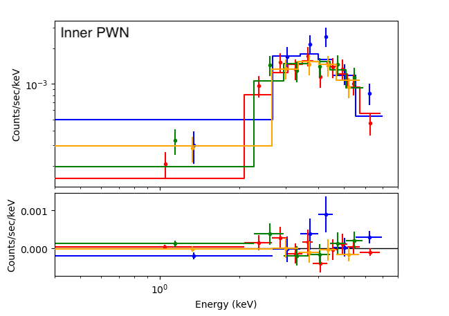
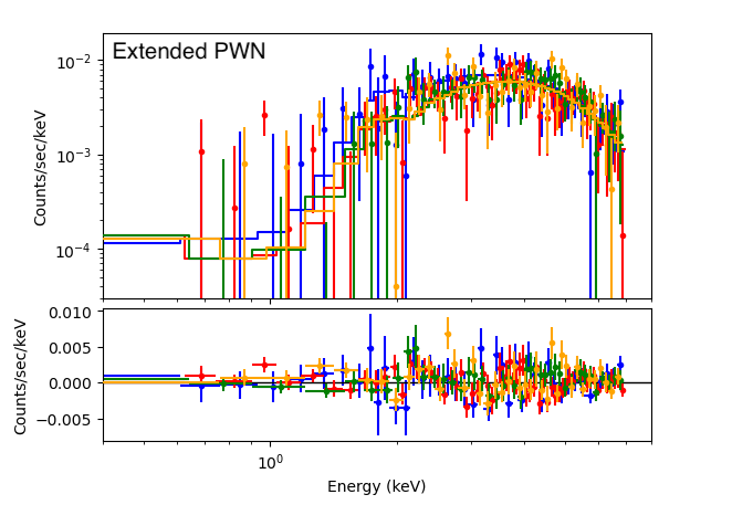
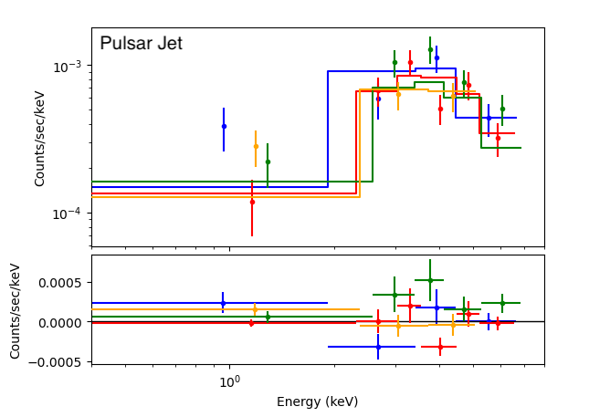
Figure 4: Spectra of the PWN around PSR J1849-0001.

3.4 Brightest Field Sources

We also analyzed the spectra of the two brightest unresolved X-ray sources shown in Figure 1: Src 1=CXOU J184829.9-000943 ($\alpha=282.1248^{\circ}$, $\delta=-0.1620^{\circ}$; 1$\sigma$ uncertainty $\approx 1.4^{\prime\prime}$) and Src 2=CXOU J184851.2+000523 ($\alpha=282.2137^{\circ}$, $\delta=0.0898^{\circ}$; 1$\sigma$ uncertainty $\approx 0.7^{\prime\prime}$). Both sources were imaged on ACIS-I (ObsIDs 23596, 24494, and 24495) and ACIS-S chips (ObsID 13291). However, due to their variability and different sensitivity of the ACIS-S detector they are not the brightest in the ACIS-S image. The spectra of both sources (shown in Figure 6) fit satisfactory an absorbed PL model with $n_{\rm H}=(3.9\pm 0.9)\times 10^{22}$ cm^-2 and $n_{\rm H}=(8.2\pm 4.3)\times 10^{21}$ cm^-2 for Src 1 and Src 2, respectively (see Table 2 for details). Src 1 is strongly variable (see Figure 5). Its flux changed from $(2.9\pm 0.2)\times 10^{-13}$erg cm^-2 s^-1 to $(1.2\pm 0.2)\times 10^{-13}$erg cm^-2 s^-1 between 2021 September 26 and 2022 September 11. The source does not have optical/NIR counterparts in 2MASS, Gaia DR3, or AllWISE catalogs. However, the more sensitive PanSTARRS DR1 (Chambers & et al., 2017) and UKIDSS DR6 (UKIDSS Consortium, 2012) surveys show that Src 1 is located in a fairly crowded environment with several sources within a few arcseconds radius. The closest potential counterpart to Src 1 is an optical/IR source detected by PanSTARRS DR1 (with zmag=19.4 and ymag=18.5) and UKIDSS DR6 (with jmag=16.3, hmag=15.4, and k1mag=14.9) separated by 1.5$\arcsec$ from X-ray source. If the association is true, the red color of the counterpart and the X-ray brightness makes Src 1 a promising AGN candidate. Src 1 is not detected in radio surveys including VLASS (Lacy et al., 2020) and RACS (McConnell et al., 2020) but some AGN are radio-quiet/faint. Src 2 is also variable by a factor of 4 with the lowest flux being recorded during ObsID 13291. It varies by a factor of 2 among the 3 more recent observations with no clear evidence of a flare within either of the observations. Within its error ellipse, Src 2 is coincident with two Gaia DR3 sources 4266382197008542592 and 4266382196999393920 which are offset by $0.42^{\prime\prime}$ and $0.55^{\prime\prime}$, respectively. Both optical sources have similar proper motion (in terms of direction and magnitude) and are located at the same (within the uncertainties) distance of $\approx$700 pc. Therefore, they may be components of a binary system with an orbital separation of about 420 AU. The observed ACIS-I fluxes correspond to the unabsorbed luminosities of $(0.4-2)\times 10^{31}$ erg s^-1. Src 2 is also not detected in radio surveys including VLASS (Lacy et al., 2020) and RACS (McConnell et al., 2020).

For the brighter Src 1 we performed a periodicity search in 3 ACIS-I observations (individually, after applying barycentric correction with CIAO’s axbary) using the $Z_{n}^{2}$ test (for the number of harmonics n=1, 2; Buccheri et al. 1983) in the $2\mathrm{T_{\rm obs}}^{-1}-0.15625$ Hz frequency range, where $T_{\rm obs}$ is the observation duration. The frequency resolution was taken to be a factor of 50 smaller than $1/T_{obs}$. No significant periodicity was discovered in any of the observations except for a hint of $\sim 12$ ks periodicity in the data from ObsID 23596 (see the top panel of Figure 5) which is not statistically significant in these data.

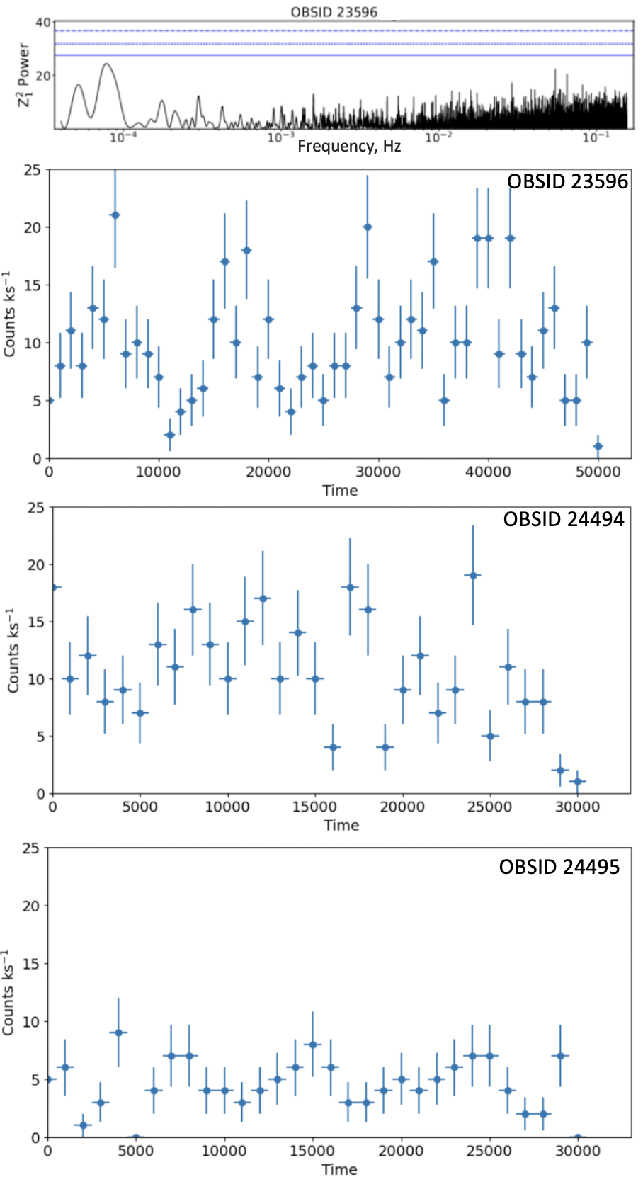
Figure 5: Lightcurves of CXOU J184829.9-000943 from 3 ACIS-I observations (three bottom panels) at 1 ks binning. The top panel shows $Z_{n}^{2}$ as a function of frequency. The highest peak, at $\approx 80$ $\mu$Hz, corresponds to the hint of periodicity seen in the first half of lightcurve from ObsID 23956.

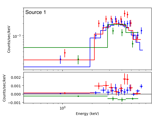
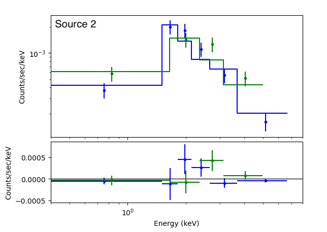
Figure 6: Spectra of point sources (Src 1 & 2) found in the CXO ACIS observations (ObsIDs: 13291, 23596, 24494, 24495). Different colors represent each observation (blue – 23596, red – 24494, green – 24495)

4 Discussion

The deep ACIS images revealed that the PWN of PSR J1849–0001 has rather amorphous morphology and does not belong to the torus-jet (with the torus being dominant) type of PWNe like those powered by Crab or Vela pulsars. If the faint structure extending SW of the pulsar is indeed a jet then it may rather resemble PWNe in young Kes 75 or SNR G11.2-0.3 SNRs where only one of the two jets is clearly seen (see Figure 7). The one-sidedness can be explained by the pulsar spin axis (also jet direction) pointing close to the line-of-sight. In this case the jet emission is Doppler-boosted while the counter-jet emission is de-boosted. The evidence for a jet and the lack of discernible torus also suggests that the inclination angle $\alpha$ between the magnetic and spin axis is small (Bühler & Giomi, 2016).

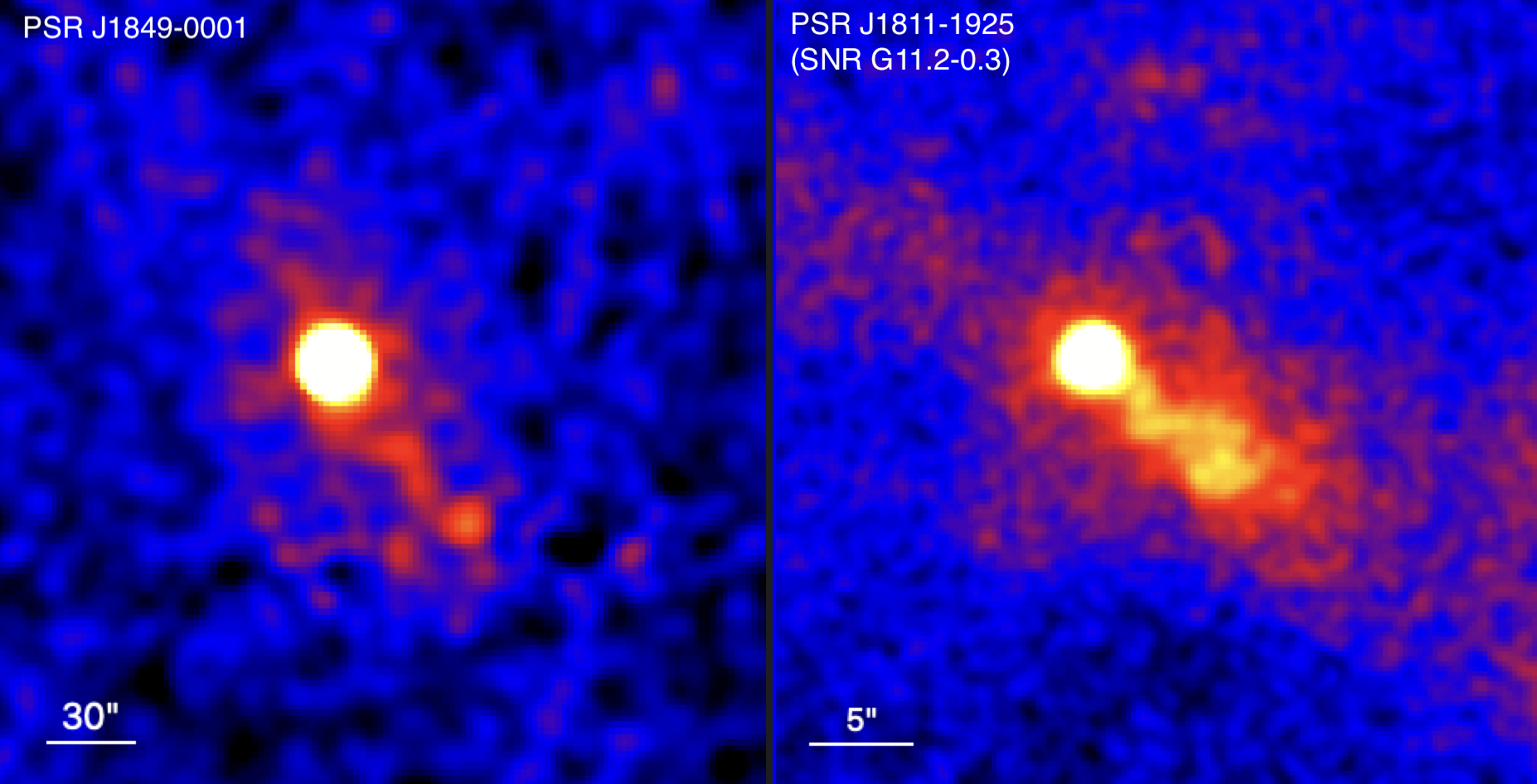
Figure 7: Comparison of PWNe produced by the PSRs J1849–0001 and PSR J1811-1925 (in SNR SNR G11.2-0.3). The latter pulsar is also young ($\sim 2$ kyr) and energetic ($6.5\times 10^{36}$ erg s^-1) with $P=64$ ms. Its compact PWN appearance is dominated by a helical jet.

The compact (Inner) PWN luminosity (region B in Figure 2) is $\approx 1.6\times 10^{33}$ erg s^-1 in 0.5–7 keV (at $d=7$ kpc), or, $\approx 1.6\times 10^{-4}\dot{E}$, which is below typical X-ray efficiencies of PWNe produced by similarly energetic pulsars (see e.g., Figure 2 in Kargaltsev et al. 2013). The Extended PWN spectrum is softer than that of the inner PWN. The softening can be attributed to the radiative (synchrotron) energy losses which would then imply a spectral break and a flatter Extended PWN spectrum at lower frequencies.

The combined (from regions B and C) X-ray luminosity $L_{X}\approx 8.3\times 10^{33}$ erg s^-1 corresponds to the radiative efficiency $\eta_{X,{\rm pwn}}=L_{X}/\dot{E}\approx 8.5\times 10^{-2}$. In comparison, the HESS J1849–000 TeV luminosity, $L_{\rm TeV}\approx 1.2\times 10^{34}$ erg s^-1 (in 1–10 TeV), corresponds to the TeV radiative efficiency of $1.2\times 10^{-3}$, which are fairly typical values for TeV PWNe (H. E. S. S. Collaboration et al., 2018a). We note that, unlike X-ray efficiency, the TeV efficiency is not contemporaneous because the cooling time of TeV emitting particles is about a factor of 10 longer (at 1 TeV) and, hence, the pulsar’s $\dot{E}$ may have been significantly larger when the TeV-emitting particles were injected. Amenomori et al. (2023) measured the spectrum of HESS J1849-000 at TeV energies and found no evidence of cut-off up to $E_{\gamma}=740$ TeV. For the IC on CMB photons this implies the corresponding electron energy of $E_{e}\approx 2.15(E_{\gamma}/1~{}{\rm PeV})^{0.77}=1.7$ PeV (Amenomori et al., 2023). This energy corresponds to $\sim 30$% of the energy, $e\left(\dot{E}/c\right)^{1/2}$ corresponding to the current potential drop across the polar cap of PSR J1849-0001. However, it is important to note that in the past the pulsar’s $\dot{E}$ was larger.

Since HESS J1849–000 is relatively compact compared to some other TeV sources associated with PWNe, we attempted to model the multiwavelength spectrum with a simple one-zone (leptonic) radiation model using the Python package naima (Zabalza, 2015). We first modeled the electron SED with an exponential cut-off power law $N(E)=A(E/E_{0})^{-p}\exp(-(E/E_{\rm max})^{\beta})$, where $A$ is the normalization (in units of particles GeV^-1 at 1 GeV), $E_{0}$ is the reference energy (1 GeV), $p$ is the slope of the electron SED, $E_{\rm max}$ is the maximum particle energy, and $\beta$ is the cutoff exponent (which we set to 10 to quickly kill off the SED above the maximum energy). The slope of the electron SED, $p=2.04$, is inferred from the photon index, $\Gamma=1.52$, for the absorbed PL model fitted to all PWN regions combined together assuming optically thin synchrotron emission.

The observed X-ray spectrum requires a maximum electron energy of at least $E_{\rm max}=600$ TeV. The minimum electron energy, chosen to be $E_{\rm min}=E_{0}=1$ GeV (the Naima default, is not known. However, it does not correlate with other model parameters and does not change the fit as long as it is small enough). For the IC spectrum, we use the background photon fields from Popescu et al. (2017): the CMB, a far-IR component ($T=30$ K, $U=2\times 10^{-12}$ erg cm^-3), a near-IR component ($T=500$ K, $U=4\times 10^{-13}$ erg cm^-3), and a visible component ($T=5000$ K, $U=1.5\times 10^{-12}$ erg cm^-3). We varied the values of $B$, $E_{max}$, and normalization $A$ until we obtained a reasonably good match between the model and the data (see Figure 8). However, the inferred value of the magnetic field, $1-2$ $\mu$G is low even when compared to the typical Galactic plane field ($\sim 5$ $\mu$G; Ferrière 2015). This may be an artifact of using a simplistic one-zone model that does not include the expected spectral evolution causing the SED of older particles to be different from that of the freshly injected ones (e.g., due to the radiative cooling) nor does it account for a possible large variation of $B$ with the distance from the pulsar or a variable particle injection rate of particles throughout the life of the pulsar. We note that the radiative losses are expected to produce a cooling break in the spectrum (see, e.g., discussion of cooling breaks in Klingler et al. 2018). Although the location of the break is currently unconstrained (the radio upper limit is too high; see Fig. 8), placing it at a reasonable energy (based on other young PWN, e.g., the Crab, Vela, or Mouse PWNe spectra where such a break is constrained) does not affect the inferred values of the magnetic field and $E_{\rm max}$. We also note that, for this source, the simplistic one-zone model could perform better here than for some other large TeV/X-ray PWNe (e.g., Li et al. 2023) because for HESS J1849-000 the TeV source size is comparable to the X-ray PWN size (see Figure 9). Despite this, the simplistic one-zone model may be lacking in that it is not accounting for the presence of an older “relic” electron population which is no longer emitting synchrotron emission in X-rays, but which could still be emitting inverse-Compton emission in TeV gamma-rays (as IC cooling timescales ($\sim$ 10 kyr) are an order of magnitude longer than synchrotron cooling timescales ($\sim$ 1 kyr) for typical PWN parameters). In the presence of a relic PWN, the PWN magnetic field would be raised to a more realistic value (e.g., $B\gtrsim 20\ {\rm\mu G}$). Finally, we note that although Amenomori et al. (2023) discussed an alternative hadronic scenario, where the TeV $\gamma$-rays are produced by neutral pion decay, no evidence of a radio SNR is seen the radio images (see Figure 9). We defer the more detailed modeling to a future publication.

Figure 8: Multiwavelength SED of the J1849 PWN. Shown are the data from: Chandra (this paper), Fermi-LAT (upper limits Eagle 2022), HESS (H. E. S. S. Collaboration et al., 2018b), LHAASO (Cao et al., 2021), and the Tibet Air Shower Array (TASA; Amenomori et al. 2023). The curves show synchrotron (blue) and IC (red) emission from a PL (solid) and a broken PL (dashed) electron SED in a one-zone PWN model. The $2\sigma$ GLOSTAR survey limit (at 6.9 GHz; Brunthaler et al. 2021) is shown assuming the radio source to be as large as TeV source. The survey’s angular resolution is $18^{\prime\prime}$. Note that the survey’s largest resolvable angular scale is $4^{\prime}$ which is a factor of 2 smaller than the TeV source size (see Figure 9). Therefore, the upper limit is very approximate. The limit from the VLA GPS is significantly higher (not shown for this reason) although GPS can resolve larger angular scales than the GLOSTAR survey.

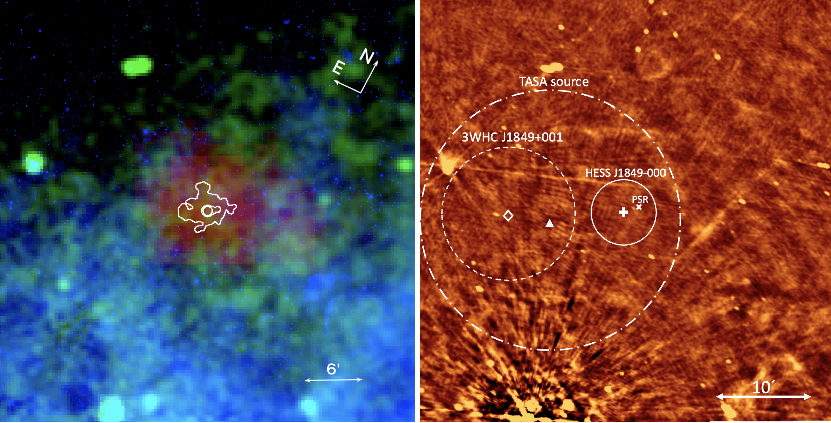
Figure 9: The left panel shows the true-color image: red - TeV from HESS GPS (H. E. S. S. Collaboration et al., 2018b), green - 1.42 GHz continuum radio from VLA Galactic Plane Survey (Stil et al., 2006), blue - Spitzer IRAC 8 micron image from GLIMPSE 360 survey (Churchwell et al., 2009). The contours are X-rays based on the image shown in the top panel of Figure 1. The right panel is the 6 GHz radio image from the GLOSTAR survey (Brunthaler et al., 2021) showing the same area of the sky as in the left panel. For the HESS source, the solid circle shows the extent of the source (H. E. S. S. Collaboration et al., 2018b). For the 3HWC source, the dashed circle shows the positional uncertainty (systematic and $1\sigma$ statistical combined; Albert et al. 2020). The dash-dotted circle shows the positional uncertainty of the VHE source detected by the Tibet Air shower array (systematic and $1\sigma$ statistical combined; Amenomori et al. 2023) .

For the pulsar $L_{X}\approx 2.3\times 10^{34}$ erg s^-1 and the radiative efficiency $\eta_{X,{\rm psr}}\approx 2.3\times 10^{-3}$. The latter is in line with values typically seen in young pulsars. It is important to note that PSR J1849–0001 has not been detected in radio or in $\gamma$-rays. Among 65 pulsars with $\dot{E}>10^{36}$ erg s^-1 only 8 pulsars are both radio and $\gamma$-ray quiet. In fact, there is only one pulsar with $\dot{E}$ higher than that of PSR J1849–0001 that is radio and $\gamma$-ray quiet (J1813–1749 in SNR 12.8–0.0; also an INTEGRAL source). It is a bit of a mystery why some young high-$\dot{E}$ pulsars exhibit pulsations in X-rays / soft $\gamma$-rays, but are quiet (or very weak) in radio and $\gamma$-rays. It is not that particle acceleration and pair creation are inefficient in these pulsars because their X-ray luminosities are not unusual. A more likely explanation is a specific magnetospheric geometry – the combination of angle ($\alpha$) between the magnetic dipole and spin axis and/or an unfavorable viewing angle ($\zeta$) – makes the narrow radio beam and the $\gamma$-ray emission from the outer magnetosphere miss the Earth, while the broader beam of non-thermal X-ray emission from pairs above the polar cap is still seen. In this respect, a similar case could be that of another $\gamma$-ray- and radio-quiet pulsar PSR J1811–1925 (Torii et al., 1997) where deep CXO observations (Borkowski et al., 2016) also revealed an underluminous compact PWN with clear evidence of jet but only a weak indication of a torus. The 3-8 keV pulse profiles of PSR J1849–0001 (Bogdanov et al., 2019) and PSR J1811–1925 (Madsen et al., 2020) are also similar, showing a single broad peak per rotation period. One of the possible consequences of such a geometry is the relative faintness of the PWN because for a more aligned rotator a smaller volume is occupied by the striped pulsar wind zone where the magnetic field energy is converted to the energy of pulsar wind particles. We also note that pulsars having small $\alpha$ are not expected to be weak gamma-ray sources lacking pulsations (see e.g., Cerutti et al. 2016).

5 Conclusions

CXO observations show that young and energetic PSR J1849–0001 is surrounded by an underluminous compact PWN which lacks the often-seen torus-jet morphology. The combined CXO image shows amorphous PWN morphology with some evidence of a jet and no evidence of a torus. Morphologically, the PWN of PSR J1849–0001 may resemble the brighter PWN of PSR J1811–1925. Both of these pulsars feature hard non-thermal spectra, are gamma-ray and radio-quiet, have similar pulse profiles in X-rays, and also have similar spin-down properties. Both pulsars also belong to the so-called MeV pulsar class which could nave small inclination angles between the spin and magnetic dipole axis.

The fainter extended X-ray PWN is discernible up to a few arcminutes in the combined CXO images. This PWN is one of the few where the connection between the TeV (HESS J1849–000) and X-ray PWNe is credible because of the good positional coincidence and relative compactness of the TeV source. The comparable sizes of the X-ray and TeV PWNe could make the simplistic one-zone modeling more relevant than in some other X-ray/TeV PWN cases. However, the inferred magnetic field value is still suspiciously low suggesting that even in such cases the dynamics of particle injection and varying magnetic fields are likely to have a large impact on the observed PWN emission.

We also find a curiously bright and variable X-ray source which is apparently associated with a very wide binary that is not expected to show any additional X-ray activity due to the large separation between the stars. The X-ray lightcurves do not show flares typical of coronally active stars. Optical spectroscopy could help to better understand the type of star(s) and underlying reasons for X-ray activity.

Appendix A Astrometry

We perform both relative astrometry by aligning X-ray sources from individual observations, and absolute astrometry by tying X-ray source positions in the merged image to optical counterparts in the Gaia DR3 catalog (Gaia Collaboration et al., 2023).

The CIAO tool wcs_match is used to determine the translational shift minimizing the sum of positional offsets between the matched pairs. The 1$\sigma$ uncertainty of the astrometric correction is calculated using the weighted root-mean-square residual (WRMSR) as

$${\rm WRMSR}^{2}=\frac{\sum_{i=1}^{N}w_{i}R_{i}^{2}}{\sum_{i=1}^{N}w_{i}}$$ (A1)

with

$$w_{i}=\frac{1}{\sigma_{i}^{2}}=\frac{1}{\sigma_{{\rm ref},i}^{2}+\sigma_{{\rm X},i}^{2}}$$ (A2)

where $R_{i}$ is the residual for the $i$th pair after the astrometric correction, and $\sigma_{{\rm ref},i}$ and $\sigma_{{\rm X},i}$ are the positional uncertainties of the reference source and the X-ray source to be aligned with of the $i$th pair.

To find optimal parameters for wcs_match and ensure the reliability of matched pairs for astrometric correction, we perform wcs_match on a grid of search radii and residual limits. We select values yielding $\geq 5$ matched pairs, with astrometric correction (and its uncertainty WRMSR) consistent with most solutions from the parameter space grid search. For relative astrometry, we use significant X-ray sources (detection significance $>3\sigma$ and net counts $>$10) detected from wavdetect (Freeman et al., 2002), excluding the pulsar, to co-align the reference X-ray image (ObsID=23596) and the other three images. Corrected (with wcs_update) images are co-added to create a deeper merged image using CIAO task merge_obs. For absolute astrometry, a more stringent selection ($\sigma>5$ and net counts $>$20) is applied to X-ray sources detected from the merged image before aligning them to Gaia DR3 sources. Finally, we update the WCS information and the aspect history files accordingly using wcs_update. The relative and absolute astrometry solutions are summarized in the first and second parts of Table 3.

ObsID	radius1	reslim2	$\Delta$RA(′′)	$\Delta$DEC(′′)	WRMSR(′′)	# of pairs
13291	0.6	0.45	-0.23	0.40	0.18	7
24494	1.6	0.5	-0.21	1.36	0.27	6
24495	0.7	0.6	0.01	-0.16	0.28	9
merged	1.0	0.4	0.07	-0.25	0.27	6

Table 3: The relative astrometry solutions in the first part of the table with the reference ObsID=23596 and the absolute astrometry solution (corrected to Gaia DR3) in the second part of the table. ¹ – Source match radius for wcs_match; ² – Residual limit for wcs_match.

References

- Abeysekara et al. (2017) Abeysekara, A. U., Albert, A., Alfaro, R., et al. 2017, ApJ, 843, 40. doi:10.3847/1538-4357/aa7556
- Albert et al. (2020) Albert, A., Alfaro, R., Alvarez, C., et al. 2020, ApJ, 905, 76. doi:10.3847/1538-4357/abc2d8
- Amenomori et al. (2023) Amenomori, M., Asano, S., Bao, Y. W., et al. 2023, ApJ, 954, 200. doi:10.3847/1538-4357/acebce
- Anderson et al. (2017) Anderson, L. D., Wang, Y., Bihr, S., et al. 2017, A&A, 605, A58. doi:10.1051/0004-6361/201731019
- Bai & Spitkovsky (2010) Bai, X.-N. & Spitkovsky, A. 2010, ApJ, 715, 1282. doi:10.1088/0004-637X/715/2/1282
- Balucinska-Church & McCammon (1992) Balucinska-Church, M. & McCammon, D. 1992, ApJ, 400, 699. doi:10.1086/172032
- Bogdanov et al. (2019) Bogdanov, S., Ho, W. C. G., Enoto, T., et al. 2019, ApJ, 877, 69. doi:10.3847/1538-4357/ab1b2e
- Borkowski et al. (2016) Borkowski, K. J., Reynolds, S. P., & Roberts, M. S. E. 2016, ApJ, 819, 160. doi:10.3847/0004-637X/819/2/160
- Brunthaler et al. (2021) Brunthaler, A., Menten, K. M., Dzib, S. A., et al. 2021, A&A, 651, A85. doi:10.1051/0004-6361/202039856
- Stephen et al. (2006) Stephen, J. B., Bassani, L., Malizia, A., et al. 2006, A&A, 445, 869. doi:10.1051/0004-6361:20053958
- Buccheri et al. (1983) Buccheri, R., Bennett, K., Bignami, G. F., et al. 1983, A&A, 128, 245
- Bühler & Giomi (2016) Bühler, R. & Giomi, M. 2016, MNRAS, 462, 2762. doi:10.1093/mnras/stw1773
- Cao et al. (2021) Cao, Z., Aharonian, F. A., An, Q., et al. 2021, Nature, 594, 33. doi:10.1038/s41586-021-03498-z
- Cerutti et al. (2016) Cerutti, B., Philippov, A. A., & Spitkovsky, A. 2016, MNRAS, 457, 2401. doi:10.1093/mnras/stw124
- Chambers & et al. (2017) Chambers, K. C. & et al. 2017, VizieR Online Data Catalog, II/349
- Churchwell et al. (2009) Ed Churchwell et al 2009 PASP 121 213. doi:10.1086/597811
- Da Costa (1992) Da Costa, G. S. 1992, Astronomical CCD Observing and Reduction Techniques, 23, 90
- Davis et al. (2012) Davis, J. E., Bautz, M. W., Dewey, D., et al. 2012, Proc. SPIE, 8443, 84431A. doi:10.1117/12.926937
- Eagle (2022) J. Eagle, 2022, arXiv:2209.11855v1 [astro-ph.HE] (available at https://arxiv.org/pdf/2209.11855.pdf)
- Evans et al. (2020) Evans, et al., 2020, AAS, 52, 154.05
- Ferrière (2015) Ferrière, K. 2015, Journal of Physics Conference Series, 577, 012008. doi:10.1088/1742-6596/577/1/012008
- Fruscione et al. (2006) Fruscione, A., et al. 2006, Proc. SPIE, 6270
- Freeman et al. (2001) Freeman, P., Doe, S., & Siemiginowska, A. 2001, Proc. SPIE, 4477, 76. doi:10.1117/12.447161
- Freeman et al. (2002) Freeman, P. E., Kashyap, V., Rosner, R., et al. 2002, ApJS, 138, 185. doi:10.1086/324017
- Gaia Collaboration et al. (2023) Gaia Collaboration, Vallenari, A., Brown, A. G. A., et al. 2023, A&A, 674, A1. doi:10.1051/0004-6361/202243940
- Garmire at al. (2003) Garmire, G., Bautz, M., Ford, P. et al. 2003 Proc. SPIE 4851. doi:10.1117/12.461599
- Gotthelf et al. (2010) Gotthelf, E. V., Halpern, J. P., Terrier, R., et al. 2010, The Astronomer’s Telegram, 3057
- Green (2019) Green, D. A. 2019, Journal of Astrophysics and Astronomy, 40, 36. doi:10.1007/s12036-019-9601-6
- Green et al. (2019) Green, G. M., Schlafly, E., Zucker, C., et al. 2019, ApJ, 887, 93. doi:10.3847/1538-4357/ab5362
- H. E. S. S. Collaboration et al. (2018a) H. E. S. S. Collaboration, Abdalla, H., Abramowski, A., et al. 2018a, A&A, 612, A2. doi:10.1051/0004-6361/201629377
- H. E. S. S. Collaboration et al. (2018b) H. E. S. S. Collaboration, Abdalla, H., Abramowski, A., et al. 2018b, A&A, 612, A1. doi:10.1051/0004-6361/201732098
- Li et al. (2023) Li, C.-M., Ge, C., & Liu, R.-Y. 2023, ApJ, 949, 90. doi:10.3847/1538-4357/acc7a0
- Kargaltsev & Pavlov (2007) Kargaltsev, O. & Pavlov, G. 2007, Ap&SS, 308, 287. doi:10.1007/s10509-007-9383-1
- Kargaltsev & Pavlov (2008) Kargaltsev, O. & Pavlov, G. G. 2008, 40 Years of Pulsars: Millisecond Pulsars, Magnetars and More, 983, 171. doi:10.1063/1.2900138
- Kargaltsev et al. (2013) Kargaltsev, O., Rangelov, B., & Pavlov, G. 2013, The Universe Evolution: Astrophysical and Nuclear Aspects. Edited by I. Strakovsky and L. Blokhintsev. Nova Science Publishers, 359. doi:10.48550/arXiv.1305.2552
- Kargaltsev et al. (2017) Kargaltsev, O., Klingler, N., Chastain, S., et al. 2017, Journal of Physics Conference Series, 932, 012050. doi:10.1088/1742-6596/932/1/012050
- Klingler et al. (2018) Klingler, N., Kargaltsev, O., Pavlov, G. G., et al. 2018, ApJ, 861, 5. doi:10.3847/1538-4357/aac6e0
- Lacy et al. (2020) Lacy, M., Baum, S. A., Chandler, C. J., et al. 2020, PASP, 132, 035001. doi:10.1088/1538-3873/ab63eb
- Manchester et al. (2005) Manchester, R. N., Hobbs, G. B., Teoh, A., & Hobbs, M. 2005, AJ, 129, 1993
- Madsen et al. (2020) Madsen, K. K., Fryer, C. L., Grefenstette, B. W., et al. 2020, ApJ, 889, 23. doi:10.3847/1538-4357/ab54ca
- McConnell et al. (2020) McConnell, D., Hale, C. L., Lenc, E., et al. 2020, PASA, 37, e048. doi:10.1017/pasa.2020.41
- Ng & Romani (2004) Ng, C.-Y. & Romani, R. W. 2004, ApJ, 601, 479. doi:10.1086/380486
- Ng & Romani (2008) Ng, C.-Y. & Romani, R. W. 2008, ApJ, 673, 411. doi:10.1086/523935
- Ng & Romani (2007) Ng, C.-Y. & Romani, R. W. 2007, ApJ, 660, 1357. doi:10.1086/513597
- Pavlov et al. (2003) Pavlov, G. G., Teter, M. A., Kargaltsev, O., et al. 2003, ApJ, 591, 1157. doi:10.1086/375531
- Pierbattista et al. (2015) Pierbattista, M., Harding, A. K., Grenier, I. A., et al. 2015, A&A, 575, A3. doi:10.1051/0004-6361/201423815
- Pierbattista et al. (2016) Pierbattista, M., Harding, A. K., Gonthier, P. L., et al. 2016, A&A, 588, A137. doi:10.1051/0004-6361/201527821
- Popescu et al. (2017) Popescu, C. C., Yang, R., Tuffs, R. J., et al. 2017, MNRAS, 470, 2539. doi:10.1093/mnras/stx1282
- Reynolds et al. (2017) Reynolds, S. P., Pavlov, G. G., Kargaltsev, O., et al. 2017, Space Sci. Rev., 207, 175. doi:10.1007/s11214-017-0356-6
- Romani & Watters (2010) Romani, R. W. & Watters, K. P. 2010, ApJ, 714, 810. doi:10.1088/0004-637X/714/1/810
- Stil et al. (2006) Stil, J. M., Taylor, A. R., Dickey, J. M., et al. 2006, AJ, 132, 1158. doi:10.1086/505940
- Suzuki et al. (2021) Suzuki, H., Bamba, A., & Shibata, S. 2021, ApJ, 914, 103. doi:10.3847/1538-4357/abfb02
- Terrier et al. (2008) Terrier, R., Mattana, F., Djannati-Atai, A., et al. 2008, American Institute of Physics Conference Series, 1085, 312. doi:10.1063/1.3076669
- Torii et al. (1997) Torii, K., Tsunemi, H., Dotani, T., et al. 1997, ApJ, 489, L145. doi:10.1086/316798
- UKIDSS Consortium (2012) UKIDSS Consortium 2012, VizieR Online Data Catalog, II/316
- Van Etten et al. (2008) Van Etten, A., Romani, R. W., & Ng, C.-Y. 2008, ApJ, 680, 1417. doi:10.1086/587865
- Watters et al. (2009) Watters, K. P., Romani, R. W., Weltevrede, P., et al. 2009, ApJ, 695, 1289. doi:10.1088/0004-637X/695/2/1289
- Weisskopf et al. (2000) Weisskopf, M. C., Hester, J. J., Tennant, A. F., et al. 2000, ApJ, 536, L81. doi:10.1086/312733
- Wilms et al. (2000) Wilms, J., Allen, A., & McCray, R. 2000, ApJ, 542, 914
- Zabalza (2015) Zabalza, V. 2015, 34th International Cosmic Ray Conference (ICRC2015), 34, 922. doi:10.22323/1.236.0922