On the Size Overhead of Pairwise Spanners
Abstract
Given an undirected possibly weighted -vertex graph and a set of pairs, a subgraph is called a -pairwise -spanner of , if for every pair we have . The parameter is called the stretch of the spanner, and its size overhead is define as .
A surprising connection was recently discussed between the additive stretch of -spanners, to the hopbound of -hopsets. A long sequence of works showed that if the spanner/hopset has size for some parameter , then . In this paper we establish a new connection to the size overhead of pairwise spanners. In particular, we show that if , then a -pairwise -spanner must have size at least with (a near matching upper bound was recently shown in [19]). That is, the size overhead of pairwise spanners has similar bounds to the hopbound of hopsets, and to the additive stretch of spanners.
We also extend the connection between pairwise spanners and hopsets to the large stretch regime, by showing nearly matching upper and lower bounds for -pairwise -spanners. In particular, we show that if , then the size overhead is .
A source-wise spanner is a special type of pairwise spanner, for which for some . A prioritized spanner is given also a ranking of the vertices , and is required to provide improved stretch for pairs containing higher ranked vertices. By using a sequence of reductions: from pairwise spanners to source-wise spanners to prioritized spanners, we improve on the state-of-the-art results for source-wise and prioritized spanners. Since our spanners can be equipped with a path-reporting mechanism, we also substantially improve the known bounds for path-reporting prioritized distance oracles. Specifically, we provide a path-reporting distance oracle, with size , that has a constant stretch for any query that contains a vertex ranked among the first vertices (for any constant ). Such a result was known before only for non-path-reporting distance oracles.
1 Introduction
Spanners and hopsets are basic graph structures that have been extensively studied, and found numerous applications in graph algorithms, distributed computing, geometric algorithms, and many more. In this work we study pairwise spanners, and prove an intriguing relation between pairwise spanners, general spanners, and hopsets. We then derive several new results on source-wise and prioritized spanners and distance oracles.
Let be an undirected -vertex graph, possibly with nonnegative weights on the edges. An -spanner is a subgraph such that for every pair
| (1) |
where stand for the shortest path distances in , respectively. A spanner is called near-additive if its multiplicative stretch is for some small .333Spanners with additive stretch are usually defined on unweighted graphs. A possible variation for weighted graph has also been studied [12, 3], in which is multiplied by the weight of the heaviest edge on some shortest path. Given a set of pairs, a -pairwise -spanner for has to satisfy Equation (1) (with ) only for pairs . The size overhead of a pairwise spanner is defined as . A source-wise spanner444Source-wise spanners were called terminal spanners in [11]. is a special type of pairwise spanner, in which for some set .
An hopset for a graph is a set of edges such that for every ,
Here, denotes the graph with the additional edges of , and the weight function for every . The notation stands for the weight of the shortest path in this graph, among the ones that contain at most edges. A hopset is called near-exact if its stretch is for some small .
1.1 Pairwise Spanners, Near-additive Spanners, and Hopsets
In [16, 22], a connection was discussed between the additive stretch of near-additive spanners, to the hopbound of near-exact hopsets. Given an integer parameter , that governs the size of the spanner/hopset to be , a sequence of works on spanners [17, 32, 29, 2, 13, 12] and on hopsets [8, 6, 20, 25, 14, 21, 15], culminated in achieving for both spanners and hopsets. In [2] a lower bound of was shown. So whenever is sufficiently small, we have that . As spanners and hopsets are different objects, and has a very different role for each, this similarity is somewhat surprising (albeit comparable techniques are used for the constructions).
In this paper we establish an additional connection, to pairwise spanners. Here the parameter governs the number of pairs, ,555In this paper we focus on -pairwise spanners with . Note that for there is a trivial lower bound on the size. and we show that -pairwise -spanners must have size at least with . So the parameter , which is the additive stretch for near-exact spanners, and is the hopbound for hopsets, now plays the role of the size overhead for pairwise spanners.
An exact version of pairwise spanners (i.e., with ) was introduced in [9], where they were called distance preservers. The sparsest distance preservers that are currently known are due to [9, 7]. For an -vertex graph and a set of pairs , they have size . So whenever for some constant , the size overhead is polynomial in .
When considering near-exact pairwise spanners, following [22], in [19] a -pairwise -spanner of size , with was shown (where is such that ).
Our Results: In this paper we show a near matching lower bound for -pairwise -spanners, that , establishing that the size overhead must be . We derive this lower bound by a delicate adaptation of the techniques of [2] to the case of pairwise spanners.
1.1.1 Larger Stretch Regime
As the stretch grows to be bounded away from 1, the connection between spanners and hopsets diminishes (note that the lower bound of [2] is meaningless for large stretch). For size and constant stretch , one can obtain -spanners and hopsets with [5, 26]. However, as the stretch grows to (for some constant ), there is a hopset with [5, 26], while spanners must have .666Note that an -spanner is also an -spanner. Thus, with size it must have [4]. In [26], a lower bound of for hopsets was shown.
Our Results: In this work we exhibit a similar tradeoff for pairwise spanners, as is known for hopsets.777For stretch with , a pairwise spanner of size with was shown in [19]. However, we are not aware of any result for larger stretch. In particular, we devise a -pairwise -spanner with size where (and is such that ). We also show a lower bound on the size overhead of such pairwise spanners. Note that this lower bound nearly matches the upper bound for for any constant , and in this regime we have for both hopsets and pairwise spanners.
1.2 Source-wise and Prioritized Spanners and Distance Oracles
Source-wise spanners were first studied by [30, 28]. Given an integer parameter and a subset of sources, they showed a source-wise spanner with stretch and size (the spanners of [30] could also be distance oracles, while [28] had slightly improved stretch for some pairs). By increasing the stretch to , [11] obtained improved size . The current state-of-the-art result is by [22]. For any , they gave a source-wise spanner with stretch and size , where .
Given an undirected possibly weighted graph , a prioritized metric structure (such as spanner, hopset, distance oracle) is also given an ordering of the vertices , and is required to provide improved guarantees (e.g., stretch, hopbound, query time, etc.) for higher ranked vertices.
In [10], among other results, prioritized distance oracles for general graphs were shown.888A distance oracle is a data structure that can efficiently report approximate distances. The parameters of interest are usually the query time, the size, and the multiplicative stretch. For an -vertex graph with priority ranking , a distance oracle with size , query time , and stretch for any pair containing was shown.999Additional results with even smaller size and larger stretch were shown in [10] as well. Note that the stretch is constant for any pair containing a vertex ranked among the first vertices (for constant ). However, that distance oracle could only return distances, and could not report paths. In [10] an additional path-reporting distance oracle was shown. Given an integer parameter , it had size , stretch for pairs containing , and query time . Note that this oracle size is for any , and with size it has prioritized stretch , which is much worse than the stretch that the previous oracle had for higher ranked vertices.
Our Results: By using a sequence of reductions, from pairwise spanners to source-wise spanners to prioritized spanners, we improve on the state-of-the-art results. In particular, for any integer parameter , any , and a subset , we obtain a source-wise spanner with stretch and size where . Note that only multiplies the term , which could be much smaller than , while in [22] the size is always at least .
Using the fact that the constructions of pairwise spanners can also be path-reporting, and that our reductions preserve this property, we devise path-reporting distance oracles with size , query time , and prioritized stretch . That is, we nearly achieve the improved parameters of the non-path-reporting oracles of [10] (in particular, we get constant stretch for any pair containing a vertex ranked among the first vertices).
1.3 Technical Overview
1.3.1 Lower Bound for Near-Exact Pairwise Spanners
In [2], a series of lower bounds was shown for graph compression structures, such as near-additive spanners, emulators, distance oracles and hopsets. Specifically, for the first three, [2] proved that for any positive integer , any such structure with size , that preserves distances up to , must have . Almost the same lower bound101010For hopsets of size and stretch , the actual lower bound on that was proved in [2] was , instead of . It was suggested though, that a more careful analysis might achieve the same lower bound as of -spanners. was proved by [2] for -hopsets of size .
All the lower bounds mentioned above were demonstrated in [2] on essentially the same graph. The construction of this graph relied on a base graph , that was presented in [1] and had a layered structure. That is, the vertices of are partitioned into subsets, such that any edge can only be between vertices of adjacent layers. The first and the last layers of are called input ports and output ports respectively. This graph also had a set of pairs of input and output ports such that there is a unique shortest path from to in , that visits every layer exactly once. Moreover, each edge of is labeled by a label from a set , such that the edges of every such path are alternately labeled by a unique pair of labels (meaning that no other pair has its shortest path alternately labeled by the same labels ).
On top of the base graph , a graph was constructed, for every positive integer . In fact, for hopsets, a slightly different graph was constructed in [2] than for near-additive spanners (denoted as in both cases). The two constructions are recursive, with different base cases. Moreover, since the construction for near-additive spanners must be unweighted, edges with large weight in the construction for hopsets, must be replaced by long unweighted paths. In this paper, we construct a graph, still denoted as , that is actually a combination of their two constructions. In particular, we use the same base case as for near-additive spanners, which is simply a complete bipartite graph , while using edges of large weight, similarly to the construction of for hopsets. In addition, we shift the indices of the sequence by . We describe here the construction of , as the general construction is more involved and appears fully in Section 3.1.
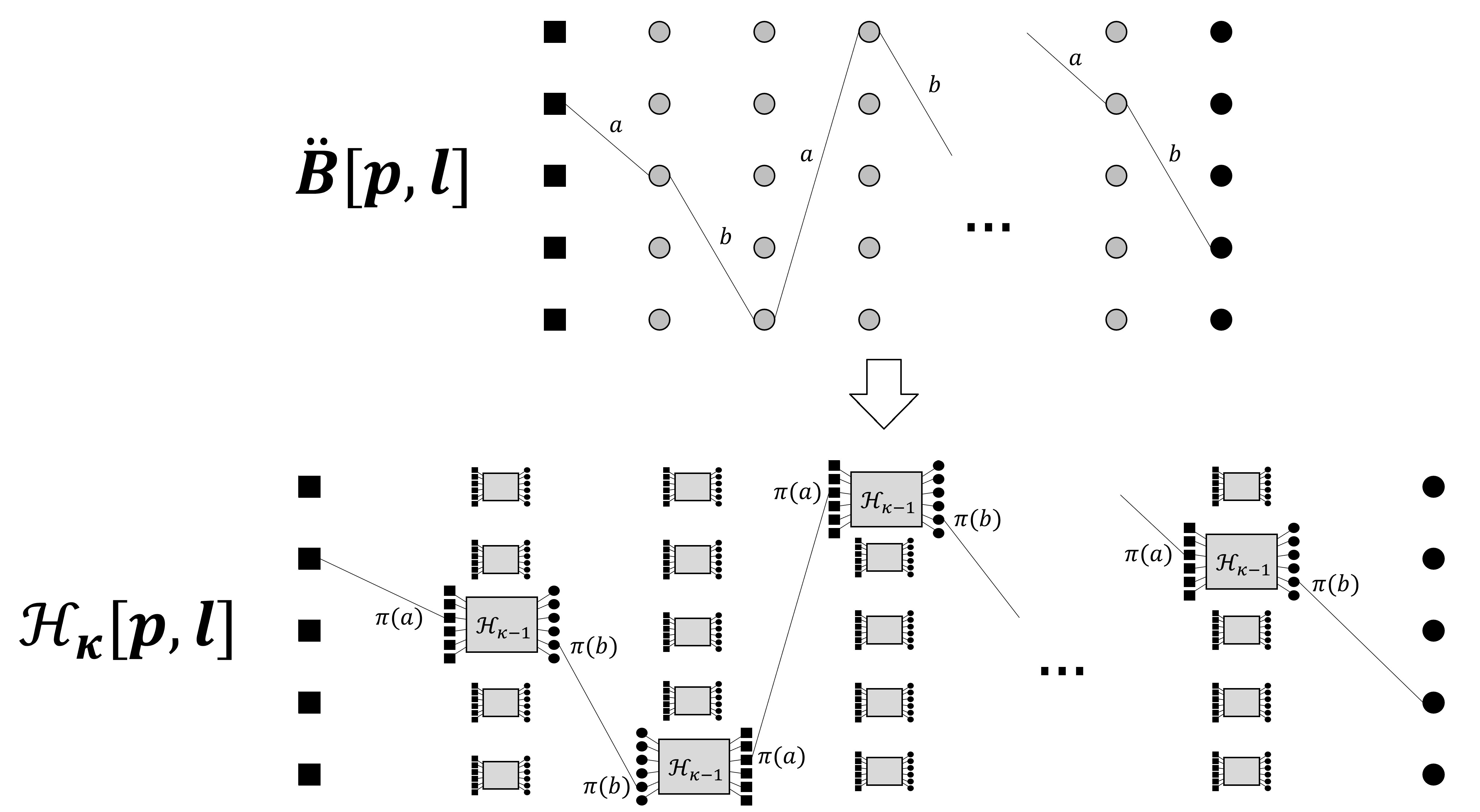
The graph is the same graph as , where every vertex in its middle layers is replaced by a copy of the complete bipartite graph , where is the number of labels in (for , these vertices are replaced by copies of ). Each vertex in each side of the copy of is mapped to a label in . An original edge of , that had label , now connects these copies of , by their vertices that correspond to the label (see Figure 1 in Section 3.1 for a detailed illustration). In addition, these edges are assigned with a large weight of (for , this weight is ). This means that any shortest path in between a pair now must pass through copies of . Other paths that connect , on the other hand, must visit a layer more than once, and therefore their weight is larger than by at least . Choosing (for , ), this means that paths other than the unique shortest path have stretch more then . Hence, any -pairwise -spanner must contain the unique shortest paths between any pair .
In our proof of a lower bound for pairwise spanners, we utilize an additional property of the graph . Recall that the edges of (a shortest path in that connects some ) are alternately labeled by a unique pair of labels . This means that in , shortest paths that connect different pairs cannot share an edge of a copy of . This is due to the fact that if such path goes through the edge of a copy of , and corresponds to a label , and to a label , then it uniquely determines the pair of labels of the path . The result is that any -pairwise -spanner for must contain a disjoint set of edges, for every . Hence, its size must be at least
For larger ’s, the number of the edges that these paths do not share grows to , therefore the lower bound for the size is , where is the corresponding set of pairs of the graph . It can be proved that the number of pairs in is approximately , where is the number of vertices in .
1.3.2 Lower Bound for Pairwise Spanners with Large Stretch
Our proof of a lower bound for pairwise spanners with stretch larger than (typically a constant stretch, or stretch between and , where is such that ) is demonstrated on an unweighted graph with high number of edges and high girth (the length of the minimal cycle). This kind of graphs was used in [31, 26] to show lower bounds for spanners, distance oracles and hopsets. Specifically, we use a graph from [23], that is regular, has edges, and has girth larger than .
Given a desired stretch , we consider pairs of vertices in of distance , henceforth -pairs. The useful property of -pairs is that due to the high girth of , they have a unique shortest path that connects them, while any other path must have stretch more that . Note the similarity of this property to the property of the unique shortest paths from the lower bound for near-exact pairwise spanners. This property implies that any -pairwise -spanner, for any set of -pairs, must contain all the unique shortest paths that connect the -pairs of . We call such paths the -paths that correspond to the -pairs in .
Then, we use the regularity of the graph , as well as the high girth of , to prove some combinatorial properties of . We prove that there are many -pairs - approximately pairs - and that each edge participates in a large number of corresponding -paths - approximately .
To finally prove our lower bound for pairwise -spanners, we sample a set of -pairs out of all the possible such pairs. This means that the sample probability is . But since the number of -pairs whose corresponding -path pass through a specific edge is approximately , we expect that a constant fraction of the edges of still participate in a unique shortest path of the -pairs in . Every -pairwise -spanner must contain these edges, and therefore must have size
This proves our lower bound of .
1.3.3 Upper Bound for Pairwise Spanners with Large Stretch
The state-of-the-art pairwise -spanners and pairwise -spanners of [19] were achieved using the following semi-reduction from hopsets. Suppose that the hopset has stretch and hopbound , for a graph . Given a set of pairs of vertices , we construct a pairwise spanner that consists of all the -edges paths in that connect pairs in and have stretch . Of course, these paths include edges of that are not allowed to be on the final pairwise spanner (as they don’t exist in ). Therefore, an additional step is required, that adds more edges to , such that every edge will have a path in with weight . This way, the distance between every pair is the same distance as in the graph , which is at most . The size of the pairwise spanner is , plus the number of edges that are required to preserve the distances between every .
In [19], preserving the distances between pairs in is done by relying on the specific properties of the hopset . Namely, it was observed that the relevant hopset has small supporting size - the minimal number of edges required to preserve the distances in . We, however, take an alternative approach. Instead of relying on specific properties of the hopset to preserve it accurately, we use a pairwise spanner with low stretch, to preserve the distance in approximately. In fact, we use the very same -pairwise -spanner of [19] to do that.
Considering the process described above, we are only left to choose the hopset that we use, to achieve a pairwise spanner with relatively large stretch. The advantage of having a large stretch , is that the hopbound can be much smaller, and as a result, so is the size overhead of the resulting pairwise spanner. In particular, for pairwise -spanners, we know by Section 3.1 that the size overhead must be . But for a larger stretch , we can get a much smaller hopbound, and therefore a much smaller size overhead, of . This is done by using the state-of-the-art hopsets with this type of stretch, from [5, 26].
However, the process of directly applying a pairwise spanner with low stretch on a hopset described above, results in a somewhat large size of the pairwise spanner. This is because the size of the hopset, which is roughly , is multiplied by the size overhead coefficient , which is at least . To reduce this size, and avoid the additional term of , we eventually do use certain properties of the hopsets of [26]. Specifically, we prove that their hopsets could be partitioned into three sets , such that can be efficiently preserved, while is relatively small. Thus, we can use a pairwise spanner with low stretch only on , instead of using it on the whole hopset . Then, the coefficient multiplies only the size of , which is significantly smaller than .
1.3.4 Subset, Source-wise and Prioritized Spanners
Our new results for subset, source-wise and prioritized spanners are achieved via a series of reductions. These reductions implicitly appeared in [19, 10]. The first reduction receives a pairwise spanner and uses it in order to construct a subset spanner. A subset spanner is a special type of pairwise spanner, for which for some . The second is a quite simple reduction that turns a subset spanner into a source-wise spanner with almost the same properties. The last reduction uses source-wise spanners to construct prioritized spanners. Using the new state-of-the-art pairwise spanners, we achieve new results for each of these types of spanners.
Besides these new results, we believe that these reductions themselves could be of interest. It is immediate to find backwards reductions, from prioritized spanners to source-wise spanners, and from source-wise spanners to subset spanners. This means that, in a sense, these three111111Note that the reduction that constructs a subset spanner, given a pairwise spanner, remains a one-way reduction, in the sense that no efficient reduction in the other direction is known. types of spanners are equivalently hard to construct. Every new construction of one of these spanners immediately implies new constructions for the others.
Next we shortly describe the three reductions mentioned above.
From pairwise to subset spanners. Let be an undirected weighted -vertex graph, and let be a subset, for which we want to construct a subset spanner. We consider the graph , where every pair of vertices is connected by an edge of weight . On the graph , we apply a known construction of emulator (see Definition 4). That is, we find a small graph , such that
for any . The parameter is the stretch of the emulator . For this purpose, we use either the distance oracle of Thorup and Zwick from [31], which can be thought of as an emulator with stretch and size , or the emulator from [19], that has stretch and size . Here, is a positive integer parameter for our choice. These two emulators are path-reporting, meaning that given , they can also efficiently report a path of stretch inside the emulator itself.
Next, we consider the set as a set of pairs of vertices from , and apply a pairwise spanner on this set. We use the existing pairwise spanners from [19] that have stretch either or , and size121212In [19], the size of these pairwise spanners was presented as , where , or , and is the set of pairs. We choose here since for small enough , this is the most sparse that these spanners can get. In our case, the set is the emulator , which is indeed small enough.
Here, when , and when (there is also additional dependency on in the size of the pairwise spanner, in case that ). These two pairwise spanners are also path-reporting.
Now fix a pair of vertices . In the graph , the shortest path between is the single edge , that has weight , and thus in there is a path between that has weight . Note that this path consists of edges of , which are not actual edges of the graph . For that reason, we use our pairwise spanner, to find, for every edge on this path, a path in that replaces and has weight of at most . The result is a path in , with stretch . That is, the resulting spanner has a -stretch path for every pair of vertices in . Hence, this is a subset spanner. Note that since both the emulator and the pairwise spanner we used were path-reporting, then so is the resulting subset spanner.
From subset to source-wise spanner. Let be an undirected weighted graph, and let be a subset. Suppose that is an -subset spanner with stretch . To construct a source-wise spanner for , we just add to a shortest path, from every vertex to its closest vertex in . If the shortest paths and the vertices are chosen in a consistent manner, it is not hard to prove that the added edges form a forest. Thus, the increase in the size of the spanner is by at most edges, and also we can easily navigate from a vertex to the corresponding (we simply go towards the root of ’s tree).
Given any and , the spanner contains the shortest path, concatenated with the path in from to . It can be shown that it has at most stretch. Also, if the subset spanner is path-reporting, then so is the new source-wise spanner.
From source-wise to prioritized spanner. In the setting of prioritized spanners, we get a priority ranking of the vertices of : . To construct a prioritized spanner based on source-wise spanners, we consider a sequence of non-decreasing prefixes of this list:
where is some non-decreasing function, and we apply a source-wise spanner on each of them. The idea is that in the construction of the source-wise spanners for the first prefixes in the list, we may use a smaller stretch. Then, since these prefixes are small enough, the size of the resulting source-wise spanners will not be too large.
Specifically, our path-reporting prioritized spanner with size is achieved by using a sequence of prefixes of sizes . Recall that the size of an -source-wise spanner with stretch is , where . Note that for , by choosing , the first term is . Thus, we must choose a bit larger than , in order to obtain an -source-wise spanner with size (this is the sparsest -source-wise spanner we can obtain, since our pairwise/subset/source-wise spanners always have an additive term of in their size). Namely, for cancelling the factor , we must choose .
In the choice of above, the factor in the denominator is actually . This means that we cannot make this choice for prefixes with . For this reason, we cannot choose such that the prefixes will cover the entire priority ranking , or most of it (to cover vertices, we need ). Instead, we choose to be roughly . The size of the resulting prioritized spanner is , and the covered vertices are the vertices such that . For queries that include a covered vertex , the stretch is roughly , where is the minimal integer such that . That is, the stretch is approximately .
For uncovered vertices (i.e., vertices such that ), we simply add a (non-prioritized) spanner, that has stretch for all the vertices of . The size of such spanner may be as low as , using results from [19]. This spanner, as well as all the source-wise spanners we used, are path-reporting, therefore the resulting prioritized spanner is also path-reporting.
We provide another variation of a path-reporting prioritized spanner with reduced stretch, at the cost of increasing the size to . To achieve that, we change the sequence of prefixes we use, to a sequence of prefixes with sizes . This sequence grows slower than the previous one. While increasing the size of the resulting prioritized spanner, this enable us to control the stretch of each source-wise spanner more carefully.
1.4 Organization
After some preliminaries in Section 2, we prove our new lower bounds for pairwise spanners in Section 3 (lower bounds for pairwise spanners with stretch are in Section 3.1, while Section 3.2 is for higher stretch). For the high stretch regime, we prove our new upper bounds for pairwise spanners in Section 4. Lastly, in Section 5 we show the reductions between pairwise, subset, source-wise and prioritized spanners, which result in new upper bounds for these types of spanners. Appendix A provides missing proofs for Section 4.
2 Preliminaries
Given an undirected weighted graph , we denote by the distance between the two vertices . When the graph is clear from the context, we sometimes omit the subscript and write .
When the given graph is weighted, denotes the weight of the edge . For every set of edges (e.g., a tree or a path), we denote . If is a path, we denote by the length of , i.e., the number of its edges.
2.1 Path-Reporting Pairwise Spanners
In this paper we provide pairwise spanners with the additional property of being path-reporting.
Definition 1 (Path-Reporting Pairwise Spanner).
Let be an undirected weighted graph, and let be a set of pairs of vertices in . A path-reporting -pairwise -spanner for , with query time , is a pair , where is a subgraph of , and is an oracle (a data structure), that given a pair , returns a path in , within time , such that
The size of a path-reporting pairwise spanner is defined as . Here, is the set of edges in , and is the storage size of the oracle , measured in words.
The subgraph is called a pairwise spanner of . A path-reporting preserver is a path-reporting pairwise -spanner.
Remark 1.
Note that in path-reporting pairwise spanners (and also in path-reporting emulators, which will be defined later), a query that outputs a path always has query time . This is inevitable, because a part of the task of a query is to report the path itself. A standard approach in the area of path-reporting structures (see [18, 27, 19]) is to measure, instead of the whole query time, only the additional query time besides reporting the path. More specifically, if the running time of each query of a path-reporting spanner/emulator is , where is the output path of the query, we say that this path-reporting spanner/emulator has query time .
In [19], two path-reporting pairwise spanners were presented, one of them with stretch (a near-exact pairwise spanner), and one of them with stretch . We state these results again here, so we can use them later in Section 5.
Theorem 1 ([19]).
Given an undirected weighted -vertex graph , an integer , a positive parameter , and a set of pairs , there is a -pairwise -spanner for with size
where .
Theorem 2 ([19]).
Given an undirected weighted -vertex graph , an integer , a positive parameter , and a set of pairs , there is a -pairwise -spanner for with size
where .
2.2 Other Types of Path-Reporting Spanners
Besides pairwise spanners, there are several special types of spanners, which we define below.
Definition 2.
Let be an undirected weighted graph, and let be a subset of its vertices.
-
•
A path-reporting -spanner for is a path-reporting -pairwise -spanner, where .
-
•
A path-reporting -subset -spanner for is a path-reporting -pairwise -spanner, where .
-
•
A path-reporting -source-wise -spanner for is a path-reporting -pairwise -spanner, where .
The subgraph is called a spanner, a subset spanner, or a source-wise spanner, respectively.
Definition 3 (Path-Reporting Prioritized Spanner).
Let be an undirected weighted graph, and fix a permutation of . This permutation is called a priority ranking of . A path-reporting prioritized spanner for , with prioritized stretch and prioritized query time , is a pair , where is a subgraph of , and is an oracle that given a query such that , returns a path in with weight at most , within time at most . The size of is defined as , where is the set of edges in , and is the space required to store . The subgraph is called a prioritized spanner.
A result of [19] was the construction of several path-reporting spanners (referred as interactive spanners in [19]) with smaller size, stretch and query time than what was known before. We state here two of these results.
Theorem 3 (Theorem 6 in [19]).
For every undirected weighted -vertex graph and parameters such that and , there is a path-reporting spanner with stretch , query time and size
Theorem 4 ([19]).
For every undirected weighted -vertex graph and parameter such that , there is a path-reporting spanner with stretch , query time and size
2.3 Path-Reporting Emulators
A key component of our constructions in Section 5 is the use of path-reporting emulators.
Definition 4.
Let be an undirected weighted graph. A path-reporting -emulator for is a pair , where is a weighted graph with weights , and is an oracle (a data structure), that given , returns a path in , such that
The graph is called an -emulator. The parameter is called the stretch of the path-reporting emulator . We say that the query time of is if the running time of the oracle on a single query is , where is the output path. The size of is defined as , where is the storage size of the oracle , measured in words.
The distance oracle of from [31] can be viewed as a path-reporting emulator. Considering the improvement to its query time by [33], it can be summarized in the following theorem.
Theorem 5 ([31, 33]).
For every undirected weighted -vertex graph and integer , there is a path-reporting -emulator for with query time and size .
In [19], the authors introduced another path-reporting emulator, that had reduced size and query time, with respect to that of Theorem 5, while its stretch was larger by a constant factor. This emulator is based on the distance oracle of [24].
Theorem 6 ([19]).
For every undirected weighted -vertex graph and integer , there is a path-reporting -emulator for with query time and size .
3 Lower Bounds for Pairwise Spanners
3.1 Near-exact Pairwise Spanners
To prove our lower bound for pairwise -spanners, we use almost the same construction of a graph as the one appears in [2]. Our argument that achieves this lower bound, however, is somewhat different. Before we go into the specific details of the construction, we overview the properties of the graph of [2].
The authors of [2] constructed a sequence of graphs , each with a layered structure. The first and last layers of serves as input and output ports (respectively), while the interior layers are made out of many copies of . Then a relatively large set of input-output pairs is defined, such that for every there is a unique shortest path in between , that passes through each layer exactly once. The edges between the layers of are heavy enough, such that any other path from to suffers a large stretch, since it must visit at least two layers more than once (in the unweighted version, the edges between the layers are replaced with long paths).
We now construct a sequence with the same properties. The construction is essentially the same as in [2]. However, we fully describe it in details here, because (1) there are slight differences from the original construction, and (2) our lower bound proof refers to the specific details of this graph and the way it was constructed. We do use the second base graph from Section 2.2 in [2] as it is (this graph is actually originated in [1]).
The second base graph is an undirected unweighted graph, denoted by , where are two positive integer parameters. The vertices of this graph are organized in layers, each of them with size , such that all the edges of the graph are between adjacent layers. The vertices on the first layer of are called input ports, and the vertices on the last layer of are called output ports. Aside from the graph itself, there is a set of pairs of input-output ports , such that every pair in this set is connected in by a unique shortest path. The size of is , thus it contains a large portion of all the possible input-output pairs. Lastly, the graph has labels on its edges, such that the edges on the unique shortest path of every input-output pair in are labeled alternately by two labels. One can think of these labels as routing directions to get from an input to an output.
Formally, the graph is described in the following lemma. The proof of this lemma is implicit in [2], in which the construction of the graph is described.
Lemma 1.
Let be two integer parameters. There is a function which is non-decreasing in the parameter , and there is an undirected unweighted graph , with the following properties.
-
1.
The vertices of the graph are partitioned into disjoint layers , each of them of size , such that every edge of is between vertices that belongs to adjacent layers.
-
2.
There is a set of edge-labels of size , such that for every , every vertex , and every label , there is exactly one edge from to a vertex , that is labeled by (the vertex is different for every label ).
-
3.
Given a vertex and a pair of labels , let be the path that starts at , and its edges are labeled alternately by the labels (starting by ). Here, is the vertex in which the path ends, and we denote . Then, is the unique shortest path in . Moreover, for any other , the path , that is alternately labeled by the same labels and ends in , is vertex-disjoint from .
The specific details of the construction of the graph appear in [2]. We, however, only use the properties that are described in Lemma 1, and do not need these details for our proof. We now define the sequence of graphs recursively, where are any two integer parameters. For every , we also define a corresponding set of pairs of vertices from .
The graph is defined to be the complete bipartite graph . The corresponding set of pairs is defined to be all the pairs , of a vertex from the left side of and a vertex from its right side.
To construct for , we start with the graph from Lemma 1. The vertices of this graph are partitioned into layers , where edges only exist in between adjacent layers. We call the vertices in the first layer input ports, and the vertices in the last layer output ports. The rest of the vertices of are called internal vertices. The input and output ports also serves as the input/output ports of the graph (in particular, there are input ports and output ports in ). Let be the set of edge-labels, as described in Lemma 1, and let be the corresponding set of pairs from Definition 2. Let . We fix an arbitrary bijection .
Consider the graph . Using , we match each input/output port of this graph to a label in . We replace each internal vertex of by a copy of the graph . For a vertex in , denote this copy by . Let be an edge in with label , such that , . In , we replace this edge by an edge of weight as follows.
-
•
If is even, the new edge is added from the -th input port of (or, in case that , from itself) to the -th input port of .
-
•
If is odd, the new edge is added from the -th output port of to the -th output port of (or, in case that , to itself).
In other words, we can imagine that the copies of are inserted as they are in odd layers, and reversed in even layers. This way, input ports are connected to input ports, and output ports are connected to output ports. See Figure 1 for an illustration.
This completes the description of the graph . We define the corresponding set as follows. Given some , let be the unique pair of labels such that the shortest path in is labeled alternately with . Henceforth, we call the corresponding labels to . Denote by the -th input port of , and by the -th output port of . We say that if and only if .
The following lemma is our version of Lemma 2.2 from [2]. We prove it here since our construction of is slightly different.
Lemma 2.
Proof.
We prove the lemma by induction on . For , by definition
Fix , and fix an input port of . Denote by the set of pairs , i.e., the set of pairs in with as their input port. We show a bijection between the sets and . Let be a pair in , and let be the corresponding labels to . By the definition of , the -th input port and the -th output port of satisfy . Thus, we map the pair to the pair .
To prove that this mapping is a bijection, we now show the inverse mapping. Note that for any , there are unique labels such that is the -th input port and is the -th output port of . This is true since is a bijection. Let be the output port of , such that (using the notation from Lemma 1). Then, are the corresponding labels to , and since , we conclude that . That is, .
The two mappings that were described in the two paragraphs above are the inverse of each other, hence our mapping is a bijection, and we conclude that . Summing over all the input ports of , and using the induction hypothesis, we get
By Lemma 1, we know that , and that , since is a non-decreasing function in the first variable (and ). Hence,
∎
Next, we estimate the number of vertices in . Denote this number by .
Lemma 3.
For every ,
Proof.
We again prove the lemma by induction on . For , the graph is the complete bipartite graph . Therefore,
For , recall that was obtained by replacing each of the vertices in the interior layers of , by a copy of . The number of vertices in any of these copies is
On the other hand, this number is also
In these bounds we used the induction hypothesis, the fact that is a non-decreasing function, and the bounds on from Lemma 1.
We conclude that the number of vertices in is
and also
This completes the inductive proof.
∎
In [2], the authors showed that any -spanner for this graph131313For the lower bound for near-additive spanners, one need to use an unweighted graph. Thus, [2] actually used a similar graph where the edges between the copies of are replaced by paths of length . This graph has essentially the same properties as the graph described here., that has less than edges, must have . But note that by Lemma 3, the number of vertices in is , while Lemma 2 proves that the number of pairs in is roughly
Thus, the result of [2] means that less than edges in a near-additive spanner implies .
In our case, we will show that any -pairwise -spanner for must have at least edges, for . Otherwise, the stretch guarantee will not hold for at least one of the pairs in .
To achieve this goal, we prove some properties of the shortest paths that connect the pairs in . A key notion will be that of a critical edge, which also appears in [2].
Definition 5.
An edge of is said to be critical if it lies in a copy of .
The following lemma is parallel to Lemma 2.3 in [2].
Lemma 4.
The distance between any input and output port of is at least .
Moreover, for every pair , there is a unique shortest path in that connects , and has weight . This path does not share a critical edge with any other shortest path , for . That is, there are no critical edges in , for any pair in .
Proof.
We prove the Lemma by induction over . For , the graph is the complete bipartite graph . One of its sides consists of the input ports, and the other consists of the output ports. Thus, the distance between any input port and output port is at least . For every , the edge is clearly the unique shortest path between that has weight . In addition, this path does not share its only critical edge with any other shortest path in , for .
Fix . Every path that starts from an input port of and ends in an output port must visit at least copies of , each one of them replaces a vertex from a different layer of . By the induction hypothesis, passing through a copy of , from an input port to an output port (or vice versa), requires a path of weight at least . The edges that connect the different copies are of weight . Note that any path from the input layer of to its output layer must pass through at least of these edges. Overall, such path must have weight of at least
Now fix a pair . Recall that by definition, we know in particular that are vertices of , and . By Lemma 1, in the graph there is a unique shortest path , labeled by some two labels . Denote by the copies of that replaced the vertices in the construction of .
Recall that by its construction, the graph contains the following edges. For every even , it contains an edge of weight from the -th input port of (or from itself if ) to the -th input port of . For every odd , it contains an edge of weight from the -th output port of to the -th output port of (or to itself if ). Also, recall that since , it means that (here, and in the rest of this proof, we identify with the -th input port and -output port of ). Thus, when using the edges described above, we can also find paths inside the copies , each of them with weight . We conclude that there is a path in with weight
Denote this path by . Since we already proved that the distance between any input port and any output port is at least , we deduce that is a shortest path between .
Let be a different path than between and in . Consider the list of copies of that passes through, by the same order they appear on . Since , there are two cases: either this list is identical to , but for at least one the path passes through using a different path than , or this list is not identical to .
In the first case, by the induction hypothesis, the path that uses inside has weight strictly larger than . The path inside the other copies has weight of at least , again by the induction hypothesis. Together with the edges with weight that connect these copies, we get that the weight of is strictly more than
In the second case, we ”translate” the path into a path in , by replacing each copy of it passes through by the corresponding vertex of . The path is different from the path . Since the latter is the unique shortest path in , the path must pass through a layer of more than once (otherwise its weight would be equal to the weight of ). That is, passes through at least internal vertices of and contains at least edges. This means that the path contains at least edges of weight . Also, note that (like any other input-output path in ) must pass through at least copies of . By the induction hypothesis, the weight of is at least
In conclusion, the path has length , while any other path in has a larger weight. Thus, is a unique shortest path between in .
To complete the proof, we have to show that if and share a critical edge, for some , then it must be that . Let be such two pairs. Since their paths share a critical edge, they must pass through the same copy of . Denote this copy by . We saw that the path is originated in a path in the graph , which is the unique shortest path between that satisfies , and that the edges of are alternately labeled by some . Moreover, , because (recall that we still identify the numbers with input and output ports of ). Symmetrically, the path and the labels that correspond to the path in satisfy . Note that the unique shortest paths between and between still share a critical edge. Thus, by the induction hypothesis, , or equivalently .
Notice that the two paths pass through the same vertex in , because pass through the same copy . We also know that they are alternately labeled by the same to labels . By Lemma 1, it must be that , and in particular , otherwise they cannot have the same pair of labels . This completes the inductive proof.
∎
We are now ready to prove our main theorem.
Theorem 7.
For infinitely many integers , and for any integer and real , there is an -vertex graph and a set of pairs with size at least , such that any -pairwise -spanner for must have at least edges, where .
Proof.
Fix and . Let be , for and some arbitrary . Denote . We will show that any -pairwise -spanner for must have size of at least . This proves the theorem for
For the size of , recall that the number of vertices in is , by Lemma 3. Thus,
Therefore, by Lemma 2, the size of is at least
Here we used Lemma 1 to bound , we used the fact that , and we used the fact that (this is trivial, by the construction of ).
Let be a subset of the edges of , with . By Lemma 4, for every pair , the unique shortest path in has a disjoint set of critical edges that it goes through. Therefore, there must be some such that contains less than of its critical edges.
We prove by induction on that in the graph , if a pair has less than of its critical edges in , then
For , a pair that has less than of its critical edges in , means a pair such that . Since the graph is bipartite, .
Fix , and let be a shortest path in , for a pair that has less than of its critical edges in . Consider the path in that is obtained by replacing each copy of that passes through by the corresponding vertex of . If is not the unique shortest path between in , then the path must pass through a layer of more than once (otherwise its weight would be equal to the weight of ). That is, passes through at least internal vertices of and contains at least edges. This means that the path contains at least of weight . Note that must pass through at least copies of , just to get from to . By Lemma 4, the weight of is at least
If the path equals to , the unique shortest path in , then it passes through exactly internal vertices of . Hence, passes through exactly of copies of . We would like to know how many of them contain less than critical edges of . Note that there cannot be less than such copies: otherwise the number of copies with at least critical edges of is more than , i.e., at least , so there are at least critical edges of in , in contradiction. Therefore, the number of copies in which there are less than critical edges of is at least . In these copies, suffers a weight of at least , by the induction hypothesis. In the other copies, must have a weight of at least , by Lemma 4. Together with the edges that connect these copies and have weight of , we get
This completes the inductive proof. It shows that there is a pair with
Where in the last step we used the definition of . Thus, cannot be a -pairwise -spanner. In other words, any -pairwise -spanner must have size of at least , where .
∎
Remark 2.
Notice that the proof of Theorem 7 also works for every subset of the pairs . Therefore, the phrasing of Theorem 7 may be strengthen as follows.
For infinitely many integers , and for any integer and real , there is an -vertex graph and a number , such that for every integer , there is a set of pairs with size , such that any -pairwise -spanner for must have at least edges, where .
3.2 Large Stretch
The lower bound for pairwise spanners with large stretch is achieved using a graph with high girth and large number of edges. This properties of a graph were used for proving lower bounds for distance oracles and spanners (see [31]) and also for hopsets (see [26]). In particular, we use the same graph that was used in [26], which was introduced by Lubotzky, Phillips and Sarnak in [23]. This graph has the additional convenient property of being regular, besides its high girth and large number of edges. Its exact properties are described in the following theorem.
Theorem 8 ([23]).
For infinitely many integers , and for every integer , there exists a -regular graph with and girth at least , where , for some universal constant .
Fix such that , and a large enough as in Theorem 8. Let be the corresponding -regular graph from Theorem 8. The girth of is at least , thus larger than . Denote . Define the following set of pairs .
Lemma 5.
For every , there is a unique shortest path between in . Furthermore, for every tour between , that has length , we have .
Proof.
Let be some shortest path in , and let be a tour with . If , then the union contains a cycle. This cycle is of length at most
by the definition of . This is a contradiction to the fact that the girth of is larger than . Hence, . In case is also a shortest path, i.e., , then implies . That is, is the unique shortest path between in .
∎
Henceforth, we use the notations from Lemma 5, that is, we denote by the shortest path in .
Lemma 6.
Let be some subset, and suppose that is a -pairwise -spanner for . Then,
Proof.
Fix some . Since has stretch for every pair in , we know that there is a path with . By Lemma 5, the shortest path satisfies . In conclusion, for every , thus .
∎
The following lemma describes several combinatorial properties of the graph .
Lemma 7.
The number of edges in is . The number of paths in is . For every edge , there are pairs such that .
Proof.
The number of edges is half the sum of the degrees in . Since is -regular, we get .
Now fix some , and consider its BFS tree up to distance . The root has children in this tree, and every other internal vertex has a set of children, disjoint from the children set of any other vertex in this tree. This is true since otherwise there would be a cycle of length at most , in contradiction to the girth of being larger than . Thus, the number of vertices in the -th layer of this tree, is . That is, the number of such that is . Hence,
In this sum, each pair is counted exactly twice, therefore .
The proof of the third property is very similar. Fix some edge . For every integer , consider the BFS tree of up to distance . Symmetrically, denotes the BFS tree of up to distance . As before, the children sets of the vertices in are disjoint - otherwise there would be a cycle of length at most
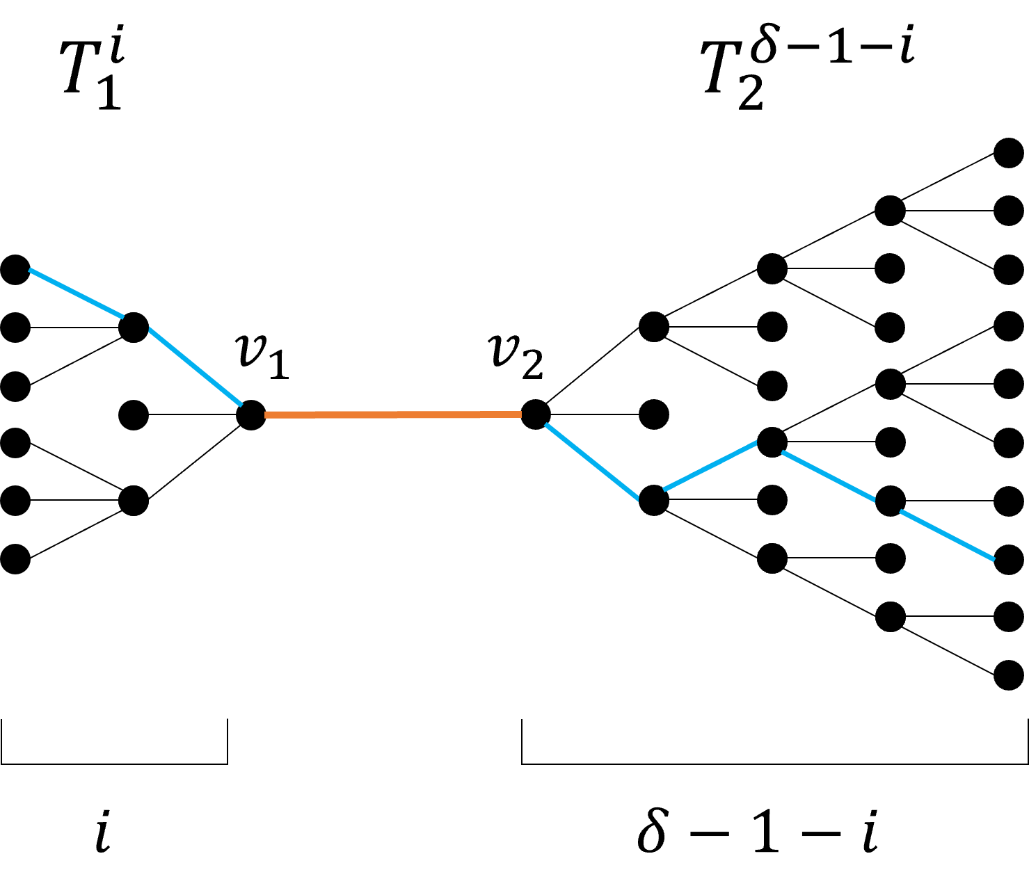
in contradiction. Hence, the number of vertices in the -th layer of is (note that has children in this tree), and the number of vertices in the -th layer of is . For every pair such that , the path has one end in the -th layer of and the other end in the -th layer of , for some . See Figure 2 for an illustration. Thus, the number of such pairs is
∎
We are now ready for the main theorem of this section.
Theorem 9.
For infinitely many integers , and for any real and integer such that , there is an -vertex graph and a set of pairs with size , such that any -pairwise -spanner for must have at least edges, that is, the size overhead is .
Proof.
By Theorem 8, for infinitely many integers , there is a -regular graph with vertices and girth larger than , where . We use the same notations for and as in the beginning of this section.
Let be a subset that is formed by sampling each pair in independently with probability . The expected number of pairs in is
by Lemma 7. Moreover, by Chernoff bound,
| (3) |
for large enough , where we used the fact that .
We say that a pair covers an edge if . For an edge , the number of pairs in that cover is , by Lemma 7. Therefore, the probability that none of the pairs that cover are in is . Hence, If we denote by the set of edges that are not covered by any , then . By Markov’s inequality,
| (4) |
Now, by the union bound, the probability that either , or , is at most , using Inequalities (3) and (4). Therefore, there is a way to choose the subset , such that the number of edges in that are not covered by any is at most , and such that . In particular,
For this choice of , the number of edges that satisfy for some is at least . Notice that these are exactly the edges in . By Lemma 6, any -pairwise -spanner for must contain this set, and therefore must have size at least
This proves the theorem for .
∎
4 An Upper Bound for Path-Reporting Pairwise Spanners
To construct path-reporting pairwise spanners with relatively large stretch (e.g., pairwise -spanners with ) and small size, we combine hopsets that have large stretch with pairwise spanners that have small stretch. More precisely, suppose that the hopset for an -vertex graph has stretch and hopbound . Recall that for every pair of vertices , there is a path with at most edges, and weight at most . To construct a pairwise spanner for the graph and some pairs set , we first add the edges of , for every , to the desired spanner. Note that for each pair in we added at most edges. Next, we consider as a set of pairs of vertices in , and we use a pairwise spanner with small stretch on . We insert the edges of to our pairwise spanner. The result is a -pairwise spanner for , with stretch at most , and size at most . To make this pairwise spanner path-reporting, we make sure that the pairwise -spanner we used is also path-reporting, and we also store in the oracle the paths for every .
A similar technique, of combining a hopset with a pairwise spanner, appeared in [19]. In [19], however, preserving the edges of the hopset was mostly done by relying on the properties of itself, and claiming that there is a small size exact preserver (i.e., pairwise -spanner) for .
The combination described above, between a hopset and a pairwise spanner with small stretch, is relatively simple. We later show a more complicated construction that achieves better results. This construction relies on specific properties of the hopset we use. Both of these constructions of pairwise spanners with large stretch are also path-reporting.
4.1 Warm Up: Path-Reporting Pairwise Spanners via Hopsets
We start with the relatively simple procedure of constructing a path-reporting pairwise spanner, via a combination of a hopset and a path-reporting pairwise -spanner, for small .
Lemma 8.
Let be an undirected weighted graph on vertices, and let be a hopset for with stretch , hopbound and size . Suppose that for every set of pairs , there is a path-reporting -pairwise -spanner for with query time and size .
Then, for every set of pairs in , there is a path-reporting -pairwise -spanner for , with query time and size
Proof.
For every pair of vertices , there is a path with at most edges, and weight at most . We consider the hopset as a set of pairs in , and conclude that there is a path-reporting -pairwise -spanner for with size at most .
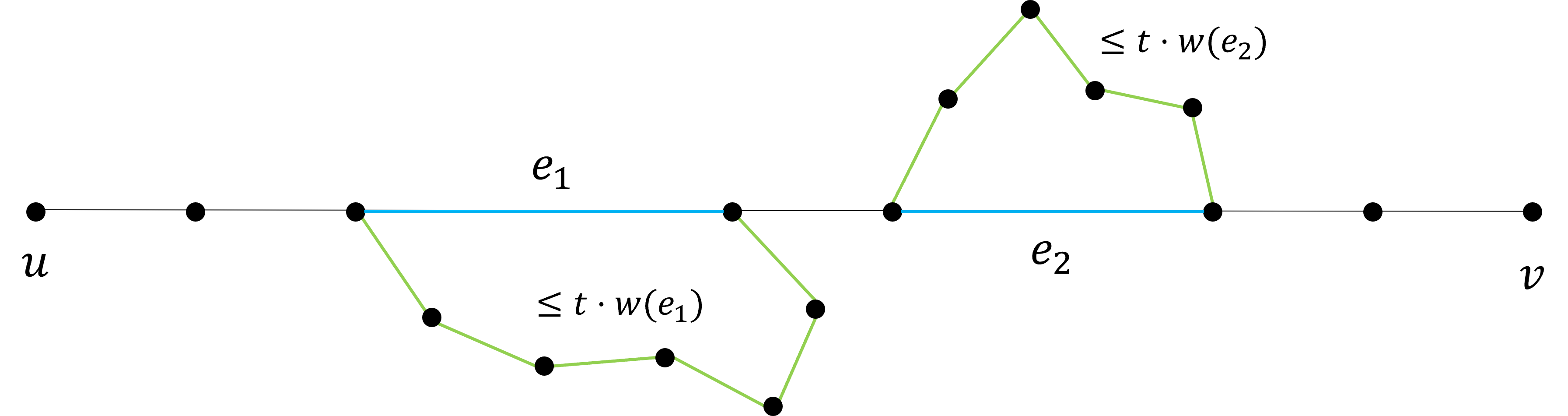
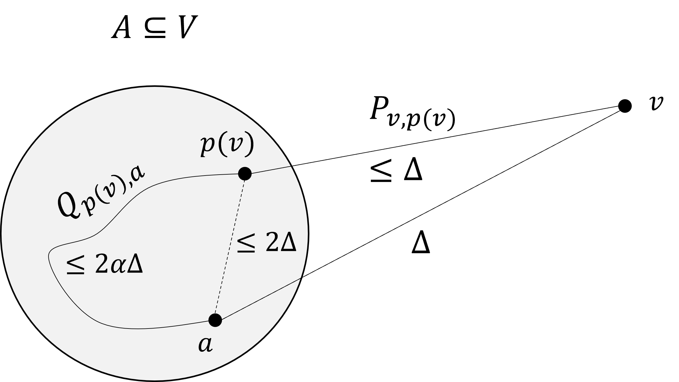
Define a path-reporting pairwise spanner as . In the oracle , we store the oracle and all the paths for every . Given a pair , let be the stored path for . By the hopbound guarantee of the hopset , we know that , and by the stretch guarantee we know that . For every , if , then also , and thus . If , then by the stretch guarantee of the spanner , we have . See Figure 3.
In conclusion, we saw that for every . Hence,
Therefore, the stretch of our pairwise spanner is at most .
The oracle , given a pair , reports the edges of one by one. In case it encounters an edge of , it uses the oracle to replace it with a path in with stretch at most . Notice that this output path is contained in , and by a similar proof as above, it has stretch at most . The running time of this procedure is proportional to the length of the resulting path. Hence, the query time of our pairwise spanner is .
For the size of , we have
The same bound holds for the oracle .
∎
To achieve path-reporting pairwise spanners with large stretch and small size, we use the best known hopsets that have large stretch. These hopsets were presented in [5], and were later reformulated and improved in [26]. Some of the results of [26] can be summarized by the following theorem141414For stretch , [26] provides a hopset with hopbound and size . We focus here, however, on hopsets that have larger stretch and smaller hopbound..
Theorem 10 ([26]).
Let be an undirected weighted graph on vertices, and let be two integer parameters. There is a hopset for with stretch , hopbound , and size .
In addition, we use the state-of-the-art path-reporting pairwise spanner with stretch , from Theorem 2. Lemma 8, when applied with Theorems 10,2, provides the following result.
Theorem 11.
Let be an undirected weighted graph on vertices, and let be a set of pairs of vertices in . For every two integer parameter , there is a path-reporting -pairwise -spanner for , with query time and size
4.2 Path-Reporting Pairwise Spanner with Improved Size
In this section we further improve the size of the path-reporting pairwise spanner from Theorem 11, by decreasing the coefficient of and of . To do that, we first prove an extended version of Theorem 10. In this version, we observe that when considering the hopset from [26] as a set of pairs of vertices, a large part of this set is easy to preserve using shortest paths. That is, for this subset of pairs, there is a path-reporting preserver with small size. For the other pairs, we will use a path-reporting pairwise spanner with small stretch, as we did in Lemma 8.
Theorem 12 (Extended version of Theorem 10).
Let be an undirected weighted graph on vertices, and let be two integer parameters. There is a hopset for with stretch , hopbound , and size .
Moreover, the hopset can be divided into three disjoint subsets , such that has a path-reporting preserver with size , has a path-reporting preserver with size , and
Note that Theorem 12 provides a path-reporting preserver only for , while for , it only bounds the size. The proof of this theorem involves diving into the details of the proof of Theorem 10 from [26]. We bring the full proof in Appendix A.
Given Theorem 12, we use the same scheme as in the proof of Lemma 8 to produce a path-reporting pairwise spanner. This time, we use the path-reporting pairwise spanner from Theorem 2 only on . For , we simply use their path-reporting preserver from Theorem 12.
Theorem 13.
Let be an undirected weighted graph on vertices, and let be a set of pairs of vertices in . For every two integer parameter , there is a path-reporting -pairwise -spanner for with size
Proof.
Let be the hopset from Theorem 12, and let be the corresponding partition of . Let be the path-reporting pairwise spanner from Theorem 2 for the graph and the set of vertices pairs . For , we choose the same parameter as for the hopset . The parameter is chosen as , so that has stretch and size
Let be the path-reporting preservers for . For every pair , let be the path in that has at most edges and stretch at most . We define a path-reporting -pairwise spanner for by
The oracle stores the oracles , and all the paths , for every .
Given a query , the oracle restores the path , and reports its edges one by one. Whenever it encounters an edge of or , it uses the oracle or respectively, to replace this edge with a shortest path, and it reports its edges. For an edges of , it uses the oracle for the same purpose. In this case the resulting path might have stretch at most .
By a similar analysis to the one in Lemma 8, we get a path in that has stretch at most . The time required to report this path is proportional to the length of this output path.
Lastly, we use Theorem 12 to conclude that the size of is at most
In the last step, we used the fact that for every . The size of the oracle has the same bound.
∎
For a constant , we get the following result.
Corollary 1.
For every constant , and , there is a path-reporting -pairwise spanner for , with stretch and with size
Now let , for some . If we set , then we have , and then . By Theorem 13, we get the following result.
Corollary 2.
For every integer and , there is a path-reporting -pairwise spanner for , with stretch and with size
Lastly, for , we get from Theorem 13:
Corollary 3.
For every integer there is a path-reporting -pairwise spanner for , with stretch and with size
5 Subset, Source-wise and Prioritized Spanners
In this section we describe several reductions between the types of path-reporting spanners that were described in Section 2.2. Using these reductions, we obtain a variety of results on these spanners. We start by describing the reductions in a robust way, such that the results themselves will be obtained by substituting specific properties.
5.1 Subset and Source-wise Spanners
The first reduction, from pairwise spanners to subset spanners, also uses a path-reporting emulator (see definition 4). The same reduction appears implicitly in [19].
Lemma 9.
Suppose that every undirected weighted -vertex graph admits a path-reporting -emulator with query time and size . In addition, suppose that any such graph and any set of pairs admit a path-reporting -pairwise -spanner with size .
Then, for every undirected weighted -vertex graph and a subset , there is a path-reporting -subset -spanner with query time and size .
Proof.
Let be an undirected weighted -vertex graph, and let be a subset. Consider the graph with weights on the edges. By our assumption, has a path-reporting -emulator with query time and size . Denote this emulator by and its corresponding oracle by . We consider as a set of pairs by orienting each edge in in an arbitrary direction (alternatively, we may view each edge as two pairs, one in each direction).
The graph and the set of pairs admit a path-reporting -pairwise -spanner with size . Denote this pairwise spanner by and its corresponding oracle by . See Figure 4 for an illustration.
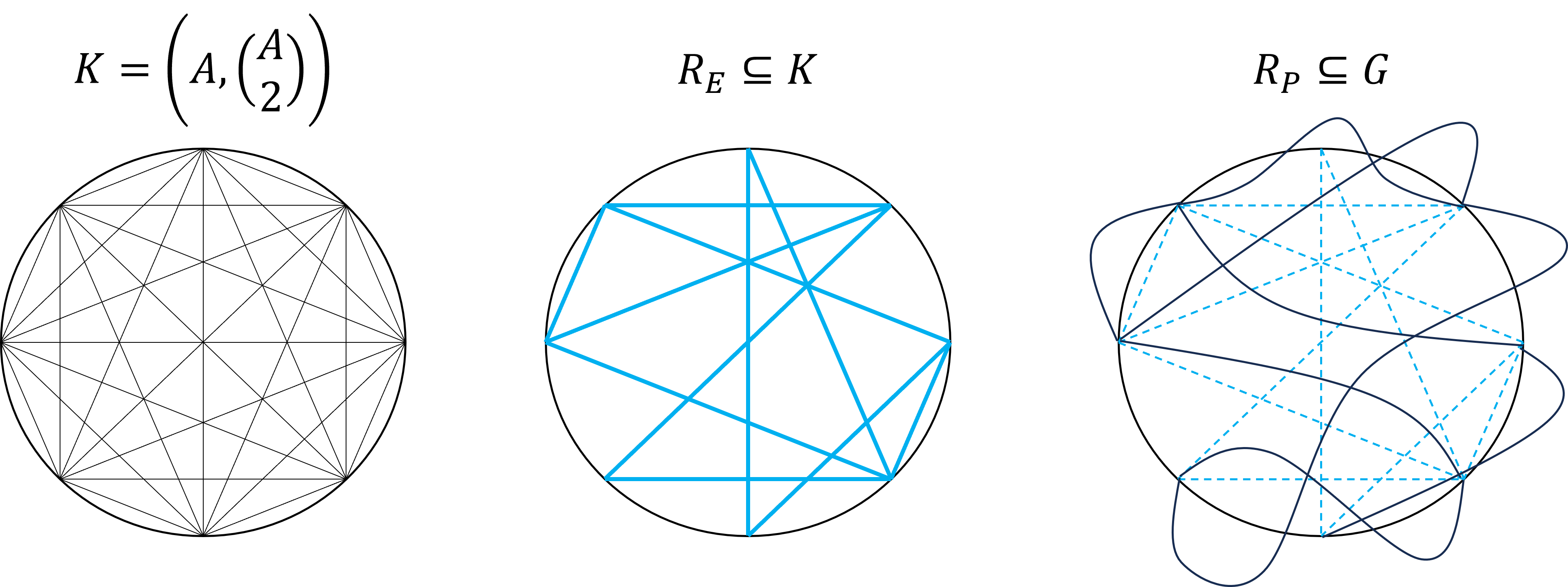
We now define an -subset spanner as follows. The spanner itself is the subgraph of . The corresponding oracle contains the oracles and . Given a pair of vertices , the oracle first finds a path in , with stretch , using the oracle . Then, applies the oracle on every edge of , and concatenates the resulting paths. The result is a tour between in with weight at most , i.e., stretch at most .
The query time of consists of the time required to run a single query of , then query on every edge of the resulting path. The first part is , while each query in the second part runs in time that is proportional to the length of the resulting path. Since concatenates all these paths, this running time is overall proportional to the length of the resulting path, thus we get a query time of .
The size of the oracle is the sum of the sizes of , which is . The size of the spanner itself is . This completes our proof.
∎
Before we apply the reduction from Lemma 9 to get subset spanners, we first show a very simple reduction from subset spanners to source-wise spanners. The resulting source-wise spanner from this reduction has a stretch that is twice as the stretch of the original subset spanner. At the same time, its query time and size are asymptotically the same as in the original subset spanner. This reduction appears implicitly in [10].
Lemma 10.
Suppose that the undirected weighted -vertex graph admits a path-reporting -subset -spanner with query time and size . Then, there is a path-reporting -source-wise -spanner with query time and size .
Proof.
Let be the given path-reporting -subset -spanner. For every vertex , denote by the closest vertex to in the set , breaking ties arbitrarily but consistently. Denote by a shortest path between in . We define a new path-reporting -source-wise spanner as follows.
The set is defined to be the union . The oracle stores the oracle and all the shortest paths , for every , together with a pointer from to the next vertex after on the path . Given a query , the oracle uses the pointers to find the path . Then, it concatenates this path with the path that is returned by . The oracle returns the resulting path as an output.
For the query algorithm to be well-defined, we need to show that indeed can be found using only the pointers . This is true because for every vertex on the path , we have (since if there was a closer -vertex to than , it would be also closer to ). Then, the path is a sub-path of , and the pointer points at the next vertex on this path in the direction to . Hence, the oracle can use these pointers to obtain the path entirely.
The path that outputs is a path in . Note that since is the closest vertex to in , we have . In addition, recall that the stretch of is , thus we have . By the triangle inequality,
We conclude that the weight of the resulting path is
The running time of finding is proportional to the length of itself. Obtaining the path from requires time. Therefore, by our convention of measuring query time for path-reporting spanners, the total query time of the oracle is .
We now bound the size of the path-reporting source-wise spanner . The oracle stores the oracle , which requires size. Aside from , the oracle stores a pointer for every vertex in , thus the size of is . Notice that every edge in the set is of the form , for some vertex . We conclude that the size of is at most .
This completes the proof that is a path-reporting -source-wise -spanner with query time and size .
∎
We now use the reductions from Lemma 9 and Lemma 10 to produce path-reporting subset and source-wise spanners. We apply Lemma 9 on the emulators from Theorems 5 and 6 and on the pairwise spanners from Theorems 1 and 2. The results are given in Theorems 14, 15 and 16.
Theorem 14.
Let be an undirected weighted -vertex graph and let be a subset of vertices. Let be an integer parameter and let be a real parameter. Denote . Then, there is a path-reporting -subset -spanner, with query time and size
Here, , and
In addition, there is a path-reporting -source-wise -spanner, with query time and the same size.
Proof.
Apply Lemma 9 on the path-reporting pairwise spanner from Theorem 1, with parameters instead of , and on the path-reporting emulator from Theorem 5. This provides a path-reporting -subset spanner, with stretch , query time and size151515In the following expression for the size of the subset spanner, appears instead of . This is due to the fact that since the is absorbed by the . Thus, has the same bound as .
| (5) |
If , then . Thus, the third term in (5) is smaller than the first term. If, on the other hand, , then this third term is , which is smaller than the second term in (5). Hence, we get the desired size for the resulting subset spanner.
By Lemma 10, there is also a path-reporting -source-wise spanner with stretch , query time and size
Notice that and therefore
Replacing by in this source-wise spanner gives the desired result.
∎
The size of the subset spanner from Theorem 14 can be improved at the cost of multiplying the stretch by . The proof of the following theorem is identical to the proof of Theorem 14, when using the pairwise spanner from Theorem 2 instead of the one from Theorem 1.
Theorem 15.
Let be an undirected weighted -vertex graph and let be a subset of vertices. Let be an integer parameter and let be a real parameter. Denote . Then, there is a path-reporting -subset -spanner, with query time and size
Here, , and
In addition, there is a path-reporting -source-wise -spanner, with query time and the same size.
Proof.
By Lemma 9, Theorem 2 with parameters instead of , and Theorem 5, there is a path-reporting -subset spanner, with stretch , query time and size
where similarly to the proof of Theorem 15, the third term is smaller from the sum of the first two terms. Here, we replaced by , because , and thus they both have the same bound.
By Lemma 10, there is also a path-reporting -source-wise spanner with stretch , query time and size
Notice that and therefore
Replacing by in this source-wise spanner gives the desired result.
∎
If we allow even larger stretch, the size of the subset spanner further improves. This is achieved by using the path-reporting emulator from Theorem 6, rather then the one from Theorem 5. This also improves the query time of the resulting path-reporting subset spanner.
Theorem 16.
Let be an undirected weighted -vertex graph and let be a subset of vertices. Let be an integer parameter. Denote . Then, there is a path-reporting -subset -spanner, and a path-reporting -source-wise -spanner, both with query time and size
where and
Proof.
Apply Lemma 9 on the path-reporting pairwise spanner from Theorem 2, with parameters , and on the path-reporting emulator from Theorem 6. This provides a path-reporting -subset spanner, with stretch , query time and size
| (6) |
Similarly to the proof of Theorem 14, the third term in (6) is smaller than the first term if , and smaller than the second term if . Hence, we get the desired size for the resulting subset spanner.
By Lemma 10, there is also a path-reporting -source-wise spanner with stretch
, query time and size
∎
5.2 Prioritized Spanners
In this section we describe yet another reduction, that turns our path-reporting source-wise spanners from Section 5.1 into path-reporting prioritized spanners (see Definition 3). This reduction implicitly appears in [10]. In the following lemma, we use the following notation from [26]. Given a function , denote
This notation is well-defined for every , where is the image of , i.e., the set of outputs of the function .
Lemma 11.
Let be an undirected weighted -vertex graph. Suppose that every subset admits a path-reporting -source-wise -spanner with query time and size . In addition, suppose that there is a path-reporting spanner for , with stretch , query time and size .
Then, for every monotonically increasing function , there is a path-reporting prioritized spanner for with prioritized stretch
prioritized query time
and size .
Proof.
Let be the priority ranking of the vertices in . Consider the sequence of monotonically increasing subsets of , where
Let be a path-reporting -source-wise spanner with stretch , query time and size . We define a path-reporting prioritized spanner as follows. Let . The oracle stores all the oracles for , the oracle , and a table of values of the function , for every . Given a query , where , the oracle consider two cases. If , then restores from its table, and apply the oracle on the query . If , then applies the oracle on . The resulting path is the output of .
Fix and let . Recall that is a path-reporting -source-wise spanner with stretch and query time . Note also that by definition, , and therefore . Thus, the prioritized stretch of the oracle on the query , where and , is at most , and the prioritized query time is at most .
For , the stretch and the query time for a query , where , are and respectively.
The storage of the oracle consists of the oracles , for and the oracle . The size of each is and the size of is . Note that the oracle also stores an -sized table for the values of , for every . Hence, the total size of is . The size of the spanner itself is at most . This completes the proof of the lemma.
∎
To use Lemma 11, we need to choose a function , path-reporting source-wise spanners , and a path-reporting spanner . The source-wise spanners we use are from Theorems 14,15 and 16. Note that the size of each of these three source-wise spanners is
where . Here,
We apply Lemma 11 on these source-wise spanners. Every choice of the function yields a path-reporting prioritized spanner with different properties. We now explicitly show the outcomes of several choices of this function. Many other choices that are not presented here can be made, and they might provide prioritized spanners with different properties.
For convenience, in the following theorem we use the notation . That is, is the exponent such that . This notation is useful when comparing our next result with the results of [10]. In [10], non-path-reporting prioritized distance oracles were presented, that had prioritized stretch with size , respectively161616[10] also provided additional non-path-reporting prioritized spanners with sizes and (and possibly could provide many more prioritized spanners with different sizes and stretch parameters). However, as we will see in the proofs of Theorems 17 and 18, our constructions of path-reporting prioritized spanners rely on our source-wise spanners from Section 5.1, that have size . Thus, in this paper we cannot achieve smaller size while keeping the spanners path-reporting.. For comparison, a path-reporting prioritized distance oracle of size was also given in [10], but it had a worse prioritized stretch of .
Theorem 17.
For every undirected weighted -vertex graph , and a real parameter such that , there are path-reporting prioritized spanners with the following trade-offs.
-
1.
size , prioritized stretch
and prioritized query time , where
. -
2.
size , prioritized stretch
and prioritized query time , where
. -
3.
size , prioritized stretch
and query time , where .
Proof.
In what follows, we denote , and . We also denote , and , where is the constant such that the source-wise spanner from Theorem 16 has stretch . We prove the three items in the theorem all at once. To do so, we fix some .
Let be the following function
where . For every , note that if and only if , i.e., . Therefore, we have . In addition, we have
| (7) |
To use Lemma 11 with the function , we first have to specify for every possible subset , which path-reporting source-wise spanner we use. For with size , we use the source-wise spanner from Theorem 14 (for ), Theorem 15 (for ), or Theorem 16 (for ), with
Note that , and in particular , where is the value from these theorems. Then, this source-wise spanner has stretch , query time and size
where in the last step we used the fact that .
For with size , the choice of that we used above is too large, negative or undefined. Thus, in this case we use or any other arbitrary171717Note that in Lemma 11, source-wise spanners of subsets that are larger than are not used. In our case, , and therefore the choice of does not matter in case that . value of .
Lastly, for the role of the path-reporting spanner in Lemma 11, we use the path-reporting spanner from Theorem 3, with . This path-reporting spanner has size
, stretch and query time .
For , we actually use the path-reporting spanner from Theorem 4, with , instead of the one from Theorem 3. This spanner has stretch , query time , and size .
We now apply Lemma 11. Let be a query such that . If - i.e., - then this query has the following stretch in the resulting path-reporting prioritized spanner:
The query time of such query is , when . For , this query time is , since this is the query time of the source-wise spanners from Theorem 16.
For , i.e., for , the query (where ) has stretch and query time , when (these are the same stretch and query time of the path-reporting spanner from Theorem 3). For , such query has stretch and query time (as in Theorem 4, with ).
Finally, we bound the size of the resulting path-reporting prioritized spanner. Here we divide the analysis for the different ’s.
For , note that . Thus, the size of the prioritized spanner is
For , note that . Thus, the size of the prioritized spanner is
For , note that . Thus, the size of the prioritized spanner is
∎
The following theorem improves the size of the prioritized spanners above to , while only slightly increase the stretch (it actually increases it by a factor of at most , with respect to the prioritized spanner from Item 1 in Theorem 17). This time, we use only one of the source-wise spanners from Section 5.1. Using the other two provides similar results.
Theorem 18.
For every undirected weighted -vertex graph , and a real parameter such that , there is a path-reporting prioritized spanner with size , prioritized stretch
and prioritized query time , where
.
Proof.
As in the proof of Theorem 17, we denote . Let be the function
where . For every , note that if and only if , i.e., . Therefore, we have . As a result, we have
| (8) |
We now specify the source-wise spanner that we use for each subset , in order to apply Lemma 11. For with size , we use the source-wise spanner from Theorem 14, with the same as in the proof of Theorem 17:
Note that , and in particular , where is the value from Theorem 14. Then, this source-wise spanner has stretch , query time and size
where in the last step we used the fact that .
For with size , the choice of does not affect the resulting prioritized spanner, thus we choose it arbitrarily.
Lastly, for the role of the path-reporting spanner in Lemma 11, we use the path-reporting spanner from Theorem 3, with . This path-reporting spanner has size
, stretch and query time .
We now apply Lemma 11. Let be a query such that . If - i.e., - then this query has the following stretch in the resulting path-reporting prioritized spanner:
The query time of such query is .
For , i.e., for , the query (where ) has stretch and query time (these are the same stretch and query time of the path-reporting spanner from Theorem 3).
Finally, since , the size of the resulting path-reporting prioritized spanner is
This completes the proof of the theorem. ∎
References
- [1] Amir Abboud and Greg Bodwin. The 4/3 additive spanner exponent is tight. Journal of the ACM (JACM), 64(4):1–20, 2017.
- [2] Amir Abboud, Greg Bodwin, and Seth Pettie. A hierarchy of lower bounds for sublinear additive spanners. SIAM Journal on Computing, 47(6):2203–2236, 2018.
- [3] Reyan Ahmed, Greg Bodwin, Faryad Darabi Sahneh, Stephen Kobourov, and Richard Spence. Weighted additive spanners. In Graph-Theoretic Concepts in Computer Science: 46th International Workshop, WG 2020, Leeds, UK, June 24–26, 2020, Revised Selected Papers 46, pages 401–413. Springer, 2020.
- [4] I. Althöfer, G. Das, D. Dobkin, D. Joseph, and J. Soares. On sparse spanners of weighted graphs. Discrete Comput. Geom., 9:81–100, 1993.
- [5] Uri Ben-Levy and Merav Parter. New (, ) spanners and hopsets. In Proceedings of the Fourteenth Annual ACM-SIAM Symposium on Discrete Algorithms, pages 1695–1714. SIAM, 2020.
- [6] Aaron Bernstein. Fully dynamic (2+ ) approximate all-pairs shortest paths with fast query and close to linear update time. In 2009 50th Annual IEEE Symposium on Foundations of Computer Science, pages 693–702. IEEE, 2009.
- [7] Greg Bodwin. New results on linear size distance preservers. SIAM J. Comput., 50(2):662–673, 2021. doi:10.1137/19M123662X.
- [8] Edith Cohen. Polylog-time and near-linear work approximation scheme for undirected shortest paths. J. ACM, 47(1):132–166, 2000. URL: http://doi.acm.org/10.1145/331605.331610, doi:10.1145/331605.331610.
- [9] D. Coppersmith and M. Elkin. Sparse source-wise and pair-wise distance preservers. In SODA: ACM-SIAM Symposium on Discrete Algorithms, pages 660–669, 2005.
- [10] Michael Elkin, Arnold Filtser, and Ofer Neiman. Prioritized metric structures and embedding. In Proceedings of the forty-seventh annual ACM symposium on Theory of Computing, pages 489–498, 2015.
- [11] Michael Elkin, Arnold Filtser, and Ofer Neiman. Terminal embeddings. Theor. Comput. Sci., 697:1–36, 2017. doi:10.1016/j.tcs.2017.06.021.
- [12] Michael Elkin, Yuval Gitlitz, and Ofer Neiman. Almost shortest paths with near-additive error in weighted graphs. In Artur Czumaj and Qin Xin, editors, 18th Scandinavian Symposium and Workshops on Algorithm Theory, SWAT 2022, June 27-29, 2022, Tórshavn, Faroe Islands, volume 227 of LIPIcs, pages 23:1–23:22. Schloss Dagstuhl - Leibniz-Zentrum für Informatik, 2022. doi:10.4230/LIPIcs.SWAT.2022.23.
- [13] Michael Elkin and Ofer Neiman. Efficient algorithms for constructing very sparse spanners and emulators. ACM Transactions on Algorithms (TALG), 15(1):1–29, 2018.
- [14] Michael Elkin and Ofer Neiman. Hopsets with constant hopbound, and applications to approximate shortest paths. SIAM Journal on Computing, 48(4):1436–1480, 2019.
- [15] Michael Elkin and Ofer Neiman. Linear-size hopsets with small hopbound, and constant-hopbound hopsets in rnc. In The 31st ACM Symposium on Parallelism in Algorithms and Architectures, pages 333–341, 2019.
- [16] Michael Elkin and Ofer Neiman. Centralized, parallel, and distributed multi-source shortest paths via hopsets and rectangular matrix multiplication. In Petra Berenbrink and Benjamin Monmege, editors, 39th International Symposium on Theoretical Aspects of Computer Science, STACS 2022, March 15-18, 2022, Marseille, France (Virtual Conference), volume 219 of LIPIcs, pages 27:1–27:22. Schloss Dagstuhl - Leibniz-Zentrum für Informatik, 2022. doi:10.4230/LIPIcs.STACS.2022.27.
- [17] Michael Elkin and David Peleg. (1+epsilon, beta)-spanner constructions for general graphs. SIAM J. Comput., 33(3):608–631, 2004. URL: http://dx.doi.org/10.1137/S0097539701393384, doi:10.1137/S0097539701393384.
- [18] Michael Elkin and Seth Pettie. A linear-size logarithmic stretch path-reporting distance oracle for general graphs. ACM Trans. Algorithms, 12(4):50:1–50:31, 2016. doi:10.1145/2888397.
- [19] Michael Elkin and Idan Shabat. Path-reporting distance oracles with near-logarithmic stretch and linear size. CoRR, abs/2304.04445, 2023. arXiv:2304.04445, doi:10.48550/arXiv.2304.04445.
- [20] Monika Henzinger, Sebastian Krinninger, and Danupon Nanongkai. Decremental single-source shortest paths on undirected graphs in near-linear total update time. Journal of the ACM (JACM), 65(6):1–40, 2018.
- [21] Shang-En Huang and Seth Pettie. Thorup-zwick emulators are universally optimal hopsets. Information Processing Letters, 142, 04 2017. doi:10.1016/j.ipl.2018.10.001.
- [22] Shimon Kogan and Merav Parter. Having hope in hops: New spanners, preservers and lower bounds for hopsets. In 63rd IEEE Annual Symposium on Foundations of Computer Science, FOCS 2022, Denver, CO, USA, October 31 - November 3, 2022, pages 766–777. IEEE, 2022. doi:10.1109/FOCS54457.2022.00078.
- [23] Alexander Lubotzky, Ralph Phillips, and Peter Sarnak. Ramanujan graphs. Combinatorica, 8(3):261–277, 1988.
- [24] Manor Mendel and Assaf Naor. Ramsey partitions and proximity data structures. Journal of the European Mathematical Society, 9(2):253–275, 2007.
- [25] Gary L. Miller, Richard Peng, Adrian Vladu, and Shen Chen Xu. Improved parallel algorithms for spanners and hopsets. In Proceedings of the 27th ACM Symposium on Parallelism in Algorithms and Architectures, SPAA ’15, pages 192–201, New York, NY, USA, 2015. ACM. URL: http://doi.acm.org/10.1145/2755573.2755574, doi:10.1145/2755573.2755574.
- [26] Ofer Neiman and Idan Shabat. A unified framework for hopsets. In 30th Annual European Symposium on Algorithms (ESA 2022). Schloss Dagstuhl-Leibniz-Zentrum für Informatik, 2022.
- [27] Ofer Neiman and Idan Shabat. Path-reporting distance oracles with linear size. unpublished manuscript, 2023.
- [28] Merav Parter. Bypassing erdős’ girth conjecture: Hybrid stretch and sourcewise spanners. In International Colloquium on Automata, Languages, and Programming, pages 608–619. Springer, 2014.
- [29] Seth Pettie. Distributed algorithms for ultrasparse spanners and linear size skeletons. In Proceedings of the twenty-seventh ACM symposium on Principles of distributed computing, pages 253–262, 2008.
- [30] Liam Roditty, Mikkel Thorup, and Uri Zwick. Deterministic constructions of approximate distance oracles and spanners. In International Colloquium on Automata, Languages, and Programming, pages 261–272. Springer, 2005.
- [31] M. Thorup and U. Zwick. Approximate distance oracles. In Proc. of the 33rd ACM Symp. on Theory of Computing, pages 183–192, 2001.
- [32] M. Thorup and U. Zwick. Spanners and emulators with sublinear distance errors. In Proc. of Symp. on Discr. Algorithms, pages 802–809, 2006.
- [33] Christian Wulff-Nilsen. Approximate distance oracles with improved query time. In Proceedings of the twenty-fourth annual ACM-SIAM symposium on Discrete algorithms, pages 539–549. SIAM, 2013.
Appendix A Proof of Theorem 12
To prove Theorem 12, we dive into the details of Theorem 10 from [26]. In [26], a hopset was constructed, in a way that generalizes other constructions of hopsets, that appear in the papers [15, 21, 5], and many others.
In all of these constructions, given an undirected weighted graph on vertices, a certain choice of a hierarchy of sets is made. This hierarchy of subsets is a concept that appears in many of the constructions regarding spanners, hopsets, preservers, distance oracles and more. It was originated in the seminal paper by Thorup and Zwick [31]. In all the results that rely on this technique, (a variation of) the notions of pivots and bunches also appear (here ):
-
1.
The -th pivot of a vertex is the closest vertex to from the set (breaking ties in some consistent manner). It is denoted by .
-
2.
The -th bunch of a vertex is the set of all vertices that are closer to than . It is denoted by . For , since , the pivot is not defined, therefore in this case we simply define and thus .
The general idea of constructing a hopset out of these definitions is to connect each vertex by a hop-edge to any pivot , for every . In addition, every connects by a hop-edge to every , for indices in some range: in [15, 21], a vertex connects only to the vertices of . The distance oracle of Thorup and Zwick [31] can be viewed as a hopset that is constructed in the very same way (as was observed by [21]), where every connects to the vertices in the bunch , for every .
To generalize these constructions, [26] sets a function that controls the range of the indices such that every connects by a hop-edge to any vertex in . That is, for every , every connects to all of the vertices in , for every . The specific choice of the function is
where is an integer parameter. This function rounds to the minimal multiple of that is larger than , then subtract .
At this point, we can define the hopset from [26]:
| (9) |
We also denote
(in the case of our specific , it is easy to see that ). Note that if and only if . Indeed, by the definition of , if then . In the other direction, we use the fact that is non-decreasing, and again the definition of , to conclude that if , then . As a result, we can write the definition of also as
A crucial observation regarding the stretch and hopbound in [26], is that it does not rely on the choice of the hierarchy , and it is actually true for any choice of such hierarchy. This means that the following theorem is true, even without specifying the choice of the sets . The proof of this theorem can be found in [26].
Theorem 19.
The hopset has stretch and hopbound at most .
Next, we specify the way that the hierarchy is chosen. Fix some integer parameter and let be a sequence that is defined by the following recurrence relation
| (10) |
The set is defined to be . For every , the set is obtained by sampling each vertex of independently with probability . Here, is a real parameter that will be determined later. This probability choice is slightly different from the one in [26]. In particular, the parameter was not used in [26]. This, however, does not change the result stated in Theorem 19.
Lemma 12.
The expected size of is .
Proof.
We denote
so that . The size of is at most .
The expected size of the set is . To bound the size of the bunch , for some , we use the following standard argument. This argument appears in [31] and in most of the constructions that rely on the same technique. Let be a list of the vertices in , ordered by their distance from . Since each of them is sampled into independently with probability , the index of the first vertex on this list to be in is bounded by a geometric random variable with expectation . This index equals to , by the definition of bunches. Hence, in expectation,
| (11) |
We use these bounds on the expected size of and , to bound the expected size of .
We use the fact that from Equation (10) to bound the term in the exponent (in fact, this is exactly the reason for this choice of the sequence ).
Recall our choice of the function . For this , we have . Therefore, we can write
where in the last step we used the assumption that .
Finally, we conclude that the expected size of is at most
as desired.
∎
To prove Theorem 12, we need to show the partition of to three subsets. The first subset, , is in fact the set that was defined in the proof of Lemma 12:
To define the sets , we divide the set from the proof of Lemma 12 to two disjoint subsets:
That is, captures all the hop-edges between a vertex and its bunch members, for bunches of level , while does the same for levels .
Lemma 13.
In expectation, .
Proof.
Repeating the proof of Lemma 12 proves that . The only difference is that now the index runs from to , instead of from to .
Using the fact that , we conclude that
where in the last step we used the assumption that .
∎
The following lemma proves the existence of a path-reporting preserver for the set . It can be easily derived from Lemma 1 in [19].
Lemma 14.
The set has a path-reporting preserver with size .
Proof.
For every , denote by a shortest path in between and that was chosen in a consistent way. Denote and .
Fix some . For every vertex , let be a pointer to the next vertex on the path towards . Note that if is a vertex on , then has the same -th pivot as : seeking contradiction, if , then also
This contradicts the fact that is the -th pivot of . Therefore, , and since the pivots are chosen in a consistent manner, this means that . Hence, the edge is the next edge after on the path . This implies that every edge in is of the form , and thus . By the union bound, .
We also define an oracle , that given a pair of the form , uses the pointers , starting with and reporting the edges , until it gets to . The storage of the oracle is the total number of the pointers , for every and every . That is, .
We conclude that is a path-reporting preserver for , with size .
∎
In [31], Thorup and Zwick provided a distance oracle that is constructed in a similar way to the hopset . There, for every vertex , for every , the distances between and every , for every , were stored. Then, to construct a spanner, rather than a distance oracle, they added a shortest path between any such pair of vertices . To claim that the size of the resulting spanner is small, they used an argument that is based on the notion of clusters.
Let , and suppose that . We use the same definition from [31] for the cluster of , but with a small modification - we only include in this cluster vertices , since these are the only vertices that might be connected by a hop-edge to . The formal definition is
Note that now we may rewrite the definition of as
The definition for is the same but with the index runs from to , instead of from to .
We now make the same argument as in [31] regarding clusters, to prove the following lemma.
Lemma 15.
The set has a path-reporting preserver with expected size .
Proof.
For every , denote by a shortest path in between and that was chosen in a consistent way. For every and , denote , and .
Fix some and . For every vertex , let be a pointer to the next vertex on the path towards . We claim that if is a vertex on , then also : first, notice that for every , we have , due to the definition of the function . Therefore, is trivial. Seeking contradiction, we assume that , then also
Thus, . This contradicts the fact that . Therefore, and - i.e., .
As a result, the edge is the next edge after on the path . This implies that every edge in is of the form for some , and thus . By the union bound,
Recall the definition of the sequence from Equation (10). Since for every , we simply get that for every . We conclude that the expected size of is at most
We also define an oracle , that given a pair of the form , where and , uses the pointers , starting with and reporting the edges , until it gets to . The storage of the oracle is the total number of the pointers , for every and . By the same computation as above, the expectation of this number is .
We conclude that is a path-reporting preserver for , with size .
∎
We are now ready to prove Theorem 12.
Theorem (Theorem 12).
Let be an undirected weighted graph on vertices, and let be two integer parameters. There is a hopset for with stretch , hopbound , and size .
Moreover, the hoposet can be divided into three disjoint subsets , such that has a path-reporting preserver with size , has a path-reporting preserver with size , and
Proof.
Recall the definition of the sequence in Equation (10). Using the fact that , we prove by induction that , for every integer and . For , by definition. Fix some , and assume by induction that for every we have . If , then , therefore , and then
If , then , and . Then,
This completes the inductive proof.
Recall from the proof of Lemma 12 that the expected size of , for every is . Assume that for integers and . To compute the sum that appear in the exponent of , we first assume that . Then,
Therefore, the expected size of is
For , this value is at most . Thus, with high probability, is empty for . This means that we can always assume that .
For proving the theorem, let be the hopset that was defined in Equation (9). By Theorem 19 and by Lemma 12, has the desired stretch, hopbound and size. Recall that can be partitioned into three disjoint subsets defined above. We saw in Lemma 14 that has a path-reporting preserver with size . We saw in Lemma 15 that has a path-reporting preserver with size . Lastly, we saw in Lemma 13 that .
Choose . We substitute this value of and , and conclude that
-
•
has a path-reporting preserver with size ,
-
•
has a path-reporting preserver with size ,
-
•
,
as desired.
∎